
Soil Moisture Inversion Using Multi-Sensor Remote Sensing Data Based on Feature Selection Method and Adaptive Stacking Algorithm


Abstract
1. Introduction
2. Materials and Methods
2.1. Study Area
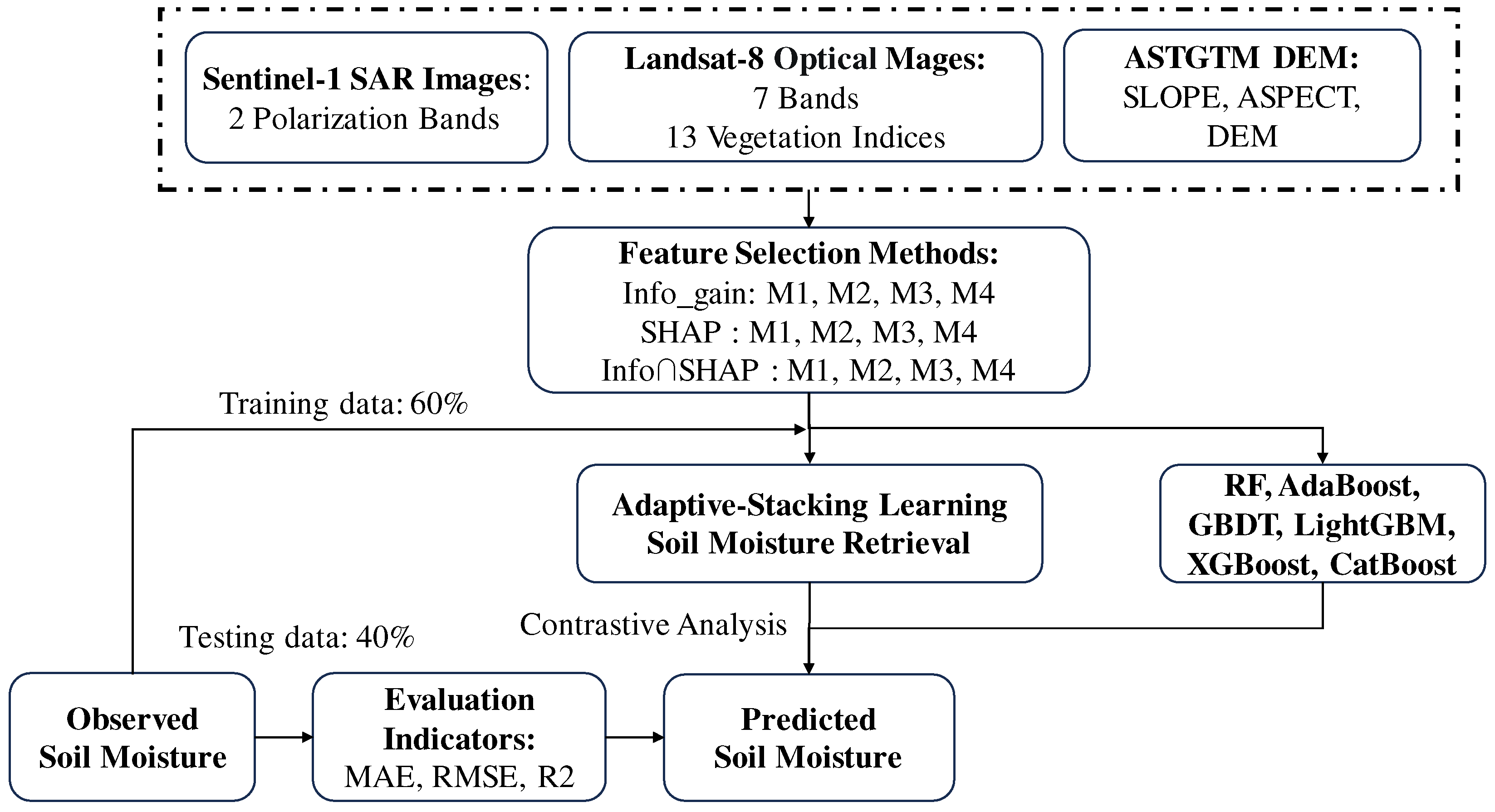
2.2. Dataset
2.2.1. Sentinel-1
2.2.2. Landsat-8
2.2.3. ASTGTM DEM
2.3. Method
2.3.1. Feature Selection Algorithm
2.3.2. Ada-Stacking Algorithm
- Initialize the weights of the training data.
- Utilize adaptive to iteratively train a set of weak classifiers. Each weak classifier is trained using the current sample weights.
- Predict the training data using the set of weak classifiers and obtain the prediction results for each sample.
- Aggregate the prediction results of the weak classifiers as new features and combine them with the original features.
- Apply the stacking method to train a meta-model using the combined features as input. An adaptive weight adjustment mechanism is proposed in this study to enhance the performance of the base learner. This mechanism dynamically adjusts the weights assigned to the base learner based on the comparison between the predicted outcomes and the actual labels. Weight adjustments are made by increasing the weights for base learners that exhibit smaller prediction errors and decreasing the weights for those with larger prediction errors.
- Utilize the trained meta-model to make predictions on the test data.
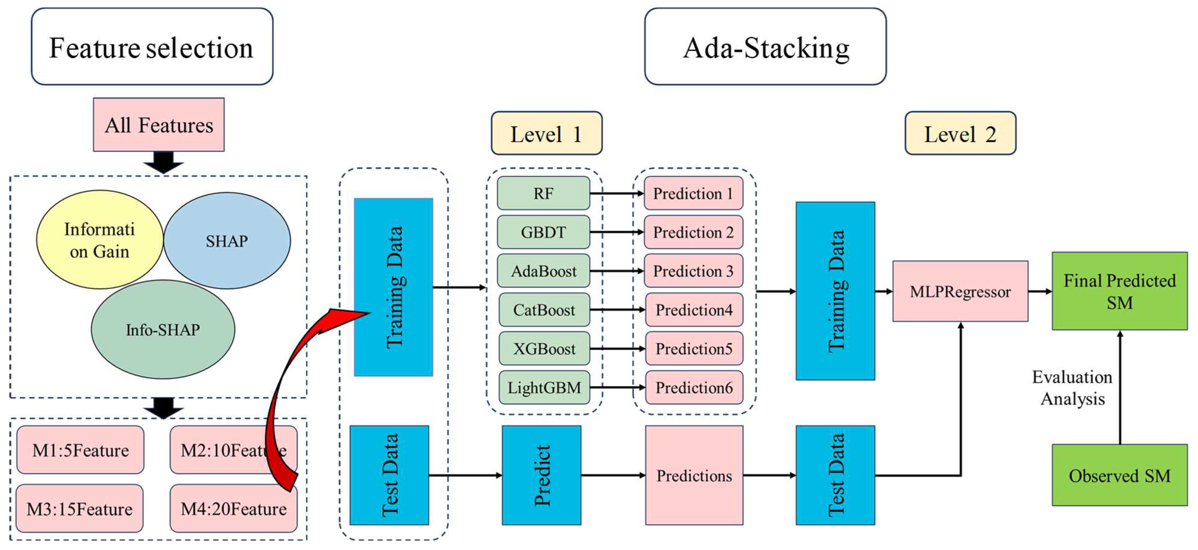
2.3.3. Overall Soil Moisture Retrieval Framework
- Dataset preparation: Partition the original dataset into a training set and a test set, ensuring dataset balance and representativeness.
- Initialization of training data weights: Initialize the weights of the training samples, either by evenly distributing them or adjusting them based on the sample categories.
- Iterative training of adaptive weak classifiers: Employ adaptive learning to train weak classifiers iteratively. In each round of training, a weak classifier is trained using the current sample weights. Typically, weaker-performing models are chosen as weak classifiers. The training of each weak classifier involves adjusting the sample weights based on the classification error rate from the previous round. This ensures that more attention is given to the misclassified samples in the subsequent rounds.
- Prediction using weak classifiers: Utilize the trained weak classifiers to predict both the training and test data.
- Construction of new features: Incorporate the prediction results of the weak classifiers as new features and combine them with the original features. These new features can be utilized in subsequent meta-model training.
- Meta-model training using the Ada-Stacking method: Employ the stacking method to train a meta-model, also known as a combined model, which takes the merged features as input for predicting the target variable. The first layer consists of six models: RF, AdaBoost, GBDT, LightGBM, XGBoost, and CatBoost. The second layer employs a multilayer perceptron for prediction. In our research, we have implemented an automated weight adjustment scheme within the stacking algorithm. This mechanism dynamically adjusts the weights assigned to each ML algorithm incorporated in the stacking ensemble. In the study of soil moisture inversion using ensemble learning algorithms, we employed a ten-fold cross-validation approach to evaluate the model performance. Specifically, we divided the entire dataset into training and validation sets. In total, 60% of the data were used as the training set to train the ensemble learning model, while the remaining 40% was allocated as the validation set to assess the model’s generalization ability and prediction accuracy.
- Meta-model prediction: Utilize the trained meta-model to predict the test data, obtaining the final predicted SM.
2.4. Model Evaluation Indicators
3. Results
3.1. Correlation Analysis of Feature Selection Results and Measured SM
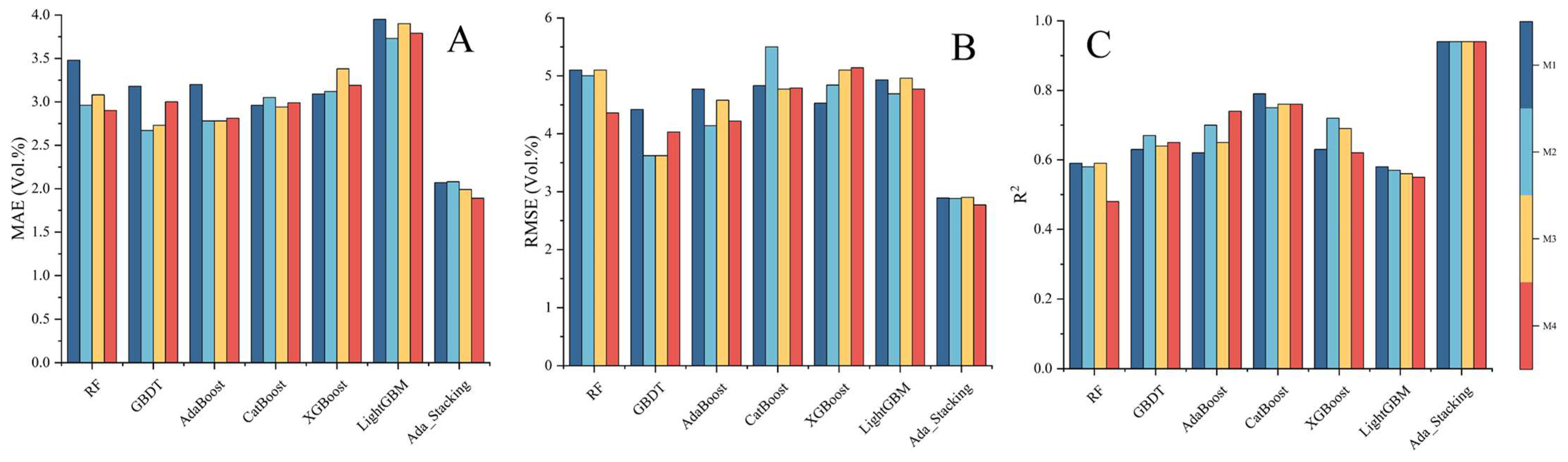
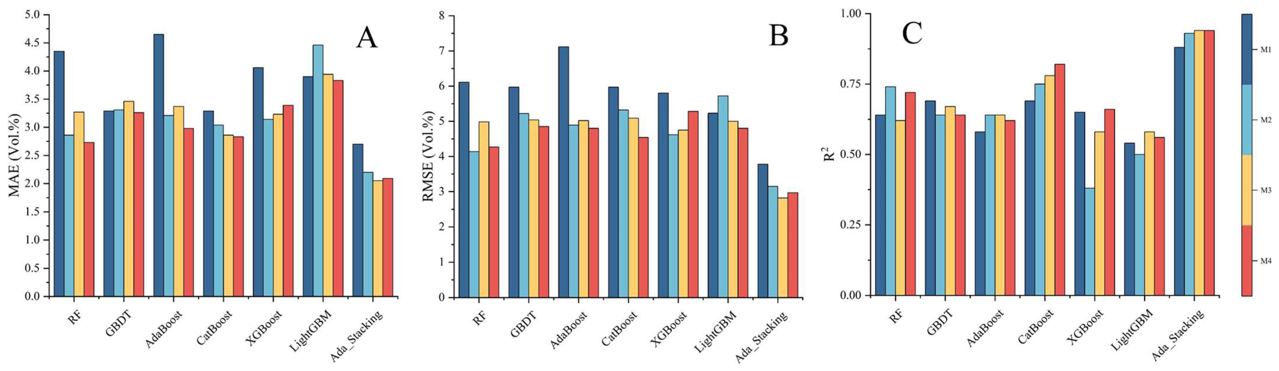
3.2. Evaluation and Comparison Under Different Feature Combinations and Different ML Methods
3.3. SM Inversion Results Based on Ada-Stacking Algorithm
4. Discussion
4.1. Comparison of Info_gain, SHAP and Info_gain ∩ SHAP for Variables Selection
4.2. Comparison of Ada-Stacking and Other ML Algorithms for SM Inversion
5. Conclusions
- Combining Info_gain and SHAP for feature selection effectively identifies the most informative and physically meaningful predictors by balancing statistical relevance (Info_gain) with model-specific nonlinear interactions (SHAP), thereby enhancing feature interpretability while reducing redundancy.
- The Ada-Stacking algorithm integrates adaptive boosting (AdaBoost) with stacked generalization, leveraging ensemble learning to mitigate overfitting and improve generalization across diverse vegetation and terrain conditions, where traditional single-model approaches often fail.
- This hybrid framework synergizes robust feature selection with advanced ensemble modeling, achieving higher accuracy in soil moisture retrieval—particularly in complex landscapes—by dynamically weighting base learners and optimizing meta-learner performance through iterative error correction.
Author Contributions
Funding
Data Availability Statement
Acknowledgments
Conflicts of Interest
References
- Babaeian, E.; Paheding, S.; Siddique, N.; Devabhaktuni, V.K.; Tuller, M. Estimation of root zone soil moisture from ground and remotely sensed soil information with multisensor data fusion and automated machine learning. Remote Sens. Environ. 2021, 260, 112434. [Google Scholar] [CrossRef]
- Peng, J.; Albergel, C.; Balenzano, A.; Brocca, L.; Cartus, O.; Cosh, M.H.; Crow, W.T.; Dabrowska-Zielinska, K.; Dadson, S.; Davidson, M.W.; et al. A roadmap for high-resolution satellite soil moisture applications-confronting product characteristics with user requirements. Remote Sens. Environ. 2020, 252, 112162. [Google Scholar] [CrossRef]
- Mayer, M.; Prescott, C.E.; Abaker, W.E.A.; Augusto, L.; Cécillon, L.; Ferreira, G.W.; James, J.; Jandl, R.; Katzensteiner, K.; Laclau, J.-P.; et al. Tamm Review: Influence of forest management activities on soil organic carbon stocks: A knowledge synthesis. Forest Ecol. Manag. 2020, 466, 118127. [Google Scholar] [CrossRef]
- Jamei, M.; Karbasi, M.; Malik, A.; Abualigah, L.; Islam, A.R.; Yaseen, Z.M. Computational assessment of groundwater salinity distribution within coastal multi-aquifers of Bangladesh. Sci. Rep. 2022, 12, 11165. [Google Scholar] [CrossRef]
- Senyurek, V.; Lei, F.; Boyd, D.; Gurbuz, A.C.; Kurum, M.; Moorhead, R. Evaluations of Machine Learning-Based CYGNSS Soil Moisture Estimates against SMAP Observations. Remote Sens.-Basel. 2020, 12, 3503. [Google Scholar] [CrossRef]
- Liu, L.; Gudmundsson, L.; Hauser, M.; Qin, D.; Li, S.; Seneviratne, S.I. Soil moisture dominates dryness stress on ecosystem production globally. Nat. Commun. 2020, 11, 4892. [Google Scholar] [CrossRef] [PubMed]
- Wang, L.; Gao, Y. Estimating and Downscaling ESA-CCI Soil Moisture Using Multi-Source Remote Sensing Images and Stacking-Based Ensemble Learning Algorithms in the Shandian River Basin, China. Remote Sens. 2025, 17, 716. [Google Scholar] [CrossRef]
- Lopes, C.L.; Mendes, R.; Caçador, I.; Dias, J.M. Assessing salt marsh loss and degradation by combining long-term Landsat imagery and numerical modelling. Land Degrad. Dev. 2021, 32, 4534–4545. [Google Scholar] [CrossRef]
- Tong, C.; Wang, H.; Magagi, R.; Goïta, K.; Zhu, L.; Yang, M.; Deng, J. Soil Moisture Retrievals by Combining Passive Microwave and Optical Data. Remote Sens. 2020, 12, 3173. [Google Scholar] [CrossRef]
- Delavar, M.A.; Naderi, A.; Ghorbani, Y.; Mehrpouyan, A.; Bakhshi, A. Soil salinity mapping by remote sensing south of Urmia Lake, Iran. Geoderma Reg. 2020, 22, e00317. [Google Scholar] [CrossRef]
- Muzalevskiy, K.; Zeyliger, A. Application of Sentinel-1B Polarimetric Observations to Soil Moisture Retrieval Using Neural Networks: Case Study for Bare Siberian Chernozem Soil. Remote Sens. 2021, 13, 3480. [Google Scholar] [CrossRef]
- Luo, M.; Wang, Y.; Xie, Y.; Zhou, L.; Qiao, J.; Qiu, S.; Sun, Y. Combination of Feature Selection and CatBoost for Prediction: The First Application to the Estimation of Aboveground Biomass. Forest 2021, 12, 216. [Google Scholar] [CrossRef]
- Al-Yaari, A.; Wigneron, J.P.; Dorigo, W.; Colliander, A.; Pellarin, T.; Hahn, S.; Mialon, A.; Richaume, P.; Fernandex-Moran, R.; Fan, L.; et al. Assessment and inter-comparison of recently developed/reprocessed microwave satellite soil moisture products using ISMN ground-based measurements. Remote Sens. Environ. 2019, 224, 289–303. [Google Scholar] [CrossRef]
- He, L.; Cheng, Y.; Li, Y.; Li, F.; Fan, K.; Li, Y. An Improved Method for Soil Moisture Monitoring With Ensemble Learning Methods Over the Tibetan Plateau. IEEE J. Sel. Top. Appl. Earth Obs. Remote Sens. 2021, 14, 2833–2844. [Google Scholar] [CrossRef]
- Lary, D.J.; Remer, L.A.; MacNeill, D.; Roscoe, B.; Paradise, S. Machine Learning and Bias Correction of MODIS Aerosol Optical Depth. IEEE Geosci. Remote Sens. Lett. 2009, 6, 694–698. [Google Scholar] [CrossRef]
- Ma, L.; Liu, Y.; Zhang, X.; Ye, Y.; Yin, G.; Johnson, B.A. Deep learning in remote sensing applications: A meta-analysis and review. ISPRS J. Photogramm. Remote Sens. 2019, 152, 166–177. [Google Scholar] [CrossRef]
- Zhang, Y.; Liu, J.; Shen, W. Review of Ensemble Learning Algorithms Used in Remote Sensing Applications. Appl. Sci. 2022, 12, 8654. [Google Scholar] [CrossRef]
- Jamei, M.; Ali, M.; Karbasi, M.; Sharma, E.; Jamei, M.; Chu, X.; Yaseen, Z.M. A high dimensional features-based cascaded forward neural network coupled with MVMD and Boruta-GBDT for multi-step ahead forecasting of surface soil moisture. Eng. Appl. Artif. Intel. 2023, 120, 105895. [Google Scholar] [CrossRef]
- Nguyen, T.T.; Ngo, H.H.; Guo, W.; Chang, S.W.; Nguyen, D.D.; Nguyen, C.T.; Zhang, J.; Liang, S.; Bui, X.T.; Hoang, N.B. A low-cost approach for soil moisture prediction using multi-sensor data and machine learning algorithm. Sci. Total Environ. 2022, 833, 155066. [Google Scholar] [CrossRef]
- Chen, L.; Xing, M.; He, B.; Wang, J.; Shang, J.; Huang, X.; Xu, M. Estimating Soil Moisture Over Winter Wheat Fields During Growing Season Using Machine-Learning Methods. IEEE J. Sel. Top. Appl. Earth Obs. Remote Sens. 2021, 14, 3706–3718. [Google Scholar] [CrossRef]
- Zhang, L.; Zhang, Z.; Xue, Z.; Li, H. Sensitive Feature Evaluation for Soil Moisture Retrieval Based on Multi-Source Remote Sensing Data with Few In-Situ Measurements: A Case Study of the Continental, U.S. Water 2021, 13, 2003. [Google Scholar] [CrossRef]
- Gao, Y.; Wang, L.; Zhong, G.; Wang, Y.; Yang, J. Potential of Remote Sensing Images for Soil Moisture Retrieving Using Ensemble Learning Methods in Vegetation-Covered Area. IEEE J.-STARS 2023, 16, 8149–8165. [Google Scholar] [CrossRef]
- Wang, S.; Wu, Y.; Li, R.; Wang, X. Remote sensing-based retrieval of soil moisture content using stacking ensemble learning models. Land Degrad. 2023, 34, 911–925. [Google Scholar] [CrossRef]
- Zhao, T.; Shi, J.; Lv, L.; Xu, H.; Chen, D.; Cui, Q.; Jackson, T.J.; Yan, G.; Jia, L.; Chen, L.; et al. Soil moisture experiment in the Luan River supporting new satellite mission opportunities. Remote Sens. Environ. 2020, 240, 111680. [Google Scholar] [CrossRef]
- Zhao, T.; Yao, P.; Cui, Q.; Jiang, L.; Chai, L.; Lu, H.; Ma, J.; Lv, H.; Wu, J.; Zhao, W.; et al. Synchronous Observation Data Set of Soil Temperature and Soil Moisture in the Upstream of Luan River (2018); National Tibetan Plateau, Ed.; National Tibetan Plateau Data Center: Beijing, China, 2021. [Google Scholar]
- Amazirh, A.; Merlin, O.; Er-Raki, S.; Gao, Q.; Rivalland, V.; Malbeteau, Y.; Khabba, S.; Escorihuela, M.J. Retrieving surface soil moisture at high spatio-temporal resolution from a synergy between Sentinel-1 radar and Landsat thermal data: A study case over bare soil. Remote Sens. Environ. 2018, 211, 321–337. [Google Scholar] [CrossRef]
- Chaudhary, S.K.; Srivastava, P.K.; Gupta, D.K.; Kumar, P.; Prasad, R.; Pandey, D.K.; Das, A.K.; Gupta, M. Machine learning algorithms for soil moisture estimation using Sentinel-1: Model development and implementation. Adv. Space Res. 2022, 69, 1799–1812. [Google Scholar] [CrossRef]
- Zhang, Y.; Liang, S.; Zhu, Z.; Ma, H.; He, T. Soil moisture content retrieval from Landsat 8 data using ensemble learning. ISPRS J. Photogramm. Remote Sens. 2022, 185, 32–47. [Google Scholar] [CrossRef]
- Ghasemloo, N.; Matkan, A.A.; Alimohammadi, A.; Aghighi, H.; Mirbagheri, B. Estimating the Agricultural Farm Soil Moisture Using Spectral Indices of Landsat 8, and Sentinel-1, and Artificial Neural Networks. J. Geovisualization Spat. Analysis 2022, 6, 19. [Google Scholar] [CrossRef]
- Filippucci, P.; Brocca, L.; Quast, R.; Ciabatta, L.; Saltalippi, C.; Wagner, W.; Tarpanelli, A. High-resolution (1 km) satellite rainfall estimation from SM2RAIN applied to Sentinel-1: Po River basin as a case study. Hydrol. Earth Syst. Sci. 2022, 26, 2481–2497. [Google Scholar] [CrossRef]
- Khandelwal, S.; Goyal, R.; Kaul, N.; Mathew, A. Assessment of land surface temperature variation due to change in elevation of area surrounding Jaipur, India. Egypt. J. Remote Sens. Space Sci. 2017, 21, 87–94. [Google Scholar] [CrossRef]
- Naji, T.A. Study of vegetation cover distribution using DVI, PVI, WDVI indices with 2D-space plot. J. Phys. Conf. Ser. 2018, 1003, 012083. [Google Scholar] [CrossRef]
- Gurung, R.B.; Breidt, F.J.; Dutin, A.; Ogle, S.M. Predicting Enhanced Vegetation Index (EVI) curves for ecosystem modeling applications. Remote Sens. Environ. 2009, 113, 2186–2193. [Google Scholar] [CrossRef]
- Zhang, Y.; Tan, K.; Wang, X.; Chen, Y. Retrieval of soil moisture content based on a modified Hapke Photometric model: A novel method applied to laboratory hyperspectral and Sentinel-2 MSI data. Remote Sens. 2020, 12, 2239. [Google Scholar] [CrossRef]
- Wu, C.; Niu, Z.; Tang, Q.; Huang, W. Estimating chlorophyll content from hyperspectral vegetation indices: Modeling and validation. Agric. For. Meteorol. 2008, 148, 1230–1241. [Google Scholar] [CrossRef]
- Pettorelli, N.; Ryan, S.; Mueller, T.; Bunnefeld, N.; Jędrzejewska, B.; Lima, M.; Kausrud, K. The Normalized Difference Vegetation Index (NDVI): Unforeseen successes in animal ecology. Clim. Res. 2011, 46, 15–27. [Google Scholar] [CrossRef]
- Huang, J.; Chen, D.; Cosh, M.H. Sub-pixel reflectance unmixing in estimating vegetation water content and dry biomass of corn and soybeans cropland using normalized difference water index (NDWI) from satellites. Int. J. Remote Sens. 2009, 30, 2075–2104. [Google Scholar] [CrossRef]
- Meng, Q.; Xie, Q.; Wang, C.; Ma, J.; Sun, Y.; Zhang, L. A fusion approach of the improved Dubois model and best canopy water retrieval models to retrieve soil moisture through all maize growth stages from Radarsat-2 and Landsat-8 data. Environ. Earth Sci. 2016, 75, 1377. [Google Scholar] [CrossRef]
- Wang, L.; Qu, J.J. NMDI: A normalized multi-band drought index for monitoring soil and vegetation moisture with satellite remote sensing. Geophys. Res. Lett. 2007, 34, L20405. [Google Scholar] [CrossRef]
- Major, D.J.; Baret, F.; Guyot, G. A ratio vegetation index adjusted for soil brightness. Int. J. Remote Sens. 1990, 11, 727–740. [Google Scholar] [CrossRef]
- Huete, A.R. A soil-adjusted vegetation index (SAVI). Remote Sens. Environ. 1988, 25, 295–309. [Google Scholar] [CrossRef]
- Payero, J.O.; Neale, C.M.; Wright, J.L. Comparison of eleven vegetation indices for estimating plant height of alfalfa and grass. Appl. Eng. Agric. 2004, 20, 385–393. [Google Scholar] [CrossRef]
- Kaufman, Y.J.; Tanre, D. Atmospherically resistant vegetation index (ARVI) for EOS-MODIS, IEEE T. Geosci. Remote 1992, 30, 261–270. [Google Scholar] [CrossRef]
- Robinove, C.J.; Chavez, P.S., Jr.; Gehring, D.; Holmgren, R. Arid land monitoring using Landsat albedo difference images. Remote Sens. Environ. 1981, 11, 133–156. [Google Scholar] [CrossRef]
- Bugaj, M.; Wrobel, K.; Iwaniec, J. Model explainability using SHAP values for LightGBM predictions. In Proceedings of the 2021 IEEE XVIIth International Conference on the Perspective Technologies and Methods in MEMS Design (MEMSTECH), Polyana, Ukraine, 12 May 2021; pp. 102–106. [Google Scholar]
- Marcilio, W.E.; Eler, D.M. From explanations to feature selection: Assessing SHAP values as feature selection mechanism. In Proceedings of the 33rd SIBGRAPI Conference on Graphics, Patterns and Images (SIBGRAPI), Porto de Galinhas, Brazil, 7–10 November 2020; pp. 340–347. [Google Scholar]
- Prasetyo, S.E.; Prastyo, P.H.; Arti, S. A cardiotocographic classification using feature selection: A comparative study. JITCE J. Inf. Technol. Comput. Eng. 2021, 5, 25–32. [Google Scholar] [CrossRef]
- Dey, S.K.; Raihan Uddin, M.; Mahbubur Rahman, M. Performance analysis of SDN-based intrusion detection model with feature selection approach. In Proceedings of the International Joint Conference on Computational Intelligence: IJCCI 2018, Seville, Spain, 18–19 September 2020; pp. 483–494. [Google Scholar]
- Uğuz, H. A two-stage feature selection method for text categorization by using information gain, principal component analysis and genetic algorithm. Knowl.-Based Syst. 2011, 24, 1024–1032. [Google Scholar] [CrossRef]
- Pereira, R.B.; Plastino, A.; Zadrozny, B.; Merschmann, L.H. Information gain feature selection for multi-label classification. J. Inf. Data Manag. 2015, 6, 48. [Google Scholar]
- Prasetiyowati, M.I.; Maulidevi, N.U.; Surendro, K. Determining threshold value on information gain feature selection to increase speed and prediction accuracy of random forest. J. Big Data 2021, 8, 84. [Google Scholar] [CrossRef]
- Gao, Z.; Xu, Y.; Meng, F.; Qi, F.; Lin, Z. Improved information gain-based feature selection for text categorization. In Proceedings of the 2014 4th International Conference on Wireless Communications, Vehicular Technology, Information Theory and Aerospace & Electronic Systems (VITAE), Aalborg, Denmark, 11–14 May 2014; pp. 1–5. [Google Scholar] [CrossRef]
- Yi, F.; Yang, H.; Chen, D.; Qin., Y.; Han, H.; Cui, J.; Bai, W.; Ma, Y.; Zhang, R.; Yu, H. XGBoost-SHAP-based interpretable diagnostic framework for alzheimer’s disease. BMC Med. Inform. Decis. 2023, 23, 137. [Google Scholar] [CrossRef] [PubMed]
- Mora, T.; Roche, D.; Rodríguez-Sánchez, B. Predicting the onset of diabetes-related complications after a diabetes diagnosis with machine learning algorithms. Diabetes Res. Clin. Pract. 2023, 204, 110910. [Google Scholar] [CrossRef] [PubMed]
- Pavon, J.M.; Previll, L.; Woo, M.; Henao, R.; Solomon, M.; Rogers, U.; Olson, A.; Fischer, J.; Leo, C.; Fillenbaum, G.; et al. Machine learning functional impairment classification with electronic health record data. J. Am. Geriatr. Soc. 2023, 71, 2822–2833. [Google Scholar] [CrossRef]
- Kim, J.; Lee, H.; Lee, J.; Rhee, S.Y.; Shin, J.I.; Lee, S.W.; Cho, W.; Min, C.; Kwon, R.; Kim, J.G.; et al. Quantification of identifying cognitive impairment using olfactory-stimulated functional near-infrared spectroscopy with machine learning: A post hoc analysis of a diagnostic trial and validation of an external additional trial. Alzheimer’s Res. Ther. 2023, 15, 127. [Google Scholar] [CrossRef] [PubMed]
- Ye, Z.; Zhang, T.; Wu, C.; Qiao, Y.; Su, W.; Chen, J.; Xie, G.; Dong, S.; Xu, J.; Zhao, J. Predicting the objective and subjective clinical outcomes of anterior cruciate ligament reconstruction: A machine learning analysis of 432 patients. Am. J. Sports Med. 2022, 50, 3786–3795. [Google Scholar] [CrossRef]
- Das, B.; Rathore, P.; Roy, D.; Chakraborty, D.; Jatav, R.S.; Sethi, D.; Kumar, P. Comparison of bagging, boosting and stacking algorithms for surface soil moisture mapping using optical-thermal-microwave remote sensing synergies. Catena 2022, 217, 106485. [Google Scholar] [CrossRef]
- Tao, S.; Zhang, X.; Feng, R.; Qi, W.; Wang, Y.; Shrestha, B. Retrieving soil moisture from grape growing areas using multi-feature and stacking-based ensemble learning modeling. Comput. Electron. Agric. 2023, 204, 107537. [Google Scholar] [CrossRef]
- Granata, F.; Di Nunno, F.; Najafzadeh, M.; Demir, I. A stacked machine learning algorithm for multi-step ahead prediction of soil moisture. Hydrology 2022, 10, 1. [Google Scholar] [CrossRef]
- Paramythis, A.; Loidl-Reisinger, S. Adaptive learning environments and e-learning standards. In Proceedings of the 2nd European Conference on E-Learning, Linz, Austria, 6–7 November 2003; pp. 369–379. [Google Scholar]
- Kerr, P. Adaptive learning. Elt J. 2016, 70, 88–93. [Google Scholar] [CrossRef]
- Zeiler, M.D. Adadelta: An adaptive learning rate method. arXiv 2012, arXiv:1212.5701. [Google Scholar]
- Frías-Blanco, I.; Verdecia-Cabrera, A.; Ortiz-Díaz, A.; Carvalho, A. Fast adaptive stacking of ensembles. In Proceedings of the 31st Annual ACM Symposium on Applied Computing, Pisa, Italy, 4 April 2016; pp. 929–934. [Google Scholar]
- Agarwal, S.; Chowdary, C.R. A-Stacking and A-Bagging: Adaptive versions of ensemble learning algorithms for spoof fingerprint detection. Expert Syst. 2020, 146, 113160. [Google Scholar] [CrossRef]


| Satellite Name | Parameters | Description |
|---|---|---|
| Sentinel-1 | VV | Backscattering coefficient |
| VH | ||
| Landsat-8 | B1 | Coastal |
| B2 | Blue | |
| B3 | Green | |
| B4 | Red | |
| B5 | NIR | |
| B6 | SWIR-1 | |
| B7 | SWIR-2 | |
| Multi-vegetation index | See Table 2 for details | |
| ASTGTM DEM | Slope | Maximum rate of change in elevation |
| Aspect | Direction of projection of the slope; normal on the horizontal plane | |
| DEM | Digital Elevation Model |
| Parameters | Description | References |
|---|---|---|
| Difference Vegetation Index (DVI) | DVI = b5 − b4 | [32] |
| Enhanced Vegetation Index (EVI) | EVI = 2.5 × (b5 − b4)/(b5 + 6 × b4 − 7.5 × b2 + 1) | [33] |
| Modified Soil Index (MSI) | MSI = b6/b5 | [34] |
| Modified Senescent Reflectance Index (MSR) | MSR = (b5/b4 − 1)/Sqrt(b5/b4 + 1) | [35] |
| Normalized Difference Vegetation Index (NDVI) | NDVI = (b5 − b4)/(b5 + b4) | [36] |
| Normalized Difference Water Index (NDWI1640) | NDWI1640 = (b5 − b6)/(b5 + b6) | [37] |
| Normalized Difference Water Index (NDWI2201) | NDWI2201 = (b5 − b7)/(b5 + b7) | [38] |
| Normalized Multi-Band Drought Index (NMDI) | NMDI = (b5 − (b6 − b5))/(b5 + (b6 + b5)) | [39] |
| Ratio Vegetation Index (RVI) | RVI = b5/b4 | [40] |
| Soil-Adjusted Vegetation Index (SAVI) | SAVI = (b5 − b4) × (1 + 0.5)/(b5 + b4 + 0.5) | [41] |
| Transformed Vegetation Index (TVI) | TVI = 0.5 × (120 × (b5 − b3) – 200 × (b4 − b3)) | [42] |
| Atmospherically Resistant Vegetation Index (ARVI) | ARVI = (b5 − (2 × b4 − b2))/(b5 + (2 × b4 − b2)) | [43] |
| Albedo (reflectance) index (Albedo) | Albedo = 0.356 × b2 + 0.13 × b3 + 0.373 × b4 + 0.085 × b5 + 0.072 × b6 + 0.072 × b7 − 0.0018 | [44] |
| Feature Selection Method and Number of Features | Specific Characteristics |
|---|---|
| Info_gain_M1 | DEM, DVI, MSI, VV, NMDI |
| Info_gain_M2 | DEM, DVI, MSI, VV, NMDI, NDWI1640, EVI, VH, B5, TVI |
| Info_gain_M3 | DEM, DVI, MSI, VV, NMDI, NDWI1640, EVI, VH, B5, TVI, NDWI2201, B6, RVI, B1, SAVI |
| Info_gain_M4 | DEM, DVI, MSI, VV, NMDI, NDWI1640, EVI, VH, B5, TVI, NDWI2201, B6, RVI, B1, SAVI, Albedo, ARVI, NDVI, B3, aspect |
| SHAP_M1 | DEM, VV, slope, B1, EVI |
| SHAP_M2 | DEM, VV, slope, B1, EVI, VH, ARVI, B6, TVI, DVI |
| SHAP_M3 | DEM, VV, slope, B1, EVI, VH, ARVI, B6, TVI, DVI, B4, aspect, B2, B3, MSI |
| SHAP_M4 | DEM, VV, slope, B1, EVI, VH, ARVI, B6, TVI, DVI, B4, aspect, B2, B3, MSI, B5, NDWI2201, NDWI1640, Albedo, SAVI |
| Info_gain ∩ SHAP_M1 | DEM, VV |
| Info_gain ∩ SHAP_M2 | DEM, VV, DVI, EVI, VH, TVI |
| Info_gain ∩ SHAP_M3 | DEM, VV, DVI, EVI, VH, TVI, B1 |
| Info_gain ∩ SHAP_M4 | DEM, VV, DVI, EVI, VH, TVI, B1, ARVI, aspect, B3, MSI, B5, NDWI2201, NDWI1640, Albedo, SAVI |
| MAE (Vol. %) | RMSE (Vol.%) | R2 | |
|---|---|---|---|
| Ada_Stacking_Info_gain_M1 | 2.23 | 3.06 | 0.94 |
| Ada_Stacking_Info_gain_M2 | 2.06 | 2.77 | 0.94 |
| Ada_Stacking_Info_gain_M3 | 2.08 | 2.89 | 0.94 |
| Ada_Stacking_Info_gain_M4 | 1.86 | 2.68 | 0.95 |
| Ada_Stacking_SHAP_M1 | 2.07 | 2.89 | 0.94 |
| Ada_Stacking_SHAP_M2 | 2.08 | 2.88 | 0.94 |
| Ada_Stacking_SHAP_M3 | 1.99 | 2.9 | 0.94 |
| Ada_Stacking_SHAP_M4 | 1.89 | 2.77 | 0.94 |
| Ada_Stacking_Info_gain ∩SHAP_M1 | 2.7 | 3.78 | 0.88 |
| Ada_Stacking_Info_gain ∩ SHAP_M2 | 2.2 | 3.15 | 0.93 |
| Ada_Stacking_Info_gain ∩ SHAP_M3 | 2.05 | 2.82 | 0.94 |
| Ada_Stacking_Info_gain ∩ SHAP_M4 | 2.09 | 2.97 | 0.94 |
Disclaimer/Publisher’s Note: The statements, opinions and data contained in all publications are solely those of the individual author(s) and contributor(s) and not of MDPI and/or the editor(s). MDPI and/or the editor(s) disclaim responsibility for any injury to people or property resulting from any ideas, methods, instructions or products referred to in the content. |
© 2025 by the authors. Licensee MDPI, Basel, Switzerland. This article is an open access article distributed under the terms and conditions of the Creative Commons Attribution (CC BY) license (https://creativecommons.org/licenses/by/4.0/).
Share and Cite
Wang, L.; Gao, Y. Soil Moisture Inversion Using Multi-Sensor Remote Sensing Data Based on Feature Selection Method and Adaptive Stacking Algorithm. Remote Sens. 2025, 17, 1569. https://doi.org/10.3390/rs17091569
Wang L, Gao Y. Soil Moisture Inversion Using Multi-Sensor Remote Sensing Data Based on Feature Selection Method and Adaptive Stacking Algorithm. Remote Sensing. 2025; 17(9):1569. https://doi.org/10.3390/rs17091569
Chicago/Turabian StyleWang, Liguo, and Ya Gao. 2025. "Soil Moisture Inversion Using Multi-Sensor Remote Sensing Data Based on Feature Selection Method and Adaptive Stacking Algorithm" Remote Sensing 17, no. 9: 1569. https://doi.org/10.3390/rs17091569
APA StyleWang, L., & Gao, Y. (2025). Soil Moisture Inversion Using Multi-Sensor Remote Sensing Data Based on Feature Selection Method and Adaptive Stacking Algorithm. Remote Sensing, 17(9), 1569. https://doi.org/10.3390/rs17091569