Real-Time Regional Ionospheric Total Electron Content Modeling Using the Extended Kalman Filter

Abstract

Real-time ionospheric products can accelerate the convergence of real-time precise point positioning (PPP) to improve the real-time positioning services of global navigation satellite systems (GNSSs), as well as to achieve continuous monitoring of the ionosphere. This study applied an extended Kalman filter (EKF) to total electron content (TEC) modeling, proposing a regional real-time EKF-based ionospheric model (REIM) with a spatial resolution of 1° × 1° and a temporal resolution of 1 h. We examined the performance of REIM through a 7-day period during geomagnetic storms. The post-processing model from the China Earthquake Administration (IOSR), CODG, IGSG, and the BDS geostationary orbit satellite (GEO) observations were utilized as reference. The consistency analysis showed that the mean deviation between REIM and IOSR was 0.97 TECU, with correlation coefficients of 0.936 and 0.938 relative to IOSR and IGSG, respectively. The VTEC mean deviation between REIM and BDS GEO observations was 4.15 TECU, which is lower than those of CODG (4.68 TECU), IGSG (5.67 TECU), and IOSR (6.27 TECU). In the real-time single-frequency PPP (RT-SF-PPP) experiments, REIM-augmented positioning converges within approximately 80 epochs, and IGSG requires 140 epochs. The REIM-augmented east-direction positioning error was 0.086 m, smaller than that of IGSG (0.095 m) and the Klobuchar model (0.098 m). REIM demonstrated high consistencies with post-processing models and showed a higher accuracy at IPPs of BDS GEO satellites. Moreover, the correction results of the REIM model are comparable to post-processing models in RT-SF-PPP while achieving faster convergence.

1. Introduction

The ionosphere refers to the atmosphere between 60 and 1000 km above the Earth’s surface. Because of the large number of free electrons, it is one of the most significant error sources affecting the positioning precision of the global navigation satellite system (GNSS) [1]. Ionosphere delay increases GNSS measurement errors, limiting the ability of GNSS to achieve real-time high-precision positioning [2]. Modeling ionospheric total electron content (TEC) to correct the ionospheric delay is an effective way to increase accuracy and convergence speed in precise point positioning (PPP), enabling high-precision real-time positioning.

In 1998, the International GNSS Service (IGS) was founded, and IGS Ionosphere Associate Analysis Centers (IAACs) were established as the primary center for GNSS data processing and analysis. Today, global GNSS ionospheric analysis centers have been developed worldwide, including the Center of Orbit Determination in Europe (CODE), the Jet Propulsion Laboratory (JPL), the Universitat Politècnica de Catalunya (UPC), the European Space Agency (ESA), the Chinese Academy of Sciences (CAS), and Wuhan University (WHU) [3]. These analysis centers adopt different strategies to generate a variety of GIM products [4,5], providing a large amount of high-precision data for ionospheric monitoring. Users can derive regional ionospheric maps by interpolating the GIMs, which are available in ionosphere map exchange format (IONEX) [6]. However, post-processing ionosphere models from analysis centers exhibit a delay of 1–2 days [7], rendering them incapable of high-precision real-time ionosphere monitoring and ionosphere delay corrections. Thus, IAAC has been actively developing real-time ionosphere TEC models, and some preliminary progress has been achieved. For example, the GIM forecast products show potential for real-time and near-real-time ionospheric delay correction [8]. Currently, real-time GIM products show significantly lower precision compared to post-processing GIMs, requiring further improvements to meet the demands of various practical applications [9].

In recent years, regional ionospheric modeling has developed rapidly in China. The two-layer spherical harmonics (SH) approximation method has been applied to real-time ionospheric modeling over China, showing better performance compared to the single-layer model in kinematic SF-PPP [1]. A new post-processing ionospheric model for the region over China has been established using GNSS observations from the Crustal Movement Observation Network of China (CMONOC), with a correlation analysis conducted against the IGS GIM [10]. These studies highlight the improvement in real-time ionospheric modeling in China; however, there remains a lack of experimental analysis regarding model performance during geomagnetic storms. Furthermore, more studies are needed to assess the application of the ionospheric model for positioning in China.

A common approach for real-time ionospheric TEC modeling is to combine the least squares method with the sliding window technique for parameter estimation. La Plata National University employs multi-frequency and multi-system GNSS observations in conjunction with sliding windows and weighted least squares to build real-time ionosphere models over the South American region. The models achieve a temporal resolution of 15 min and a spatial resolution of 0.5° × 0.5° [11,12]. It should be noted that the real-time data streams provided by IGS monitoring stations are limited to approximately 180 stations, which constrains the available ionospheric observations during specific periods. The uneven distribution of GNSS stations also results in decreased precision of parameter estimation in some regions when using methods like least squares or sliding window techniques. Additionally, building real-time ionospheric models for short-term forecasting requires substantial real-time data from globally distributed continuously operating reference station (CORS) and low Earth orbit (LEO) satellites, including the Swarm constellation and the Gravity Recovery and Climate Experiment (GRACE) satellites. The sliding window approach involves repeated use of data within the window to construct the normal equations, leading to data redundancy and affecting the efficiency of parameter estimation. The Kalman filter (KF) is effective in addressing the data redundancy problem. Once the initial state of the system is determined, the subsequent state can be estimated using the system’s state equations, the state estimates of the previous epoch, and current observations [13] without storing a large volume of historical data. As early as 1996, the National Oceanic and Atmospheric Administration (NOAA) used ground-based GNSS data from the CORS network in the United States to develop real-time TEC models using tomography and Kalman filtering methods [11]. More recently, researchers have integrated B-splines with Kalman filtering for rapid vertical TEC (VTEC) estimation, generating near real-time products with a delay of 2.5 h [14]. However, observation noise in real measuring systems is usually nonlinear, while KF is based on linear assumptions. Hence, linearization is necessary for its application.

Empirical broadcast ionosphere models, such as the international reference ionosphere (IRI) model [15] and the Klobuchar model proposed by the National Aeronautics Space Administration (NASA) [16], are also commonly applied in the current real-time navigation. Chen et al. [17] adopted the nonlinear least squares method to fit undetermined coefficients and proposed a multi-parameter fusion empirical model for forecasting ionospheric TEC over China. However, the precision of ionospheric delay corrections using these empirical models remains limited; for example, the percentage of ionospheric delay correction for the Beidou navigation satellite system (BDS) using the Klobuchar model is less than 60% [16,17]. Moreover, previous studies mainly focus on the differences between the compared models in China’s region, often lacking a stable and static reference to assess various models [18]. With the development of machine learning and deep learning, some researchers have begun exploring an integration of these techniques with ionospheric TEC forecasting and nowcasting. Srivani et al. [19] applied long short-term memory (LSTM) to train long-term datasets for ionosphere TEC forecasting and achieved an accuracy of 2 TEC Unit (TECU) during geomagnetically active periods. A generative adversarial networks model based on Poisson blending was utilized to train GIMs; the result shows better forecasting performance than conventional models during various solar activity periods [20]. Ruwali et al. [21] developed a combined model based on recurrent neural networks (RNN), which demonstrates higher correlations in TEC forecasting compared with single models. Nevertheless, these deep learning-based models are generally limited to single-station or small regions, and the accuracy and selection of datasets require further improvement and careful consideration.

This study aimed to build a real-time ionosphere TEC model using large-scale GNSS multi-system observations from ground-based reference stations in China. Data integration plays a crucial role in the real-time TEC modeling process. The ionosphere modeling coefficients and differential code bias (DCB) of subsequent epochs were estimated by incorporating the extended Kalman filter (EKF) algorithm, thereby forming the real-time EKF-based ionospheric model (REIM). By focusing on geomagnetic storm periods, we evaluated the performance of the REIM model through consistency analysis with post-processing models and comparison with static VTECs calculated at the ionospheric pierce points (IPPs) of BDS geostationary Earth orbit (GEO) satellites. Finally, the model was applied in real-time single-frequency precise point positioning (RT-SF-PPP), and the result shows it can reduce PPP convergence time. Therefore, the REMIME model is valuable for both positioning and navigation, as well as high-precision real-time ionosphere monitoring.

2. Methodology

Observation noise is typically nonlinear in real-world measuring. This study employed the EKF to estimate the parameters of the ionospheric model. The EKF can linearize nonlinear noise in real time, enabling the subsequent use of the Kalman filter for parameter forecasting and estimation. This method effectively addresses the issue of data redundancy.

2.1. Kalman Filtering Algorithm

The KF is a state estimation algorithm that was proposed in the early 1960s. Its advantage lies in the ability to handle linear systems and perform recursive state estimation without requiring the storage of a large amount of historical observational data. The state and measurement equations at time k can be represented as follows:

$$\left\{\begin{array}{l}{x}_k=A_k{x}_{k-1}+B_k{u}_{k-1}+w_{k-1}\hfill \\ y_k=C_k{x}_k+v_k\hfill \end{array}\right.,$$

(1)

where $x_k$ is the state vector at time k, $u_k$ is the input at time k, $A_k$ is the state-transition matrix, $B_k$ is the input-control matrix, $C_k$ is the observation matrix, and $w_k$ and $v_k$ are the process noise and measurement noise at time k, respectively [13]. $w_k$ and $v_k$ are zero-mean and uncorrelated Gaussian white noises as follows:

$$\left\{\begin{array}{l}E\left[w_k\right]=0,E\left[v_k\right]=0\hfill \\ \mathrm{cov}\left[w_k,w_j\right]=E\left[w_k{w}_j^T\right]=Q_k{\delta }_{kj}\hfill \\ \mathrm{cov}\left[v_k,v_j\right]=E\left[v_k{v}_j^T\right]=R_k{\delta }_{kj}\hfill \\ \mathrm{cov}\left[w_k,v_j\right]=E\left[w_k{v}_j^T\right]=0\hfill \end{array}\right.,$$

(2)

where $Q_k$ is the system noise matrix, $R_k$ is the measurement noise matrix, and ${\delta }_{kj}$ is the Kronecker function. The KF process includes two phases: state update and measurement update, with detailed explanations available in Erdogan et al. [14].

2.2. Extended Kalman Filtering Algorithm

The ionosphere is generally dynamic and nonlinear, while the EKF is capable of handling such nonlinear systems [22]. With the linearization equation in the EKF, the nonlinear modeling can be transformed into a linear one, achieving effective estimation and forecasting of the ionospheric state. The principle of EKF is to approximate the nonlinear function for linearization using only the first-order term in the Taylor series expansion while ignoring the second- and higher-order terms. This approach can improve the accuracy and stability of the filter when dealing with nonlinear systems. The state-space equations for a nonlinear system are as follows:

$$\left\{\begin{array}{l}{x}_k=f\left(x_{k-1},u_{k-1}\right)+w_{k-1}\hfill \\ y_k=h\left(x_k,u_k\right)+v_k\hfill \end{array}\right.,$$

(3)

where f () represents the nonlinear state function of the system, and h () represents the measurement function. In Equation (3), the nonlinear function f () is expanded at the estimated value ${\widehat{x}}_{k-1}$ using Taylor expansion, and similarly, h () is expanded at the predicted value of the current iteration $x_k$, retaining only the first-order terms, as shown in Equation (4). Substituting Equation (3) into Equation (4) forms Equation (5):

$$\left\{\begin{array}{l}f\left(x_{k-1},u_{k-1}\right)=f\left({\widehat{x}}_{k-1},u_{k-1}\right)+{\left.{\displaystyle \frac{\partial f\left(x_{k-1},u_{k-1}\right)}{\partial x_{k-1}}}\right|}_{x_{k-1}={\widehat{x}}_{k-1}}\left(x_{k-1}-{\widehat{x}}_{k-1}\right)\hfill \\ h\left(x_k,u_k\right)=h\left({\widehat{x}}_k,u_k\right)+{\left.{\displaystyle \frac{\partial h\left(x_k,u_k\right)}{\partial x_k}}\right|}_{x_{k-1}={\widehat{x}}_{k-1}}\left(x_{k-1}-{\widehat{x}}_{k-1}\right)\hfill \end{array}\right.,$$

(4)

$$\left\{\begin{array}{l}{x}_k=F_{k-1}{x}_{k-1}+\left[f\left({\widehat{x}}_{k-1},u_{k-1}\right)-F_{k-1}{\widehat{x}}_{k-1}\right]+w_{k-1}\hfill \\ y_k=H_k{x}_k+\left[h\left({\widehat{x}}_k,u_k\right)-H_k{\widehat{x}}_k\right]+v_k\hfill \end{array}\right.,$$

(5)

where $F_{k-1}$ represents the state transition matrix used to project the previous state onto the current time step, while $H_k$ is the observation matrix, which maps $x_k$ into the measurement space. At this stage, the linearization of the state and measurement equations is complete, and the KF can be utilized for filtering. The EKF process can similarly be divided into state update and measurement update. The state updates based on the estimation of the previous moment and the estimation error covariance matrix is updated accordingly:

$${\widehat{x}}_k^{-}=f\left({\widehat{x}}_{k-1},u_{k-1}\right),$$

(6)

$$P_k^{-}=F_{k-1}{P}_{k-1}{F}_{k-1}^T+Q,$$

(7)

where ${\widehat{x}}_k^{-}$ is the current a priori estimate, $P_k^{-}$ is the a priori error covariance matrix at time k, and $P_{k-1}$ is the a posteriori error covariance matrix at time k − 1. The measurement update first calculates $e_k$, the difference between the actual measurement and the model output. Then, the KF gain vector, $K_k$, is computed. Finally, the state and estimation error covariance matrix is corrected based on $K_k$.

$$\left\{\begin{array}{l}{e}_k=y_k-h\left({\widehat{x}}_k^{-},u_k\right)\hfill \\ K_k=P_k^{-}{H}_k^T{\left(H_k{P}_k^{-}{H}_k^T+R_k\right)}^{-1}\\ {\widehat{x}}_k={\widehat{x}}_k^{-}+K_k{e}_k\\ P_k=\left(I-K_k{H}_k\right)P_k^{-}\end{array}\right.$$

(8)

The ${\widehat{x}}_k$ and $P_k$ calculated at each moment are saved and used for filtering at the next time step, implementing the recursive process. This process shows that the EKF is more suitable for nonlinear systems than the standard KF. We used the EKF to estimate the SH coefficients in real time. However, computational complexity would increase in the EKF as it requires the computation and update of the Jacobian matrix at each recursion.

3. Data Sources and Modeling

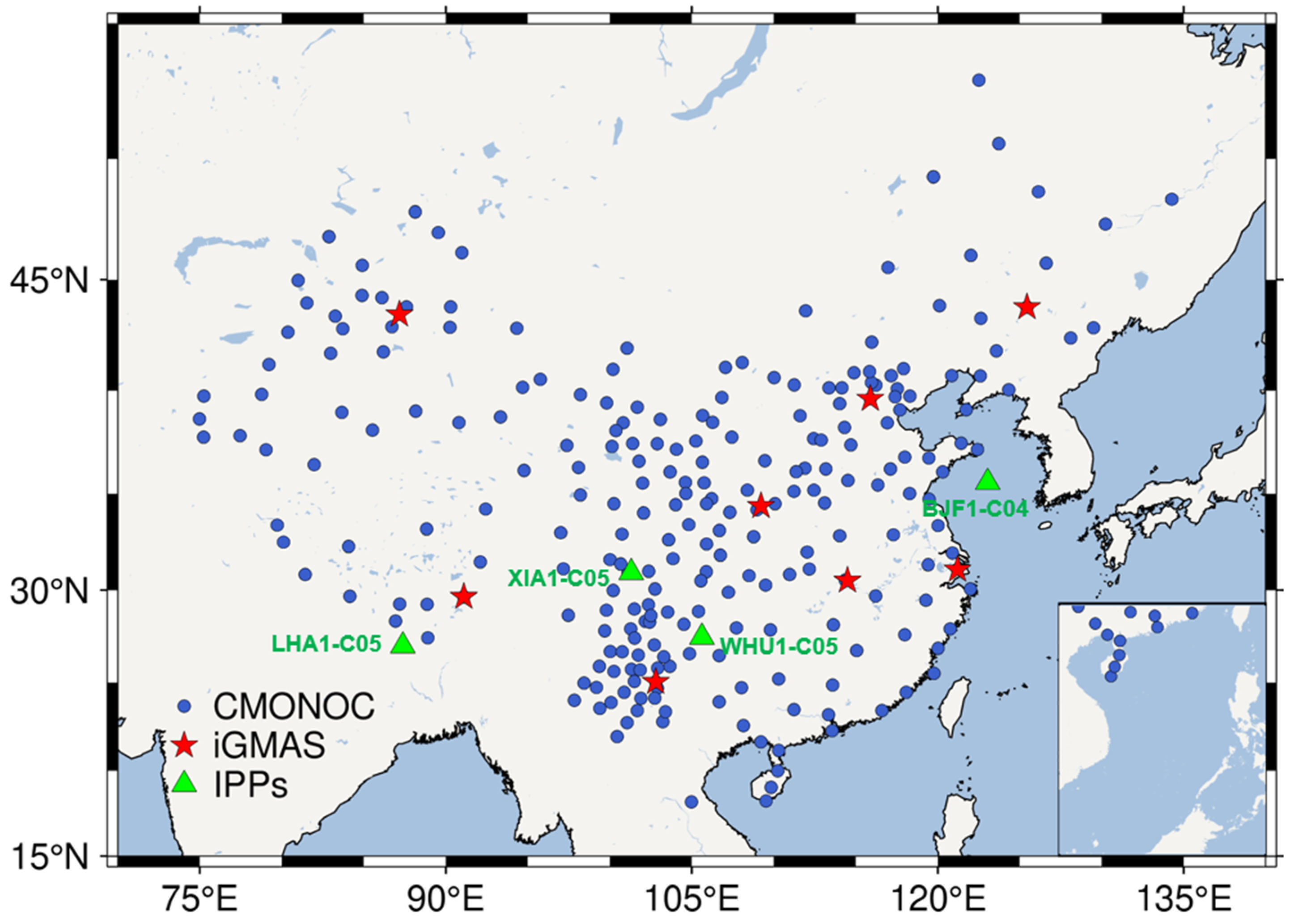
3.1. Data Sources and Station Distribution

We chose observations from 251 CMONOC stations and eight International GNSS Monitoring and Assessment System (iGMAS) stations to build the REIM model. The locations of GNSS stations and station-GEO IPPs are illustrated in Figure 1.

3.2. Geomagnetic Storm Classification and Experimental Dates Selection

The ionospheric TEC shows daily and seasonal periodic fluctuations driven by geomagnetic and solar activities. This study built the REIM model during a geomagnetic storm period when the ionosphere was more unstable. The disturbed period was chosen because it presents more challenges and is more valuable for assessing the reliability and positioning performance for real-time ionospheric modeling.

The Kp and Dst indices were utilized to measure the level of geomagnetic activity on Earth. The Kp index, which ranges from 0 to 9, represents the different intensities of geomagnetic activity, with higher values (e.g., 7 to 9) indicating greater intensity of geomagnetic activity. The Dst index, measured in nT, typically ranges from positive tens of nT to negative values exceeding −1000 nT. Geomagnetic storms are classified as strong when the Dst index falls between −200 nT and −100 nT. The classification of geomagnetic storms is shown in

Table 1. Geomagnetic storm level classification [23].

Storm Class:	Kp	Dst/nT
Weak	40	−50 < Dst ≤ −30
Moderate	50	−100 < Dst ≤ −50
Strong	7−	−200 < Dst ≤ −100
Severe	8+	−350 < Dst ≤ −200
Great	9−	Dst ≤ −350

[23]. In this study, experiment data were selected from a 7-day period from 23 August 2018 to 29 August 2018, corresponding to days of year (DOYs) 235–241. Geomagnetic storm days were identified as those when the Dst index was below −100 nT for the majority of the day. Thus, 26 August 2018 (DOY 238), as shown in Figure 2, was determined as the geomagnetic storm day with the lowest Dst dropping below −150 and the highest Kp exceeding 6.

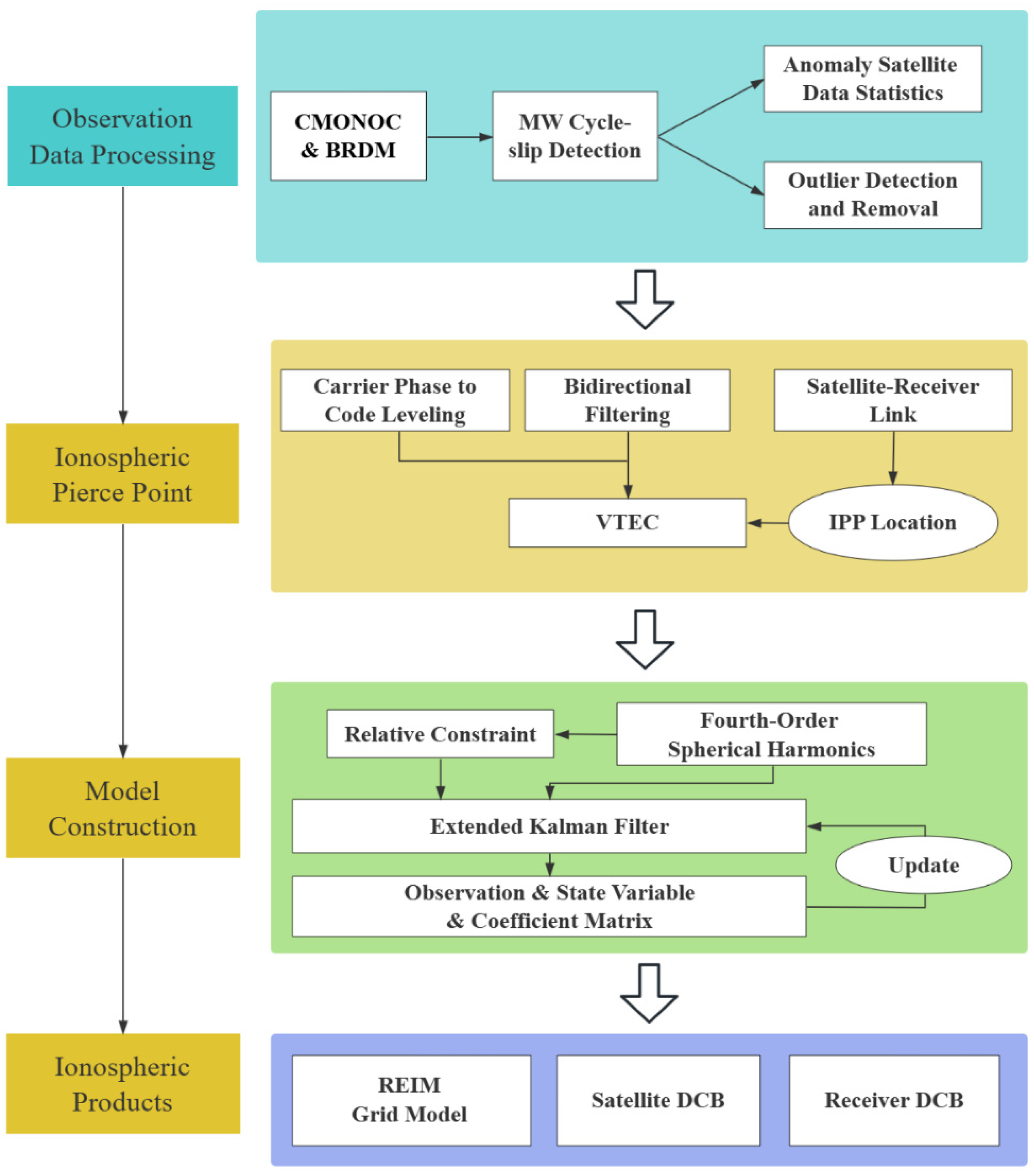
3.3. Modeling Strategies and Processing Workflow

Table 2. Characteristic of different ionospheric models, where the IOSR is provided by the China Earthquake Administration, the IGSG is the final GIM from IGS, and the CODG is the final GIM from CODE.

Model Products	TEC Extraction Methods	Modeling Methods	Temporal Resolution	Spatial Resolution	Range	Types
IGSG	Weighting of products from various analysis centers		2 h	2.5° × 5°	Global	Post-processing
CODG	Carrier phase to code leveling (CCL)	SH	1 h/2 h	2.5° × 5°	Global	Post-processing
IOSR	CCL	SH	1 h	1° × 1°	Regional	Post-processing
REIM	CCL	SH	1 h	1° × 1°	Regional	Real-time

presents the methods of TEC calculation and modeling, spatiotemporal resolutions, and coverage areas of the REIM model compared with other post-processed models. The REIM is a grid model fitted using a fourth-order spherical harmonic (SH) function, and the modeling parameters are estimated by the EKF in five-minute intervals. The settings for the modeling are detailed in

Table 3. REIM modeling settings, where the elevation mask refers to the minimum elevation angle of the satellites.

Items	Settings
Satellite systems	BDS, GPS, GLONASS
Data pre-processing	Cycle-slip detection, CCL
Elevation mask	10°
Sampling rate	30 s
Ephemeris type	Broadcast
Ionospheric modeling method	Fourth-order SH

, and the real-time modeling workflow is depicted in Figure 3.

4. Experimental Analyses

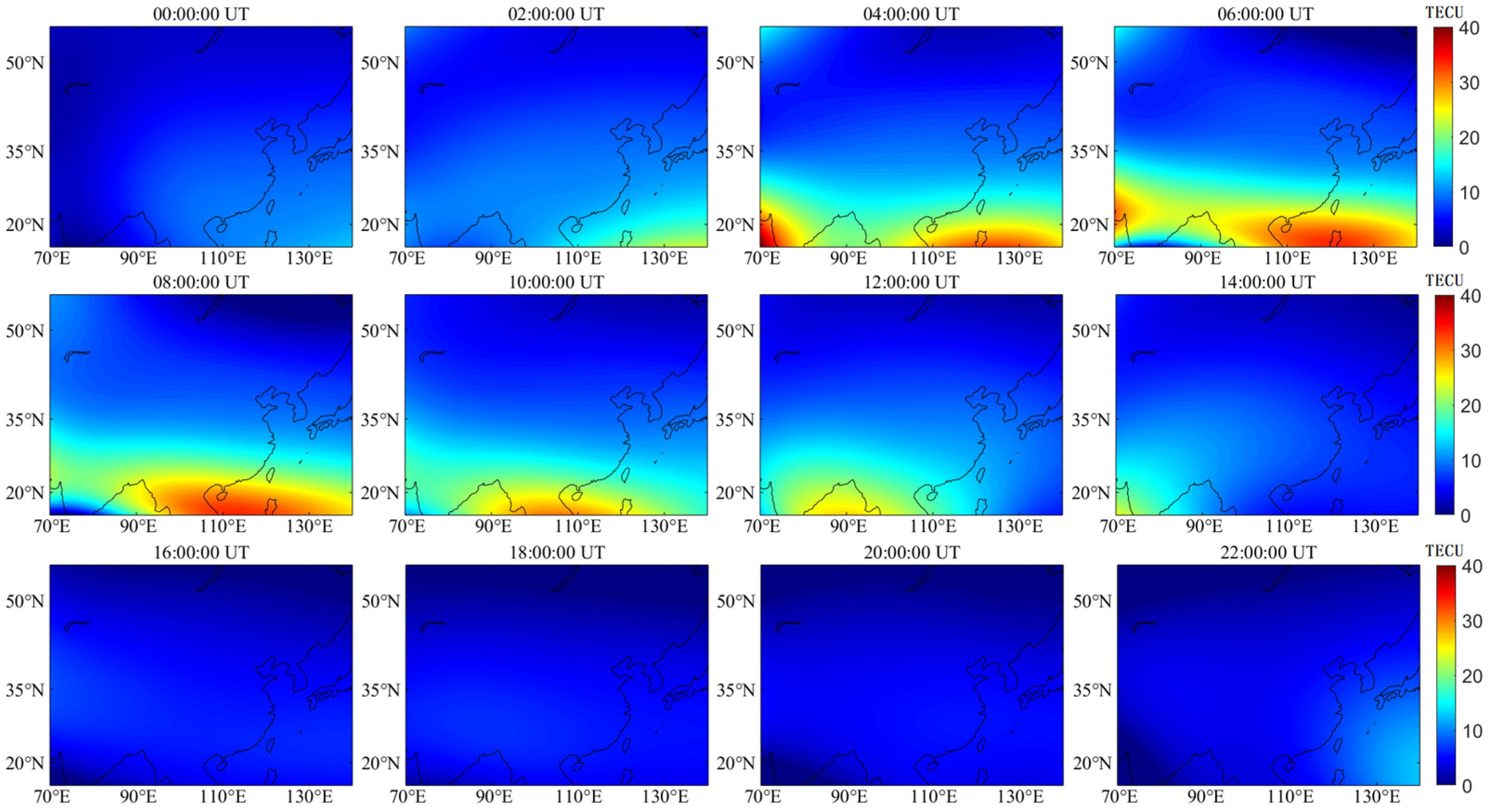
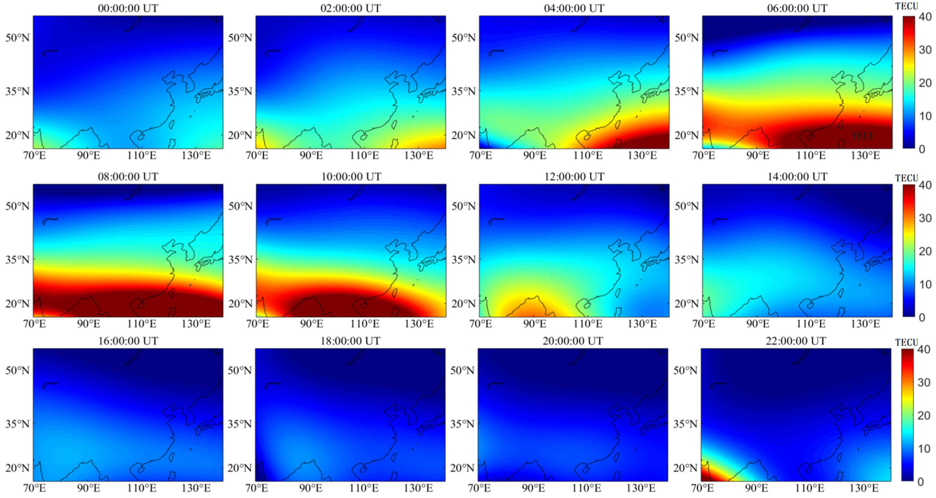
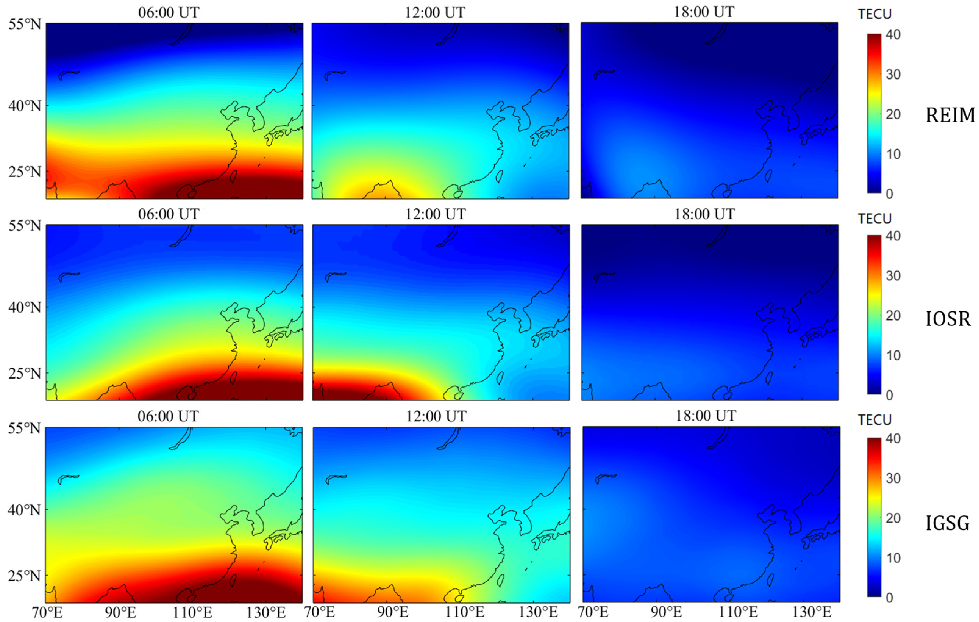
4.1. Spatial and Temporal Variations of VTEC

The ionospheric TEC periodically varies between day and night, corresponding to changes in solar radiation. During the daytime, ionospheric electron density and TEC increase as solar radiation intensifies, while at night, they decrease with the weakening solar radiation. Moreover, the levels of electron density and TEC vary with latitude. Regions near the equator usually show the highest levels of electron density and TEC because of the greatest concentration of solar radiation; meanwhile, lower latitudes show higher levels.

Figure 4 and Figure 5, respectively, present the VTEC variation maps of DOY 235 (magnetostatic) and DOY 238 (geomagnetic storm) calculated using the REIM model. The time labels are in UT, corresponding to UT+8 h at local (Beijing) time. The figures show that on both days, ionospheric VTECs increase with the intensification of solar radiation during the day and decrease with the weakening of solar radiation at night. In terms of spatial distribution, the variation in low-latitude regions is significantly higher than in high-latitude regions, and the VTEC fluctuations on the geomagnetic storm day (DOY 238) are significantly larger than those on the magnetostatic day (DOY 235). These results confirm that the REIM model is consistent with the general spatial and temporal characteristics of ionospheric VTEC.

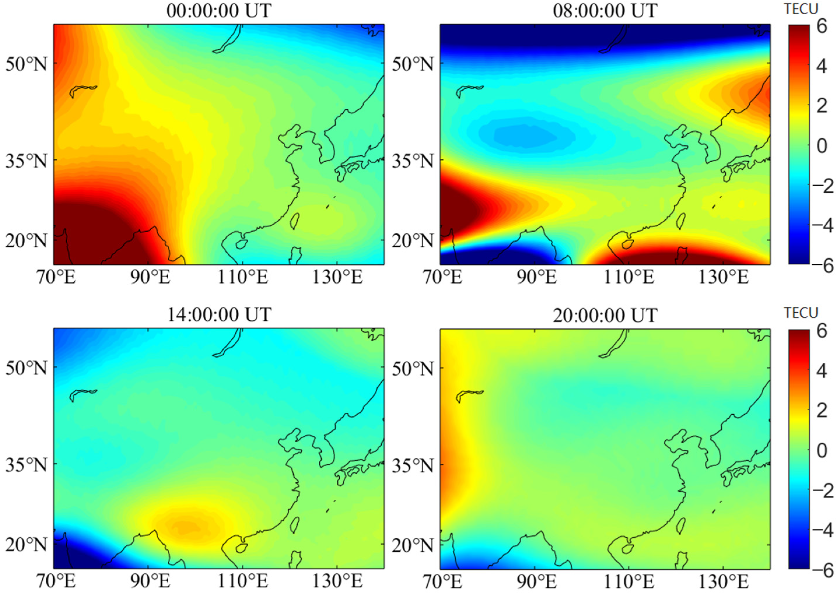
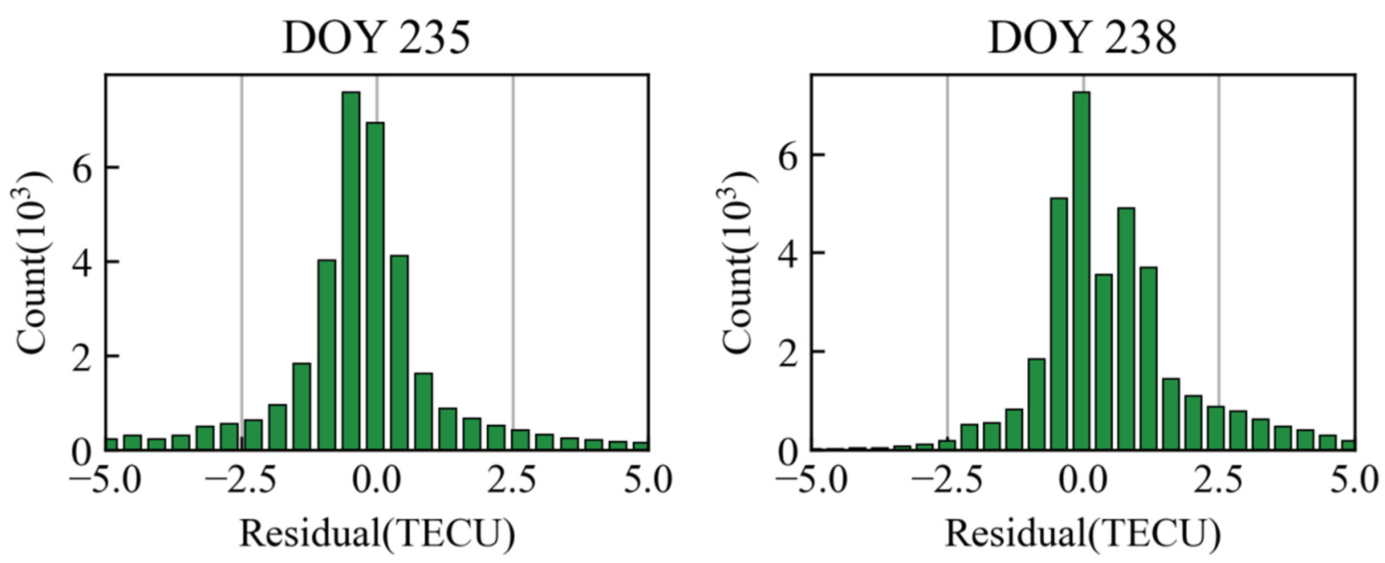
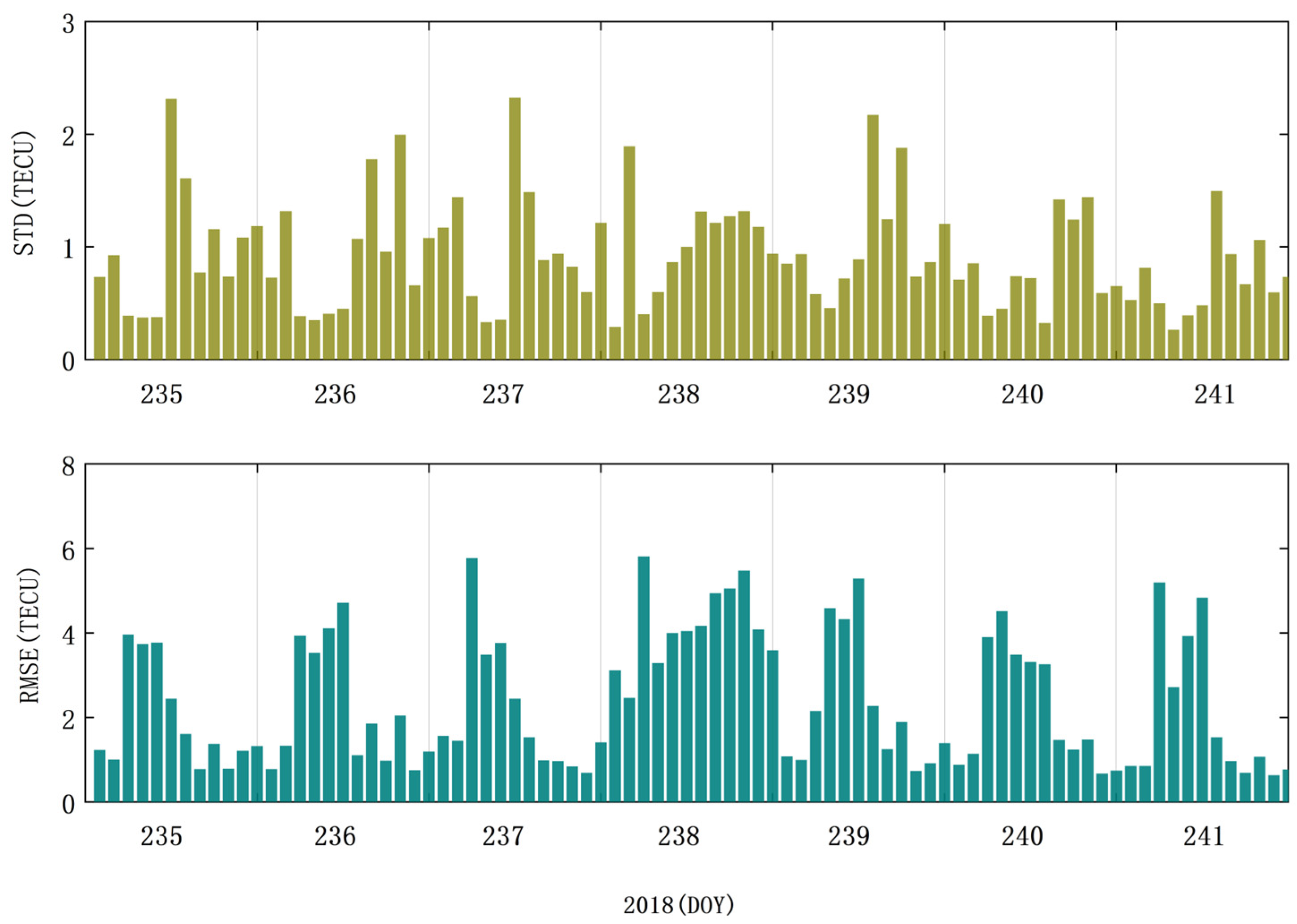
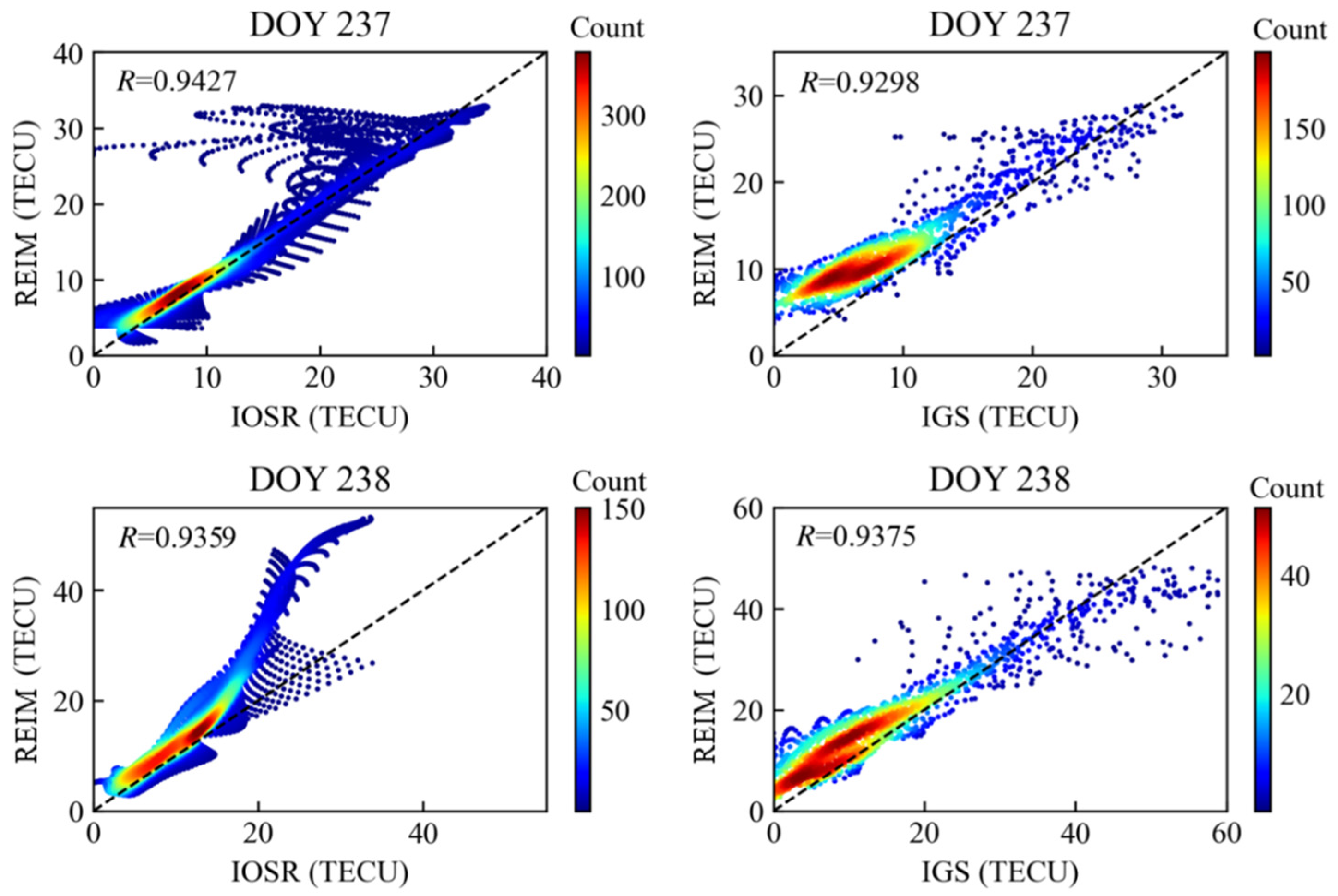
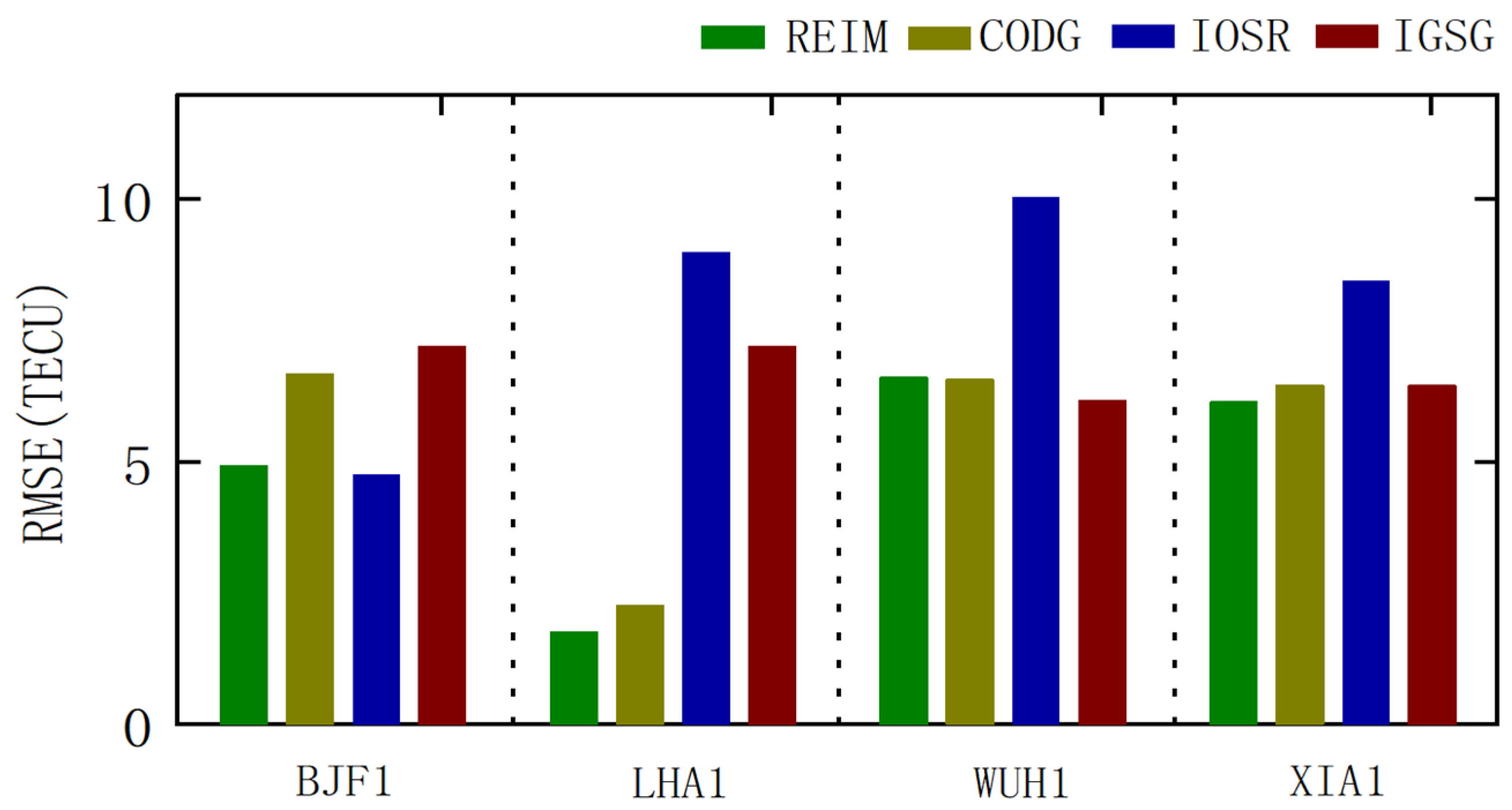
4.2. Consistency Analysis with Post-Processing Models

To assess the reliability of the REIM model, VTEC variations maps at 6 h intervals of the geomagnetic storm day (DOY 238) were generated using post-processed ionospheric products from different analysis centers, and the maps were compared. The results are shown in Figure 6. From the figure, it can be seen that all three models show the most significant VTEC variations at 6:00 UT and the greatest values in the region south of 25°N, reaching up to 40 TECU. This aligns with the known temporal and spatial distribution patterns of the ionosphere. The comparison indicates that VTECs calculated using the REIM model are consistent with the post-processing GIMs in both pattern and magnitude, demonstrating the reliability of the REIM model in effectively monitoring the ionospheric TEC variations.

To further compare the REIM model and post-processed ionospheric products, the VTEC differences between the REIM and IOSR models were plotted at four epochs (0:00, 8:00, 14:00, and 20:00 UT) for DOY 238, as shown in Figure 7. The overall VTEC differences are generally smaller than 6 TECU, with values even lower in the inland region of China, where differences are less than 2 TECU. This demonstrates a high level of consistency with post-processed products. What is more, due to its higher spatial resolution, the REIM model performs better than IGSG in capturing the VTEC gradient and is closer to the IOSR model, particularly in mid-latitude regions. It should be noted that the differences at the boundary regions are slightly larger, indicating a boundary effect. This can be attributed to the fact that CORS stations are mainly distributed in the inland areas of China, with few and unevenly distributed stations in the Tibet and South Asia regions, leading to significant VTEC differences for these areas. Two statistical histograms of VTEC differences between the REIM and IOSR for DOY 235 and DOY 238 are respectively presented in Figure 8. The histograms show that for both days, over 94% of the differences are less than 2.5 TECU, and the VTEC differences follow a normal distribution and are relatively concentrated. These results verify that the REIM model is highly consistent with the post-processed high-precision GIM products, further confirming the reliability of the REIM model.

The accuracy of the REIM model was then examined using the indices of root-mean-square error (RMSE) and standard deviation (STD). We calculated REIM-VTEC’s STD and RMSE referred to IOSR as Equation (9) and Equation (10), respectively:

$$STD=\sqrt{{\displaystyle \frac{1}{n}}\cdot {\displaystyle \sum _{i=1}^{\mathrm{n}}{(TE{C}_i^d-\overline{TE{C}^d})}^2}},$$

(9)

$$\mathrm{RMSE}=\sqrt{{\displaystyle \frac{1}{n}}\cdot {({\displaystyle \sum _{i=1}^{n}TE{C}_i^R-TE{C}_i^I})}^2},$$

(10)

where $TE{C}^d$ is the TEC difference between the two models, $TE{C}_i^R$ and $TE{C}_i^I$ are TEC values at different grid points derived from REIM and IOSR, respectively.

The STD and RMSE bar graphs over the seven days from DOY 235 to DOY 241 are shown in Figure 9. STD reflects the degree of data dispersion, while RMSE indicates the differences between estimations and “true” values. As Figure 9 shows, the STDs are predominantly below 2 TECU during the seven days and more stable on DOY 238 (geomagnetic storm day), with values maintained around 1 TECU. The RMSE bar graph shows overall values within 5 TECUs, with slightly higher values on DOY 238, reaching approximately 4 TECUs throughout the day. Meanwhile, the mean deviation of DOY 238 is 0.97 TECU, which is lower than that on magnetic quiet days. The results of STD and RMSE demonstrate small differences from the post-processed GIM products and high stability of the REIM model during the investigated period.

Correlation indicators are used to quantify the degree of proximity between two variables. In this study, the VTEC coefficient of determination (R²), which ranges from 0 to 1, was selected to assess the correlation between the REIM and post-processing models. Figure 10 shows the coefficient of determination between the REIM model and the IOSR, as well as the IGSG post-processing models on DOY 237 and DOY 238. On DOY 237, the R between the REIM model and the IOSR model is 0.94, and that between the REIM and IGSG model is 0.93. On DOY 238, the R value is 0.94 with the IOSR model and 0.94 with the IGSG model, respectively. The high R values indicate strong correlations with both IOSR and IGSG models, even during the geomagnetic storm period. This confirms that the REIM model can achieve a high level of agreement with post-processing products, demonstrating its capability to provide reliable real-time estimation of ionospheric TECs in the region of China.

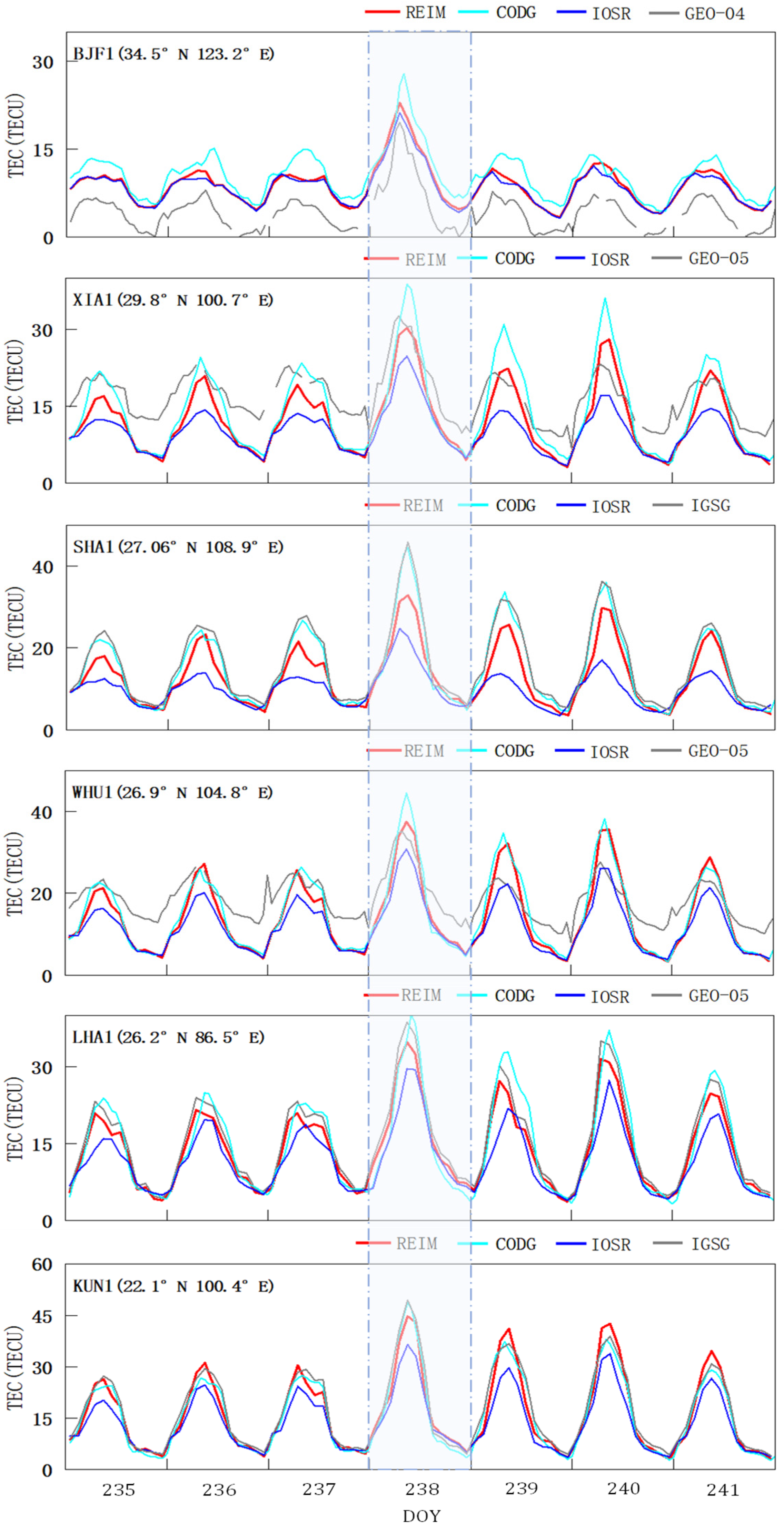
4.3. Consistency Analysis with BDS GEO Satellites

BDS GEO satellites are characterized by their relatively fixed positions relative to the Earth’s surface. Accordingly, the IPPs between GEO satellites and ground-based stations remain almost unchanged. This stability provides a good opportunity for long-term monitoring of TEC variations at these IPPs. We derived the VTECs from the REIM model and other post-processed models at the IPPs of BDS GEO satellites, and their deviations from VTECs were calculated using the GEO satellite observations, which are shown in Figure 11. The corresponding RMSE are presented in Figure 12, while the mean deviations are in

Table 4. VTEC deviation between different ionospheric models and BDS GEO satellites at four stations (unit: TECU).

Models	Stations
	BJF1	LHA1	WUH1	XIA1	Mean
REIM	4.32	2.79	4.93	4.58	4.15
CODG	5.57	2.88	5.23	5.06	4.68
IOSR	4.41	6.74	7.45	6.51	6.27
IGSG	6.23	6.21	5.09	5.14	5.67

. Six GNSS stations in China are equipped with receivers for BDS GEO satellites: BJF1, KUN1, LHA1, WHU1, SHA1, and XIA1. However, due to anomalies at KUN1 and SHA1 during this period, only observations of the remaining four stations were used for comparison in this study.

As shown in Figure 11, the peak VTECs of all models on each day are highly consistent with VTECs of BDS GEO observations, with a relatively lower peak of the IOSR model. On the geomagnetic storm day, August 26 (DOY 238), VTECs from these models show increased consistency, with small differences from the BDS GEO measurements. It should be noted that the GEO VTEC observations obtained from BJF1 exhibit relatively lower overall values. Considering the same VTEC extraction method, we attribute this anomaly to two main factors: (1) The BJF1 station has a higher latitude and selected GEO-C04 rather than C05, which amplifies projection function errors due to the lower satellite elevation angles and potentially introduces discrepancies in satellite data quality. (2) The station-GEO IPPs plot (Figure 1) indicates that only the BJF1-C04 IPP is located above the East China sea. It means that all GIMs must extrapolate the VTEC at this point, which further exacerbates the difference between GEO VTEC and GIM VTEC. In general, the VTEC values from the REIM and CODG models are more closely aligned with the reliable BDS GEO measurements, while the IOSR model exhibits a larger difference.

Figure 12 shows the RMSE statistics of VTECs from the ionospheric models, providing more details to analyze the VTEC deviation of each model from BDS GEO observations. Among the four GNSS stations, the models show the smallest deviation at BJF1. The VTEC RMSE values between BDS GEO and the REIM, CODG, IOSR, and IGSG models range from 2–6 TECU, 2.5–6 TECU, 5–10 TECU, and 5.5–7 TECU, respectively. The REIM model exhibits the smallest RMSE compared with other models, whereas the IOSR model shows the largest RMSE. The comparison with BDS GEO observations demonstrates that the REIM model has greater stability and higher precision than post-processing GIM products during the geomagnetic period discussed in this study.

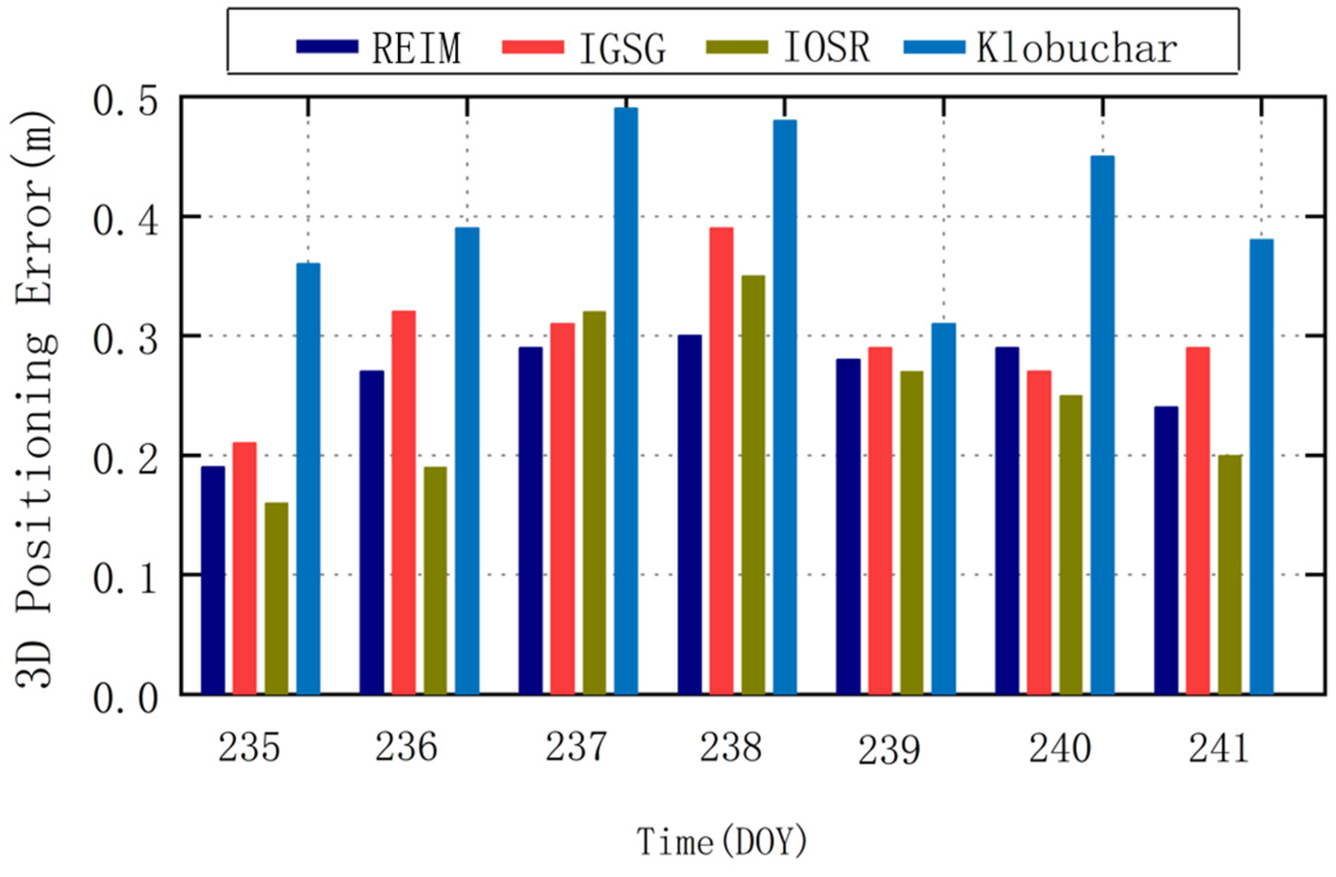
4.4. Assessment in RT-SF-PPP

To further evaluate the performance of the REIM model, we applied it to ionospheric delay correction in RT-SF-PPP. The four GNSS stations used in the comparison with the BDS GEO observations were selected for this experiment. The RT-SF-PPP convergence performances of the REIM and IGSG models were first compared, and the findings are shown in Figure 13. Then, the average 3D positioning errors for the REIM, IGSG, IOSR, and Klobuchar models during the investigated period were statistically analyzed, as depicted in Figure 14.

In PPP, convergence time refers to the duration from when the receiver is activated until it achieves the expected real-time positioning accuracy. As shown in Figure 13, convergence is achieved within 80 epochs with an error of 0.1 m in all three directions when applying the REIM model for ionospheric error correction, while approximately 140 epochs are required when using the IGSG model. The convergence speed is significantly faster when correcting ionospheric delay using the REIM model compared with the IGSG product in RT-SF-PPP. The average positioning errors in the three directions for each day using different models are illustrated in Figure 14. The bar graphs indicate that the 3D positioning errors in RT-SF-PPP are at the level of decimeters for all models. The Klobuchar model shows the poorest correction with positioning error between 0.3 m and 0.5 m. This is reasonable, as it is a broadcast empirical model. By contrast, the positioning errors in SF-PPP with ionospheric delay correction using the REIM, IGSG, and IOSR models range from 0.16 m to 0.39 m. Among the three models, the IOSR model leads to the smallest 3D positioning, followed by the REIM model.

The average positioning errors of SF-PPP in East (E), North (N), and Up (U) directions with ionospheric delay correction using different models are presented in

Table 5. Statistics of positioning errors in three directions obtained by different ionospheric models (unit: m).

Models	Directions
	East	North	Up
REIM	0.086	0.116	0.301
IGSG	0.095	0.129	0.322
IOSR	0.053	0.091	0.290
Klobuchar	0.098	0.129	0.582

. It can be found that the errors in the E direction are the smallest for all ionospheric models. In the N direction, the IOSR model achieves the smallest error with the value of 0.091 m at the centimeter level, while the other models only achieve positioning errors at decimeter level. In the U direction, positioning errors for all models are at the decimeter level, with values of 0.301 m, 0.322 m, 0.290 m, and 0.582 m for the REIM, IGSG, IOSR, and Klobuchar models, respectively. The IOSR model demonstrates the smallest poisoning errors in all three directions, followed by the REIM model. The ionospheric delay correction using the Klobuchar model is significantly weaker than the others in the U direction. This experiment indicates that the performance of the REIM model in SF-PPP ionospheric delay correction is comparable to that of the high-precision post-processing ionospheric models.

5. Conclusions

Real-time ionospheric TEC modeling, as a critical technique for ionospheric delay correction, is very important for improving the precision and reliability of real-time GNSS positioning. This study integrates the EKF algorithm into the real-time ionospheric TEC modeling to develop the REIM model over China using GNSS observations from CMONOC and iGMAS. A 7-day period around the geomagnetic storm in August 2018 was selected for modeling and validation in this study. The accuracy, reliability, and performance of the REIM model were examined by comparing it with multiple post-processing ionospheric models from different GNSS analysis centers, measurements from BDS GEO satellites, and the RT-SF-PPP experiment.

The spatial and temporal characteristics of the REIM-modeled ionospheric TECs were first analyzed and compared. The mean deviation between the REIM and IOSR models was 0.97 TECU, with corresponding RMSE of 1–4 TECU and STD of 0.5–2.5 TECU. The REIM model exhibited a strong correlation with post-processing ionospheric models, with a correlation coefficient of 0.9359 between REIM and IOSR and 0.9375 between REIM and IGSG. In the VTEC consistency analysis with BDS GEO measurements at IPPs, the REIM model demonstrated higher consistency. The mean deviations of REIM, CODG, IOSR, and IGSG were 4.15, 4.68, 6.23 and 5.67 TECU, respectively, with corresponding RMSEs of 5.12, 5.75, 7.21 and 6.28 TECU.

In the RT-SF-PPP ionospheric delay correction experiment, the convergence times using the REIM and IGSG models were 80 epochs and 140 epochs, respectively. The positioning errors in the East direction for SF-PPP were 0.086 m, 0.095 m, 0.053 m, and 0.098 m for the REIM, IGSG, IOSR, and Klobuchar models, respectively. In conclusion, the REIM model can lead to faster convergence compared with the IGS final product in RT-SF-PPP, provides higher precision ionospheric delay correction than the Klobuchar broadcast model, and offers comparable accuracy to high-precision post-processing models.

References

1. Li, Z.; Wang, N.; Wang, L.; Liu, A.; Yuan, H.; Zhang, K. Regional ionospheric TEC modeling based on a two-layer spherical harmonic approximation for real-time single-frequency PPP. J. Geod. 2019, 93, 1659–1671. [Google Scholar] [CrossRef]
2. Macalalad, E.P.; Tsai, L.-C.; Wu, J.; Liu, C.-H. Application of the Taiwan Ionospheric Model to single-frequency ionospheric delay corrections for GPS positioning. GPS Solut. 2012, 17, 337–346. [Google Scholar] [CrossRef]
3. Jin, X.; Song, S. Near real-time global ionospheric total electron content modeling and nowcasting based on GNSS observations. J. Geod. 2023, 97, 27. [Google Scholar] [CrossRef]
4. Feltens, J. Development of a new three-dimensional mathematical ionosphere model at European Space Agency/European Space Operations Centre. Space Weather 2007, 5, 12002. [Google Scholar] [CrossRef]
5. Li, Z.; Yuan, Y.; Wang, N.; Hernandez-Pajares, M.; Huo, X. SHPTS: Towards a new method for generating precise global ionospheric TEC map based on spherical harmonic and generalized trigonometric series functions. J. Geod. 2014, 89, 331–345. [Google Scholar] [CrossRef]
6. Schaer, S.; Gurtner, W.; Feltens, J. IONEX: The ionosphere map exchange format version 1. In Proceedings of the IGS AC Workshop, Darmstadt, Germany, 25 February 1998; pp. 225–232. [Google Scholar]
7. Hernández-Pajares, M.; Juan, J.M.; Sanz, J. High resolution TEC monitoring method using permanent ground GPS receivers. Geophys. Res. Lett. 1997, 24, 1643–1646. [Google Scholar] [CrossRef]
8. Li, Z.; Wang, N.; Hernández-Pajares, M.; Yuan, Y.; Krankowski, A.; Liu, A.; Zha, J.; García-Rigo, A.; Roma-Dollase, D.; Yang, H. IGS real-time service for global ionospheric total electron content modeling. J. Geod. 2020, 94, 32. [Google Scholar] [CrossRef]
9. Hernández-Pajares, M.; Juan, J.M.; Sanz, J.; Orus, R.; Garcia-Rigo, A.; Feltens, J.; Komjathy, A.; Schaer, S.C.; Krankowski, A. The IGS VTEC maps: A reliable source of ionospheric information since 1998. J. Geod. 2009, 83, 263–275. [Google Scholar] [CrossRef]
10. Zhu, F.; Yang, J.; Qing, Y.; Li, X. Assessment and analysis of the global ionosphere maps over China based on CMONOC GNSS data. Front. Earth Sci. 2023, 11, 1095754. [Google Scholar] [CrossRef]
11. Fuller-Rowell, T.; Araujo-Pradere, E.; Minter, C.; Codrescu, M.; Spencer, P.; Robertson, D.; Jacobson, A.R. US-TEC: A new data assimilation product from the Space Environment Center characterizing the ionospheric total electron content using real-time GPS data. Radio Sci. 2006, 41, 1–8. [Google Scholar] [CrossRef]
12. Wübbena, G.; Schmitz, M.; Bagge, A. Real-Time GNSS Data Transmission Standard RTCM 3.0. In Proceedings of the Geo++® GmbH IGS Workshop, Darmstadt, Germany, 8–12 May 2006. [Google Scholar]
13. Chen, P.; Liu, H.; Schmidt, M.; Yao, Y.; Yao, W. Near real-time global ionospheric modeling based on an adaptive Kalman filter state error covariance matrix determination method. IEEE Trans. Geosci. Remote Sens. 2021, 60, 5800812. [Google Scholar] [CrossRef]
14. Erdogan, E.; Schmidt, M.; Seitz, F.; Durmaz, M. Near real-time estimation of ionosphere vertical total electron content from GNSS satellites using B-splines in a Kalman filter. Ann. Geophys. 2017, 35, 263–277. [Google Scholar] [CrossRef]
15. Bilitza, D.; McKinnell, L.-A.; Reinisch, B.; Fuller-Rowell, T. The international reference ionosphere today and in the future. J. Geod. 2011, 85, 909–920. [Google Scholar] [CrossRef]
16. Klobuchar, J.A. Ionospheric time-delay algorithm for single-frequency GPS users. IEEE Trans. Aerosp. Electron. Syst. 1987, 23, 325–331. [Google Scholar] [CrossRef]
17. Chen, J.; Xiong, P.; Wu, H.; Zhang, X.; Feng, J.; Zhang, T. A Multi-Parameter Empirical Fusion Model for Ionospheric TEC in China’s Region. Remote Sens. 2023, 15, 5445. [Google Scholar] [CrossRef]
18. He, R.; Li, M.; Zhang, Q.; Zhao, Q. A Comparison of a GNSS-GIM and the IRI-2020 Model Over China Under Different Ionospheric Conditions. Space Weather 2023, 21, e2023SW003646. [Google Scholar] [CrossRef]
19. Srivani, I.; Prasad, G.S.V.; Ratnam, D.V. A deep learning-based approach to forecast ionospheric delays for GPS signals. IEEE Geosci. Remote Sens. Lett. 2019, 16, 1180–1184. [Google Scholar] [CrossRef]
20. Pan, Y.; Jin, M.; Zhang, S.; Deng, Y. TEC Map Completion Using DCGAN and Poisson Blending. Space Weather 2020, 18, e2019SW002390. [Google Scholar] [CrossRef]
21. Ruwali, A.; Kumar, A.J.S.; Prakash, K.B.; Sivavaraprasad, G.; Ratnam, D.V. Implementation of Hybrid Deep Learning Model (LSTM-CNN) for Ionospheric TEC Forecasting Using GPS Data. IEEE Geosci. Remote Sens. Lett. 2020, 18, 1004–1008. [Google Scholar] [CrossRef]
22. Guo, D.; Wang, X.; Chen, R. New sequential Monte Carlo methods for nonlinear dynamic systems. Stat. Comput. 2005, 15, 135–147. [Google Scholar] [CrossRef]
23. Loewe, C.A.; Prölss, G.W. Classification and mean behavior of magnetic storms. J. Geophys. Res.-Space 1997, 102, 14209–14213. [Google Scholar] [CrossRef]
Figure 1. Location of GNSS stations, where blue points represent CMONOC stations, red pentagrams represent iGMAS stations, and green triangles represent station-GEO IPPs locations.
Remotesensing 17 01568 g001
Figure 2. Fluctuations of Kp and Dst indices during DOY 235 to DOY 241.
Remotesensing 17 01568 g002
Figure 3. Real-time modeling workflow of the REIM model, where BRDM refers to the multi-system broadcast ephemeris file provided by IGS, and MW refers to the Melbourne–Wübbena combination method.
Remotesensing 17 01568 g003
Figure 4. VTEC variations on DOY 235 of the REIM model with a 2 h interval.
Remotesensing 17 01568 g004
Figure 5. VTEC variations on DOY 238 of the REIM model with a 2 h interval.
Remotesensing 17 01568 g005
Figure 6. Comparison of different models at 6 h intervals on DOY 238.
Remotesensing 17 01568 g006
Figure 7. VTEC difference between REIM and IOSR at different moments on DOY 238.
Remotesensing 17 01568 g007
Figure 8. Statistics of VTEC differences between REIM and IOSR on DOY 235 and DOY 238.
Remotesensing 17 01568 g008
Figure 9. STD and RMSE histograms of REIM compared with IOSR during the investigated period.
Remotesensing 17 01568 g009
Figure 10. Correlation indicators of REIM with IOSR (left) and IGSG (right) on DOY 237 and DOY 238.
Remotesensing 17 01568 g010
Figure 11. VTEC obtained from ionospheric models and BDS GEO observations at the IPPs for the six stations during the investigated period.
Remotesensing 17 01568 g011
Figure 12. RMSE statistics for VTECs from ionospheric models referred to BDS GEO observations at four stations.
Remotesensing 17 01568 g012
Figure 13. 3D convergence effect utilizing the REIM model and the IGSG model.
Remotesensing 17 01568 g013
Figure 14. Three-dimensional positioning error results obtained from different ionospheric models.
Remotesensing 17 01568 g014