Article

Post-Processing Optimization of the Global 30 m Land Cover Dynamic Monitoring Product

1
Key Laboratory of Digital Earth Science, Aerospace Information Research Institute, Chinese Academy of Sciences, Beijing 100094, China
2
International Research Center of Big Data for Sustainable Development Goals, Beijing 100094, China
3
University of Chinese Academy of Sciences, Beijing 100049, China
4
College of Geomatics, Xi’an University of Science and Technology, Xi’an 710054, China
*
Author to whom correspondence should be addressed.
Remote Sens. 2025, 17(9), 1558; https://doi.org/10.3390/rs17091558
Submission received: 27 February 2025 / Revised: 13 April 2025 / Accepted: 26 April 2025 / Published: 27 April 2025

Abstract

:
Post-processing optimization refers to the refinement of land cover products by applying specific rules or algorithms to minimize erroneous changes in land cover types caused by classification uncertainty or interannual phenological variations. Global land cover (GLC) mapping has gained significant attention over the past decade, but current GLC time-series products suffer from considerable inconsistencies in mapping results between different epochs, leading to severe erroneous changes. Here, we aimed to design a novel post-processing approach by combining multi-source data to optimize the GLC_FCS30D product, which represents a groundbreaking improvement in GLC dynamic mapping at a resolution of 30 m. First, spatiotemporal filtering with a window size of 3 × 3 × 3 was applied to reduce the “salt-and-pepper” effect. Second, a temporal consistency optimization algorithm based on LandTrendr was used to identify land cover changes across the entire time series and eliminate excessively frequent erroneous changes. Third, certain land cover transitions between easily misclassified types were optimized using logical rules and multi-source data. Specifically, the illogical wetland-related transitions (wetland–water and wetland–forest) were corrected using a simple replacement rule. To address the noticeable erroneous changes in arid and semi-arid regions, the erroneous land cover transitions involving bare areas, sparse vegetation, grassland, and shrubland were corrected by combining NDVI and precipitation data. Finally, the performance of our post-processing optimization approach was evaluated and quantified. The proposed approach successfully reduced the cumulative change area from 7537.00 million hectares (Mha) in the GLC_FCS30D product without optimization to 1981.00 Mha in the GLC_FCS30D product with optimization, eliminating 5556.00 Mha of erroneous changes across 26 epochs. Furthermore, the overall accuracy of the mapping was also improved from 73.04% to 74.24% for the Land Cover Classification System (LCCS) level-1 validation system. Erroneous changes in GLC_FCS30D were considerably mitigated with the post-processing optimization method, providing more reliable insights into GLC changes from 1985 to 2022 at a 30 m resolution.

1. Introduction

Land cover products record the spatiotemporal dynamics of various surface features, such as vegetation, buildings, and water distribution, across different regions of the Earth’s surface [1,2,3,4]. Advancements in satellite remote sensing technology, as well as increases in computer storage and computational power, have led to the evolution of land cover mapping research from low-resolution to high-resolution products, and from single-period to multi-temporal annual products [5,6,7].
Despite these advances in the field, current multi-temporal global land cover products still exhibit considerable inconsistencies between different epochs, leading to a substantial number of erroneous changes (i.e., incorrect land cover changes) in change detection studies [8]. A key contributing factor to these inconsistencies is that most existing land cover products classify each epoch independently. Specifically, high-confidence training samples are selected for each epoch, and supervised classification models are used to independently extract classification results for each epoch. However, this approach, which classifies multi-temporal data independently for each epoch, may introduce geometric misregistration and large classification errors. These discrepancies can lead to inconsistent classification results across products from different periods, thereby generating a significant number of erroneous changes in change detection research. This ultimately reduces detection accuracy or renders the product unsuitable for change analysis [9,10].
Existing per-epoch classified land cover products are inadequate for supporting land cover change analysis. In contrast, the combination of continuous change detection and dynamic update are expected to provide a more accurate and precise understanding of global land cover changes. Land cover dynamic update products use change detection models to identify and extract changed pixels, while also employing unchanged pixels to train classification models for updating the changed pixels. This approach can enhance the temporal consistency between products from different epochs. For example, Xian et al. utilized Landsat satellite imagery and other auxiliary data to create the LCMAP product at a resolution of 30 m for the contiguous United States, using the continuous change detection and classification (CCDC) algorithm [11]. Similarly, Xie et al. combined the CCDC algorithm with the Markov random field (MRF) model to generate an annual land cover map for Beijing at a 30 m resolution from 2001 to 2020 [12]. Making use of the Google Earth Engine platform, Zhang et al. developed GLC_FCS30D, a global land cover dynamics monitoring product with a long time series and dynamic updates at 30 m, based on the CCDC algorithm and all available Landsat satellite imagery [13].
The original developers of the CCDC algorithm have noted that the method may exhibit issues in regions with significant interannual variations. For instance, semi-arid areas, where phenological processes experience large temporal fluctuations, may overestimate changes due to substantial spectral data variation at certain times of the year [14]. Similarly, the GLanCE product, developed by the National Aeronautics and Space Administration (NASA), also highlighted that the algorithm tends to overestimate land cover changes in semi-arid regions [15]. Moreover, a previous study has shown that the CCDC algorithm is overly sensitive when detecting forest changes, resulting in fragmented outputs [16]. To enhance the consistency and accuracy of the GLC_FCS30D product, post-processing optimization is necessary to improve the precision and reliability of change monitoring. This is an urgent task of great significance for the application of GLC_FCS30D in various fields [17,18].
Currently, numerous post-processing methods have been developed for land cover products [19,20,21], which can generally be categorized into two major types: (1) methods independent of spatiotemporal information, and (2) methods dependent on spatiotemporal information. The fundamental difference between these two approaches lies in whether they incorporate the spatial and temporal contextual information of the land cover data for correction and optimization. Post-processing methods that do not rely on spatiotemporal information primarily depend on expert knowledge or prior rules to impose constraints and adjustments on land cover classification results, without considering temporal or spatial relationships between pixels. The main idea of these methods is to eliminate or correct implausible transition patterns or obvious classification errors after the initial classification process, thereby reducing noise and misclassification [22,23]. In contrast, spatiotemporally dependent optimization methods have gained increasing attention in recent years. These approaches typically utilize statistical models or mathematical algorithms in combination with spatial and temporal contextual information to refine the classification results of target pixels [24,25]. For example, the spatiotemporal filtering algorithm calculates the probability of a central pixel’s type occurring in a surrounding 3 × 3 × 3 spatiotemporal window. A low probability suggests the pixel is likely misclassified, while a high probability indicates correct classification [26,27]. However, current research on post-processing optimization faces several limitations and shortcomings. For instance, long-time-series information is often underutilized, and most studies focus on classification post-processing in local time periods. Furthermore, only a few studies have effectively integrated multi-source data for optimization.
In this study, we aim to conduct post-processing optimization to address the issue of erroneous changes in the time-series GLC_FCS30D dataset by combining multi-source data, including remote sensing data, meteorological data, and logical rules, and to generate an improved version of the GLC_FCS30D product with enhanced spatiotemporal consistency. The post-processing optimization primarily focuses on four aspects: (1) spatiotemporal filtering; (2) a temporal consistency optimization algorithm based on LandTrendr; (3) optimization of wetland-related land cover transitions through simple logical rules; and (4) optimization of bare areas, sparse vegetation, grassland, and shrubland cover types in arid and semi-arid regions by combining the time-series normalized difference vegetation index (NDVI) data with precipitation data.

2. Materials and Methods

2.1. Materials

2.1.1. GLC_FCS30D Dataset

The GLC_FCS30D dataset represents a trailblazing improvement in global land cover monitoring, offering comprehensive insights into land cover dynamics at a resolution of 30 m, spanning the period from 1985 to 2022. Developed using dense time-series Landsat imagery and the continuous change detection method within the Google Earth Engine platform, GLC_FCS30D consists of 35 land cover subcategories with 26 epochs. Updates were made every five years prior to 2000 and annually thereafter. The overall accuracy (O.A.) of GLC_FCS30D in 2020 was 80.88% (±0.27%) for the 10 major land cover types within the basic classification system and 73.04% (±0.30%) for the Land Cover Classification System (LCCS) level-1 validation system. Additionally, the mean O.A. of GLC_FCS30D from 1985 to 2018 was 79.50% (±0.50%) in the contiguous United States (CONUS) based on the LCMAP_Val annual validation dataset. Additionally, its mean O.A. was 81.91% (±0.09%) from 2006 to 2018 across the European Union (EU) based on the LUCAS validation dataset [13]. The correspondence between the 35 fine land cover types in GLC_FCS30D and the basic classification system (10 major land cover types), as well as the LCCS level-1 validation system (17 land cover types), is presented in Table A1 [13,28,29]. The GLC_FCS30D dataset is available at https://zenodo.org/records/8239305 (accessed on 21 February 2025).
However, the complexity of the Earth system and the inherent uncertainties in quantitative remote sensing mapping can lead to over-detection in the GLC_FCS30D product. This is a result of limitations in the algorithms used for production and satellite image processing. Such over-detection results in a large number of erroneous changes in the GLC_FCS30D product, particularly in two cases: first, random erroneous changes can occur in both temporal and spatial domains; second, in wetland-related cover types and arid and semi-arid regions, there can be notable seasonal and interannual variations in surface cover, even though the land cover and land use remain unchanged.

2.1.2. Validation Datasets

In this study, we use three validation datasets that were originally employed for the release of the GLC_FCS30D product to evaluate the precision of the optimized product. This comparison allows for an intuitive evaluation of the impact of post-processing optimization. The three validation datasets are as follows: (1) 84,526 globally distributed validation samples in 2020; (2) LCMAP_Val, which includes 27,000 validation samples from the CONUS at a resolution of 30 m, covering the period from 1985 to 2021; and (3) LUCAS, which includes 1,090,863 validation samples from the EU, with 3-year intervals from 2006 to 2018. All three validation datasets have undergone measures to ensure quality and reliability, as detailed in previous work [13,30,31,32]. The second and third validation datasets are available at https://www.usgs.gov/special-topics/lcmap/validation-data (accessed on 21 February 2025) and https://esdac.jrc.ec.europa.eu/projects/lucas (accessed on 21 February 2025). The classification system for the 84,526 validation samples in 2020 follows the LCCS level-1 validation system. Table A2 illustrates the correspondence between the fine classification system of the GLC_FCS30D product and the 8 land cover classifications of LUCAS and the 8 land cover classifications of LCMAP.

2.1.3. Global Aridity Index Dataset

The Global Aridity Index and Potential Evapotranspiration Database: Version 3 provides high-resolution (30 arc seconds) global hydroclimatic data for monthly and annual averages (1970–2000). The dataset is based on the FAO Penman–Monteith reference evapotranspiration (ET0) equation, offering a robust tool for various scientific applications in light of the rapidly changing climate conditions [33]. For this study, only the annual average aridity index product from this database was utilized, and the dataset is available at https://cgiarcsi.community (accessed on 21 February 2025).

2.1.4. Landsat 5, Landsat 7, and Landsat 8 Satellite Images

The Landsat series of satellites have been continuously observing Earth’s surface since 1972, capturing multispectral and thermal data globally at a 30 m resolution approximately every two weeks [34,35]. In this study, surface reflectance data from the TM sensor of Landsat 5, the ETM+ sensor of Landsat 7, and the OLI/TIRS sensor of Landsat 8 were used to synthesize the NDVI.

2.1.5. ERA5-Land Precipitation Data

The European Centre for Medium-Range Weather Forecasts (ECMWF), as part of the European Commission’s Copernicus Climate Change Service (C3S), has developed an improved global dataset for the land component of the 5th generation of the European Reanalysis (ERA5), known as ERA5-Land. Spanning from 1950 to the present and regularly updated with a spatial resolution of 0.1°, ERA5-Land supports land monitoring and analysis of trends and anomalies. It consistently tracks the evolution of water and energy cycles across land during the production period and can be used for trend analysis and anomaly monitoring. ERA5-Land shares most of its parameterization with ERA5 [36]. This study employed global mean monthly precipitation data from the ERA5-Land dataset, and the data are available at https://cds.climate.copernicus.eu/datasets (accessed on 21 February 2025).

2.2. Post-Processing Optimization Methods

The workflow of this study is presented in Figure 1, illustrating its five main components: (1) spatiotemporal filtering; (2) temporal consistency optimization algorithm based on LandTrendr; (3) optimization of wetland-related land cover transitions through simple logical rules; (4) optimization of bare areas, sparse vegetation, grassland, and shrubland cover types in arid and semi-arid regions by combining time-series NDVI data and precipitation data; and (5) comparison and accuracy assessment of GLC_FCS30D datasets with and without optimization.

2.2.1. Spatiotemporal Filtering

To preliminarily eliminate classification errors, particularly those changed pixels, a 3 × 3 × 3 window filter was applied to reduce the “salt and pepper” effect. This filtering process was based on the “majority voting” rule, as shown in Equation (1), and was used to process all pixels with changed land cover types. Previous studies have shown that this method effectively reduces “noise” points and improves classification accuracy [26,37,38].
P x , y , t = 1 N x = x 1 x = x + 1 y = y 1 y = y + 1 t = t 1 t = t + 1 I L x , y , t = L x , y , t
Here, P x , y , t represents the spatiotemporal homogeneity, L x , y , t represents the land cover type of adjacent pixels in the local window of 3 × 3 × 3, L x , y , t represents the land cover type of the target pixel, N represents the total number of pixels in the window, and I is an indicator function. The value of I is 1 when L x , y , t   = L x , y , t ; otherwise, it is 0 [39]. This study calculated the spatiotemporal homogeneity for each changed pixel (based on the basic classification system) and used 0.5 as the threshold [37]. That is, when P x , y , t was less than this threshold, L x , y , t was modified according to the mode of the pixels in the window.

2.2.2. Temporal Consistency Optimization Algorithm Based on LandTrendr

While spatiotemporal filtering can significantly improve the consistency of changed pixels, there are still some issues that need to be addressed. Specifically, further improvement is needed in determining land cover changes over the entire time series rather than within a short period. In a previous study, Zhang et al. developed a novel temporal consistency optimization algorithm based on LandTrendr that effectively identified land cover changes across the entire time series and significantly enhanced the accuracy of impervious surface product maps [40]. Building on this, we extended this method to perform post-processing optimization of the GLC_FCS30D product. For pixels that experienced three or more land cover transitions (based on the basic classification system) across the 26 epochs, the temporal consistency optimization algorithm based on LandTrendr was applied to constrain the frequency of changes during the 26 epochs. First, the spatial homogeneity of the central pixel in a 5 × 5 local window is calculated using Equation (2). After calculating the spatial homogeneity of the target pixel for all 26 epochs, the LandTrendr algorithm was applied to smooth and fit these spatial homogeneity values.
P x , y = 1 N x = x 2 x = x + 2 y = y 2 y = y + 2 I L x , y = L x , y
Here, P x , y represents the spatial homogeneity, L x , y represents the land cover type of adjacent pixels in the spatial window, L x , y represents the land cover type of the target pixel, N represents the total count of pixels in the window, and I is an indicator function. The value of I is 1 when L x , y   = L x , y ; otherwise, it is 0.
In this approach, spatial homogeneity values, rather than spectral reflectance from satellite imagery, were utilized as inputs for the LandTrendr algorithm to identify change points. Specifically, the spatial homogeneity of each target pixel across the 26 epochs was first computed within the 5 × 5 local window. The LandTrendr algorithm was then applied to segment the homogeneity of 26 epochs into multiple segments [41,42]. If a pixel exhibited inconsistent land cover labels within a single segment, its label was corrected to the majority class within that segment. Figure 2 provides an example demonstrating the fitting and segmentation process using the LandTrendr algorithm. In this example, the LandTrendr algorithm divided the time series of homogeneity values into four segments: before 2010, the homogeneity value gradually decreased; around 2010, the homogeneity value began to reverse; around 2016, the homogeneity value sharply increased; and around 2019, it decreased again. The land cover type of the pixel was then replaced by the majority land cover type in each segment. It is important to note that, with the exception of the last segment, each segment includes only the starting point and the midpoint, with the endpoint being assigned to the next segment.
In the special case of the first three epochs, where the data intervals are five years instead of annual, additional processing is applied. If the land cover types in 1985 and 1990 are the same before segmentation, they remain the same, and the land cover types for these two epochs are replaced with those before processing. Similarly, if the land cover types in 1985, 1990, and 1995 are the same, they remain unchanged, and the land cover types for these three epochs are replaced with those before processing.

2.2.3. Optimization of Wetland-Related Cover Types Through Simple Logical Rules

In regions particularly influenced by phenological fluctuations, mapping results may still be inaccurate even in the absence of classification errors. For instance, the transitions between wetland–water bodies and wetland–forest types in wetlands, as well as transitions between bare areas, sparse vegetation, grassland, and shrubland in arid and semi-arid regions, are especially prone to errors. These inconsistencies primarily stem from significant fluctuations in land cover types driven by environmental factors such as tidal changes and precipitation. Satellite imagery captures conditions at a specific point in time and cannot reflect the broader temporal dynamics of these regions. This limitation results in erroneous changes attributed to “phenological factors” in the product, even though the actual land cover in these regions has remained constant (only the surface cover has changed).
Given that the GLC_FCS30D product further subdivides wetland types into seven categories (as shown in Table A1), the wetland and forest cover types are often misclassified, particularly the swamp and mangrove types. Additionally, tidal and flooded flat areas undergo frequent changes due to tidal effects and seasonal phenological variations. Therefore, the processing of wetland–water body and wetland–forest transition pixels is straightforward: these pixels should simply be replaced with the corresponding wetland cover type. With the rise in sea levels due to global warming and the general increase in seasonal water bodies globally (e.g., inland wetlands as observed in the GLC_FCS30D product) [43], if only a single instance of a wetland–water body or wetland–forest land cover change occurs, it will remain unchanged without replacement.

2.2.4. Optimization of Bare Areas, Sparse Vegetation, Grassland, and Shrubland Cover Types in Arid and Semi-Arid Regions by Combining Time-Series NDVI Data and Precipitation Data

In arid and semi-arid regions, vegetation cover is highly sensitive to fluctuations in precipitation. Increased precipitation promotes vegetation growth and enhances vegetation coverage, while reduced precipitation leads to vegetation decline and the expansion of bare areas. This phenological response often results in numerous erroneous changes. For example, during periods of low precipitation, areas may be classified as bare areas or sparse vegetation areas, while during wetter epochs, they may be classified as grassland or even shrubland. However, this is not a true change in land cover; rather, it reflects vegetation responses to changes in precipitation. To address these erroneous changes, we employed the following post-processing optimization methods (Figure 3).
First, based on the definition of sparse vegetation in the GLC_FCS30D product (as shown in Table A1), sparse vegetation is closely related to bare areas, grassland, and shrubland, representing a mixed form of these three cover types. Therefore, sparse vegetation should first be replaced by the other three cover types. The replacement rule involves replacing sparse vegetation with the cover type that appears most frequently among the other three cover types, except sparse vegetation, across the 26 epochs.
Next, we utilized the NDVI, a widely used vegetation index that effectively illustrates vegetation greenness and density, to further optimize the pixels representing the transition areas between bare areas, grassland, and shrubland in arid and semi-arid regions. Its effectiveness in satellite assessments and global vegetation monitoring over the past three decades has been well established [44,45,46]. Previous studies have shown that vegetation in arid regions, particularly during the dry season, more accurately reflects true aboveground biomass and vegetation cover [47]. Consequently, for arid regions the NDVI from the dry season was used, while for semi-arid regions the NDVI from the growing season was employed. The NDVI data were derived from composite Landsat imagery using the best-available-pixel (BAP) compositing algorithm on the Google Earth Engine platform [48]. The LandTrendr algorithm was then applied to smooth and segment the NDVI data, and optimization for pixels representing the transition between bare areas, grassland, and shrubland was performed based on the smoothed NDVI values. According to the segmentation of NDVI values, the following rules were established for processing: (1) If the smoothed NDVI data consisted of a single segment with no drastic changes (i.e., the slope of the smoothed NDVI was between -0.004 and 0.004): The land cover type at the corresponding pixel location was replaced with the mode of the land cover types during the 26 epochs. (2) If the smoothed NDVI data consisted of a single segment with drastic changes (i.e., the slope of the smoothed NDVI was greater than 0.004 or less than -0.004), no processing was applied, and these pixels were optimized along with the next category. (3) If the smoothed NDVI data consisted of multiple segments, no processing was performed. An example of synthesizing NDVI data using the BAP algorithm and subsequent segmentation with the LandTrendr algorithm is shown in Figure 4. The demarcation between arid and semi-arid regions was based on the global aridity index dataset developed by Zomer et al. [33].
For pixels in the transition areas between bare areas, grassland, and shrubland in arid and semi-arid regions, if the NDVI value did not change significantly (i.e., the NDVI increased or decreased by approximately 0.1), it could be concluded that the vegetation cover type (and thus the land cover type) had not actually changed. However, if the NDVI change was more significant, we further analyzed the NDVI data to exclude abnormal fluctuations caused by sudden changes in precipitation. To address cases where the smoothed NDVI data showed multiple segments or drastic changes, we applied the Jeffries–Matusita (JM) distance to analyze the precipitation data of different land cover types. The JM distance is a measure of the difference in probability distributions between two variables (in this case, precipitation) and is commonly used in remote sensing to quantify the separability of land cover types. When the JM distance between the precipitation of two land cover types exceeds 1.0, it indicates a significant difference in precipitation patterns between those types [49,50]. In this scenario, the two land cover types are merged into the one whose precipitation is the closest to the average precipitation over the 26 epochs. This process is repeated iteratively: the JM distance is recalculated until there is only one land cover type remaining or the JM distances between the precipitation of multiple land cover types are all below 1.0.
The precipitation data for this analysis were derived from the ERA5-Land dataset [36]. Monthly average [49,50] precipitation values were aggregated to determine annual precipitation values and then resampled to a 30 m resolution for further use in the optimization process.

2.2.5. Comparison and Accuracy Assessment of GLC_FCS30D Datasets with and Without Optimization

The most common method for assessing the accuracy of land cover mapping products is the calculation of accuracy indicators based on the error matrix. An error matrix is a two-dimensional table that compares actual land cover data with land cover products. It enables the calculation of overall accuracy, as well as user’s accuracy and producer’s accuracy for each thematic class [51,52]. In this study, the accuracy of the GLC_FCS30D product with post-processing optimization was evaluated using three validation datasets and the error matrix. The results were then compared to the accuracy of the GLC_FCS30D product without post-processing optimization to assess the improvement achieved through the optimization process.
To further quantify the performance of post-processing optimization, a land cover transition matrix was used to calculate the cumulative land cover change area for both the GLC_FCS30D products with and without post-processing optimization across 26 epochs [53,54]. A comparison of these results was conducted to assess the effectiveness of post-processing optimization in reducing erroneous changes.

3. Results

3.1. Removal of Erroneous Changes by Post-Processing Optimization

Among the information regarding global land cover changes reflected by the GLC_FCS30D product, changes in forest and cropland have dominated global land cover changes over the past few decades [13]. A comparison of the change area for forest and cropland with and without post-processing optimization is shown in Figure 5. After optimization, the cumulative forest loss area from 1985 to 2022 is reduced to 34.34% of the area without optimization, while the cumulative cropland loss area is reduced to 36.48% of its original size. Conversely, the cumulative forest gain area is 22.99% of its original size, and the cropland gain area accounts for 42.31% of the area without optimization.
Figure 6a shows the intensity of land cover change in wetland–water bodies and wetland–forests in the GLC_FCS30D product at a resolution of 0.05 degrees, without post-processing optimization. Similarly, Figure 7a shows the intensity of land cover change in bare areas, sparse vegetation, grassland, and shrubland in arid and semi-arid regions in the GLC_FCS30D product at a resolution of 0.05 degrees without post-processing optimization. Following the post-processing steps outlined in Section 2.2.3 and Section 2.2.4, the erroneous changes due to “phenological factors” were significantly reduced. A comparison between Figure 6a and Figure 6b indicates a notable reduction in the number of wetland–water body and wetland–forest-change pixels in the GLC_FCS30D product with and without post-processing optimization. Statistical analysis shows that 88.61% of the wetland–water body and wetland–forest-change pixels have been optimized, with no land cover change observed. Similarly, a comparison of Figure 7a and Figure 7b reveals a considerable reduction in the number of change pixels associated with bare areas, sparse vegetation, grassland, and shrubland in arid and semi-arid regions of the GLC_FCS30D product. The statistics indicate that 89.18% of these change pixels have been optimized, with no land cover change observed.
The pixels where the 10 major land cover types have changed at least once over the 26 epochs of the GLC_FCS30D product are recorded as “changed pixels”. The land cover-change pixel distribution map for the GLC_FCS30D product, spanning from 1985 to 2022, is shown in Figure 8 with and without post-processing optimization. The statistical results indicate that the number of changed pixels in the GLC_FCS30D product with post-processing optimization has been reduced to 52.93% of that in the original GLC_FCS30D product without post-processing optimization, demonstrating a significant reduction in erroneous changes after post-processing optimization.
The land cover transition matrix was calculated for each of the 26 epochs of the GLC_FCS30D product without post-processing optimization. These transition matrices were then summed to generate the cumulative land cover transition matrix (Table 1). A similar process was applied to the GLC_FCS30D product with post-processing optimization to obtain the cumulative land cover transition matrix (Table 2). The results indicate that the cumulative change area for the product before post-processing optimization was 7537.00 Mha. However, after post-processing, this area was reduced to 1981.00 Mha, resulting in the elimination of 5556.00 Mha of erroneous changes.

3.2. Global Land Cover Dynamics with and Without Post-Processing Optimization

Two areas were selected for a detailed comparison of the GLC_FCS30D products with and without post-processing optimization, as shown in Figure 9 and Figure 10. The results indicate that the GLC_FCS30D product with post-processing optimization is noticeably smoother, with a significant reduction in the “noise” points and erroneous changes.
The cumulative net change area of the GLC_FCS30D products, both with and without post-processing optimization, was calculated using the basic classification system. The results are presented in Table 3 and Figure 11. The analysis shows that post-processing optimization notably impacts the cumulative net change areas of the shrubland, grassland, and tundra cover types, with grassland being particularly affected. Over the 37-year period, the cumulative net change in grassland shifted from a net decrease of 1.73 Mha to a net increase of 1.90 Mha. This change is likely due to the post-processing optimization step outlined in Section 2.2.4, where other cover types were reclassified as grassland. Similarly, the reduction in the net increase area of shrubland (from an increase of 53.94 Mha to an increase of 39.89 Mha) also results from this step. Additionally, the tundra cover type experienced a significant reduction in its cumulative net increase area, halving after post-processing optimization. This reduction may be attributed to its relatively small increase area, as spatiotemporal filtering and temporal consistency optimization based on LandTrendr likely filtered out some of its increase area.
In contrast, optimization had a small impact on the cumulative net change areas of the remaining seven major land cover types, particularly cropland, forest, wetland, and impervious surfaces. Although bare areas, water body, and permanent snow and ice types exhibited notable differences in their mid-term cumulative net change area with and without optimization, their overall 37-year cumulative net change area remained unchanged. Moreover, post-processing optimization effectively mitigated repeated fluctuations in their area changes. Overall, the optimization significantly reduced erroneous changes without altering the fundamental patterns of global land cover change. This emphasizes that post-processing primarily enhanced the product’s temporal consistency while preserving the broader dynamics of land cover transitions.

3.3. Improvement in Mapping Accuracy with Post-Processing Optimization

The error matrix for the GLC_FCS30D product with post-processing optimization in 2020, calculated using the basic classification system and the 2020 validation dataset, is presented in Table 4. The O.A. is 81.15% (±0.26%), which represents a 0.27% improvement over the original GLC_FCS30D product’s O.A. of 80.88% (±0.27%). Additionally, Table 5 shows the error matrix based on the LCCS level-1 validation system. With post-processing optimization, the O.A. increased to 74.24% (±0.29%), indicating a 1.20% improvement over the original GLC_FCS30D product’s O.A. of 73.04% (±0.30%).
Figure 12 shows the time series of the O.A. for the GLC_FCS30D product with post-processing optimization across the CONUS from 1985 to 2021, using the LCMAP_Val annual validation dataset. The average O.A. is 83.27% (±0.44%), with values ranging from a high of 84.19% (±0.42%) in 1990 to a low of 82.81% (±0.45%) in 2011. The average O.A. from 1985 to 2018 is 83.30%, representing a 3.80% improvement compared to the original GLC_FCS30D without optimization.
The time series accuracy indicators for the GLC_FCS30D product with post-processing optimization in the EU region from 2006 to 2018, based on the LUCAS validation dataset, are presented in Figure 13 and Figure 14. The GLC_FCS30D product with post-processing optimization achieved an average O.A. of 82.96% (±0.07%) in the EU, with values ranging from 82.73% (±0.07%) to 83.20% (±0.07%). This represents a 1.05% improvement over the original GLC_FCS30D product without optimization. The P.A. for the cropland, forest, and water land cover types is higher than that of other land cover types, while the U.A. for the cropland, water, and impervious surfaces exceeds that of other land cover types. Conversely, shrubland and grassland exhibit the lowest P.A. and U.A. values.
Table 6 presents the error matrix of changed and unchanged pixels, derived using the LCMAP_Val and LUCAS validation datasets. The O.A. of GLC_FCS30D with post-processing optimization reached 91.53% (±0.33%) and 91.16% (±0.05%), respectively. Compared to the original GLC_FCS30D product without optimization, the O.A. improved by 1.04% and 0.80% for the CONUS and EU regions, respectively. However, similar to a previous study [31], the O.A. is primarily contributed to by unchanged pixels, while the P.A. and U.A. for changed pixels are relatively lower, indicating that land cover-change pixels are more difficult to capture.

4. Discussion

4.1. Comparison the Cumulative Area Changes with Regional Land Cover Product

For the GLC_FCS30D product with and without post-processing optimization, the land cover transition matrix for the contiguous United States from 1985 to 2021 was calculated epoch by epoch according to the LCMAP classification system (Table A2). The land cover transition matrices for each epoch were then summed to obtain the cumulative land cover transition matrix with and without post-processing optimization. The same procedure was applied to the LCMAP annual land cover product to obtain its cumulative land cover transition matrix, as shown in Table 7. The results indicate that the cumulative change area for the contiguous United States region in the GLC_FCS30D product with post-processing optimization is 173.60 Mha, which is 33.43% of the 519.29 Mha observed before post-processing optimization. This result is closer to the cumulative change area of the LCMAP annual land cover product, which is 195.03 Mha.
We also conducted a linear statistical regression to explore the relationship between the net change in area of the eight land cover types in the contiguous United States in the GLC_FCS30D product with post-processing optimization over 36 years (1985 to 2021) and the net change in area of the LCMAP product over the same period. The results showed a significant correlation between the two products, with an R2 value of 0.72 (Figure 15).

4.2. Contributions and Limitations of the Study’s Methods

The post-processing methods described in Section 2.2.1 and Section 2.2.2 are designed to optimize all pixels with land cover changes, irrespective of the specific land cover types. In contrast, the post-processing methods discussed in Section 2.2.3 and Section 2.2.4 focus on optimizing specific land cover types. The post-processing optimization for wetland types is based on the unique advantages of the GLC_FCS30D product, which categorizes wetland cover into seven distinct types. Some of these types can be easily confused with water bodies and forest cover types. In light of this, we assume that no changes in land cover type have occurred and replace these pixels with the corresponding wetland type. Previous studies have suggested suppressing land cover changes in arid and semi-arid regions. For instance, Bastos et al. chose to merge bare areas, sparse vegetation, grassland, and shrubland cover types into a single grassland type in order to suppress such changes [55]. Similarly, Xian et al. combined grassland and shrubland cover types in the CONUS for the same purpose [11]. Drawing on previous work aimed at improving the accuracy of land cover products using multi-source remote sensing data [56,57], this study sought to suppress frequent and climate-sensitive land cover changes in arid and semi-arid regions by combining NDVI and precipitation data. This approach successfully reduced a substantial number of erroneous changes in the GLC_FCS30D product, leading to an improvement in its overall accuracy.
The post-processing optimization method used in this study does have limitations, as some parameters are based on empirical settings that can affect the overall effectiveness and generalizability of the method. For example, in Equation (2) the window size is set to 5 × 5 because the GLC_FCS30D product spans 26 epochs. If it were set to 3 × 3, the probability P x , y calculated according to the formula would only have nine discrete values (1/9, 2/9, 3/9…8/9, 1), which may not be sufficient for the LandTrendr algorithm to achieve a smooth fitting. Although a larger window size could capture broader spatial and temporal contexts, it would also require greater computational resources. Hence, a 5 × 5 window is employed as the optimal compromise. In Section 2.2., the threshold for NDVI changes is established. If the NDVI data spanning 26 epochs show only one segment, and the slope of this segment falls between −0.04 and 0.04 (which corresponds to an NDVI change of approximately 0.1 over 26 epochs), it is assumed that the vegetation cover has remained unchanged. This threshold is used to identify areas where vegetation cover remains relatively stable with small fluctuations in the NDVI. The threshold of 0.1 for NDVI changes is also set empirically.

5. Conclusions

This study implemented post-processing optimization techniques to improve the GLC_FCS30D product by combining post-processing optimization and multi-source data. The results show that most of the erroneous changes within GLC_FCS30D were successfully removed by our post-processing optimization method. The cumulative change area was reduced from 7537.00 Mha in the original GLC_FCS30D to 1981.00 Mha in the optimized GLC_FCS30D across 26 epochs, and total erroneous changes of 5556.00 Mha were successfully removed. The cumulative net change area of the GLC_FCS30D product with post-processing optimization was noticeably smoother while having an almost equal total amount, also indicating a significant reduction in erroneous changes. Furthermore, the O.A. of the optimized GLC_FCS30D product was also slightly improved from the original 80.88% (±0.27%) to 81.15% (±0.26%) based on the basic 10-type classification system, and from the original 73.04% (±0.30%) to 74.24% (±0.29%) based on the LCCS level-1 17-type classification system. Therefore, this optimization method not only improves the consistency and reliability of the GLC_FCS30D product but also ensures its suitability for application in various fields.

Author Contributions

Conceptualization, X.Z., Z.L. and L.L.; methodology, Z.L., X.Z. and L.L.; formal analysis, X.Z., Z.L. and L.L.; writing—original draft preparation, Z.L.; writing—review and editing, X.Z. and L.L.; supervision, W.L., T.Z., W.A. and J.W.; funding acquisition, X.Z. and L.L. All authors have read and agreed to the published version of the manuscript.
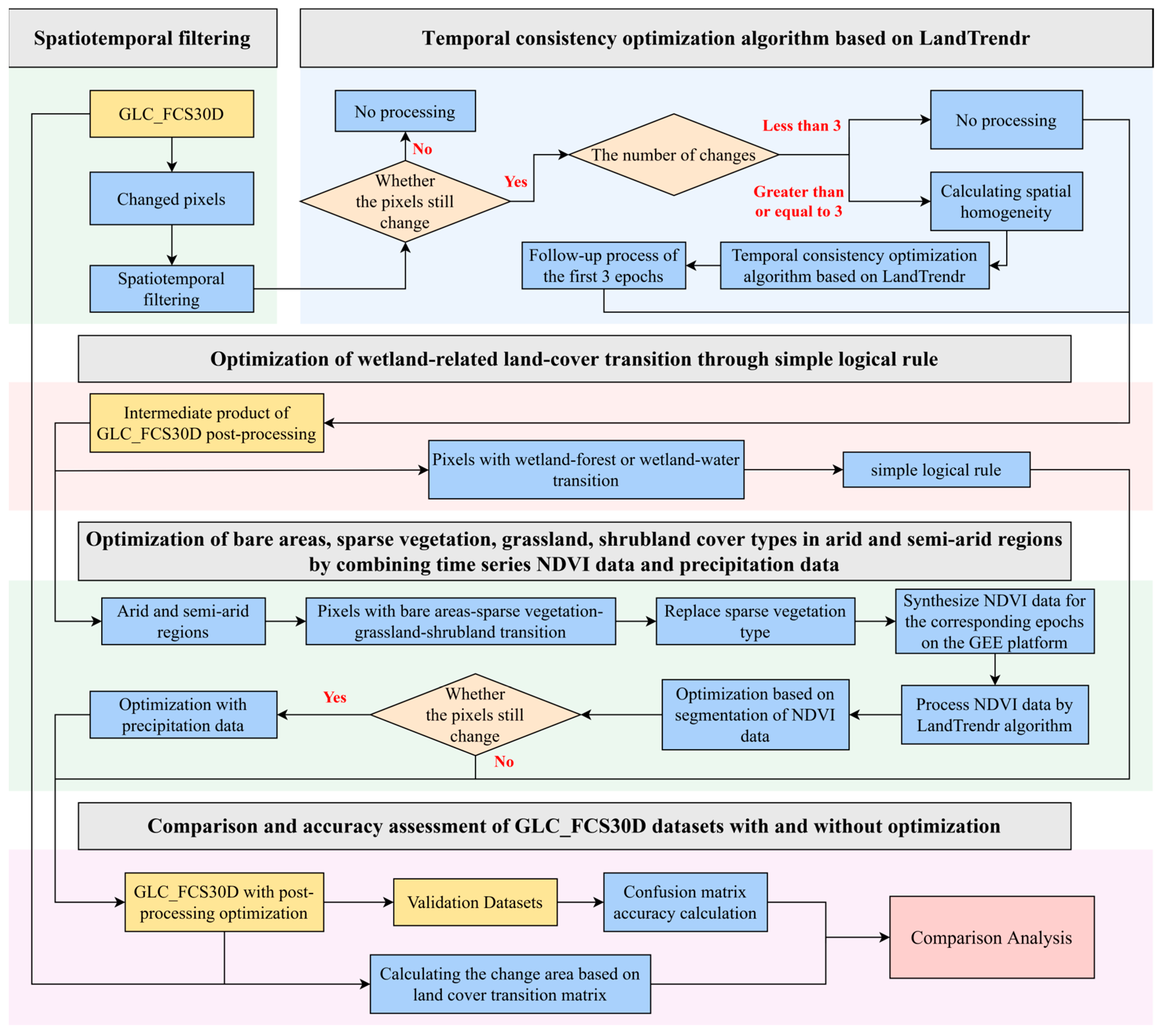
Funding

This research was funded by the National Key Research and Development Program of China, grant number 2023YFB3907403.

Data Availability Statement

The GLC_FCS30D dataset with post-processing optimization is available upon reasonable requests. We will soon release an enhanced version of GLC_FCS30D dataset with an improved classification and post-processing algorithm and update it to 2025.

Conflicts of Interest

The authors declare that they have no known competing financial interests or personal relationships that could have appeared to influence the work reported in this paper. All authors have read and agreed to the published version of the manuscript.

Appendix A

Table A1. The correspondence between fine classification system (35 land cover types) of GLC_FCS30D and basic classification system (10 major land cover types) and LCCS level-1 validation system (17 land cover types).
Fine Classification SystemIDLevel-1 Validation Systems10 Major Land Cover Types
Rainfed cropland10Rainfed croplandRCPCroplandCRP
Herbaceous cover11
Tree or shrub cover (orchard)12
Irrigated cropland20Irrigated croplandICP
Closed evergreen broadleaved forest51Evergreen broadleaved forestEBFForestFST
Open evergreen broadleaved forest52
Closed deciduous broadleaved forest61Deciduous broadleaved forestBDF
Open deciduous broadleaved forest62
Closed evergreen needle-leaved forest71Evergreen needleleaved forestENF
Open evergreen needle-leaved forest72
Closed deciduous needle-leaved forest81Deciduous needleleaved forestDNF
Open deciduous needle-leaved forest82
Closed mixed-leaf forest91Mixed-leaf forestMFT
Open mixed-leaf forest92
Shrubland120ShrublandSHRShrublandSHR
Evergreen shrubland121
Deciduous shrubland122
Grassland130GrasslandGRSGrasslandGRS
Lichens and mosses140Lichens and mossesLMSTundraTUD
Swamp181Inland wetlandIWLWetlandWET
Marsh182
Flooded flat183
Saline184
Mangrove185Coastal wetlandCWL
Salt marsh186
Tidal flat187
Impervious surfaces190Impervious surfacesIMPImpervious surfacesIMP
Sparse vegetation200Sparse vegetationSVGBare areasBAL
Sparse shrubland201
Sparse herbaceous cover202
Bare areas200Bare areasBAL
Consolidated bare areas201
Unconsolidated bare areas202
Water body210Water bodyWTRWater bodyWTR
Permanent ice and snow220Permanent snow and icePSIPermanent snow and icePSI
Table A2. The correspondence between the fine classification system of the GLC_FCS30D product and the 8 land cover classifications of LUCAS.
Fine Classification SystemIDLUCAS Classification SystemLCMAP Classification System
Rainfed cropland10CroplandCRPCroplandCRP
Herbaceous cover cropland11
Tree or shrub cover cropland12
Irrigated cropland20
Closed evergreen broadleaved forest51ForestFSTTree CoverFST
Open evergreen broadleaved forest52
Closed deciduous broadleaved forest61
Open deciduous broadleaved forest62
Closed evergreen needle-leaved forest71
Open evergreen needle-leaved forest72
Closed deciduous needle-leaved forest81
Open deciduous needle-leaved forest82
Closed mixed-leaf forest91
Open mixed-leaf forest92
Shrubland120ShrublandSHRGrass/ShrubGRS/SHR
Evergreen shrubland121
Deciduous shrubland122
Grassland130GrasslandGRS
Lichens and mosses140
Swamp181WetlandWETWetlandWET
Marsh182
Flooded flat183
Saline184
Mangrove185
Salt marsh186
Tidal flat187
Impervious surfaces190Impervious surfacesIMPDevelopedIMP
Sparse vegetation150BarrenBALBarrenBAL
Sparse shrubland152
Sparse herbaceous cover153
Bare areas200
Consolidated bare areas201
Unconsolidated bare areas202
Water body210WaterWTRWaterWTR
Permanent snow and ice220Ice/SnowPSI

References

  1. Tuanmu, M.N.; Jetz, W. A global 1-km consensus land-cover product for biodiversity and ecosystem modelling. Glob. Ecol. Biogeogr. 2014, 23, 1031–1045. [Google Scholar] [CrossRef]
  2. Brown, C.F.; Brumby, S.P.; Guzder-Williams, B.; Birch, T.; Hyde, S.B.; Mazzariello, J.; Czerwinski, W.; Pasquarella, V.J.; Haertel, R.; Ilyushchenko, S. Dynamic world, near real-time global 10 m land use land cover mapping. Sci. Data 2022, 9, 251. [Google Scholar] [CrossRef]
  3. Li, Z.; He, W.; Cheng, M.; Hu, J.; Yang, G.; Zhang, H. SinoLC-1: The first 1-meter resolution national-scale land-cover map of China created with the deep learning framework and open-access data. Earth Syst. Sci. Data Discuss. 2023, 15, 4749–4780. [Google Scholar] [CrossRef]
  4. Zhao, T.; Mu, X.; Song, W.; Liu, Y.; Xie, Y.; Zhong, B.; Xie, D.; Jiang, L.; Yan, G. Mapping spatially seamless fractional vegetation cover over china at a 30-m resolution and semimonthly intervals in 2010–2020 based on google earth engine. J. Remote Sens. 2023, 3, 0101. [Google Scholar] [CrossRef]
  5. Ban, Y.; Gong, P.; Giri, C. Global land cover mapping using earth observation satellite data: Recent progresses and challenges. ISPRS J. Photogramm. Remote Sens. 2015, 103, 1–6. [Google Scholar] [CrossRef]
  6. Wang, J.; Bretz, M.; Dewan, M.A.A.; Delavar, M.A. Machine learning in modelling land-use and land cover-change (lulcc): Current status, challenges and prospects. Sci. Total Environ. 2022, 822, 153559. [Google Scholar] [CrossRef]
  7. Wulder, M.A.; Coops, N.C.; Roy, D.P.; White, J.C.; Hermosilla, T. Land cover 2.0. Int. J. Remote Sens. 2018, 39, 4254–4284. [Google Scholar] [CrossRef]
  8. Zhu, L.; La, Y.; Shi, R.; Peng, S. Removing land cover spurious change by geo-eco zoning rule base. Int. Arch. Photogramm. Remote Sens. Spat. Inf. Sci. 2020, 42, 677–683. [Google Scholar] [CrossRef]
  9. Team, U.; Bontemps, S.; Defourny, P.; Van Bogaert, E.; Team, E.; Arino, O.; Kalogirou, V.; Perez, J.R. Globcover 2009 Products Description and Validation Report; UCLouvain & ESA Team: Brussels, Belgium, 2011. [Google Scholar]
  10. Mi, J.; Liu, L.; Zhang, X.; Chen, X.; Gao, Y.; Xie, S. Impact of geometric misregistration in globeland30 on land-cover change analysis, a case study in China. J. Appl. Remote Sens. 2022, 16, 014516. [Google Scholar] [CrossRef]
  11. Xian, G.Z.; Smith, K.; Wellington, D.; Horton, J.; Zhou, Q.; Li, C.; Auch, R.; Brown, J.F.; Zhu, Z.; Reker, R.R. Implementation of the ccdc algorithm to produce the lcmap collection 1.0 annual land surface change product. Earth Syst. Sci. Data 2022, 14, 143–162. [Google Scholar] [CrossRef]
  12. Xie, S.; Liu, L.; Zhang, X.; Yang, J. Mapping the annual dynamics of land cover in Beijing from 2001 to 2020 using landsat dense time series stack. ISPRS J. Photogramm. Remote Sens. 2022, 185, 201–218. [Google Scholar] [CrossRef]
  13. Zhang, X.; Zhao, T.; Xu, H.; Liu, W.; Wang, J.; Chen, X.; Liu, L. glc_fcs30d: The first global 30 m land-cover dynamics monitoring product with a fine classification system for the period from 1985 to 2022 generated using dense-time-series Landsat imagery and the continuous change-detection method. Earth Syst. Sci. Data 2024, 16, 1353–1381. [Google Scholar] [CrossRef]
  14. Zhu, Z.; Woodcock, C.E. Continuous change detection and classification of land cover using all available landsat data. Remote Sens. Environ. 2014, 144, 152–171. [Google Scholar] [CrossRef]
  15. Friedl, M.A.; Woodcock, C.E.; Olofsson, P.; Zhu, Z.; Loveland, T.; Stanimirova, R.; Arevalo, P.; Bullock, E.; Hu, K.-T.; Zhang, Y.; et al. Medium spatial resolution mapping of global land cover and land cover change across multiple decades from Landsat. Front. Remote Sens. 2022, 3, 894571. [Google Scholar] [CrossRef]
  16. Ding, N.; Li, M. Mapping forest abrupt disturbance events in southeastern China—Comparisons and tradeoffs of landsat time series analysis algorithms. Remote Sens. 2023, 15, 5408. [Google Scholar] [CrossRef]
  17. Li, Z.; Liu, W.; Zhang, X.; Liu, L. Carbon emissions from global impervious surface expansion between 1985 and 2020. Sci. Total Environ. 2024, 952, 175856. [Google Scholar] [CrossRef]
  18. Liu, W.; Zhang, X.; Xu, H.; Zhao, T.; Wang, J.; Li, Z.; Liu, L. Characterizing the accelerated global carbon emissions from forest loss during 1985–2020 using fine-resolution remote sensing datasets. Remote Sens. 2024, 16, 978. [Google Scholar] [CrossRef]
  19. Petitjean, F.; Kurtz, C.; Passat, N.; Gançarski, P. Spatio-temporal reasoning for the classification of satellite image time series. Pattern Recognit. Lett. 2012, 33, 1805–1815. [Google Scholar] [CrossRef]
  20. Clark, M.L.; Aide, T.M.; Grau, H.R.; Riner, G. A scalable approach to mapping annual land cover at 250 m using modis time series data: A case study in the dry chaco ecoregion of south america. Remote Sens. Environ. 2010, 114, 2816–2832. [Google Scholar] [CrossRef]
  21. Kennedy, R.E.; Cohen, W.B.; Schroeder, T.A. Trajectory-based change detection for automated characterization of forest disturbance dynamics. Remote Sens. Environ. 2007, 110, 370–386. [Google Scholar] [CrossRef]
  22. Jin, S.; Yang, L.; Danielson, P.; Homer, C.; Fry, J.; Xian, G. A comprehensive change detection method for updating the national land cover database to circa 2011. Remote Sens. Environ. 2013, 132, 159–175. [Google Scholar] [CrossRef]
  23. Jin, S.; Homer, C.; Yang, L.; Danielson, P.; Dewitz, J.; Li, C.; Zhu, Z.; Xian, G.; Howard, D. Overall methodology design for the United States national land cover database 2016 products. Remote Sens. 2019, 11, 2971. [Google Scholar] [CrossRef]
  24. Liu, D.; Cai, S. A spatial-temporal modeling approach to reconstructing land-cover change trajectories from multi-temporal satellite imagery. Ann. Assoc. Am. Geogr. 2012, 102, 1329–1347. [Google Scholar] [CrossRef]
  25. Cai, S.; Liu, D.; Sulla-Menashe, D.; Friedl, M.A. Enhancing modis land cover product with a spatial–temporal modeling algorithm. Remote Sens. Environ. 2014, 147, 243–255. [Google Scholar] [CrossRef]
  26. Yang, J.; Huang, X. The 30 m annual land cover dataset and its dynamics in China from 1990 to 2019. Earth Syst. Sci. Data 2021, 13, 3907–3925. [Google Scholar] [CrossRef]
  27. Moser, G.; Serpico, S.B.; Benediktsson, J.A. Markov random field models for supervised land cover classification from very high resolution multispectral remote sensing images. In Proceedings of the 2012 Tyrrhenian Workshop on Advances in Radar and Remote Sensing (TyWRRS), Naples, Italy, 12–14 September 2012; IEEE: Piscataway, NJ, USA, 2012; pp. 235–242. [Google Scholar]
  28. Zhang, X.; Liu, L.; Chen, X.; Gao, Y.; Xie, S.; Mi, J. glc_fcs30: Global land-cover product with fine classification system at 30 m using time-series Landsat imagery. Earth Syst. Sci. Data 2021, 13, 2753–2776. [Google Scholar] [CrossRef]
  29. Zhang, X.; Liu, L.; Zhao, T.; Chen, X.; Lin, S.; Wang, J.; Mi, J.; Liu, W. gwl_fcs30: A global 30 m wetland map with a fine classification system using multi-sourced and time-series remote sensing imagery in 2020. Earth Syst. Sci. Data 2023, 15, 265–293. [Google Scholar] [CrossRef]
  30. Zhao, T.; Zhang, X.; Gao, Y.; Mi, J.; Liu, W.; Wang, J.; Jiang, M.; Liu, L. Assessing the accuracy and consistency of six fine-resolution global land cover products using a novel stratified random sampling validation dataset. Remote Sens. 2023, 15, 2285. [Google Scholar] [CrossRef]
  31. Stehman, S.V.; Pengra, B.W.; Horton, J.A.; Wellington, D.F. Validation of the us geological survey’s land change monitoring, assessment and projection (lcmap) collection 1.0 annual land cover products 1985–2017. Remote Sens. Environ. 2021, 265, 112646. [Google Scholar] [CrossRef]
  32. Ballin, M.; Barcaroli, G.; Masselli, M.; Scarnó, M. Redesign Sample for Land use/Cover Area Frame Survey (LUCAS); Publications Office of the European Union: Luxembourg, 2018; Eurostat: Statistical Working Papers. [Google Scholar] [CrossRef]
  33. Zomer, R.J.; Xu, J.; Trabucco, A. Version 3 of the global aridity index and potential evapotranspiration database. Sci. Data 2022, 9, 409. [Google Scholar] [CrossRef]
  34. Williams, D.L.; Goward, S.; Arvidson, T. Landsat. Photogramm. Eng. Remote Sens. 2006, 72, 1171–1178. [Google Scholar] [CrossRef]
  35. Wulder, M.A.; Loveland, T.R.; Roy, D.P.; Crawford, C.J.; Masek, J.G.; Woodcock, C.E.; Allen, R.G.; Anderson, M.C.; Belward, A.S.; Cohen, W.B.; et al. Current status of landsat program, science, and applications. Remote Sens. Environ. 2019, 225, 127–147. [Google Scholar] [CrossRef]
  36. Muñoz-Sabater, J.; Dutra, E.; Agustí-Panareda, A.; Albergel, C.; Arduini, G.; Balsamo, G.; Boussetta, S.; Choulga, M.; Harrigan, S.; Hersbach, H.; et al. Era5-land: A state-of-the-art global reanalysis dataset for land applications. Earth Syst. Sci. Data 2021, 13, 4349–4383. [Google Scholar] [CrossRef]
  37. Li, X.; Gong, P.; Liang, L. A 30-year (1984–2013) record of annual urban dynamics of Beijing City derived from Landsat data. Remote Sens. Environ. 2015, 166, 78–90. [Google Scholar] [CrossRef]
  38. Zhang, X.; Liu, L.Y.; Zhao, T.T.; Gao, Y.; Chen, X.D.; Mi, J. Gisd30: Global 30 m impervious-surface dynamic dataset from 1985 to 2020 using time-series landsat imagery on the google earth engine platform. Earth Syst. Sci. Data 2022, 14, 1831–1856. [Google Scholar] [CrossRef]
  39. Kenny, Q.Y. Indicator function and its application in two-level factorial designs. Ann. Stat. 2003, 31, 984–994. [Google Scholar]
  40. Zhang, X.; Liu, L.; Zhang, W.; Guan, L.; Bai, M.; Zhao, T.; Li, Z.; Chen, X. Tracking gain and loss of impervious surfaces by integrating continuous change detection and multitemporal classifications from 1985 to 2022 in Beijing. Int. J. Appl. Earth Obs. Geoinf. 2024, 135, 104268. [Google Scholar] [CrossRef]
  41. Kennedy, R.E.; Yang, Z.; Cohen, W.B. Detecting trends in forest disturbance and recovery using yearly landsat time series: 1. Landtrendr—Temporal segmentation algorithms. Remote Sens. Environ. 2010, 114, 2897–2910. [Google Scholar] [CrossRef]
  42. Pasquarella, V.J.; Arévalo, P.; Bratley, K.H.; Bullock, E.L.; Gorelick, N.; Yang, Z.; Kennedy, R.E. Demystifying landtrendr and ccdc temporal segmentation. Int. J. Appl. Earth Obs. Geoinf. 2022, 110, 102806. [Google Scholar] [CrossRef]
  43. Pekel, J.-F.; Cottam, A.; Gorelick, N.; Belward, A.S. High-resolution mapping of global surface water and its long-term changes. Nature 2016, 540, 418–422. [Google Scholar] [CrossRef]
  44. Huete, A.R.; Liu, H.Q. An error and sensitivity analysis of the atmospheric-and soil-correcting variants of the ndvi for the modis-eos. IEEE Trans. Geosci. Remote Sens. 1994, 32, 897–905. [Google Scholar] [CrossRef]
  45. Leprieur, C.; Kerr, Y.; Mastorchio, S.; Meunier, J. Monitoring vegetation cover across semi-arid regions: Comparison of remote observations from various scales. Int. J. Remote Sens. 2000, 21, 281–300. [Google Scholar] [CrossRef]
  46. Jiang, Z.; Huete, A.R.; Chen, J.; Chen, Y.; Li, J.; Yan, G.; Zhang, X. Analysis of ndvi and scaled difference vegetation index retrievals of vegetation fraction. Remote Sens. Environ. 2006, 101, 366–378. [Google Scholar] [CrossRef]
  47. Wang, Z.; Bastin, G.N.; Liu, L.; Caccetta, P.A.; Peng, D. Estimating woody above-ground biomass in an arid zone of central Australia using landsat imagery. J. Appl. Remote Sens. 2015, 9, 096036. [Google Scholar] [CrossRef]
  48. White, J.C.; Wulder, M.; Hobart, G.; Luther, J.; Hermosilla, T.; Griffiths, P.; Coops, N.; Hall, R.; Hostert, P.; Dyk, A.; et al. Pixel-based image compositing for large-area dense time series applications and science. Can. J. Remote Sens. 2014, 40, 192–212. [Google Scholar] [CrossRef]
  49. Song, C.; Woodcock, C.E.; Seto, K.C.; Lenney, M.P.; Macomber, S.A. Classification and change detection using landsat tm data: When and how to correct atmospheric effects? Remote Sens. Environ. 2001, 75, 230–244. [Google Scholar] [CrossRef]
  50. Schmidt, K.; Skidmore, A. Spectral discrimination of vegetation types in a coastal wetland. Remote Sens. Environ. 2003, 85, 92–108. [Google Scholar] [CrossRef]
  51. Foody, G.M. Status of land cover classification accuracy assessment. Remote Sens. Environ. 2002, 80, 185–201. [Google Scholar] [CrossRef]
  52. Olofsson, P.; Foody, G.M.; Herold, M.; Stehman, S.V.; Woodcock, C.E.; Wulder, M.A. Good practices for estimating area and assessing accuracy of land change. Remote Sens. Environ. 2014, 148, 42–57. [Google Scholar] [CrossRef]
  53. Hu, Y.; Batunacun; Zhen, L.; Zhuang, D. Assessment of land-use and land-cover change in Guangxi, China. Sci. Rep. 2019, 9, 2189. [Google Scholar] [CrossRef]
  54. Bagwan, W.A.; Sopan Gavali, R. Dam-triggered land use land cover change detection and comparison (transition matrix method) of urmodi river watershed of maharashtra, India: A remote sensing and gis approach. Geol. Ecol. Landsc. 2023, 7, 189–197. [Google Scholar] [CrossRef]
  55. Bastos, A.; Ciais, P.; Sitch, S.; Aragao, L.; Chevallier, F.; Fawcett, D.; Rosan, T.M.; Saunois, M.; Gunther, D.; Perugini, L.; et al. On the use of earth observation to support estimates of national greenhouse gas emissions and sinks for the global stocktake process: Lessons learned from esa-cci reccap2 comment. Carbon Balance Manag. 2022, 17, 15. [Google Scholar] [CrossRef] [PubMed]
  56. Liu, B.; Chen, J.; Chen, J.; Zhang, W. Land cover change detection using multiple shape parameters of spectral and ndvi curves. Remote Sens. 2018, 10, 1251. [Google Scholar] [CrossRef]
  57. Zhu, L.; Gao, D.; Jia, T.; Zhang, J. Using eco-geographical zoning data and crowdsourcing to improve the detection of spurious land cover changes. Remote Sens. 2021, 13, 3244. [Google Scholar] [CrossRef]
Figure 1. Workflow of post-processing optimization of GLC_FCS30D.
Remotesensing 17 01558 g001
Figure 2. Example of using the LandTrendr algorithm to segment the homogeneity of the time series.
Remotesensing 17 01558 g002
Figure 3. Optimization of bare areas, sparse vegetation, grassland, and shrubland cover types in arid and semi-arid regions by combining time-series NDVI data and precipitation data.
Remotesensing 17 01558 g003
Figure 4. NDVI composite and segmentation example: (a) NDVI of the E140S15 block in 2000; (b) NDVI of the E140S15 block in 2020; (c) segmentation results of NDVI for the E140S15 block over 26 epochs; (d) NDVI of the E35N5 block in 2000; (e) NDVI of the E35N5 block in 2020; (f) segmentation results of NDVI for the E35N5 block over 26 epochs.
Remotesensing 17 01558 g004
Figure 5. Comparison of forest and cropland area changes in GLC_FCS30D products with and without post-processing optimization: Comparison of (a) forest loss area, (b) cropland loss area, (c) forest gain area, (d) and cropland gain area.
Remotesensing 17 01558 g005
Figure 6. Land cover change intensity of wetland–water bodies and wetland–forests at a resolution of 0.05 degrees: GLC_FCS30D product (a) without and (b) with post-processing optimization; (cf) zoomed-in view of local areas.
Remotesensing 17 01558 g006
Figure 7. Land cover change intensity of bare areas–sparse vegetation–grassland–shrubland in arid and semi-arid regions at a resolution of 0.05 degrees: GLC_FCS30D product (a) without and (b) with post-processing optimization; (cf) zoomed-in view of local areas.
Remotesensing 17 01558 g007
Figure 8. Distribution map of land cover changes in the GLC_FCS30D product from 1985 to 2022: (a) without and (b) with post-processing optimization.
Remotesensing 17 01558 g008
Figure 9. Comparison of details of specific regions of the GLC_FCS30D products with and without post-processing optimization: (a) a region in South America; (b) a region in Asia.
Remotesensing 17 01558 g009
Figure 10. Comparison of details of specific regions of the GLC_FCS30D products with and without post-processing optimization: (a) another region in South America; (b) another region in Asia.
Remotesensing 17 01558 g010
Figure 11. Cumulative net change area of 10 major land cover types in GLC_FCS30D products with and without post-processing optimization: (a) cropland, (b) forest, (c) shrubland, (d) grassland, (e) tundra, (f) wetland, (g) impervious surfaces, (h) bare areas, (i) water body, and (j) permanent snow and ice.
Remotesensing 17 01558 g011
Figure 12. Time series of the O.A. of the GLC_FCS30D product with post-processing optimization using the LCMAP_Val annual reference dataset for the contiguous United States (CONUS) from 1985 to 2021.
Remotesensing 17 01558 g012
Figure 13. Overall accuracy (O.A.) of the GLC_FCS30D product with post-processing optimization for the European Union (EU) region using the LUCAS validation dataset from 2006 to 2018.
Remotesensing 17 01558 g013
Figure 14. Producer’s accuracy (P.A.) and user’s accuracy (U.A.) of the GLC_FCS30D product with post-processing optimization for the European Union (EU) region using the LUCAS validation dataset from 2006 to 2018.
Remotesensing 17 01558 g014
Figure 15. Comparison of GLC_FCS30D product with post-processing optimization and LCMAP product in the contiguous United States.
Remotesensing 17 01558 g015
Table 1. Transition matrix of 10 major land cover types of GLC_FCS30D product without post-processing optimization (units: Mha).
CRPFSTSHRGRSTUDWETIMPBALWTRPSITotal
CRP0.00311.58187.25249.801.0270.03160.22106.4910.720.121097.23
FST414.630.00427.48176.374.59634.7233.5784.1315.621.091792.19
SHR213.58353.510.00231.293.4977.9520.11131.934.260.961037.08
GRS261.30153.55232.110.002.2845.3925.15204.224.749.41938.15
TUD0.923.133.791.660.007.920.368.251.931.4129.38
WET63.04608.3275.5341.277.310.004.03119.75321.180.331240.76
IMP117.8527.3615.2819.660.313.500.0018.841.380.24204.41
BAL111.0365.58144.38202.639.37130.8724.990.0024.1233.22746.19
WTR8.3613.094.364.912.03325.392.1531.550.0012.23404.06
PSI0.110.800.838.800.950.280.2224.8510.700.0047.55
Total1190.811536.911091.02936.4131.351296.04270.79730.00394.6459.027537.00
Table 2. Transition matrix of 10 major land cover types of GLC_FCS30D product with post-processing optimization (units: Mha).
CRPFSTSHRGRSTUDWETIMPBALWTRPSITotal
CRP0.00 129.33 70.54 62.43 0.09 28.28 63.94 39.98 5.63 0.04 400.27
FST231.79 0.00 192.50 90.49 2.48 40.67 14.84 34.22 8.12 0.38 615.48
SHR95.49 120.29 0.00 36.58 0.83 27.30 6.96 11.43 1.39 0.28 300.57
GRS78.23 60.60 36.43 0.00 0.71 16.93 8.97 10.18 1.92 2.46 216.42
TUD0.07 1.21 0.99 0.41 0.00 2.48 0.09 3.77 0.62 0.55 10.18
WET20.74 13.64 23.61 12.55 1.96 0.00 2.00 37.14 27.26 0.28 139.18
IMP25.40 6.67 2.81 4.01 0.04 1.76 0.00 4.66 0.57 0.07 45.98
BAL48.78 16.78 12.07 11.12 4.13 50.36 9.95 0.00 8.60 11.44 173.24
WTR3.29 4.66 1.32 2.14 0.65 38.91 1.32 15.40 0.00 3.47 71.17
PSI0.02 0.11 0.18 1.60 0.16 0.25 0.05 4.16 1.99 0.00 8.52
Total503.80 353.29 340.45 221.33 11.04 206.94 108.12 160.96 56.10 18.97 1981.00
Table 3. Cumulative net change area of the GLC_FCS30D products with and without post-processing optimization from 1985 to 2022 (units: Mha).
Land Cover TypeGLC_FCS30D without Post-Processing OptimizationGLC_FCS30D with Post-Processing Optimization
Cropland93.58103.53
Forest−255.27−266.19
Shrubland53.9439.89
Grassland−1.731.90
Tundra1.980.86
Wetland55.2967.76
Impervious surfaces66.3869.14
Bare areas−16.20−15.27
Water body−9.43−12.07
Permanent snow and ice11.4710.45
Table 4. Error matrix of the 2020 GLC_FCS30D product with post-processing optimization based on the basic classification system.
MapO.A. = 81.15% (±0.26%)
ReferenceCRPFSTGRSSHRWETWTRTUDIMPBALPSITotalP.A.SE
CRP13,674381426223661608154014,92191.640.44
FST49824,4393716252103135978226,31692.860.31
GRS1084103249697862141379479677919854.081.02
SHR554158078542951561315454642790954.701.10
WET77423132145361633028181863495872.971.24
WTR4266174025425191212255299284.091.31
TUD410512412122292078244016294170.661.65
IMP8447133281024252260447495.040.64
BAL105327114965129471387816107985679.390.80
PSI231913035210401165129889.751.65
Total16,12428,10875676776459730252709455410,0961307
U.A.84.8186.9565.9563.5478.5783.2676.7193.3777.5689.14
SE0.550.391.071.141.191.331.590.720.811.69
Note: The producer’s accuracy (P.A.) and user’s accuracy (U.A.) values in the table are accompanied by their respective standard errors (SE), all expressed as percentages (%). The corresponding abbreviations for the 10 categories of the basic classification system are provided in Table A1.
Table 5. Error matrix of the 2020 GLC_FCS30D product with post-processing optimization based on the LCCS level-1 validation system.
MapO.A. = 74.24% (±0.29%)
ReferenceRCPICPEBFDBFENFDNFMFTSHRGRSLMSSVGIWLCWLIMPBALWTRPSITotalP.A.SE
RCP11,665361361824571121640203634328131012,81591.030.49
ICP33116420000072405236530150210677.971.77
EBF19332772594623293382591050500312160967779.810.80
DBF2051461255105213223020717431082122102771671.411.01
ENF4021872434786204109344030961610110576383.030.97
DNF9021121041674558450142100630205381.531.68
MFT30301381271246648300900010110759.952.89
SHR521332947553151259142957851540515154559132790954.701.10
GRS10087615353517914421786496979783209547184137919854.081.02
LMS221203843312112420783542022862916294170.661.65
SVG528668413163962922261108586421368260.461.58
IWL56151047617653213612728143223219812282763366560.931.58
CWL427122095010126106065540129381.852.10
IMP721216141322321321271425214100447495.040.64
BAL369232001803154424923823045122586617473.081.11
WTR2220191030614017128150104121725195299284.091.31
PSI11012001319212100019351165129889.751.65
Total14,220190492948552658028038796776756727094554320913884554554230251307
U.A.82.0386.2483.1264.4372.7659.7175.5163.5565.8676.7149.0569.4576.2093.3781.4183.2689.14
SE0.631.550.761.011.081.822.841.141.071.591.451.592.240.721.021.331.69
Note: The producer’s accuracy (P.A.) and user’s accuracy (U.A.) values in the table are accompanied by their respective standard errors (SE), all expressed as percentages. The corresponding abbreviations for the 17 categories of the LCCS level-1 validation system are provided in Table A1.
Table 6. The error matrix of changed and unchanged pixels in GLC_FCS30D with post-processing optimization, as evaluated using the LCMAP_Val and LUCAS validation datasets.
LCMAP_Val UnchangedChangedTotalP.A. (SE)
Unchanged22,406150423,91093.71 (0.30)
Changed7842306309074.63 (1.53)
Total23,190381027,000
U.A. (SE)96.62 (0.23)60.52 (1.55)
O.A. (SE)91.53 (0.33)
LUCAS UnchangedChangedTotalP.A. (SE)
Unchanged906,50725,963932,47097.22 (0.03)
Changed68,94089,453158,39356.48 (0.24)
Total975,447115,4161,090,863
U.A. (SE)92.93 (0.05)77.50 (0.24)
O.A. (SE)91.16 (0.05)
Table 7. Cumulative land cover transition matrix for the contiguous United States (CONUS) region for the GLC_FCS30D product with and without post-processing optimization and the LCMAP annual land cover product (units: Mha).
IMPCRPGRS/SHRFSTWTRWETPSIBALTotal
GLC_FCS30D without post-processing optimizationIMP0.006.086.387.370.110.260.000.6920.89
CRP10.050.0067.1123.290.686.360.002.06109.55
GRS/SHR8.2163.740.0037.800.323.140.018.18121.41
FST8.2428.3541.340.000.9961.560.017.75148.24
WTR0.130.370.270.910.007.450.021.2210.37
WET0.305.983.1060.647.550.000.006.8484.41
PSI0.000.000.010.010.020.000.000.030.06
BAL0.841.647.506.381.206.750.050.0024.36
Total27.78106.16125.69136.3910.8785.520.0926.79519.29
GLC_FCS30D with post-processing optimizationIMP0.001.031.341.900.050.140.000.154.62
CRP3.890.0026.048.250.442.120.000.5541.29
GRS/SHR3.0925.190.0012.800.181.210.003.6246.09
FST3.1311.5416.100.000.3916.880.001.6949.73
WTR0.080.140.110.240.003.830.010.294.70
WET0.161.430.9714.723.460.000.000.7021.44
PSI0.000.000.000.000.000.000.000.010.01
BAL0.280.373.270.770.290.730.020.005.73
Total10.6339.7047.8338.684.8124.920.046.99173.60
LCMAP product (CONUS region)IMP0.003.014.620.830.220.050.000.439.15
CRP4.320.0025.462.861.010.590.000.6734.91
GRS/SHR4.6423.320.0047.971.440.630.002.9380.94
FST1.864.3950.340.000.330.170.001.2558.33
WTR0.200.711.300.240.000.660.000.853.97
WET0.130.540.730.160.640.000.000.102.31
PSI0.000.000.000.000.000.000.000.000.00
BAL0.570.603.390.200.560.100.000.005.42
Total11.7332.5885.8552.254.212.190.006.23195.03
Disclaimer/Publisher’s Note: The statements, opinions and data contained in all publications are solely those of the individual author(s) and contributor(s) and not of MDPI and/or the editor(s). MDPI and/or the editor(s) disclaim responsibility for any injury to people or property resulting from any ideas, methods, instructions or products referred to in the content.

