Hybrid Filtering Technique for Accurate GNSS State Estimation

Abstract

The Global Navigation Satellite System (GNSS) is extensively utilized in various applications that require triangulation solutions for positioning, navigation, and timing (PNT). These solutions are obtained by solving state estimates, traditionally using methods like weighted least squares (WLS) and Kalman Filters (KF). While these conventional approaches are foundational, they frequently encounter challenges related to robustness, particularly the necessity for precise noise statistics and the reliance on potentially accurate prior assumptions. This paper introduces a hybrid approach to GNSS state estimation, which integrates deep neural networks (DNNs) with the KF framework, employing the maximum likelihood principle for unsupervised training. Our methodology combines the strengths of DNNs with conventional KF techniques, leveraging established model-based priors while enabling flexible, data-driven modifications. We parameterize components of the Extended Kalman Filter (EKF) using neural networks, training them with a probabilistically informed maximum likelihood loss function and backpropagation. We demonstrate that this hybrid method outperforms classical algorithms both in terms of accuracy and flexibility for easier implementation, showing better than 30% improvement in the variance of the horizontal position for the simulated as well as the real-world dynamic receiver dataset. For the real-world dynamic dataset, our method also provides a better fit to the measurements than the classical algorithms.

1. Introduction

Geodesy relies on precise positioning technologies for accurate and continuous monitoring of spatial coordinates on a global scale [1]. One of the most transformative tools in modern geodesy and geomapping is the Global Navigation Satellite System (GNSS), which enables accurate spatial measurements critical for applications such as land surveying, tectonic studies, and real-time navigation [2]. The increasing demand for sub-centimeter accuracy has driven advancements in GNSS-based positioning techniques, including real-time kinematic (RTK) positioning and precise point positioning (PPP), which refine geospatial data accuracy for scientific and commercial applications [3].

GNSS is a critical technology for positioning, velocity, and timing. However, its accuracy can be compromised by various sources of errors such as ionospheric and tropospheric delays, satellite clock inaccuracies, as well as signal interferences such as multipath errors, jamming, and spoofing [3,4]. Triangulation or trilateration is a fundamental aspect of GNSS navigation that involves solving a set of nonlinear observation equations to estimate the receiver’s state [5]. Conventionally, this is achieved by employing the techniques of weighted least squares (WLS) and nonlinear Kalman Filters (KF) such as the Extended Kalman Filter (EKF) [6] and the Unscented Kalman Filter (UKF) [7]. However, in practical scenarios, these methods are known to encounter issues with initialization, robustness, and mismatched priors [8]. Although conventional post-processing techniques have effectively reduced these problems, their real-time application is often limited and expensive [9]. As a result of these challenges, there is a growing need for practical and data-driven models to improve the quality and reliability of navigation solutions. We note that methods such as factor graph optimization [10] have been implemented instead of the classical Kalman filter and have proven to be more robust.

Significant efforts have been made in applying deep neural networks (DNNs) for GNSS [11]. In permutation invariant DNNs, set transformers were employed for triangulation, with the line-of-sight vectors and pseudorange residuals as inputs to iteratively provide position correction, which demonstrated approximately 30% performance improvement to the WLS method on a real dataset [12]. Additionally, Liu et al. employed encoder–decoder architectures for position correction within urban settings, utilizing the distribution of environmental factors, such as building heights and road distribution, to compensate for positioning errors [13]. Similarly, Zhang et al. and Hochreiter et al. utilized a long short-term memory (LSTM) network to predict pseudorange errors arising from multipath and non-line-of-sight reception [14,15]. However, these works excluded model-based priors, relying solely on neural networks for function approximation to improve estimation. However, a hybrid approach combining neural networks and a model-based KF has recently emerged. For example, Mohanty and Gao introduced a hybrid graph-convolution neural network (GCNN) fused with a KF, which is designed for triangulation, thus demonstrating further improvements compared to baseline methods like WLS, the set transformer approach, and KFs on real-world datasets [16]. However, these methods do not fully explore the potential of extending the estimation algorithm in a more structured manner. This approach addresses mismodeling issues in the independent components of the estimation process, including in the observation and dynamics models, without relying solely on the input–output mappings, which are commonly used in classical deep learning methods and often fail to capture the underlying physics or dynamics of the system. To this end, recent advances have led to innovative extensions of probabilistic filtering algorithms, which can be learned in end-to-end training, as seen in differentiable filters [17,18]. Alternatively, algorithms utilizing the features of Extended Kalman Filters (EKF) have been developed [19,20,21]. These data-driven models utilize learning algorithms to infer the system response in addition to physics-based models, which rely on first principles.

Building on recent progress in differentiable filtering, our work introduces a differentiable version of the EKF algorithm for navigation applications, which supports end-to-end learning. In contrast to [21], which employs a double update filtering technique, our algorithm utilizes unsupervised learning of the noise parameters to train the neural networks for an Extended Kalman Filter (EKF). This makes our approach more versatile for environments with unknown noise types. The parameters of the proposed framework are optimized using a probabilistically informed loss function derived from the maximum likelihood approach for state-space models [22]. Importantly, this method maintains the probabilistic foundation of the EKF while integrating a parametric representation, thus ensuring a more structured and interpretable architecture compared to conventional unstructured neural network approaches. Additionally, the framework can be trained without relying on the knowledge of the true system states during training, thereby effectively addressing a standard limitation in practical applications, where the actual state of a tracked object is often unavailable without extensive post-processing. The key features of our method are detailed as follows:

• An end-to-end differentiable architecture to improve model-based priors and noise statistics within GNSS state estimation algorithms.
• A gradient descent optimizer demonstration to learn noise statistics automatically, thereby eliminating the need for manual tuning.
• An unsupervised training method based on the maximum likelihood approach that extends the EKF by preserving its probabilistic interpretability, thus ensuring convergence.
• Efficient and simpler implementation and flexibility compared to both the UKF and EKF.

For comparison, we have also implemented other competitive filters along with the DEKF, namely the UKF [7], the EKF [6], the AEKF [23], and WLS [24]. The paper is structured as follows: Section 2 introduces the background and motivation for our method. Section 3 details the design and implementation of differentiable filter architecture and the loss function, along with the training algorithm. Section 4.1 demonstrates the performance of the algorithm in the case of a simulated receiver. The experimental setup and numerical analysis for the real-world scenarios are presented in Section 4.2, while validation and evaluation are covered in Section 4.2.3 and Section 4.2.4. Section 6 concludes the paper.

2. Background and Motivation

2.1. GNSS Model Overview

The pseudorange in most receivers is measured using the TOT (time of transmission) encoded in the signal and TOA (time of arrival) measured by the receiver with the assumption of constant speed of travel of the signal from the satellites to the receiver. Pseudorange for the jth satellite measurement is given by the following:

$${\rho }_j=c(TO{A}_j-TO{T}_j)$$

(1)

Numerous error terms arise from these assumptions, most of which are derived using empirical models and combinations of ranges or are estimated simultaneously with other variables such as process and measurement noise [25]. Consequently, the general form of a triangulation problem is reduced to the following equation:

$${\rho }_j=\parallel \mathbf{r}-{\mathbf{r}}_j\parallel +c\delta t_j+{ϵ}_j$$

(2)

where ${ϵ}_j$ represents the unmodeled errors such as the multipath errors. This implies the state vector in the triangulation problem given by the following:

$$\overrightarrow{\mathbf{x}}=\left[\begin{array}{cccccccc}x& \dot{x}& y& \dot{y}& z& \dot{z}& cdt& \dot{cdt}\end{array}\right]$$

(3)

where x, y, and z are the positional coordinates, $\dot{x}$, $\dot{y}$, and $\dot{z}$ are their respective velocities, $c·dt$ is the receiver clock bias, $\dot{c}·dt$ is the receiver clock drift. Solving the nonlinear Equation (2) for the state vector (3) reduces to the classical problem of state estimation in a nonlinear dynamical system, using which the PVT solutions are obtained [26].

2.2. Discrete Time Extended Kalman Filter

Consider a discrete-time stochastic state-space model governed by differentiable functions f and h, which describe the state dynamics and the observation process, respectively, and can be written as follows:

$$X_{t+1}=f(X_t,u_t)+W_t$$

(4)

$$Y_t=h\left(X_t\right)+V_t$$

(5)

Here, $X_t$ represents the random variable for the state of the system at time t, $Y_t$ is the random variable representing measurement at time t, $u_t$ denotes the control input, and $W_t$ and $V_t$ are zero mean white Gaussian processes characterized by the following covariance structure:

$$\mathbb{E}\left[W_t{W}_s^{\mathrm{T}}\right]=Q_t{\delta }_{ts}$$

(6)

$$\mathbb{E}\left[V_t{V}_s^{\mathrm{T}}\right]=R_t{\delta }_{ts}$$

(7)

where ${\delta }_{ts}$ is the Kronecker delta function. The EKF is a recursive estimation algorithm that estimates the posterior distribution of the state by integrating sequential measurements via Bayes’ rule [27,28]. It operates through a predict–update loop, where it predicts the state and its covariance at the current time step based on previous estimates and then updates them using the current measurement. In the prediction step, the EKF propagates the moments one timestep forward using the following equations:

$$x_{t|t-1}=f(x_{t-1|t-1},u_t)$$

(8)

$$P_{t|t-1}=F_{t-1}{P}_{t-1|t-1}{F}_{t-1}^T+Q_t$$

(9)

where $F_t={\displaystyle \frac{\partial f}{\partial x}}(x_{t-1},u_t)$ is the Jacobian matrix of f with respect to $x_{t-1}$, and $Q_t$ is the noise covariance matrix of the process. In the update step, the EKF calculates the Kalman gain $K_t$ and updates the state estimate and the covariance matrix using the current measurement as follows:

$$K_t=P_{t|t-1}{H}_t^T{(H_t{P}_{t|t-1}{H}_t^T+R_t)}^{-1}$$

(10)

$$x_t=x_{t|t-1}+K_t(y_t-h\left(x_{t|t-1}\right))$$

(11)

$$P_t=(I-K_t{H}_t)P_{t|t-1}$$

(12)

where $H_t={\displaystyle \frac{\partial h}{\partial x}}\left(x_{t|t-1}\right)$ is the Jacobian matrix of h with respect to x, $R_t$ is the measurement noise covariance matrix, and I is the identity matrix. Unlike least-squared methods such as weighted least squares (WLS), this method accounts for the temporal evolution and prior knowledge of the state. The flow chart for the EKF algorithm is described in detail in the Figure 1. Moreover, by processing measurements sequentially, it enables real-time state estimation while maintaining computational complexity, making this approach particularly effective for nonlinear problems.

Furthermore, the Rauch–Tung–Striebel smoothing method is used to infer posterior distributions based on the whole sequence of available observations [19]. The smoothing process fully utilizes the available data when computing the posterior distributions and generates more accurate inference results instead of only utilizing information before each time step, contrary to the Kalman filtering process.

2.3. Hybrid Model for Accurate GNSS

Designing a simpler EKF filter for estimating the states in (3), we assume constant velocity dynamics for the receiver and clock bias. Hence, the state is represented as follows:

$$x={\left[\begin{array}{cccccccc}x& \dot{x}& y& \dot{y}& z& \dot{z}& cdt& \dot{c}dt\end{array}\right]}^T$$

(13)

where the state transition function (4) is modeled as a moving receiver with linear clock dynamics, which can be written as a matrix, $\mathbf{F}$:

$$\mathbf{F}=\left[\begin{array}{cccccccc}1& \Delta t& 0& 0& 0& 0& 0& 0\\ 0& 1& 0& 0& 0& 0& 0& 0\\ 0& 0& 1& \Delta t& 0& 0& 0& 0\\ 0& 0& 0& 1& 0& 0& 0& 0\\ 0& 0& 0& 0& 1& \Delta t& 0& 0\\ 0& 0& 0& 0& 0& 1& 0& 0\\ 0& 0& 0& 0& 0& 0& 1& \Delta t\\ 0& 0& 0& 0& 0& 0& 0& 1\end{array}\right].$$

(14)

Under the assumption of no hidden parameters ${ϵ}_j$, the general observation model in (2) simplifies to the following:

$${\rho }_j=\parallel \mathbf{r}-{\mathbf{r}}_j\parallel +c\delta t_j.$$

(15)

This equation represents the measurement function in (4). The nonlinear nature of this observation model in triangulation necessitates the use of the EKF instead of the KF.

In this work, the baseline model is presented, with the potential for straightforward extension and design modifications as necessary based on the application under question. Furthermore, additional complexities in transition and observation models for GNSS applications can be explored, allowing for the estimation of additional error parameters through the filter or through the integration of new measurements into the system.

3. Materials and Methods

3.1. Differentiable Kalman Filter

In the practical applications of GNSS state estimation, the EKF often does not understand the underlying system dynamics or noise characteristics. This means there is a need to parameterize part of the estimation algorithm, including the noise covariance or the transition functions. The noise covariance and dynamics models can be fully parametrized for generality by arbitrary classes of suitable functions. The parametrized transition dynamics are given by the following:

$$X_{t+1}=f_{\theta }(X_t,{\mathbf{u}}_t)+W_t$$

(16)

$$Y_t=h_{\varphi }\left(X_t\right)+V_t$$

(17)

where $\{\theta ,\varphi \}$ are unknown parameters to estimate. For any white Gaussian process $W\left(t\right)$, we have the following decomposition:

$$W\left(t\right)={\mu }_t+L_{t}V\left(t\right)$$

(18)

where ${\mu }_t$ is the mean vector (=0, for a Gaussian process), $L_t$ is the Cholesky decomposition of the covariance matrix, and $V\left(t\right)$ is a standard white Gaussian process with identity covariance. The covariance of the process is given by the following:

$$\begin{array}{cc}\hfill \mathbb{E}\left[W_t{W}_s^{\mathrm{T}}\right]& =\mathbb{E}\left[L_{t}V\left(t\right)V{\left(s\right)}^{\mathrm{T}}{L}_s^{\mathrm{T}}\right]\hfill \\ \hfill & =L_t\mathbb{E}\left[V\left(t\right)V{\left(t\right)}^{\mathrm{T}}\right]L_s^{\mathrm{T}}\hfill \\ \hfill & =L_t{L}_s^{\mathrm{T}}{\delta }_{ts},\hfill \end{array}$$

(19)

Thus, by parameterizing a time-dependent triangular matrix and a mean vector, it is possible to fully characterize the noise structure. For process and measurement noises with non-zero mean, without loss of generality, the mean value can be incorporated into the parameterizations of $f_{\theta }$ and $h_{\varphi }$ in (16) and (17). Consequently, only the lower triangular matrices associated with the noise need to be parameterized. Furthermore, it is essential to ensure that these matrices maintain positive diagonal elements at all times. The noise covariance is thus given by the following:

$$Q=K{\left(t\right)}_{\alpha }K{\left(t\right)}_{\alpha }^T$$

(20)

$$R=L{\left(t\right)}_{\beta }L{\left(t\right)}_{\beta }^T$$

(21)

where $K{\left(t\right)}_{\alpha }$ and $L{\left(t\right)}_{\beta }$ are the associated lower triangular matrices, each constrained to have positive diagonal elements. The overall composition influence of all parameters can be given by the vector, $\Phi =\{\alpha ,\beta ,\theta ,\varphi \}$, which is to be learned based on the observations. This allows for the modeling of complex non-stationary system dynamics and error processes. Generally, these matrices are considered to be time-independent, similar to the classical Kalman filtering approach.

3.2. The Loss Function

Traditionally, hyperparameter optimization is performed by maximizing the likelihood function of the observed data, which often uses the expectation-maximization (EM) algorithm, as outlined by Shumway and Stoffer [22], for the classical KF. The EM algorithm iteratively alternates between the expectation step (E-step) and the maximization step (M-step) to update the parameters and improve the likelihood. However, this approach requires expressing the underlying equations in a functional closed-form representation to carry out the M-steps. Alternatively, the Newton–Raphson method can be employed directly, but it becomes computationally expensive for high-dimensional parameters of DNNs due to the cost of computing the Hessian matrix. Recent advances in deep learning, including automatic differentiation [29] and nonlinear optimization techniques [30], provide a powerful alternative to replace the maximization step with a gradient-descent-based approach.

The goal is to maximize the marginal likelihood of the data, which is similar to the classical EM algorithm. However, since this optimization problem is typically divergent, an alternative approach based on the EM algorithm is employed [31]. In this method, the expected joint likelihood is indirectly maximized rather than directly maximizing the marginal likelihood function, given as follows:

$$U\left(\theta \right|{\theta }_{old})=\mathbb{E}\left(\mathcal{L}(X_t=x_1,x_2,\cdots ;Y_t=y_1,y_2,\cdots )\mathbb{P}\left(X_t\right|Y_t,{\theta }_{old})\right)$$

(22)

where the expectation is taken over the previous posterior distribution $(X_{t|T},P_{t|T})$, which is obtained by a smoothing algorithm as shown by Rauch et al., that we name as the RTS smoothing algorithm [32]. Now, the joint likelihood shown above can be factored (see [22]) by utilizing the Markovian property of the Kalman filter:

$$\begin{array}{cc}\hfill \mathcal{L}(X_t=x_1,x_2,\cdots ;Y_t=y_1,y_2,\cdots )& =\mathbb{P}(X_t=x_t|Y_t=y_t)\hfill \\ \hfill & =\mathbb{P}\left(X_0\right)\prod _{t=1}^n\mathbb{P}(X_t=x_t|x_{t-1})\prod _{t=1}^n\mathbb{P}(Y_t=y_t|X_t=x_t)\hfill \end{array}$$

(23)

Using (16) and (17), we obtain the following conditional distributions of the state and measurements

$$\mathbb{P}(X_t=x_t|X_{t-1}=x_{t-1})=\mathcal{N}(f_{\theta }\left(x_t\right),Q_t)$$

(24)

$$\mathbb{P}(Y_t=x_t|X_t=x_t)=\mathcal{N}(h_{\theta }\left(x_t\right),R_t)$$

(25)

Therefore, the joint log likelihood can be written as

$$l\left(\theta \right)=log\mathcal{N}(x_0,P_0)+\sum _{t=1}^{n}log\left(\mathcal{N}(f_{\theta }(x_{t-1},Q_t\right)+\sum _{t=1}^{n}log\mathcal{N}\left(h_{\theta }\left(X_t\right),R_t\right)$$

(26)

For a multivariate Gaussian distribution $\mathbf{X}=\{X_1,X_2,\cdots ,X_N)\}$ with mean $\mu$ and covariance $\Sigma$, the log likelihood is given by

$$log\mathcal{N}(\mathbf{X}:\mu ,\Sigma )=-{\displaystyle \frac{d}{2}}ln\left(2\pi \right)-{\displaystyle \frac{1}{2}}ln(det\Sigma )-{\displaystyle \frac{1}{2}}\sum _{i=1}^N{(X_i-\mu )}^T{\Sigma }^{-1}(X_i-\mu )$$

(27)

Applying this to all three terms of (26) and simplifying, we obtain

$$\begin{array}{cc}\hfill -2l\left(\theta \right)& =ln\left(det\left(P_{00}\right)\right)+{({\mu }_0-X_0)}^T{P}_{00}^{-1}({\mu }_0-X_0)\hfill \\ & +\sum _{i=1}^n(ln\left(det\left(Q_t\right)\right)+ln\left(det\left(R_t\right)\right)+(X_t-f_{\theta }\left(X_{t-1}\right)Q_T^{-1}(X_t-f_{\theta }\left(X_{t-1}\right)\hfill \\ & +(y_t-h_{\theta }\left(x_t\right)R_t^{-1}(y_t-h_{\theta }\left(x_t\right)))\hfill \end{array}$$

(28)

Since $X_t$ are unobservable states, we have to take the expectation of the posterior distribution of $x_t$, obtaining

$$\mathbb{E}(-2log\left(\mathbb{P}\left(\theta \right)\right|\mathbb{P}\left(x_t\right|{\theta }_{old},y_t))=ln(P_{00}+\sum _{t=1}^{n}ln\left(det\left(Q_t\right)\right)+ln\left(det\left(R_t\right)\right)+\mathbb{E}(\sum _{t=1}^n\cdots )$$

(29)

Since $f_{\theta }$ and $h_{\theta }$ are nonlinear deep neural networks (DNNs), the expectation cannot be simplified, and thus, the term cannot be computed explicitly. Instead, an unbiased Monte Carlo estimate of this loss is calculated using the posterior obtained through the smoothing algorithm [32].

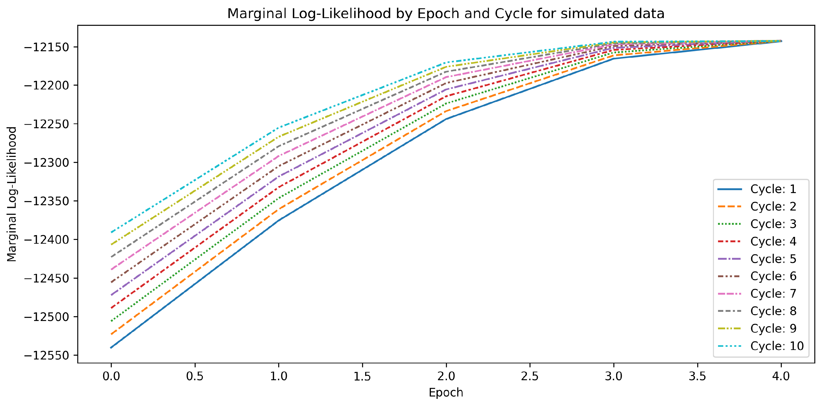
3.3. Training Algorithm

The epoch (e) describes the number of times the E-M algorithm is iterated. The cycles (c) describe the number of times the gradient descent is run in the M-step in each epoch. The training algorithm is described below in Algorithm 1:

Algorithm 1 Training Optimization algorithm

1: Input: 2:     Observation sequence $\mathcal{D}=\{{\mathbf{y}}_1,{\mathbf{y}}_2,\dots ,{\mathbf{y}}_n\}$ 3:     Initial parameters $\Phi =\{\alpha ,\beta ,\theta ,\varphi \}$ 4:     Initial state estimate ${\widehat{x}}_{0|0}$, initial covariance $P_{0|0}$ 5:     Set number of training epochs: e 6:     Set number of cycles: c 7: for $e=1$ to e do 8:    $X_{n|T},P_{n|T}$ = RTS $(Y_T,{\theta }_{old}$ {Get posterior using RTS smoother} 9:    for $c=1$ to c do 10:      $l_t$ = Monte Carlo expected log likelihood $(Y_{n|T},X_{n|T},P_{n|T})$ {Compute Expected log likelihood using posterior and loss} 11:      Back Propagation: Output of the updated parameters $\Phi$, using gradient descent on loss function. 12:    end for 13: end for

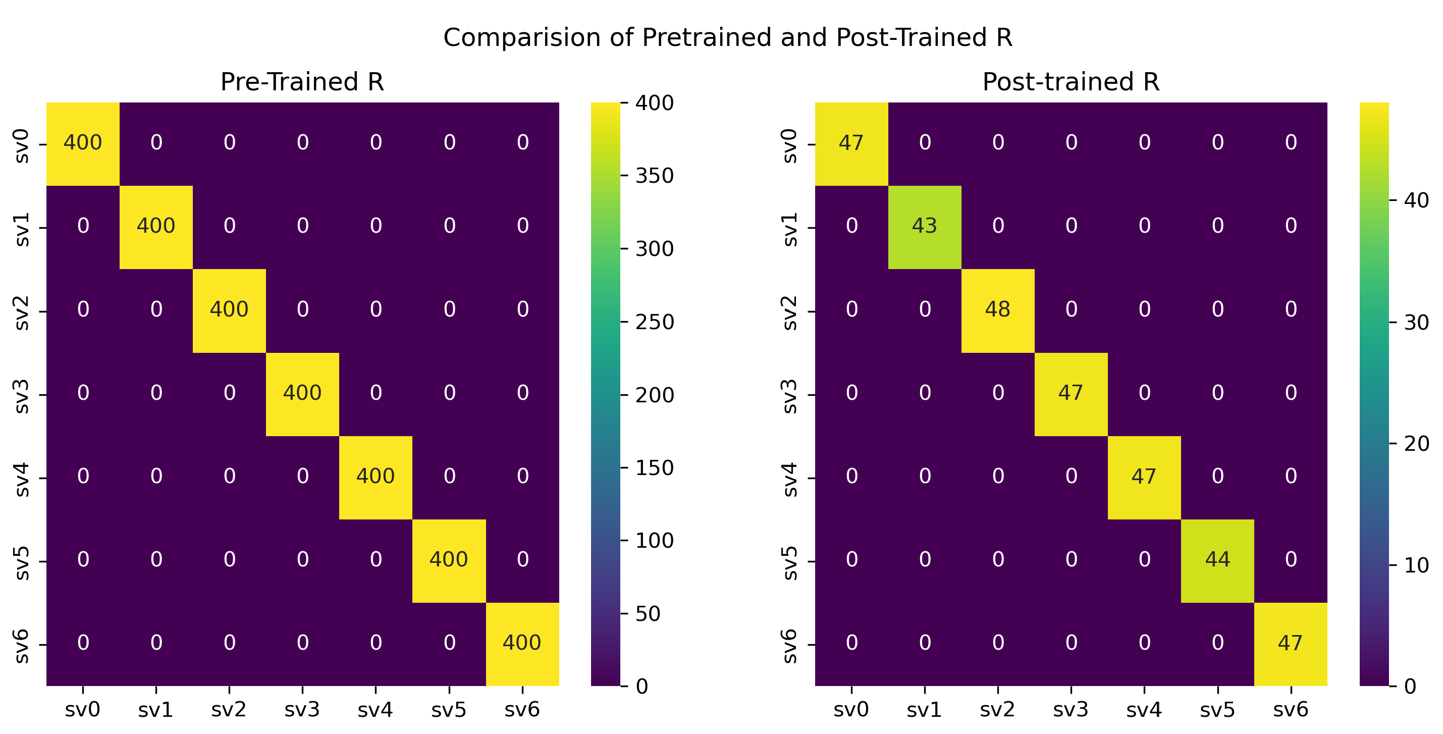
4. Results

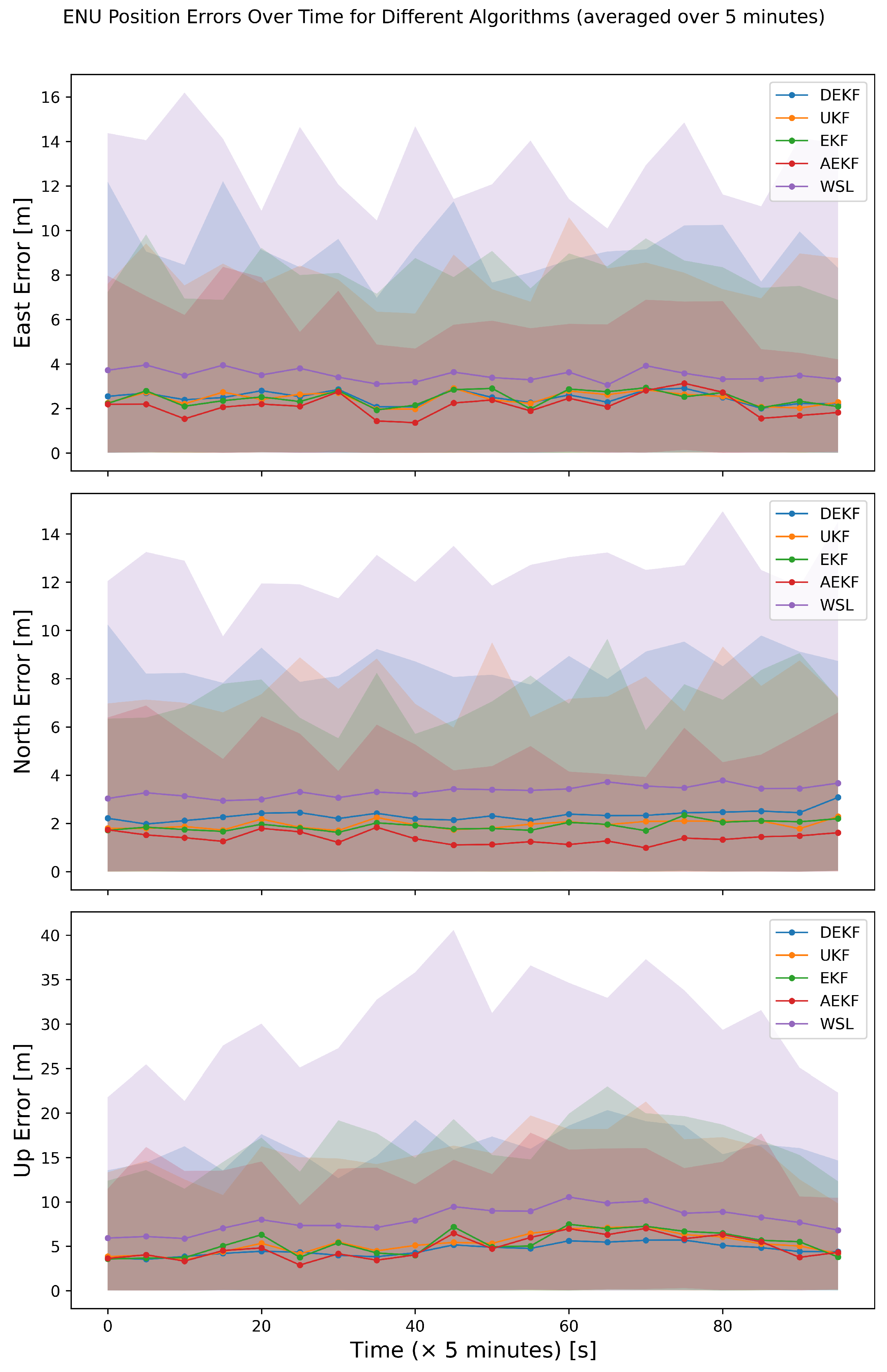
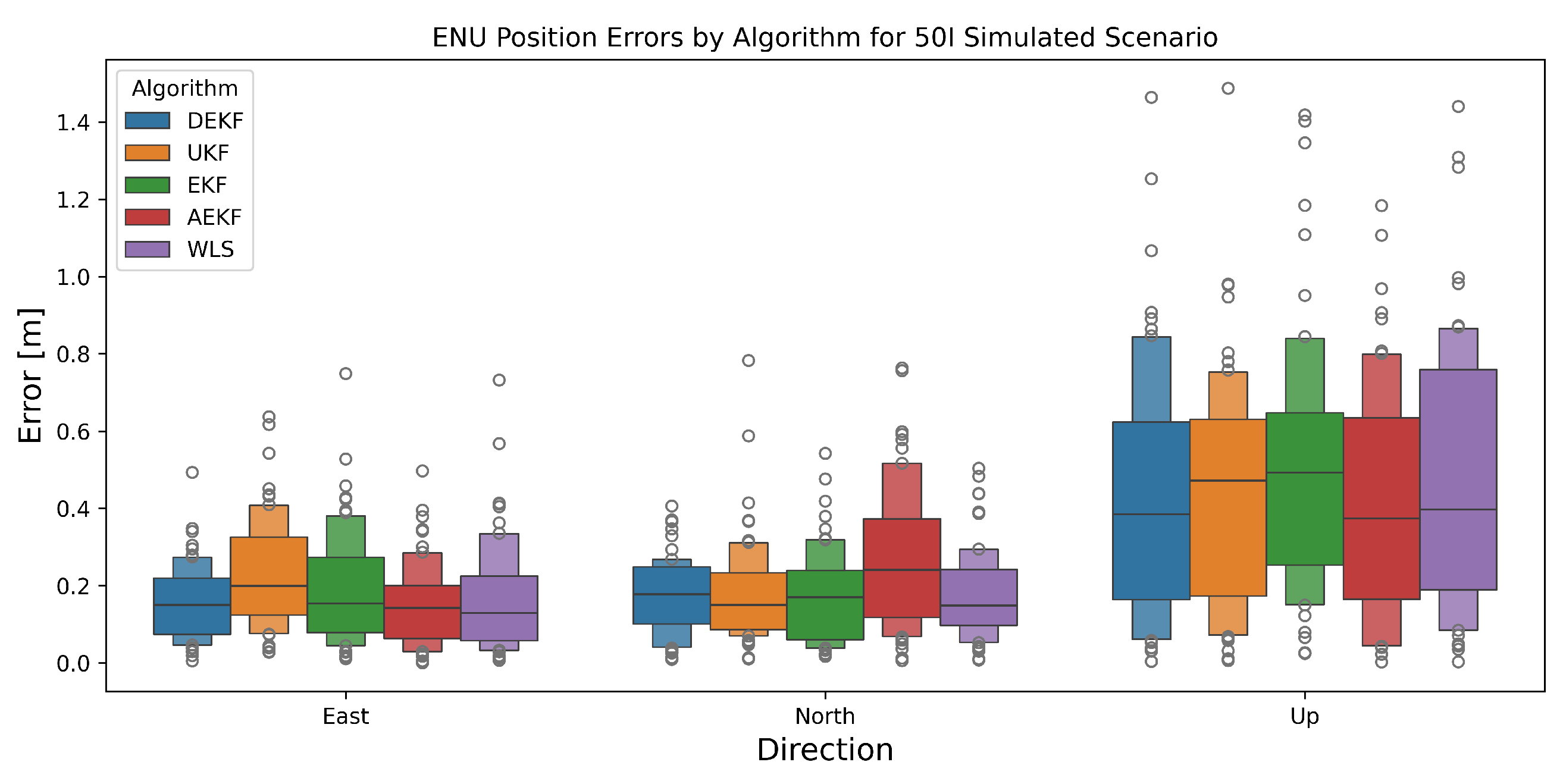
4.1. Simulation

Our hybrid differential EKF algorithm is evaluated and compared to other algorithms. In these simulations, a dynamic receiver is considered, which is subjected to noise sampled from a known probability distribution. Skydel is a software by Safran Electronics Defense, which is a GNSS simulation platform [33]. It is important to note that this software has been used previously by Elgamoudi et al. and Kujur et al. [34,35]. In our case, the Safran-Skydel GNSS simulation engine is used to model a dynamic vehicle receiving signals from the GPS constellation at the L1 and L2 frequencies. For simulation fidelity, atmospheric errors, receiver clock errors, and other delays are deliberately set to zero. The range measurements are perturbed by additive white Gaussian noise (AWGN noise), which is characterized by the following moments:

$$\mathcal{N}(\mu ,{\sigma }^{2}I)$$

(30)

where $\sigma$ denotes the standard deviation of the pseudorange measurements, and I represents the identity matrix. This noise profile ensures that the range measurements from various satellites are not correlated with each other over time. To simulate a comparable noise level observed in the real pseudorange measurements, the value of $50I$ is chosen for simulated noise levels. Initial estimates of the noise covariance matrices, as given in (6) and (7), are initialized as follows:

$$Q_0={\sigma }_q^{2}I;R_0={\sigma }_r^{2}I$$

(31)

where ${\sigma }_q$ and ${\sigma }_r$ are generally initialized based on the user’s prior information of the noise characteristics. However, we note that in our methods for simulated, static, and dynamic scenarios as seen in Section 4.2.3 and Section 4.2.4, these values were randomly chosen to demonstrate the successful convergence of noise matrices after training. In this configuration, the elements of the matrices Q and R are treated as trainable parameters, as described in (20) and (21). To enforce uncorrelated noise among range measurements from different satellites, R is parameterized as a diagonal symmetric positive matrix throughout training, as shown in Figure 2.

Unless the motion is periodic, the transition model is not parameterized, and the receiver is assumed to follow an approximately constant velocity dynamics model, represented by (14). However, the observation model is parameterized to accommodate potential biases such as equipment delays in the receiver or the signals received from the satellites. Therefore, the simplified observation model in (15) is adapted using the following equation:

$$h(\overrightarrow{r},\overrightarrow{r_j})=\left|\right|\overrightarrow{r}-\overrightarrow{r_j}\left|\right|+c\delta t_j+b_j$$

(32)

where $b_j$ denotes a constant trainable bias parameter $\varphi$. As illustrated in Figure 3, the marginal log likelihood exhibits as monotonically increasing and ultimately converging to a local minimum—consistent with the theoretical predictions.

Furthermore, analysis of the EKF innovation residuals before and after training reveals that the training process significantly reduces the autocorrelation of the residuals, as shown in Figure 4. This outcome strongly supports the consistency of the trained model with the KF assumption of uncorrelated innovations. Additionally, Figure 2 demonstrates that the estimated noise covariance matrix accurately converges to the factual covariance matrix $50I$, correcting the inaccurately initialized prior estimate. A comparative evaluation of positioning errors across different algorithms is shown in Figure 5, indicating that the variance in the horizontal position is reduced by approximately $33\%$, thus demonstrating a predictable improvement due to the alignment of the noise covariance matrix after training.

4.2. Real-World Scenarios

4.2.1. Experimental Methods

Experimentally, we train and evaluate the DEKF for triangulation across two distinct real-world scenarios, comparing its performance metrics with those of the standard KF algorithms. The following scenarios underscore the applicability of the DEKF architecture, estimating noise characteristics, learning the underlying model, or simultaneously addressing both tasks, as follows:

1.

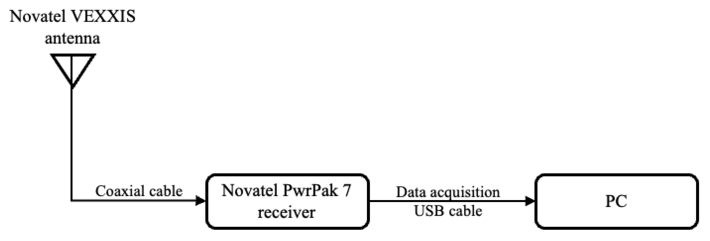
A real-world scenario featuring a stationary receiver exposed to various noise parameters with the filter tuned to detect the corresponding noise statistics. Novatel PwrPak7 GNSS receiver, NovAtel Inc., Calgary, CA, USA with Novatel VEXXIS GNSS-802 antenna, NovAtel Inc., Calgary, CA, USA is used with a PC to collect GPS measurements as shown in Figure 6 from the L1 and L2 frequencies, sampled at 1 Hz. The pictures of the Novatel antenna and Novatel receiver are shown in Figure 7.

2.

A real-world scenario involving a dynamic receiver processing GNSS signals, potentially perturbed by dynamic noise. Google Pixel 4 mobile data were used from [36] in a moving vehicle to obtain measurements from at least 7 GPS satellites at L1 frequency, sampled at 1 Hz.

4.2.2. Data Preprocessing

In the real-world datasets, the following baseline pre-processing steps are applied to GNSS receiver measurements before utilizing them in the estimation algorithms:

1.

Ionospheric Correction;

2.

Tropospheric Correction;

3.

Satellite Clock Correction.

To correct ionospheric errors, the ionospheric-free combination is used in the case of dual frequency receiver, while the Klobuchar model [37] is used for single frequency. For tropospheric delay corrections, the UNB3m neutral atmospheric model [38] is applied. In our case, for the static scenario, the above corrections are applied to the Novatel raw data. However, we note that these models may also be used for the dynamic case, when the raw data from the receiver is used for processing. Further refinements, including the utilization of unambiguous phase measurements, Doppler measurements, differencing techniques, and multi-constellation combinations, can be implemented to enhance the accuracy of state estimations further. In such instances, the basic formalism presented in this paper remains valid with some minor adjustments in the state transition and measurement functions (see Section 2.2). The true states of the real-world stationary scenario (Novatel receiver data, for our case) are computed using precise point positioning calculated from the Canadian Spatial Reference System Precise Point Positioning (CSRS-PPP) service. Whereas the PPP solution is not feasible for the dynamic scenario. This was performed to evaluate the error in the algorithms.

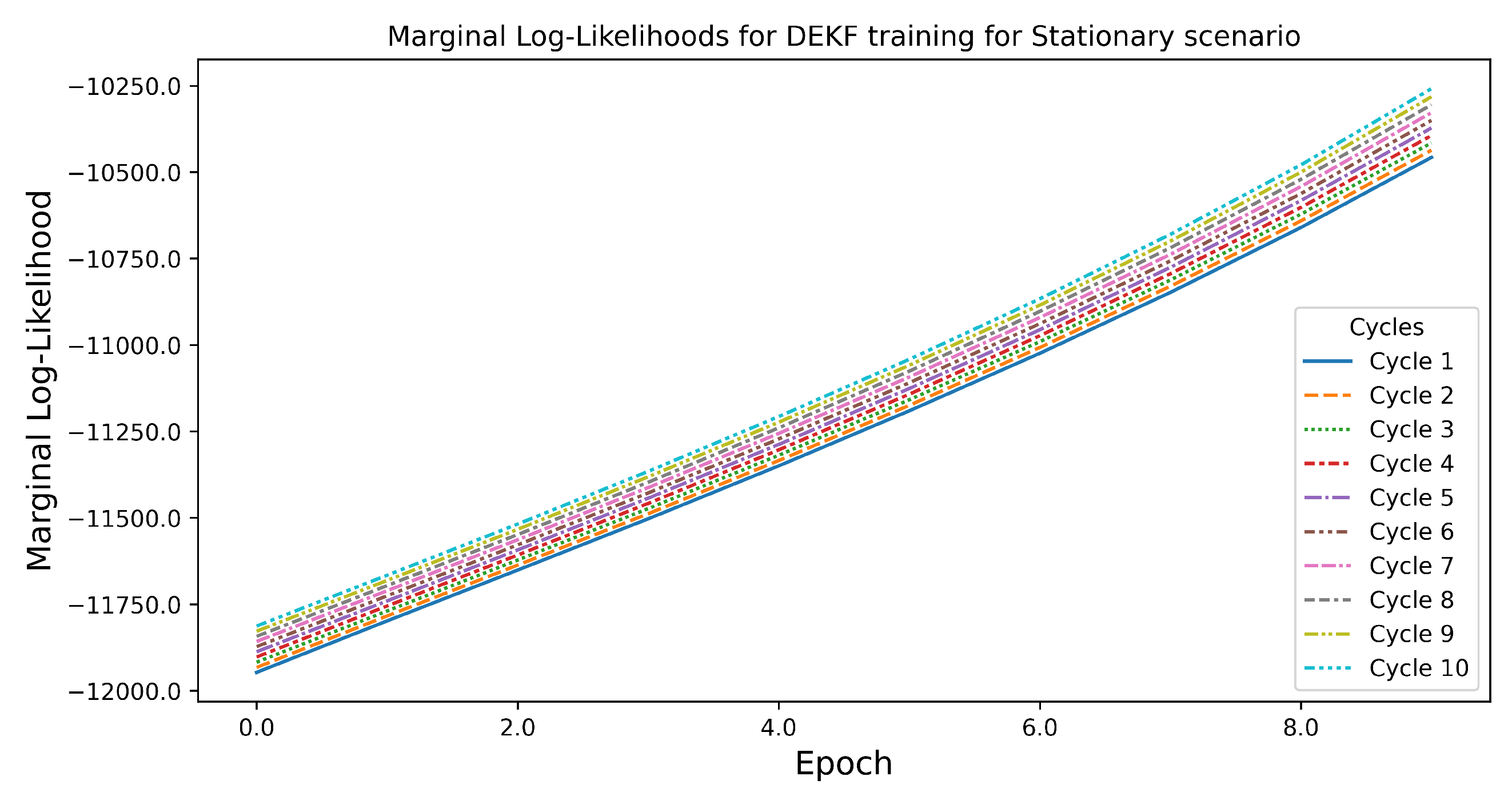
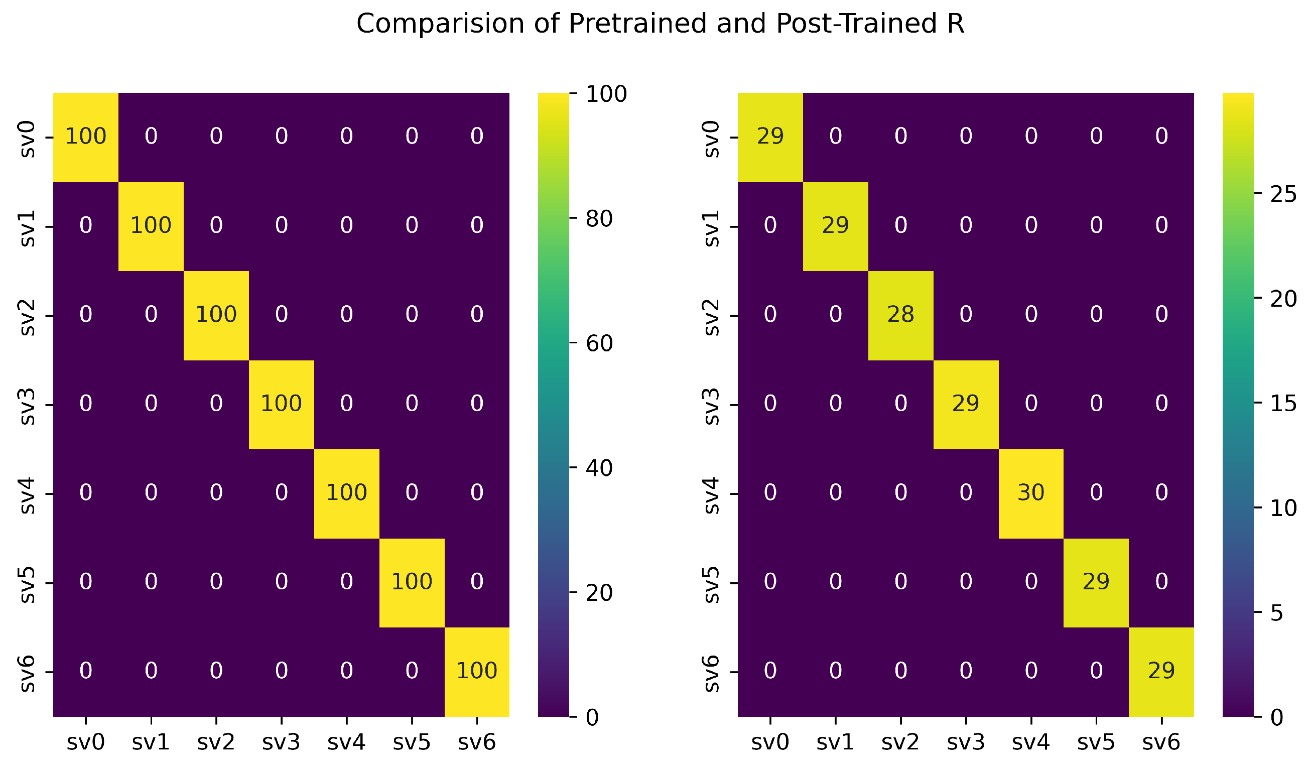
4.2.3. The Stationary Scenario

In this scenario, a Novatel PwrPak7 receiver is utilized to capture GPS measurements from L1 and L2 frequencies, sampled at 1 Hz. Unlike the simulated environment, real-world errors may exhibit non-Gaussian characteristics. However, for the purpose of state estimation, these errors are treated to be approximately Gaussian, and an EKF formulation is employed.

Following the approach used in the simulated case, the noise covariance matrices are initialized according to (31) under similar constraints. Given the static nature of the receiver, the transition function is not parameterized and known as a prior, and it adheres to a constant velocity model. However, the observation model is parameterized using (32) for the reasons mentioned above (See Section 4.1).

The dataset consists of $T=5853$ continuous pseudorange measurements collected from seven GPS satellites at a sampling rate of 1 Hz. The dataset is tuned using the first 500 observations and evaluated on the whole trajectory. Initial values of ${\sigma }_q^2=1$ and ${\sigma }_r^2=100$ are chosen for the Q and R matrices respectively, as specified in (31). The DEKF is optimized using the AdamW optimizer over 5 epochs and 10 cycles, as shown in Figure 8. The marginal log likelihood does reach the local maxima value as expected, but unlike the simulated case, it does not fully converge. This may be because of the minimal training of the DEKF for a limited real-world dataset.

Although the full convergence is not observed, as evident in Figure 9, there is an improvement in the positioning errors for all three directions. Further, the time series representation of ENU errors is provided in Section 5 (see Figure 14). Although there is a slight increase in five-minute averages of ENU errors for the “east” and “north” directions for the DEKF as compared to other algorithms, the error ranges are comparable. This shows that the DEKF is still competitive for the static scenario. Furthermore, the noise measurement matrix converges, as shown in Figure 10, eliminating the need for manual tuning, which is a prerequisite for the other algorithms.

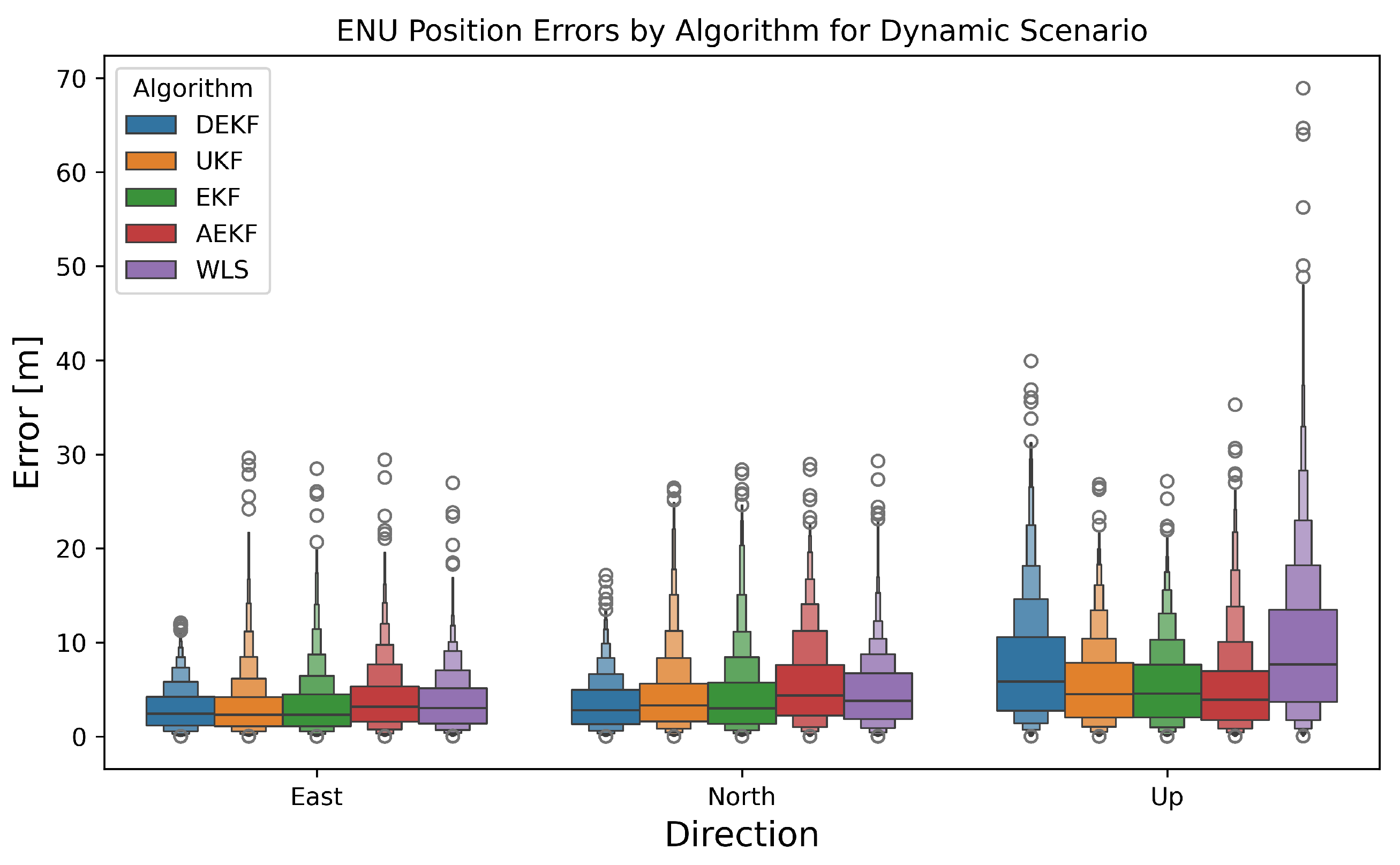
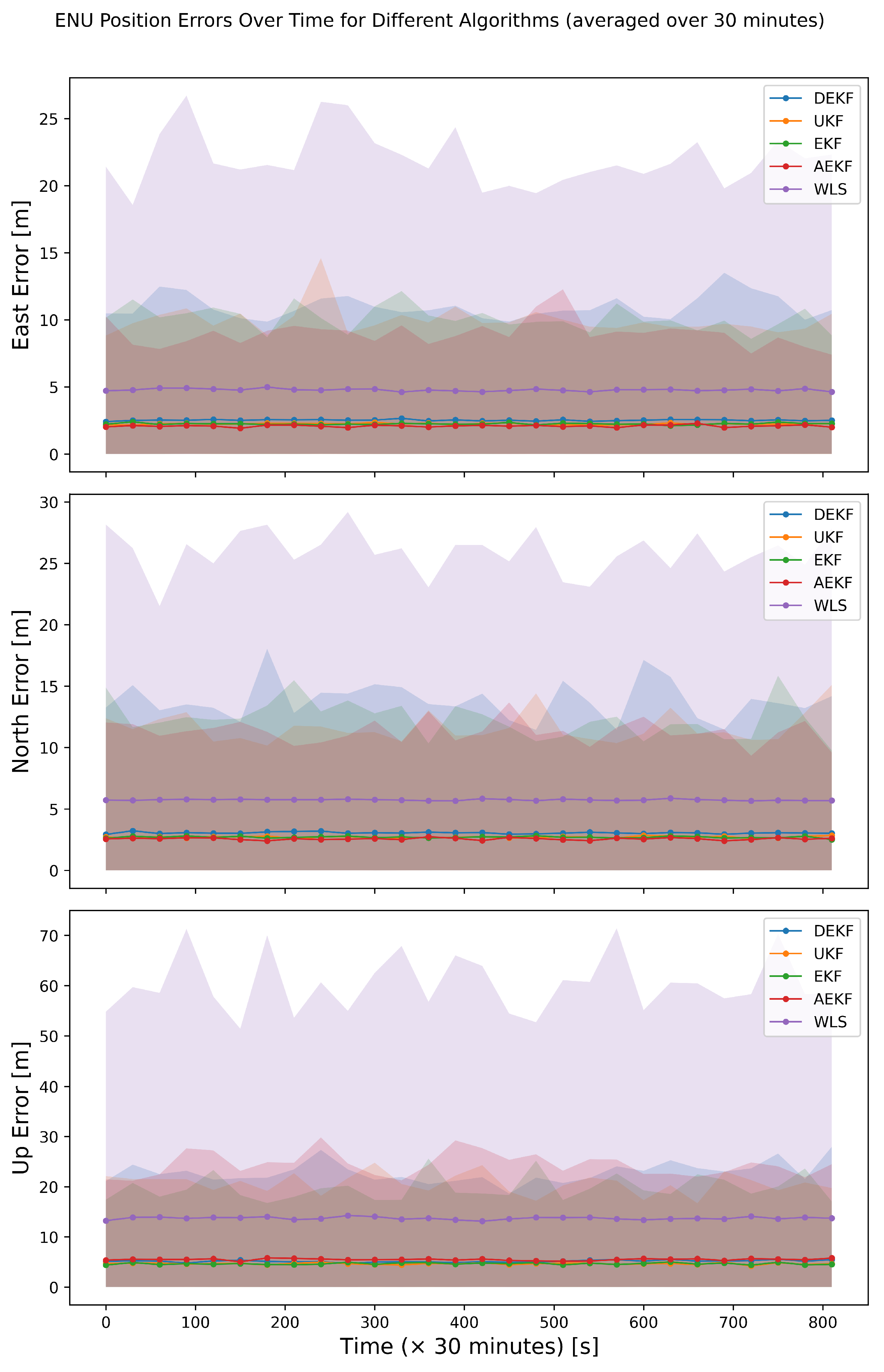
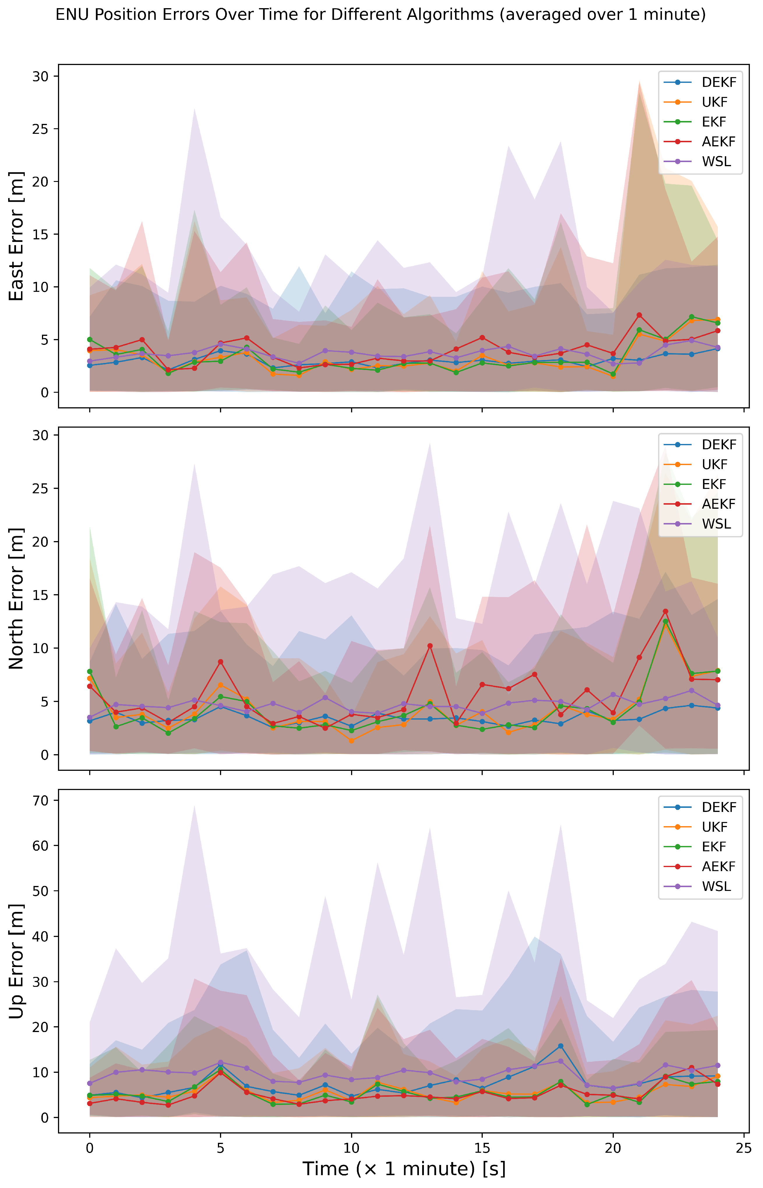
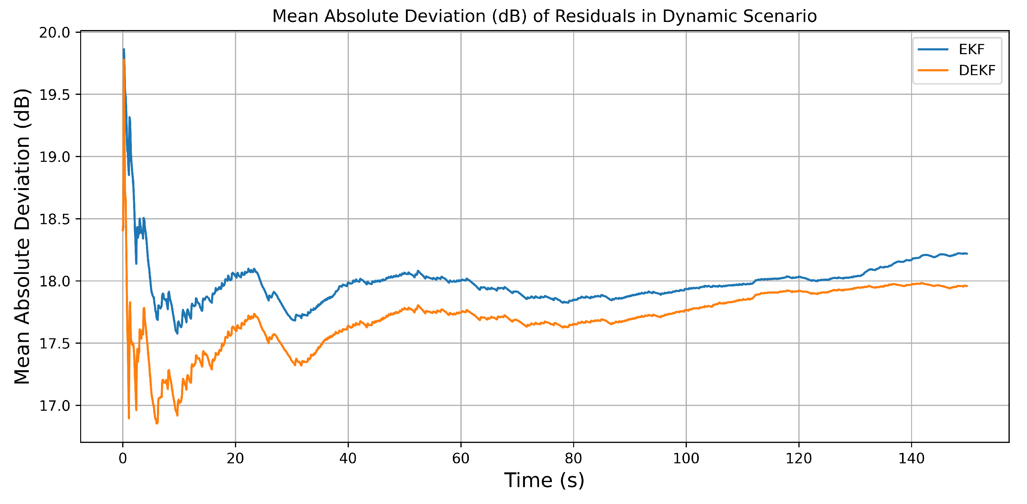
4.2.4. The Dynamic Scenario

In the dynamic case, the Google Pixel 4 mobile data were used from [36], where an Android phone was employed to obtain measurements simultaneously from the seven GPS satellites at L1 frequency, sampled at 1Hz, from a moving vehicle. Unlike the static scenario, the range measurements are significantly affected by environmental factors such as multipath effects and time-dependent noise. Similar to the simulated case, the noise covariance matrices are initialized in the form (31) with ${\sigma }_q^2=1$ and ${\sigma }_r^2=400$. The same configuration of the DEKF was used as in the static scenario; however, in this case, the measurement noise is parametrized as a complete symmetric matrix.

The dynamic dataset consists of $T=1500$ continuous pseudorange measurements collected from seven GPS satellites with approximately 25 min of dynamic data. The DEKF is fitted into tuning using the first 500 measurements and evaluated on the whole trajectory. As shown in Figure 11, the DEKF is tuned using the AdamW optimizer for 10 epochs and 5 cycles, with the marginal likelihood converging to a stable value.

As shown in Figure 12, the variance in horizontal positioning improves by 33% compared to other methods. However, compared to the simulated case, there is no significant improvement in vertical positioning, compared to the EKF, UKF, and AEKF. Perhaps, this is due to the unsupervised nature of maximum likelihood training, as it may not always lead directly to improved positioning.

5. Discussion

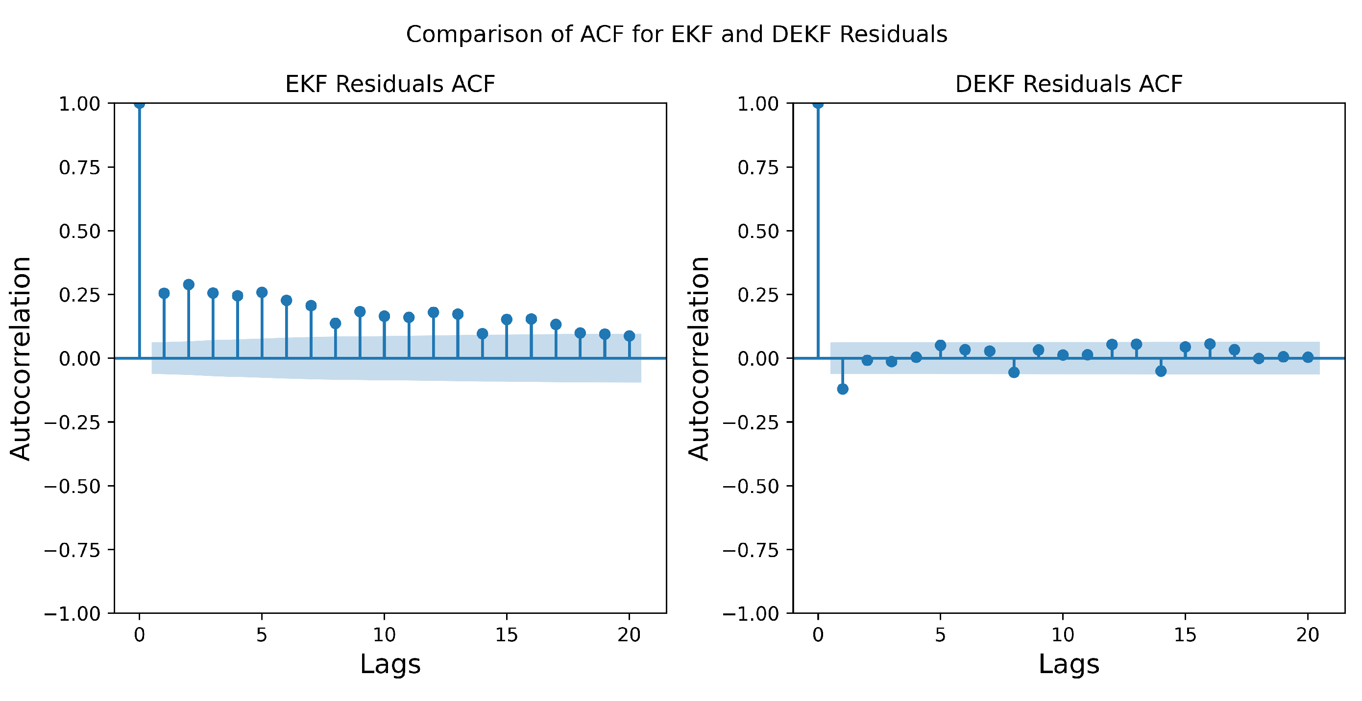
5.1. Simulated Scenario

As seen in Figure 5, the East-North-Up (ENU) positioning errors from 50 Monte Carlo simulations, showed the 33% improvement in variance due to the noise covariance matrix training. Furthermore, our analysis shown in Figure 13 represents a time series plot of the ENU errors averaged over 30 min, along with the range (minimum and maximum). This figure reveals that the error in the “up” direction for the DEKF algorithm achieves a constantly lower ENU error range as compared to all other algorithms.

5.2. Static Scenario

The experiments done with the static GNSS receiver provided the data that was subjected to our DEKF algorithm, showing a clear improvement in ENU accuracy, that is better than WLS and is at par with the other methods such as UKF, EKF, and AEKF. Figure 14 shows the time series of ENU errors for the static data with clear distinction of the improvements with the DEKF algorithm.

Figure 14. Time series of ENU errors for the static receiver scenario. The solid lines represent the averaged data, and the shaded region represents the range (minimum to maximum) of the ENU errors for every data point. The WSL method has considerably larger ranges of errors as compared to all other algorithms in all three directions, as seen in the simulated scenario in Figure 13. The DEKF algorithm maintains a competitive error range, as compared to the UKF, EKF, and AEKF throughout the measurement time.

Figure 14. Time series of ENU errors for the static receiver scenario. The solid lines represent the averaged data, and the shaded region represents the range (minimum to maximum) of the ENU errors for every data point. The WSL method has considerably larger ranges of errors as compared to all other algorithms in all three directions, as seen in the simulated scenario in Figure 13. The DEKF algorithm maintains a competitive error range, as compared to the UKF, EKF, and AEKF throughout the measurement time.

5.3. Dynamic Scenario

The improved performance with DEKF method for the real-world dynamic scenario upto 33% in the horizontal directions (E and N) was demonstrated in Figure 12. However, we have noticed no significant improvement in the "Up" direction, due to unsupervised nature of the algorithm. Furthermore, we are investigating the possible improvements in our algorithm to enhance the accuracy in the vertical direction. Figure 15 shows the spread of ENU errors over time, that is averaged every minute, representing the performance improvement with DEKF method.

The mean absolute deviation ($MAD$) is obtained by computing the average of the differences of the absolute values from the mean value in a series. In this case, this statistic is applied to the innovation (difference between measurement and prediction) of different filters. This gives a robust measure of how much the innovations deviate (on average) from their mean. Typically, this is expected to be zero if the filter is well-behaved. For the innovations given by ${\tilde{y}}_t=z_t-H{x}_t|x_{t-1}$, the $MAD$ is given by,

$$MAD={\displaystyle \frac{1}{T}}\sum _{t=1}^T|{\tilde{y}}_t-\overline{\tilde{y}}|$$

(33)

Figure 16 shows the mean absolute deviation plotted in dB scale ($10lo{g}_{10}\left(MAD\right)$) for a better visualization of the data. It illustrates the model’s consistency, with the DEKF achieving a lower $MAD$ throughout the entire time period, indicating a better fit to the measurements. In addition, it also shows the capability of the DEKF to effectively mitigate measurement error.

6. Conclusions

In this study, we introduced the Differentiable Extended Kalman Filter (DEKF), a more adaptable version of the conventional Extended Kalman Filter (EKF). We applied the DEKF to GNSS state estimation and developed a loss function based on the maximum likelihood principle. This loss function supports unsupervised filter training, allowing data-driven adjustments to model priors and discovering error statistics. We implemented a modified version of the expectation-maximization algorithm and an RTS smoother to train the DEKF algorithm. Unlike other algorithms that require true states for training, the DEKF guarantees the convergence of noise matrices, resulting in increased robustness and reliability. Moreover, the DEKF is highly versatile and can be easily extended, modified, and deployed based on specific observation models. The real-world datasets demonstrate the potential of the DEKF, with lower variance in positioning results at better than 30% improvement compared to other algorithms like the EKF, UKF, WLS, and AEKF.

Furthermore, the mean absolute deviation achieved using our method is consistently better than the performance obtained by the conventional EKF method by up to an order of magnitude. We found that the DEKF is particularly suitable for environments where we have limited knowledge of the actual state and unknown noise types, as demonstrated in the results section. Therefore, given its strength and versatility, the DEKF method within a neural network adaptation has the potential for various applications where the true state of the system and the noises are unknown.

References

- Hofmann-Wellenhof, B.; Lichtenegger, H.; Wasle, E. GNSS—Global Navigation Satellite Systems: GPS, GLONASS, Galileo, and More; Springer Science & Business Media: Berlin/Heidelberg, Germany, 2007. [Google Scholar]
- Seeber, G. Satellite Geodesy; Walter de Gruyter: Berlin, Germany, 2003. [Google Scholar]
- Teunissen, P.J.; Montenbruck, O. Springer Handbook of Global Navigation Satellite Systems; Springer: Berlin/Heidelberg, Germany, 2017; Volume 10. [Google Scholar]
- Iqbal, A.; Mahmood, H.; Farooq, U.; Kabir, M.A.; Asad, M.U. An Overview of the Factors Responsible for GPS Signal Error: Origin and Solution. In Proceedings of the 2009 International Conference on Wireless Networks and Information Systems, Shanghai, China, 28–29 December 2009; pp. 294–299. [Google Scholar] [CrossRef]
- Kaplan, E.; Hegarty, C. Understanding GPS/GNSS: Principles and Applications, 3rd ed.; GNSS Technology and Applications Series; Artech House Publishers: London, UK, 2017; ISBN 9781630814427. [Google Scholar]
- Gruber, M. An Approach to Target Tracking; Technical Note 1967-8; Massachusetts Institute of Technology Lincoln Laboratory: Lexington, MA, USA, 1967. [Google Scholar]
- Julier, S.; Uhlmann, J. Unscented filtering and nonlinear estimation. Proc. IEEE 2004, 92, 401–422. [Google Scholar] [CrossRef]
- Li, K.; Zhou, G.; Kirubarajan, T. A general model-based filter initialization approach for linear and nonlinear dynamic systems. Digit. Signal Process. 2021, 111, 102978. [Google Scholar] [CrossRef]
- Guo, Y.; Chai, S.; Cui, L. GNSS Precise Point Positioning Based on Dynamic Kalman Filter with Attenuation Factor. In Proceedings of the 2018 37th Chinese Control Conference (CCC), Wuhan, China, 25–27 July 2018; pp. 4734–4738. [Google Scholar] [CrossRef]
- Xiao, G.; Yang, C.; Wei, H.; Xiao, Z.; Zhou, P.; Li, P.; Dai, Q.; Zhang, B.; Yu, C. PPP ambiguity resolution based on factor graph optimization. GPS Solut. 2024, 28, 178. [Google Scholar] [CrossRef]
- Kanhere, A.V.; Gupta, S.; Shetty, A.; Gao, G. Improving GNSS Positioning Using Neural-Network-Based Corrections. Navig. J. Inst. Navig. 2022, 69. [Google Scholar] [CrossRef]
- Lee, J.; Lee, Y.; Kim, J.; Kosiorek, A.; Choi, S.; Teh, Y.W. Set Transformer: A Framework for Attention-based Permutation-Invariant Neural Networks. In Proceedings of the 36th International Conference on Machine Learning, Long Beach, CA, USA, 9–15 June 2019; Proceedings of Machine Learning Research. Chaudhuri, K., Salakhutdinov, R., Eds.; Volume 97, pp. 3744–3753. [Google Scholar]
- Liu, Z.; Liu, J.; Xu, X.; Wu, K. DeepGPS: Deep Learning Enhanced GPS Positioning in Urban Canyons. IEEE Trans. Mob. Comput. 2024, 23, 376–392. [Google Scholar] [CrossRef]
- Zhang, G.; Xu, P.; Xu, H.; Hsu, L.T. Prediction on the Urban GNSS Measurement Uncertainty Based on Deep Learning Networks With Long Short-Term Memory. IEEE Sens. J. 2021, 21, 20563–20577. [Google Scholar] [CrossRef]
- Hochreiter, S.; Schmidhuber, J. Long short-term memory. Neural Comput. 1997, 9, 1735–1780. [Google Scholar] [CrossRef]
- Mohanty, A.; Gao, G. Learning GNSS Positioning Corrections for Smartphones Using Graph Convolution Neural Networks. Navig. J. Inst. Navig. 2023, 70. [Google Scholar] [CrossRef]
- Kloss, A.; Martius, G.; Bohg, J. How to train your differentiable filter. Auton. Robot. 2021, 45, 561–578. [Google Scholar] [CrossRef]
- Haarnoja, T.; Ajay, A.; Levine, S.; Abbeel, P. Backprop KF: Learning Discriminative Deterministic State Estimators. arXiv 2016, arXiv:arXiv:1605.07148. [Google Scholar]
- Liu, W.; Lai, Z.; Bacsa, K.; Chatzi, E. Neural extended Kalman filters for learning and predicting dynamics of structural systems. Struct. Health Monit. 2024, 23, 1037–1052. [Google Scholar] [CrossRef]
- Revach, G.; Shlezinger, N.; Ni, X.; Escoriza, A.L.; van Sloun, R.J.G.; Eldar, Y.C. KalmanNet: Neural Network Aided Kalman Filtering for Partially Known Dynamics. IEEE Trans. Signal Process. 2022, 70, 1532–1547. [Google Scholar] [CrossRef]
- Guo, Y.; Vouch, O.; Zocca, S.; Minetto, A.; Dovis, F. Enhanced EKF-based time calibration for GNSS/UWB tight integration. IEEE Sens. J. 2022, 23, 552–566. [Google Scholar] [CrossRef]
- Shumway, R.H.; Stoffer, D.S. An Approach to Time Series Smoothing and Forecasting Using the EM Algorithm. J. Time Ser. Anal. 1982, 3, 253–264. [Google Scholar] [CrossRef]
- Li, X.; Wang, Z.; Zhang, L. Co-estimation of capacity and state-of-charge for lithium-ion batteries in electric vehicles. Energy 2019, 174, 33–44. [Google Scholar] [CrossRef]
- Kiers, H.A. Weighted least squares fitting using ordinary least squares algorithms. Psychometrika 1997, 62, 251–266. [Google Scholar] [CrossRef]
- Li, X.; Huang, J.; Li, X.; Shen, Z.; Han, J.; Li, L.; Wang, B. Review of PPP–RTK: Achievements, challenges, and opportunities. Satell. Navig. 2022, 3, 28. [Google Scholar] [CrossRef]
- Sunahara, Y.; Kohji, Y. An approximate method of state estimation for non-linear dynamical systems with state-dependent noise. Int. J. Control 1970, 11, 957–972. [Google Scholar] [CrossRef]
- Triantafyllopoulos, K. The Kalman Filter. In Bayesian Inference of State Space Models: Kalman Filtering and Beyond; Springer International Publishing: Cham, Switzerland, 2021; pp. 63–109. [Google Scholar] [CrossRef]
- Stone, J.V. Bayes’ Rule: A tutorial Introduction to Bayesian Analysis; Sebtel Press, 2013. [Google Scholar] [CrossRef]
- Baydin, A.G.; Pearlmutter, B.A.; Radul, A.A. Automatic differentiation in machine learning: A survey. arXiv 2015, arXiv:1502.05767. [Google Scholar]
- Zaheer, R.; Shaziya, H. A Study of the Optimization Algorithms in Deep Learning. In Proceedings of the 2019 Third International Conference on Inventive Systems and Control (ICISC), Coimbatore, India, 10–11 January 2019; pp. 536–539. [Google Scholar] [CrossRef]
- Dempster, A.P.; Laird, N.M.; Rubin, D.B. Maximum Likelihood from Incomplete Data via the EM algorithm. J. R. Stat. Soc. Ser. (Methodol.) 1977, 39, 1–38. [Google Scholar] [CrossRef]
- Rauch, H.E.; Tung, F.; Striebel, C.T. Maximum likelihood estimates of linear dynamic systems. AIAA J. 1965, 3, 1445–1450. [Google Scholar] [CrossRef]
- Safran Electronics & Defense. User Manual—Skydel Software Defined GNSS Simulator. 2024. Available online: https://safran-navigation-timing.com/document/user-manual-skydel-software-defined-gnss-simulator/ (accessed on 17 April 2025).
- Elgamoudi, A.; Benzerrouk, H.; Elango, G.A.; Landry, R.J. Quasi-real RFI source generation using orolia skydel LEO satellite simulator for accurate geolocation and tracking: Modeling and experimental analysis. Electronics 2022, 11, 781. [Google Scholar] [CrossRef]
- Kujur, B.; Khanafseh, S.; Pervan, B. Experimental validation of optimal INS monitor against GNSS spoofer tracking error detection. In Proceedings of the 2023 IEEE/ION Position, Location and Navigation Symposium (PLANS), Monterey, CA, USA, 24–27 April 2023; IEEE: Piscataway, NJ, USA, 2023; pp. 592–596. [Google Scholar]
- Fu, G.M.; Khider, M.; Van Diggelen, F. Android raw GNSS measurement datasets for precise positioning. In Proceedings of the 33rd International Technical Meeting of the Satellite Division of the Institute of Navigation (ION GNSS+ 2020), Online, 22–25 September 2020; pp. 1925–1937. [Google Scholar]
- Klobuchar, J.A. Ionospheric Time-Delay algorithm for Single-Frequency GPS Users. IEEE Trans. Aerosp. Electron. Syst. 1987, AES-23, 325–331. [Google Scholar] [CrossRef]
- Leandro, R.F.; Santos, M.C.; Langley, R.B. UNB Neutral Atmosphere Models: Development and Performance. In Proceedings of the 2006 National Technical Meeting of the Institute of Navigation, Monterey, CA, USA, 18–20 January 2006. [Google Scholar]
Disclaimer/Publisher’s Note: The statements, opinions and data contained in all publications are solely those of the individual author(s) and contributor(s) and not of MDPI and/or the editor(s). MDPI and/or the editor(s) disclaim responsibility for any injury to people or property resulting from any ideas, methods, instructions or products referred to in the content. |
© 2025 by the authors. Licensee MDPI, Basel, Switzerland. This article is an open access article distributed under the terms and conditions of the Creative Commons Attribution (CC BY) license (https://creativecommons.org/licenses/by/4.0/).
Share and Cite
Verma, J.; Bhattarai, N.; Bandi, T.N. Hybrid Filtering Technique for Accurate GNSS State Estimation. Remote Sens. 2025, 17, 1552. https://doi.org/10.3390/rs17091552
Verma J, Bhattarai N, Bandi TN. Hybrid Filtering Technique for Accurate GNSS State Estimation. Remote Sensing. 2025; 17(9):1552. https://doi.org/10.3390/rs17091552
Chicago/Turabian StyleVerma, Jahnvi, Nischal Bhattarai, and Thejesh N. Bandi. 2025. "Hybrid Filtering Technique for Accurate GNSS State Estimation" Remote Sensing 17, no. 9: 1552. https://doi.org/10.3390/rs17091552
APA StyleVerma, J., Bhattarai, N., & Bandi, T. N. (2025). Hybrid Filtering Technique for Accurate GNSS State Estimation. Remote Sensing, 17(9), 1552. https://doi.org/10.3390/rs17091552