Abstract
The carbon cycle of forest ecosystems is a component of the global terrestrial ecosystem carbon cycle, and the productivity of forest ecosystems is significantly influenced by vegetation phenology. In this investigation, we simulated the spatiotemporal trends of the carbon cycle in forest ecosystems in Hangzhou between 2001 and 2020 by means of the phenology-driven InTEC model and analyzed the mechanisms of carbon cycle changes in response to phenological changes. The results of this study suggested that the gross primary productivity (GPP), the net primary production (NPP), and the net ecosystem productivity (NEP) have obvious heterogeneity in spatiotemporal distribution, and the tendency of the start of the growing season (SOS) advancement, the end of the growing season (EOS) postponement, and the length of the growing season (LOS) lengthening is significant for a GPP increase with positive effects. Both phenology and climate have direct impacts on carbon cycle changes, while climate change indirectly affects carbon cycle changes through phenology changes.
1. Introduction
Vegetation phenology refers to the stages of plant development, such as germination, leaf growth, flowering, fruiting, and defoliation, and their regular changes in response to climate variations [1,2,3,4]. While both forest and crop phenology follow seasonal cycles, there are fundamental differences between them, primarily in temporal scale and ecological function [5]. Crop phenology operates on a shorter annual cycle, directly managed by human agricultural activities, whereas forest phenology unfolds over much longer timescales and is influenced primarily by natural environmental factors [6,7]. Unlike crops, which are often harvested within a single season, forest ecosystems exhibit continuous carbon accumulation over decades, making phenology a critical factor in long-term carbon balance assessments [8,9,10,11]. Research has underscored the critical role of phenology in monitoring ecosystem responses to climate dynamics. For instance, Piao found that rising temperatures lead to earlier leaf unfolding and delayed leaf senescence, thereby lengthening the growing season [11]. Similarly, Schwartz observed that accelerated spring warming in temperate regions of the Northern Hemisphere triggers earlier phenological events [8]. These shifts have significant consequences for ecosystem water, heat, and carbon cycles [12]. Therefore, it is important to understand the impacts of phenological changes and climate change on carbon cycling in forest ecosystems [13,14].
Vegetation phenology is a key factor influencing the productivity of forest ecosystems, and its variations can provide valuable insights into the carbon balance of terrestrial ecosystems [15,16]. The length of the growing season in forests, defined by the period between leaf-out in spring and senescence in autumn, is a crucial determinant of forest productivity and carbon sequestration potential [15,17,18]. Gross primary production (GPP), net primary productivity (NPP), and net ecosystem productivity (NEP) are key indicators of the carbon cycle, measuring the total carbon captured by plants through photosynthesis [19,20,21]. Keenan [22] suggested that warming promotes an early spring and late fall, increasing the LOS and thus, carbon storage in temperate forests. Piao [23] examined the effect of phenology on C flux between 1980 and 2002 in the Northern Hemisphere, concluding that LOS was closely tied to GPP, with a longer LOS ultimately promoting vegetation growth.
Deforestation is a critical factor influencing the forest carbon cycle, as it leads to significant carbon emissions by reducing biomass and altering soil carbon dynamics [24,25]. Large-scale deforestation has been linked to increased atmospheric CO2 concentrations and reduced global carbon sequestration capacity [26]. Remote sensing has the characteristics of high resolution and wide coverage, which is helpful to accurately assess forest cover change and carbon cycle monitoring [27,28]. The forest ecosystem carbon cycle is a key component of the global terrestrial carbon cycle, and carbon cycle simulations have become essential for studying this process [29]. Forest carbon cycle models are mainly divided into statistical models, remote sensing parameter models, and process-based models. Statistical models use observed data to reveal patterns in carbon cycling through statistical analysis. Remote sensing parameter models are based on remote sensing data, while process-based models optimize parameters by integrating climatic conditions, soil, vegetation physiological, and geographic location. Notable examples of process-based models include the TEM, CENTURY, BIOME-BGC, BEPS, and InTEC models. Among these, the InTEC model is particularly effective as it simulates both the carbon and water cycles by incorporating a variety of environmental variables. The integration of remote sensing technology with process-based models, such as InTEC, has proven to be a powerful tool for simulating and monitoring the forest carbon cycle. Currently, as one of the models suitable for simulating the carbon cycle in forest ecosystems, it is widely used in China [15,30], the United States [31,32], Canada [18,33], and other regions, all of which have obtained better simulation results.
Hangzhou, renowned for its rich ecological and cultural heritage, possesses extensive forest resources that play a significant role in regional carbon sequestration and climate regulation [34]. The region’s diverse forest ecosystems, influenced by a subtropical monsoon climate, provide a unique case study for assessing the impacts of phenological changes on carbon cycling. In the present study, we simulated the spatiotemporal trends of the carbon cycle from 2001 to 2020 in Hangzhou forest ecosystems by using the phenology-driven InTEC model and combining the data of forest distribution, leaf area index, and soil. Additionally, we analyzed how phenological variations influence shifts in carbon cycling mechanisms.
2. Materials and Methods
2.1. Study Region
Hangzhou is situated in the eastern part of Zhejiang Province (Figure 1). Its four distinct seasons are indicative of a subtropical monsoon climate. The annual average temperature in Hangzhou ranges from approximately 16 °C to 18 °C, with hot and rainy summers and mild, humid winters. The annual average precipitation is between 1100 and 1600 mm. Hangzhou is renowned for its abundant forest resources and extensive urban greenbelts, with a forest coverage rate exceeding 70%. Its distinct subtropical monsoon climate and rich natural resources provide a unique context for studying carbon cycling within forest ecosystems.
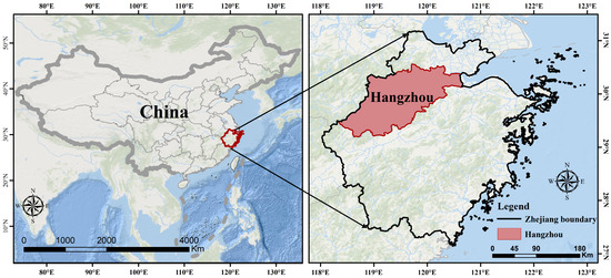
Figure 1.
Geographic position of the study region.
2.2. Data Processing
2.2.1. Meteorological Data
Meteorological data for 2001–2020 were acquired from the China Meteorological Science Data Sharing Service Network (http://data.cma.cn/), which provides daily surface meteorological data for Zhejiang Province and its neighboring regions. To ensure spatial continuity, data from surrounding provinces and cities were interpolated using an inverse distance-weighted algorithm. The Hangzhou data was then extracted to generate daily meteorological raster data with the same resolution as the MODIS EVI. Temperature data were adjusted for elevation using digital elevation model (DEM) data, assuming that the temperature decreases with elevation at a decreasing rate of 6.5 °C km−1 [35]. The total solar radiance was modeled according to Ju [36], and utilizes the sunshine time of each station’s measurements to simulate solar radiation. Annual-scale meteorological data including Pre, Tmax, Tmin, Rad, and relative humidity (Rhu) were obtained by averaging the daily-scale data.
2.2.2. Soil Data
Soil data included eight types: soil texture, soil depth, soil total organic carbon storage, hydrolytic nitrogen, nitrogen, phosphorus, potassium, and PH. The soil textures were sourced from the China Soil Database (http://vdb3.soil.csdb.cn/), managed by the Soil Sub-Center of the Nanjing Soil Research Institute, Chinese Academy of Sciences. The other soil attribute data were derived from field measurements of 888 sample plots surveyed across Zhejiang Province. Using the sample data for soil depth, soil total organic carbon stock, hydrolyzed nitrogen, total nitrogen, phosphorus, potassium, and PH, ordinary kriging interpolation was used to generate spatial distribution maps of the soil data in Zhejiang. The study area extent was then extracted, and the spatial resolution was standardized to 250 m to align with the MODIS EVI. In addition, the InTEC model also requires soil data such as the effective water-holding capacity of soil, soil bulk weight, and soil wilting point as input parameters. The soil bulk weight was calculated by the Brooks–Corey model, as improved by Saxton, incorporating soil texture data [37]. The effective water-holding capacity and wilting point were also calculated based on soil texture data [38].
2.2.3. Forest Distribution Map
The forest distribution map for 2001–2020 was derived from the annual China Land Cover Dataset (CLCD), with a spatial resolution of 30 m and an accuracy of 79.31% [34,39]. Using the land cover classification map as a reference, a reflectance mask was first converted into a minimal noise fraction (MNF). The remaining piece of the forested terrain was then isolated from the MNF scatterplot using the pixel purity index approach. The final distribution of the forest distribution map was determined through a combination of the fully constrained least squares method and the hybrid pixel decomposition method, using the land-use data [34,40,41,42].
2.2.4. Phenology Data
Phenology data were fitted to EVI time series through the opensource software TIMESAT 3.3 and extracted by the dynamic threshold method. The method mainly calculates phenological parameters by setting a specific ratio that exceeds the distance between the maximum and minimum values in the rising or falling stages of vegetation index. The thresholds of vegetation growth start and vegetation growth end are set at 30% and 15%, respectively [34].
2.3. Analysis of Spatiotemporal Trends in the Carbon Cycle
In the present research, spatiotemporal trends were calculated using Theil–Sen (TS) regression [43,44,45,46]. A nonparametric technique for calculating trends, TS regression offers a reliable estimate of the data’s trend and is particularly useful for examining the trend of lengthy time series of data [47,48].
If β > 0, it demonstrates an increasing trendency in the parameter and vice versa for a declining trendency.
In order to analyze whether β is significant or not, we used MK to test the significance of the trend over time [49,50,51]. The MK test program first defines the test statistic S:
where sgn ( ) is a sign function and is calculated as follows:
Next, the standard normal system variable Z is calculated as the following formula:
where n is the number of data.
2.4. Coefficient of Variation
The coefficient of variation (CV) is used to characterize the data, which is the ratio of standard deviation to the mean. The more variable the data, the lower the CV value indicates greater stability in the data. It makes use of the following expression:
where i refers to the year (i = 1, 2, …, n), n represents the number of data in the sequence, xi is the productivity value in year i, and is the average productivity value.
2.5. InTEC Model for Incorporating Phenology
2.5.1. Introduction to the InTEC Model
To simulate carbon dynamics in forest ecosystems at annual scales, the Integrated Terrestrial Ecosystem Carbon Income and Expenditure (InTEC) Model [18,52,53] was developed. The model is able to respond to the influence of phenological changes, forest disturbances, and climate change on carbon and nitrogen cycling in forest ecosystems [54]. Driven by spatial distribution data [55], the InTEC model has been widely used in the simulation of spatial distribution of carbon sources and sinks in forest ecosystems [30]. The InTEC model works as shown in Figure 2.
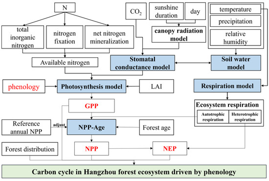
Figure 2.
The run of InTEC model.
2.5.2. InTEC Model Input Parameters
The main input parameters of the InTEC model included meteorological data, leaf area index, forest age, forest distribution map, phenology, reference year NPP, soil texture, effective soil water holding capacity, soil bulk weight, soil wilting point, CO2 concentration data, and nitrogen deposition data. In this study, the spatial resolution of the data was standardized to 250 m × 250 m, and the input data are shown in Table 1.

Table 1.
Input data in InTEC model.
2.6. Structural Equation Modeling
To better understand the relative importance of climate change and phenology change on the carbon cycle, this study assessed the direct and indirect effects of carbon cycle factors in Hangzhou forest ecosystem using structural equation modeling (SEM). SEM is particularly effective in handling multicollinearity or a small sample capacity, as it enables the simultaneous estimation of both the potential factors and observational indicators of the model. The calculation steps are as follows:
First, external estimates of the hidden variables are computed:
where is the weight and * denotes the normalization of the estimate.
Then, the internal estimate of the hidden variable is calculated:
where is the internal weight, sign is the sign function, is the correlation coefficient between the external estimator and , is the weight vector, and n is the observation sample.
Finally, the final obtained by weight iteration is used as an estimate of the hidden variable , and based on the obtained , the pass-through coefficients in the structural model are estimated by ordinary least squares.
The construction of the partial least squares pass-through model for this study is displayed in Table 2.
Table 2.
Construction of PLS path model.
3. Results
3.1. Spatiotemporal Simulation of Forest Carbon Cycle
Based on the improved InTEC model, the carbon cycle of forest ecosystems in Hangzhou was simulated for 20 years from 2001 to 2020 by integrating the climatic inversion data of Hangzhou forests into the InTEC model. The result is displayed in Figure 3, Figure 4 and Figure 5, which show the spatiotemporal distribution of GPP, NPP, and NEP.
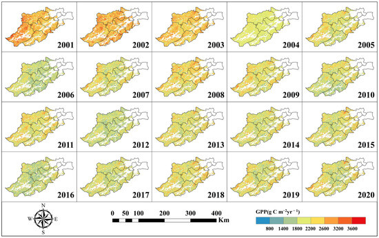
Figure 3.
GPP spatial distribution.
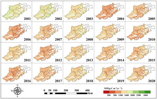
Figure 4.
NPP spatial distribution.
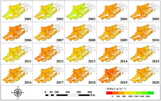
Figure 5.
NEP Spatial distribution.
As shown in Figure 3, Figure 4 and Figure 5, the spatiotemporal distributions of GPP, NPP, and NEP were obviously heterogeneous, with higher values concentrated in the southeast and northwest region, while lower values are observed in the southwest. Additionally, significant temporal variability was evident within the same region across different years.
Based on Figure 3, Figure 4 and Figure 5, the calculation can obtain the trend of the interannual average GPP, NPP, and NEP of Hangzhou forests from 2001–2020, as shown in Figure 6. Analyzing Figure 6, we can see that the annual mean GPP, NPP, and NEP all show a pronounced decreasing trend. Specifically, the annual mean GPP decreased at a rate of 22.29 g C m−2yr−1 (p < 0.01), the annual mean NPP decreased at a rate of 9.88 g C m−2yr−1, and the annual mean NEP decreased at a rate of 15.84 g C m−2yr−1 (p < 0.05).
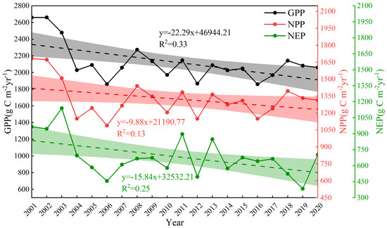
Figure 6.
Trends in Hangzhou’s forests’ yearly average GPP, NPP, and NEP values, 2001–2020.
3.2. Spatial Change Trends of Carbon Cycle in Forest Ecosystems of Hangzhou
Figure 7 illustrates the spatial distribution of the annual mean values and coefficients of variation (CVs) for GPP, NPP, and NEP in Hangzhou’s forest ecosystems, based on a spatiotemporal simulation of the carbon cycle. Figure 7a,c,e depict the spatial patterns of the annual mean values for GPP, NPP, and NEP, respectively, while Figure 7b,d,f present their corresponding CV distributions. The annual mean GPP (Figure 7a) is higher in the northwest compared to the southeast, with slightly lower values observed in the central region. The CV of GPP (Figure 7b) exhibits clear spatial heterogeneity, showing generally lower values in the northwest. The annual mean NPP (Figure 7c) demonstrates spatial variability, with higher values in the east compared to the west, and in the north compared to the south. The CV of NPP (Figure 7d) follows a similar spatial pattern, with larger variations in the eastern and southern regions. As shown in Figure 7e, NEP values are higher in the southeast than in the northwest, and slightly higher in the east compared to the west. The CV of NEP (Figure 7f) is somewhat elevated in the southwestern region.
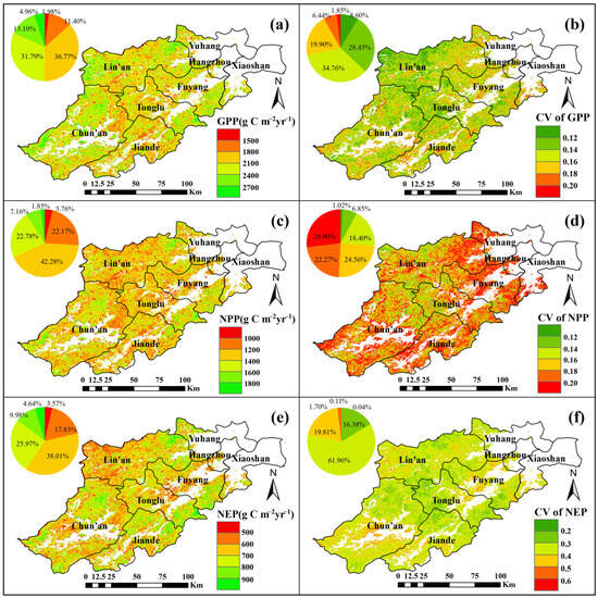
Figure 7.
Annual mean (a) and CV (b) for GPP, annual mean (c) and CV (d) for NPP, and annual mean (e) and CV (f) for NEP in terms of their spatial distribution.
In this investigation, the trend and significance of the changes of GPP, NPP, and NEP were calculated and shown in Figure 8. Figure 8a,c,e display the spatial distribution of the trends of GPP, NPP, and NEP, while Figure 8b,d,f show the spatial distribution of their statistical significance, respectively.
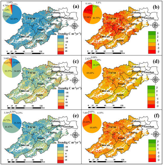
Figure 8.
Trend (a) and significance (b) of GPP, trend (c) and significance (d) of NPP, and trend (e) and significance (f) distribution of NEP of Hangzhou’s forests in the years 2001–2020.
Analyzing Figure 8a,b, it is evident that the GPP in Hangzhou forests is trending downward in the center and northwest regions while showing an upward trend in the south and northeast regions. Specifically, 8.79% of the area experienced an increasing GPP trend, with only 0.57% showing a statistically significant increase, primarily located in the northwest of Lin’an, the southwest of Jiande, and the southeast of Fuyang. Conversely, 91.21% of the area experienced a decreasing GPP trend, with 44.66% showing a statistically significant decrease, primarily concentrated in Lin’an’s western and central regions, as well as along the borders of Tonglu and Chun’an.
Analyzing Figure 8c,d, the NPP of Hangzhou forests shows an increasing trend in the southern and northeastern regions, while experiencing a decline trend in the central and northern regions. Specifically, the NPP increases by 16.72%, with a significant increase of 0.48%, mainly concentrated in the southern parts of Jiande and Fuyang, and the junction of Lin’an and Yuhang. The GPP shows a decreasing trend, with an overall decrease of 83.28%, including a significant reduction of 13.59%, primarily found at the intersection of Tonglu, Chun’an, and Lin’an.
From Figure 8e,f, it can be seen that the NEP of Hangzhou forests shows a decreasing trend in general. Only 4.23% of the NEP shows an increase, with just 0.04% showing a significant increase, primarily distributed in Jiande and the junction of Lin’an and Yuhang. In contrast, 95.77% of the NEP shows a decrease, with 31.17% of the decrease being significant, mainly in the western part of Tonglu, central and western portion of Lin’an, and the southwestern portion of Chun’an.
3.3. Influence of Phenology on the Carbon Cycle
3.3.1. Influence of Phenology on GPP
Figure 9 displays the spatial distribution of correlation coefficients, highlighting the significance of the relationships among SOS, EOS, and LOS with GPP. Figure 9a,c,e displays the spatial correlations among SOS, EOS, and LOS with GPP, while Figure 9b,d,f displays the significance test results for these correlations.
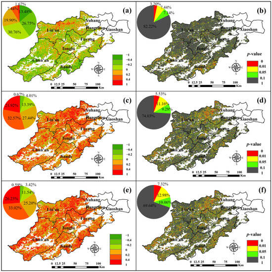
Figure 9.
Spatial distribution of correlation (a) and significance (b) of SOS and GPP, correlation (c) and significance (d) of EOS with GPP, and correlation (e) and significance (f) of LOS with GPP.
Analyzing Figure 9a,b, it can be seen that 29.01% of Hangzhou forests had correlation coefficients between SOS and GPP greater than 0, with the majority located in the northern part of Lin’an and the western area of Tonglu. However, only 1.67% of the total area had coefficients greater than 0.4, while 70.99% had coefficients less than 0. Notably, 26.75% of the area had correlation coefficients in the range of −0.2 to 0.4. This indicates that the climatic factor SOS shows an inverse relationship with GPP in most of the Hangzhou forests, suggesting that an earlier onset of the growing season positively influences GPP.
Analyzing Figure 9c,d, the correlation coefficients between EOS and GPP in Hangzhou forests were widely distributed, with 81.93% showing positive correlations. A total of 32.57% had correlation coefficients between 0.2 and 0.4, and 21.92% had correlation coefficients greater than 0.4. In contrast, 18.07% of the area had negative correlations, primarily in the northwestern part of Lin’an and the northeastern part of Chun’an, with only 0.67% having correlation values less than -0.4. This suggests that EOS and GPP are positively correlated in the majority of forest in Hangzhou, indicating that a delay in EOS positively influences GPP.
Analyzing Figure 9e,f, the correlation coefficients between LOS and GPP in Hangzhou forests were widely distributed, with 84.45% showing positive correlations. Among these, 33.02% had coefficients between 0.2 and 0.4, and 26.23% had coefficients greater than 0.4. Conversely, 15.55% had negative correlations, with only 0.59% of the area showing coefficients less than −0.4, mainly in the northwest area of Lin’an. This indicates that the majority of forests in Hangzhou have a positive relationship between LOS and GPP, suggesting that a longer growing season positively influences GPP.
3.3.2. Influence of Phenology on NPP
Figure 10 displays the spatial distribution of correlation coefficients, highlighting the significance of the relationships among SOS, EOS, and LOS with NPP. Figure 10a,c,e display how the correlations among SOS, EOS, and LOS relate to NPP spatially, while Figure 10b,d,f display the significance test results for these correlations.
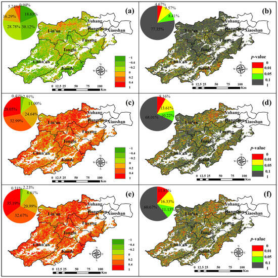
Figure 10.
Spatial distribution of correlation (a) and significance (b) of SOS and NPP, correlation (c) and significance (d) of EOS with NPP, and correlation (e) and significance (f) of LOS with NPP.
From Figure 10a,b, it can be seen that the correlation coefficients of SOS and NPP in Hangzhou forests were mostly negative, covering 77.53% of the area. These negative correlations were more uniformly distributed, with 30.12% having coefficients between −0.2 and −0.4, and 18.63% having coefficients less than −0.4. In contrast, 22.47% of the area had positive coefficients, primarily in the northern region of Lin’an, where only 0.93% of the region showed a correlation coefficient greater than 0.4. Similar to the effect of SOS on GPP, the effects of SOS and NPP are mainly negatively correlated in most forests, suggesting that an earlier SOS positively influences NPP
From Figure 10c,d, the correlation coefficients between EOS and NPP in Hangzhou forests were mostly positive, with only 14.32% showing negative correlations. The positive correlations accounted for 85.68%, widely distributed across the region. Among these, 32.99% had correlation coefficients between 0.2 and 0.4, and 28.05% had coefficients greater than 0.4. The majority of Hangzhou forests showed a positive relationship between EOS and NPP, suggesting that a delayed EOS has a beneficial impact on the increase in NPP. This effect is similar to that of SOS on GPP.
As can be seen from Figure 10e,f, it is observed that only 11.14% of Hangzhou forests showed negative correlations between LOS and NPP, with 8.61% having coefficients between −0.2 and 0. The remaining 88.86% showed positive correlations and were widely distributed across the area. Of this, 32.67% had coefficients between 0.2 and 0.4, and 35.19% had coefficients greater than 0.4. The vast majority of Hangzhou forests show a positive relationship between LOS and NPP, suggesting that the lengthening of the growing season positively influences NPP. This effect is similar to that of LOS on GPP.
3.3.3. Influence of Phenology on NEP
Figure 11 displays how correlation coefficients are spread out spatially, highlighting the significance of the relationships among SOS, EOS, and LOS with NEP. Figure 11a,c,e illustrate how the correlations among SOS, EOS, and LOS relate to NEP, while Figure 11b,d,f showcase the corresponding significance test results.
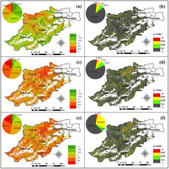
Figure 11.
Spatial distribution of correlation (a) and significance (b) of SOS and NEP, correlation (c) and significance (d) of EOS with NEP, and correlation (e) and significance (f) of LOS with NEP.
From Figure 10a,b, the correlation coefficients between SOS and NEP were negative in 62.91% of cases. Among these, 23.17% fell within the range of −0.2 to −0.4, and 9.12% were less than −0.4. Positive correlations accounted for 37.09%, primarily located in the northwestern part of Lin’an, as well as the junction of Tonglu and Chun’an, with only 2.65% having coefficients greater than 0.4. This pattern is similar to the effects of SOS on GPP and NPP, where SOS and NEP are predominantly negatively correlated, indicating that an advancement in SOS has a positive effect on the increase in NPP.
As illustrated in Figure 11c,d, the correlation coefficients between EOS and NEP in Hangzhou forests were negative for 24.43%, with 5.69% ranging from −0.2 to −0.4. Positive correlations dominate, accounting for 75.57%, and the distribution range was wide. Of these, 29.4% fell between 0.2 and 0.4, while 14.65% exceeded 0.4. This is similar to the effect of EOS on GPP and NPP. EOS and NPP are positively correlated in most forests in Hangzhou, indicating that a delayed EOS has a positive impact on the increase in NPP.
Figure 11e,f show that 23.18% of Hangzhou forests had a negative correlation coefficient between LOS and NEP. These negative correlations were primarily spread in the west of Lin’an and the northeast of Chun’an, with 16.86% falling between −0.2 and 0. Positive correlations, accounting for 76.82%, were widely distributed. Among these, 30.17% had coefficients between 0.2 and 0.4, and 16.58% is greater than 0.4. This is similar to the effect of LOS on GPP and NPP. LOS is positively correlated with NPP in most forests in Hangzhou, indicating that the lengthening of the growing season has a positive impact on NEP.
3.4. Influence of Phenology and Climate on Carbon Cycle Changes
Based on the results of phenology inversion and carbon cycle simulation, combined with meteorological data and the SEM model, the relative importance of meteorological factors such as Rad, Pre, Tmax, and Tmin and phenological factors such as SOS, EOS, and LOS on GPP were calculated.
Figure 12 illustrates the relative significance of phenological and meteorological factors on changes in the carbon cycle in the forest ecosystem of Hangzhou. As shown in Figure 12, the flux coefficients (in absolute value) of phenological and meteorological factors on GPP were ranked as follows: EOS (1.34) > Tmax (1.15) > LOS (0.64) > Pre (0.56) > Tmin (0.38) > SOS (0.18) > Rad (0.11). For NPP, the flux coefficients (in absolute value) were ordered as follows: Tmax (1.31) > EOS (1.30) > LOS (0.50) =Tmin (0.50) > Pre (0.46) > SOS (0.11) = Rad (0.11). For NEP, the pass-through coefficients (in absolute value) were ranked as follows: LOS (2.55) > SOS (1.51) > EOS (1.09) > Tmax (0.50) > EOS (0.18) > Rad (0.11) Although phenological factors are important in determining the temporal and geographical variability of carbon cycling in Hangzhou forest ecosystems, meteorological factors also have a significant impact on the carbon cycle.
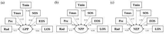
Figure 12.
The impact of phenological characteristics and climate variables on GPP (a), NPP (b), and NEP (c).
Figure 13 illustrates both the direct and indirect effects of phenology and climate change on carbon cycle changes. From Figure 13, it can be seen that the direct influence of phenological changes on carbon cycle changes was 0.85, while the direct influence of climate change on carbon cycle changes (the absolute value of the throughput coefficient) was 1.03. The direct impact of climate change on carbon cycle changes was slightly larger than that of phenological changes. Additionally, climate change can also indirectly have an influence on the carbon cycle through phenological changes, with the indirect influence of climate on the carbon cycle calculated as 0.51 (0.6 × 0.85 = 0.51).
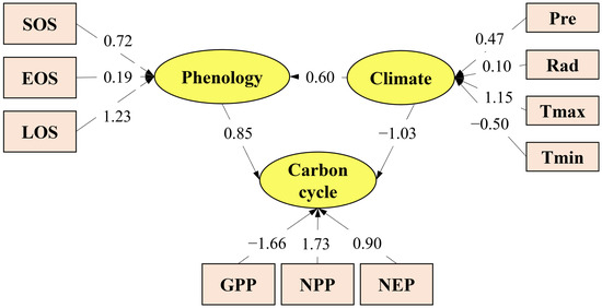
Figure 13.
Hangzhou forest ecosystems: direct and indirect effects of phenological variations and climatic change on changes in the carbon cycle, 2001–2020.
4. Discussion
In this study, we analyzed the trend of GPP, NPP, and NEP in Hangzhou’s forest ecosystems and their response to phenology. As can be seen from Figure 6, GPP, NPP, and NEP in different regions of Hangzhou showed significant spatial differences. Such differences may be closely related to the differences in regional climatic conditions. Changes in temperature and precipitation directly affect the photosynthetic efficiency of forests, which in turn affects the GPP, NPP, and NEP [61]. Our results showed that the annual averages of the indicator exhibited a declining trend (Figure 8). This decline can likely be attributed to Hangzhou’s urban expansion, which has reduced forest areas, strained land resources, and damaged farmland and natural ecosystems [62,63]. The negative effects of urbanization highlight the significant disruption of the forest carbon cycle in urban areas caused by human activities [64]. This highlights the urgent need for conservation efforts aimed at safeguarding urban forest ecosystems amid rapid urban expansion. Additionally, we found that the LOS positively influenced the increase in GPP, NPP, and NEP. This result aligns with Piao [23] and Zhao [65], which reported a similar relationship in other regions. The agreement may stem from the similarities in Hangzhou’s climatic conditions with other regions and the widespread nature of phenological patterns. With a steady increase in temperature and sunshine length at the beginning of the season, vegetation starts to recover and grow, photosynthesis starts to be active, and the rate of CO2 uptake by plants increases, and GPP increases in response [52,66]. When the season comes to an end, vegetation gradually enters dormancy, and GPP may decline [67]. It also reflects the common mechanisms through which phenological changes drive carbon cycle processes in the context of urbanization.
Compared with the common Biome-BGC and TRENDY models, the InTEC model has unique advantages. The Biome-BGC model focuses on ecosystem process simulation and is widely used in vegetation productivity and carbon flux simulation, but it has limitations in dealing with complex terrain and urban environmental heterogeneity. The TRENDY model integrates multiple dynamic global vegetation models to analyze carbon cycle at a global scale. However, the simulation accuracy of the TRENDY model at a regional scale, especially in areas affected by urbanization, needs to be improved. The InTEC model, in contrast, explicitly incorporates regional climatic characteristics and land use changes, making it particularly well suited for capturing the carbon dynamics of Hangzhou’s urban forest ecosystem. Despite these advantages, certain uncertainties remain. Model validation is a critical step, and future research should prioritize cross-verification of InTEC model outputs with field-based observations. In this study, while we standardized spatial data to a 250 m × 250 m resolution, certain datasets, such as nitrogen deposition (originally at 5° × 3.75°) and meteorological data (originally at 1000 m), required downscaling. The downscaling process may introduce uncertainties due to potential biases in interpolation techniques and the assumption that finer-scale variations follow broader spatial trends. Additionally, CO2 concentration data were obtained from global monitoring stations, which may not fully capture the fine-scale spatial heterogeneity of CO2 levels in urban areas. Beyond climatic factors, urban-induced changes such as the urban heat island (UHI) effect and land use transitions also play pivotal roles in shaping forest carbon dynamics. Elevated temperatures in urbanized areas can exacerbate climatic extremes such as heatwaves and droughts, increasing water stress and altering forest physiological processes. Studies have shown that in urbanized environments, heat island effects can advance phenological events by approximately 5 days [68], potentially influencing annual carbon uptake.
To enhance the robustness of carbon cycle modeling in urban forest ecosystems, future studies should integrate the UHI effect and dynamic land use data to provide a more comprehensive assessment of their combined impacts. Incorporating high-resolution remote sensing data and machine learning approaches could further improve model precision, enabling a deeper understanding of the interactions between urbanization and forest carbon dynamics under changing environmental conditions.
5. Conclusions
In order to simulate the carbon cycle of the Hangzhou forest ecosystem for 20 years, from 2001 to 2020, we integrated the forest phenology inversion data into the InTEC model. The key findings from the study are as follows:
(1) The spatial and temporal dynamics of GPP revealed a distinct pattern, with higher productivity in the southeast and northwest and lower productivity in the southwest. However, a consistent declining trend was observed in the annual means of GPP, NPP, and NEP across the study period, indicating a weakening carbon sink capacity.
(2) Phenological changes emerged as a critical regulator of forest carbon fluxes. Specifically, EOS enhanced GPP, NPP, and NEP, while an earlier SOS suppressed them. These relationships underscore the importance of phenological timing in governing annual carbon uptake.
(3) Structural equation modeling revealed that both climate and phenology jointly affect the carbon cycle, but through different pathways. Climate change exerted a stronger direct effect, primarily through Tmax influencing NPP. In contrast, phenology exerted a direct effect of 0.85, with EOS strongly influencing GPP and LOS being pivotal for NEP.
Overall, this study highlights that phenological shifts—often overlooked in large-scale carbon assessments—play a substantial and quantifiable role in modulating forest carbon dynamics. Our results demonstrate that incorporating phenology into ecosystem models is essential to improving the accuracy of carbon cycle simulations, particularly in the context of ongoing climate change.
Author Contributions
M.H.: Writing—original draft, Data curation, Methodology, Software, Validation, Visualization. X.L.: Writing—original draft and analysis. H.D.: Visualization and revised the manuscript. G.Z.: Visualization and revised the manuscript. F.M.: Software and analysis. Z.H.: Contributed data survey and analysis. J.X.: Contributed data survey and analysis. Y.Z.: Contributed data survey and analysis. All authors have read and agreed to the published version of the manuscript.
Funding
The research was supported by the National Natural Science Foundation of China (No. 32201553, 32171785, U1809208), the Key Research and Development Program of Zhejiang Province (Grant Nos. 2022C03039; 2021C02005).
Data Availability Statement
The original contributions presented in this study are included in the article. Further inquiries can be directed to the corresponding author.
Conflicts of Interest
The authors declare no conflict of interest.
References
- Broich, M.; Huete, A.; Tulbure, M.G.; Ma, X.; Xin, Q.; Paget, M.; Restrepo-Coupe, N.; Davies, K.; Devadas, R.; Held, A. Land Surface Phenological Response to Decadal Climate Variability across Australia Using Satellite Remote Sensing. Biogeosciences 2014, 11, 5181–5198. [Google Scholar] [CrossRef]
- Costanza, R.; d’Arge, R.; De Groot, R.; Farber, S.; Grasso, M.; Hannon, B.; Limburg, K.; Naeem, S.; O’neill, R.V.; Paruelo, J. The Value of the World’s Ecosystem Services and Natural Capital. Nature 1997, 387, 253–260. [Google Scholar] [CrossRef]
- White, M.A.; Nemani, R.R.; Thornton, P.E.; Running, S.W. Satellite Evidence of Phenological Differences between Urbanized and Rural Areas of the Eastern United States Deciduous Broadleaf Forest. Ecosystems 2002, 5, 260–273. [Google Scholar] [CrossRef]
- Ren, P.; Liu, Z.; Zhou, X.; Peng, C.; Xiao, J.; Wang, S.; Li, X.; Li, P. Strong Controls of Daily Minimum Temperature on the Autumn Photosynthetic Phenology of Subtropical Vegetation in China. For. Ecosyst. 2021, 8, 1–12. [Google Scholar] [CrossRef]
- Tang, J.; Körner, C.; Muraoka, H.; Piao, S.; Shen, M.; Thackeray, S.J.; Yang, X. Emerging Opportunities and Challenges in Phenology: A Review. Ecosphere 2016, 7, e01436. [Google Scholar] [CrossRef]
- Mascolo, L.; Martinez-Marin, T.; Lopez-Sanchez, J.M. Optimal Grid-Based Filtering for Crop Phenology Estimation with Sentinel-1 SAR Data. Remote Sens. 2021, 13, 4332. [Google Scholar] [CrossRef]
- Berra, E.F.; Gaulton, R. Remote Sensing of Temperate and Boreal Forest Phenology: A Review of Progress, Challenges and Opportunities in the Intercomparison of in-Situ and Satellite Phenological Metrics. For. Ecol. Manag. 2021, 480, 118663. [Google Scholar] [CrossRef]
- Schwartz, M.D.; Ahas, R.; Aasa, A. Onset of Spring Starting Earlier across the Northern Hemisphere. Glob. Change Biol. 2006, 12, 343–351. [Google Scholar] [CrossRef]
- Lian, X.; Piao, S.; Li, L.Z.X.; Li, Y.; Huntingford, C.; Ciais, P.; Cescatti, A.; Janssens, I.A.; Peñuelas, J.; Buermann, W. Summer Soil Drying Exacerbated by Earlier Spring Greening of Northern Vegetation. Sci. Adv. 2020, 6, eaax0255. [Google Scholar] [CrossRef]
- Xu, X.; Zhou, G.; Du, H.; Mao, F.; Xu, L.; Li, X.; Liu, L. Combined MODIS Land Surface Temperature and Greenness Data for Modeling Vegetation Phenology, Physiology, and Gross Primary Production in Terrestrial Ecosystems. Sci. Total Environ. 2020, 726, 137948. [Google Scholar] [CrossRef]
- Piao, S.; Liu, Q.; Chen, A.; Janssens, I.A.; Fu, Y.; Dai, J.; Liu, L.; Lian, X.U.; Shen, M.; Zhu, X. Plant Phenology and Global Climate Change: Current Progresses and Challenges. Glob. Change Biol. 2019, 25, 1922–1940. [Google Scholar] [CrossRef] [PubMed]
- Dragoni, D.; Schmid, H.P.; Wayson, C.A.; Potter, H.; Grimmond, C.S.B.; Randolph, J.C. Evidence of Increased Net Ecosystem Productivity Associated with a Longer Vegetated Season in a Deciduous Forest in South-Central Indiana, USA. Glob. Change Biol. 2011, 17, 886–897. [Google Scholar] [CrossRef]
- Schwartz, M.D. Phenology: An Integrative Environmental Science; Springer: Berlin/Heidelberg, Germany, 2003; Volume 132. [Google Scholar]
- Richardson, A.D.; Andy Black, T.; Ciais, P.; Delbart, N.; Friedl, M.A.; Gobron, N.; Hollinger, D.Y.; Kutsch, W.L.; Longdoz, B.; Luyssaert, S. Influence of Spring and Autumn Phenological Transitions on Forest Ecosystem Productivity. Philos. Trans. R. Soc. B Biol. Sci. 2010, 365, 3227–3246. [Google Scholar] [CrossRef]
- Li, X.; Du, H.; Zhou, G.; Mao, F.; Zheng, J.; Liu, H.; Huang, Z.; He, S. Spatiotemporal Dynamics in Assimilated-LAI Phenology and Its Impact on Subtropical Bamboo Forest Productivity. Int. J. Appl. Earth Obs. Geoinf. 2021, 96, 102267. [Google Scholar] [CrossRef]
- Han, Q.; Wang, T.; Jiang, Y.; Fischer, R.; Li, C. Phenological Variation Decreased Carbon Uptake in European Forests during 1999–2013. For. Ecol. Manag. 2018, 427, 45–51. [Google Scholar] [CrossRef]
- Black, T.A.; Chen, W.J.; Barr, A.G.; Arain, M.A.; Chen, Z.; Nesic, Z.; Hogg, E.H.; Neumann, H.H.; Yang, P.C. Increased Carbon Sequestration by a Boreal Deciduous Forest in Years with a Warm Spring. Geophys. Res. Lett. 2000, 27, 1271–1274. [Google Scholar] [CrossRef]
- Chen, J.; Chen, W.; Liu, J.; Cihlar, J.; Gray, S. Annual Carbon Balance of Canada’s Forests during 1895–1996. Glob. Biogeochem. Cycles 2000, 14, 839–849. [Google Scholar] [CrossRef]
- Xiao, J.; Chevallier, F.; Gomez, C.; Guanter, L.; Hicke, J.A.; Huete, A.R.; Ichii, K.; Ni, W.; Pang, Y.; Rahman, A.F. Remote Sensing of the Terrestrial Carbon Cycle: A Review of Advances over 50 Years. Remote Sens. Environ. 2019, 233, 111383. [Google Scholar] [CrossRef]
- Chapin, F.S.; Woodwell, G.M.; Randerson, J.T.; Rastetter, E.B.; Lovett, G.M.; Baldocchi, D.D.; Clark, D.A.; Harmon, M.E.; Schimel, D.S.; Valentini, R. Reconciling Carbon-Cycle Concepts, Terminology, and Methods. Ecosystems 2006, 9, 1041–1050. [Google Scholar] [CrossRef]
- Wang, Z.; He, Y.; Niu, B.; Wu, J.; Zhang, X.; Zu, J.; Huang, K.; Li, M.; Cao, Y.; Zhang, Y. Sensitivity of Terrestrial Carbon Cycle to Changes in Precipitation Regimes. Ecol. Indic. 2020, 113, 106223. [Google Scholar] [CrossRef]
- Keenan, T.F.; Gray, J.; Friedl, M.A.; Toomey, M.; Bohrer, G.; Hollinger, D.Y.; Munger, J.W.; O’Keefe, J.; Schmid, H.P.; Wing, I.S. Net Carbon Uptake Has Increased through Warming-Induced Changes in Temperate Forest Phenology. Nat. Clim. Chang. 2014, 4, 598–604. [Google Scholar] [CrossRef]
- Piao, S.; Friedlingstein, P.; Ciais, P.; Viovy, N.; Demarty, J. Growing Season Extension and Its Impact on Terrestrial Carbon Cycle in the Northern Hemisphere over the Past 2 Decades. Glob. Biogeochem. Cycles 2007, 21. [Google Scholar] [CrossRef]
- Cramer, W.; Bondeau, A.; Schaphoff, S.; Lucht, W.; Smith, B.; Sitch, S. Tropical Forests and the Global Carbon Cycle: Impacts of Atmospheric Carbon Dioxide, Climate Change and Rate of Deforestation. Philos. Trans. R. Soc. London. Ser. B Biol. Sci. 2004, 359, 331–343. [Google Scholar] [CrossRef] [PubMed]
- Houghton, R.A. Interactions between Land-Use Change and Climate-Carbon Cycle Feedbacks. Curr. Clim. Chang. Rep. 2018, 4, 115–127. [Google Scholar] [CrossRef]
- Li, Y.; Brando, P.M.; Morton, D.C.; Lawrence, D.M.; Yang, H.; Randerson, J.T. Deforestation-Induced Climate Change Reduces Carbon Storage in Remaining Tropical Forests. Nat. Commun. 2022, 13, 1964. [Google Scholar] [CrossRef]
- Huang, C.; Weishu, G.; Yong, P. Remote Sensing and Forest Carbon Monitoring--a Review of Recent Progress, Challenges and Opportunities. J. Geod. Geoinf. Sci. 2022, 5, 124. [Google Scholar]
- Turner, D.P.; Guzy, M.; Lefsky, M.A.; Ritts, W.D.; Van Tuyl, S.; Law, B.E. Monitoring Forest Carbon Sequestration with Remote Sensing and Carbon Cycle Modeling. Environ. Manag. 2004, 33, 457–466. [Google Scholar] [CrossRef]
- Xie, X.; Li, A.; Jin, H. The Simulation Models of the Forest Carbon Cycle on a Large Scale: A Review. Acta Ecol. Sin. 2018, 38, 41–54. [Google Scholar]
- Zheng, J.; Mao, F.; Du, H.; Li, X.; Zhou, G.; Dong, L.; Zhang, M.; Han, N.; Liu, T.; Xing, L. Spatiotemporal Simulation of Net Ecosystem Productivity and Its Response to Climate Change in Subtropical Forests. Forests 2019, 10, 708. [Google Scholar] [CrossRef]
- Zhang, F.; Chen, J.M.; Pan, Y.; Birdsey, R.A.; Shen, S.; Ju, W.; He, L. Attributing Carbon Changes in Conterminous US Forests to Disturbance and Non-disturbance Factors from 1901 to 2010. J. Geophys. Res. Biogeosci. 2012, 117. [Google Scholar]
- He, L.; Chen, J.M.; Pan, Y.; Birdsey, R.; Kattge, J. Relationships between Net Primary Productivity and Forest Stand Age in US Forests. Glob. Biogeochem. Cycles 2012, 26. [Google Scholar] [CrossRef]
- Govind, A.; Chen, J.M.; Bernier, P.; Margolis, H.; Guindon, L.; Beaudoin, A. Spatially Distributed Modeling of the Long-Term Carbon Balance of a Boreal Landscape. Ecol. Model. 2011, 222, 2780–2795. [Google Scholar] [CrossRef]
- Hu, M.; Li, X.; Xu, Y.; Huang, Z.; Chen, C.; Chen, J.; Du, H. Remote Sensing Monitoring of the Spatiotemporal Dynamics of Urban Forest Phenology and Its Response to Climate and Urbanization. Urban Clim. 2024, 53, 101810. [Google Scholar] [CrossRef]
- Cao, B.; Gruber, S.; Zhang, T. REDCAPP (v1. 0): Parameterizing Valley Inversions in Air Temperature Data Downscaled from Reanalyses. Geosci. Model Dev. 2017, 10, 2905–2923. [Google Scholar] [CrossRef]
- Ju, W.; Chen, J.M.; Black, T.A.; Barr, A.G.; Liu, J.; Chen, B. Modelling Multi-Year Coupled Carbon and Water Fluxes in a Boreal Aspen Forest. Agric. For. Meteorol. 2006, 140, 136–151. [Google Scholar] [CrossRef]
- Guber, A.K.; Pachepsky, Y.A.; Van Genuchten, M.T.; Rawls, W.J.; Simunek, J.; Jacques, D.; Nicholson, T.J.; Cady, R.E. Field-Scale Water Flow Simulations Using Ensembles of Pedotransfer Functions for Soil Water Retention. Vadose Zone J. 2006, 5, 234–247. [Google Scholar] [CrossRef]
- Koren, V.; Smith, M.; Duan, Q. Use of a Priori Parameter Estimates in the Derivation of Spatially Consistent Parameter Sets of Rainfall-Runoff Models. Calibration Watershed Models 2003, 6, 239–254. [Google Scholar]
- Yang, J.; Huang, X. The 30 m Annual Land Cover Dataset and Its Dynamics in China from 1990 to 2019. Earth Syst. Sci. Data 2021, 13, 3907–3925. [Google Scholar] [CrossRef]
- Li, L.; Lu, D.; Kuang, W. Examining Urban Impervious Surface Distribution and Its Dynamic Change in Hangzhou Metropolis. Remote Sens. 2016, 8, 265. [Google Scholar] [CrossRef]
- Li, X.; Du, H.; Mao, F.; Zhou, G.; Chen, L.; Xing, L.; Fan, W.; Xu, X.; Liu, Y.; Cui, L. Estimating Bamboo Forest Aboveground Biomass Using EnKF-Assimilated MODIS LAI Spatiotemporal Data and Machine Learning Algorithms. Agric. For. Meteorol. 2018, 256, 445–457. [Google Scholar] [CrossRef]
- Mao, F.; Du, H.; Zhou, G.; Li, X.; Xu, X.; Li, P.; Sun, S. Coupled LAI Assimilation and BEPS Model for Analyzing the Spatiotemporal Pattern and Heterogeneity of Carbon Fluxes of the Bamboo Forest in Zhejiang Province, China. Agric. For. Meteorol. 2017, 242, 96–108. [Google Scholar] [CrossRef]
- Sen, P.K. Estimates of the Regression Coefficient Based on Kendall’s Tau. J. Am. Stat. Assoc. 1968, 63, 1379–1389. [Google Scholar] [CrossRef]
- Theil, H. A Rank-Invariant Method of Linear and Polynomial Regression Analysis. Indag. Math. 1950, 12, 173. [Google Scholar]
- Liu, H.; Liu, S.; Wang, F.; Liu, Y.; Yu, L.; Wang, Q.; Sun, Y.; Li, M.; Sun, J.; Han, Z. Management Practices Should Be Strengthened in High Potential Vegetation Productivity Areas Based on Vegetation Phenology Assessment on the Qinghai-Tibet Plateau. Ecol. Indic. 2022, 140, 108991. [Google Scholar] [CrossRef]
- Zhang, R.; Qi, J.; Leng, S.; Wang, Q. Long-Term Vegetation Phenology Changes and Responses to Preseason Temperature and Precipitation in Northern China. Remote Sens. 2022, 14, 1396. [Google Scholar] [CrossRef]
- Parmesan, C. Influences of Species, Latitudes and Methodologies on Estimates of Phenological Response to Global Warming. Glob. Change Biol. 2007, 13, 1860–1872. [Google Scholar] [CrossRef]
- Shang, L.; Liao, J.; Xie, S.; Tu, Z.; Liao, H.; Zhong, K. Dynamic Changes in the Thermal Growing Season and Their Association with Atmospheric Circulation in China. Int. J. Biometeorol. 2022, 66, 545–558. [Google Scholar] [CrossRef] [PubMed]
- Hamed, K.H. Trend Detection in Hydrologic Data: The Mann–Kendall Trend Test under the Scaling Hypothesis. J. Hydrol. 2008, 349, 350–363. [Google Scholar] [CrossRef]
- Kendall, M.G. Rank Correlation Methods; Springer: Berlin/Heidelberg, Germany, 1948. [Google Scholar]
- Liu, J.; Zhan, P. The Impacts of Smoothing Methods for Time-Series Remote Sensing Data on Crop Phenology Extraction. In Proceedings of the 2016 IEEE International Geoscience and Remote Sensing Symposium (IGARSS), Beijing, China, 10–15 July 2016; pp. 2296–2299. [Google Scholar]
- Chen, W.; Chen, J.; Cihlar, J. An Integrated Terrestrial Ecosystem Carbon-Budget Model Based on Changes in Disturbance, Climate, and Atmospheric Chemistry. Ecol. Model. 2000, 135, 55–79. [Google Scholar] [CrossRef]
- Chen, W.; Chen, J.; Liu, J.; Cihlar, J. Approaches for Reducing Uncertainties in Regional Forest Carbon Balance. Glob. Biogeochem. Cycles 2000, 14, 827–838. [Google Scholar] [CrossRef]
- Wang, B.; Li, M.; Fan, W.; Yu, Y.; Chen, J.M. Relationship between Net Primary Productivity and Forest Stand Age under Different Site Conditions and Its Implications for Regional Carbon Cycle Study. Forests 2018, 9, 5. [Google Scholar] [CrossRef]
- Wang, S.; Chen, J.M.; Ju, W.M.; Feng, X.; Chen, M.; Chen, P.; Yu, G. Carbon Sinks and Sources in China’s Forests during 1901–2001. J. Environ. Manag. 2007, 85, 524–537. [Google Scholar] [CrossRef] [PubMed]
- Li, X.; Mao, F.; Du, H.; Zhou, G.; Xu, X.; Li, P.; Liu, Y.; Cui, L. Simulating of Carbon Fluxes in Bamboo Forest Ecosystem Using BEPS Model Based on the LAI Assimilated with Dual Ensemble Kalman Filter. Chin. J. Appl. Ecol. 2016, 27, 3797–3806. [Google Scholar]
- Li, X.; Mao, F.; Du, H.; Zhou, G.; Xu, X.; Han, N.; Sun, S.; Gao, G.; Chen, L. Assimilating Leaf Area Index of Three Typical Types of Subtropical Forest in China from MODIS Time Series Data Based on the Integrated Ensemble Kalman Filter and PROSAIL Model. ISPRS J. Photogramm. Remote Sens. 2017, 126, 68–78. [Google Scholar] [CrossRef]
- Ge, H.; Zhou, G.; Liu, E.; Liu, A.; Ye, G. Diameter-Age Bivariate Weibull Distribution Model for Moso Bamboo Forests in Zhejiang Province. Sci. Silvae Sin. 2008, 44, 15–20. [Google Scholar]
- Jeuken, A.; Veefkind, J.P.; Dentener, F.; Metzger, S.; Gonzalez, C.R. Simulation of the Aerosol Optical Depth over Europe for August 1997 and a Comparison with Observations. J. Geophys. Res. Atmos. 2001, 106, 28295–28311. [Google Scholar] [CrossRef]
- Lelieveld, J.; Dentener, F.J. What Controls Tropospheric Ozone? J. Geophys. Res. Atmos. 2000, 105, 3531–3551. [Google Scholar] [CrossRef]
- Collalti, A.; Ibrom, A.; Stockmarr, A.; Cescatti, A.; Alkama, R.; Fernández-Martínez, M.; Matteucci, G.; Sitch, S.; Friedlingstein, P.; Ciais, P. Forest Production Efficiency Increases with Growth Temperature. Nat. Commun. 2020, 11, 5322. [Google Scholar] [CrossRef]
- Cumming, G.S.; Buerkert, A.; Hoffmann, E.M.; Schlecht, E.; von Cramon-Taubadel, S.; Tscharntke, T. Implications of Agricultural Transitions and Urbanization for Ecosystem Services. Nature 2014, 515, 50–57. [Google Scholar] [CrossRef]
- Li, R.-Q.; Dong, M.; Cui, J.-Y.; Zhang, L.-L.; Cui, Q.-G.; He, W.-M. Quantification of the Impact of Land-Use Changes on Ecosystem Services: A Case Study in Pingbian County, China. Environ. Monit. Assess. 2007, 128, 503–510. [Google Scholar] [CrossRef]
- Wu, Y.; Yang, J.; Li, S.; Zhao, Y.; Guo, C.; Yang, X.; Xu, Y.; Yue, F.; Zhang, Z.; Yang, S. Decoding Carbon Pathways of Shanghai Megacity through Historical Land Use Patterns and Urban Ecosystem Transitions. Sci. Rep. 2025, 15, 6326. [Google Scholar] [CrossRef] [PubMed]
- Zhao, J.; Liu, L. Effects of Phenological Change on Ecosystem Productivity of Temperate Deciduous Broadleaved Forests in North America. Chin. J. Plant Ecol. 2012, 36, 363–371. [Google Scholar] [CrossRef]
- Wu, C.; Chen, J.M.; Gonsamo, A.; Price, D.T.; Black, T.A.; Kurz, W.A. Interannual Variability of Carbon Sequestration Is Determined by the Lag between Ends of Net Uptake and Photosynthesis: Evidence from Long Records of Two Contrasting Forest Stands. Agric. For. Meteorol. 2012, 164, 29–38. [Google Scholar] [CrossRef]
- Coursolle, C.; Margolis, H.A.; Barr, A.G.; Black, T.A.; Amiro, B.D.; McCaughey, J.H.; Flanagan, L.B.; Lafleur, P.M.; Roulet, N.T.; Bourque, C.P.-A. Late-Summer Carbon Fluxes from Canadian Forests and Peatlands along an East West Continental Transect. Can. J. For. Res. 2006, 36, 783–800. [Google Scholar] [CrossRef]
- Zipper, S.C.; Schatz, J.; Singh, A.; Kucharik, C.J.; Townsend, P.A.; Loheide, S.P. Urban Heat Island Impacts on Plant Phenology: Intra-Urban Variability and Response to Land Cover. Environ. Res. Lett. 2016, 11, 54023. [Google Scholar] [CrossRef]
Disclaimer/Publisher’s Note: The statements, opinions and data contained in all publications are solely those of the individual author(s) and contributor(s) and not of MDPI and/or the editor(s). MDPI and/or the editor(s) disclaim responsibility for any injury to people or property resulting from any ideas, methods, instructions or products referred to in the content. |
© 2025 by the authors. Licensee MDPI, Basel, Switzerland. This article is an open access article distributed under the terms and conditions of the Creative Commons Attribution (CC BY) license (https://creativecommons.org/licenses/by/4.0/).