An Enhanced Algorithm Based on Dual-Input Feature Fusion ShuffleNet for Synthetic Aperture Radar Operating Mode Recognition

Abstract

Synthetic aperture radar (SAR) operating mode recognition plays a crucial role in SAR countermeasures and serves as the foundation for effective SAR interference. To address the limitations of current SAR operating mode recognition algorithms, such as low recognition rates, poor generalization, and limited engineering applicability under low signal-to-noise ratio (SNR) conditions, an enhanced algorithm named dual-input feature fusion ShuffleNet (DIFF-ShuffleNet) based on intercepted SAR signal data is proposed. First, the SAR signal is processed by combining pulse compression and time–frequency analysis technology to enhance anti-noise robustness. Then, an improved lightweight ShuffleNet architecture is designed to fuse range pulse compression (RPC) maps and azimuth time–frequency features, significantly improving recognition accuracy in low-SNR environments while maintaining practical deployability. Moreover, an improved coarse-to-fine search fractional Fourier transform (CFS-FRFT) algorithm is proposed to address the chirp rate estimation required for RPC. Simulations demonstrate that the proposed SAR operating mode recognition algorithm achieves over 95.00% recognition accuracy for SAR operating modes (stripmap, spotlight, sliding spotlight, and scan) at an SNR greater than −8 dB. Finally, four sets of measured SAR data are used to validate the algorithm’s effectiveness, with all recognition results being correct, demonstrating the algorithm’s practical applicability.

1. Introduction

Synthetic aperture radar (SAR) is an active imaging radar system utilizing electromagnetic waves with characteristics of high resolution, all-day, and all-weather capabilities. It is proficient in detecting camouflage and hidden bunkers, making it widely applicable in both military and civilian sectors [1,2]. The importance of anti-SAR surveillance for safeguarding critical targets and areas underscores its research significance. Moreover, SAR jamming technology has emerged as a focal point in electronic countermeasures research [3,4,5,6]. SAR employs diverse operating modes for various applications, each necessitating distinct interference techniques. Therefore, recognizing specific SAR operating modes is fundamental for successful interference strategies.

The recognition of SAR operating modes primarily involves analyzing the signals transmitted by reconnaissance SAR platforms to infer their operating modes. Currently, algorithms for SAR operating mode identification can be broadly classified into three categories: reconnaissance power analysis, intra-pulse parameter analysis, and inter-pulse parameter analysis. Liu H. et al. [7], analyzed the distinctions among strip, spotlight, and sliding spotlight SAR operating modes from various perspectives such as azimuth–frequency history, range migration, and antenna scanning speed, laying a foundation for SAR operating mode recognition. In 2012, Chen Y. et al. studied the side-lobe reconnaissance [8] and pulse repetition frequency (PRF) [9] optimization selection of SAR spotlight and sliding spotlight modes. Their findings revealed that, compared to the spotlight mode, the sliding spotlight mode exhibits lower power values and reduced antenna side-lobe gains as detected by reconnaissance receivers. Additionally, the PRF value of the sliding spotlight mode is closer to that of the strip mode. Chen Y. et al. [10] further emphasized the significant differences in antenna gain, power, and power density between strip and spotlight modes, which can serve as discriminative features for recognizing SAR operating modes; while the aforementioned studies conducted simulation analyses on power, antenna gain, and azimuth-frequency history of various SAR operating modes, they did not provide specific methods for SAR operating mode recognition.

Tang X. et al. proposed an algorithm to differentiate stripmap mode and spotlight mode, which employed the sum of squared errors between the theoretically received power arrays of the spaceborne SAR search domain and the actual received power arrays at ground receiving stations [11,12]. However, this algorithm necessitates prior knowledge of the satellite’s orbit and imposes specific requirements on the layout of reconnaissance receivers, posing challenges for non-cooperative SAR operating mode recognition. In [13], a multi-station reconnaissance approach was employed to estimate the Doppler centroid frequency of the intercepted signals using techniques such as autocorrelation, cross-correlation, and Wigner–Ville distribution. By comparing the Doppler centroid frequency values observed at different stations, the SAR operating mode can be determined. However, this algorithm can only identify whether the mode is stripmap mode and multi-station reconnaissance significantly increases the costs. Reference [14] employed the fractional Fourier transform (FRFT) combined with the minimum entropy algorithm to estimate azimuthal power. Then, Radon transform-derived Doppler parameters were utilized to assist in distinguishing between stripmap, spotlight, and sliding spotlight modes. However, the algorithm requires significant computational resources for range compression and adaptive range cell migration correction. Additionally, its reliance on manually extracted features limits its adaptability to a broader range of operating modes. In 2022, Ref. [15] proposed a SAR operating mode recognition algorithm based on the peak amplitude sequence of intercepted signals combined with a one-dimensional convolutional neural network (CNN). They introduced another algorithm in the same year that utilizes pulse peak I/Q data of reconnaissance signals in conjunction with a CGRU neural network and support vector machine (SVM) classifier [16]. Both algorithms can identify stripmap, spotlight, sliding spotlight, and scan modes, with average recognition rates exceeding 91%. However, neither algorithm accounted for low SNR, and thus they lack adaptability for complex electromagnetic environments in practical applications. In [17], a recognition algorithm based on side-lobe reconnaissance combined with a back-propagation (BP) neural network was proposed. Experimental results demonstrate that, when the SNR exceeds 0 dB, the algorithm achieves a recognition rate of over 91.67%; while this algorithm can accommodate low SNR, it does not consider the recognition of the sliding spotlight mode. Moreover, the fixed structure of the BP neural network is prone to local optima and overfitting, resulting in limited accuracy and poor generalization capability of the recognition model.

To address the problems mentioned above, this manuscript proposes a SAR operating mode recognition algorithm based on a Dual-Input Feature Fusion ShuffleNet (DIFF-ShuffleNet). Initially, the reconnaissance signals of four typical SAR operational modes (stripmap, spotlight, sliding spotlight, and scan) are modeled and simulated. To improve noise resistance, the range pulse compression (RPC) amplitude maps and azimuth time–frequency maps are introduced as neural network inputs for the first time. To further improve the algorithm’s recognition rate, a ShuffleNet structure capable of autonomously adjusting the weights of dual-input features is proposed. Addressing the issue of estimating chirp rate for range compression, an enhanced coarse-to-fine search fractional Fourier transform (CFS-FRFT) algorithm is suggested, which offers strong noise resistance and high estimation accuracy while increasing computational speed. Moreover, this manuscript analyzes the impact of the number of pulses on the algorithm’s recognition rate and applies the proposed algorithm to identify actual measured SAR reconnaissance data.

The structure of this manuscript is outlined as follows. Section 2 simulates reconnaissance signals under different SAR operating modes, drawing the conclusion that the amplitude image features of the reconnaissance signals are susceptible to noise. Section 3 provides detailed simulations and explanations for each step of the proposed algorithm. Section 4 compares the performance of the proposed algorithm with those of other existing methods and discusses the impact of the number of intercepted signal pulses on the algorithm’s performance. Moreover, the proposed algorithm is applied to process actual SAR data. Finally, Section 5 concludes the manuscript.

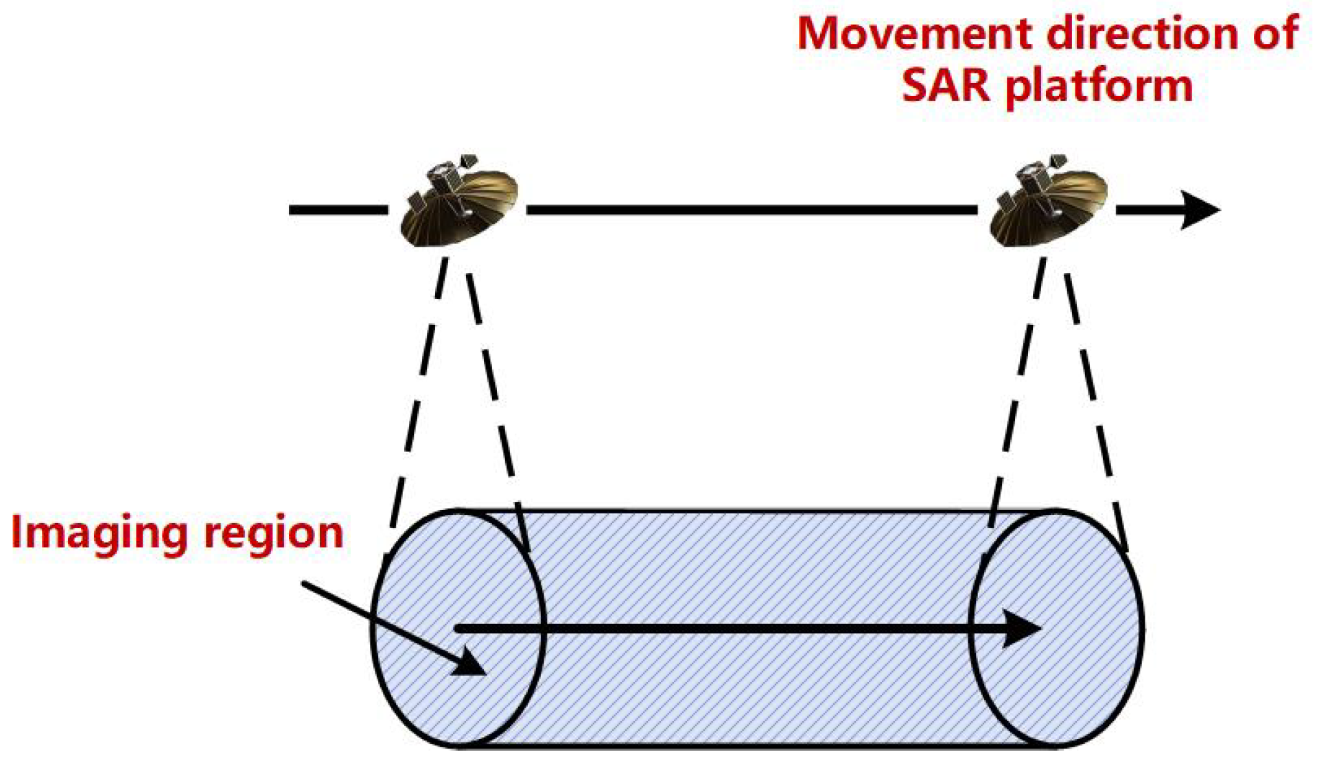
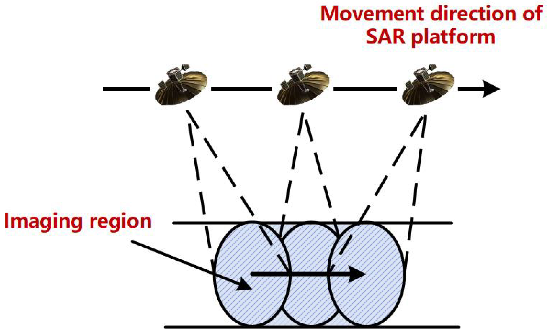
2. Modeling and Simulation of Intercepted SAR Signals Under Different Operating Modes

2.1. Modeling of the Intercepted SAR Signals

When SAR operates in different modes, there are significant variations in its imaging algorithms, processing methods, and signal parameters. These differences lead to distinct sensitivities to key parameters, necessitating tailored electronic warfare or jamming strategies. SAR has four classic operating modes: stripmap, spotlight, sliding spotlight, and scan. Each mode results in unique characteristics in the SAR signals intercepted by reconnaissance receivers.

(1) Stripmap Mode

The Stripmap mode is the most-used operating mode in SAR. In this mode, the antenna remains fixed, ensuring that parameters such as the beam’s depression angle, squint angle, and beam width remain constant during operation. As the SAR platform moves, the beam forms a strip-like mapping swath over the observation area, hence the name “stripmap mode” [18]. The schematic of this mode is illustrated in Figure 1.

According to the principle of stripmap operating mode, the expression of SAR signal received by the reconnaissance receiver is:

$$s_{\mathrm{SM}}(\tau ,t)={\omega }_a(t-t_c)\mathrm{rect}\left({\displaystyle \frac{\tau -\frac{R\left(t\right)}{c}}{T_p}}\right)exp(-j\pi {\displaystyle \frac{2R\left(t\right)}{\lambda }})exp\left[j\pi K_r{(\tau -{\displaystyle \frac{R\left(t\right)}{c}})}^2\right]$$

(1)

where $\tau$ represents the fast time in the range direction, t denotes the slow time in the azimuth direction, $w_a(·)$ is the azimuth antenna beam pattern, $\mathrm{rect}(·)$ denotes the rectangular window function, $R\left(t\right)$ is the instantaneous slant range, $T_p$ is the pulse width of the range signal, $\lambda$ is the wavelength of the transmitted signal, c is the speed of light, and $t_c$ is the azimuth centroid moment of the SAR.

(2) Spotlight Mode

In spotlight mode, SAR achieves high resolution by steering the beam to illuminate a target for an extended period. This mode significantly enhances the azimuth resolution of SAR. However, due to the extended target illumination period, the observation area becomes limited [19]. Consequently, SAR in spotlight mode trades off coverage area for enhanced resolution, as depicted in the operational schematic shown in Figure 2.

According to the principle of spotlight operating mode, the expression of SAR signal received by the reconnaissance receiver is:

$$s_{\mathrm{SL}}(\tau ,t)={\omega }_a(t-t_c)\mathrm{rect}\left({\displaystyle \frac{t-t_c}{T_{spot}}}\right)rect\left({\displaystyle \frac{t-\frac{R\left(t\right)}{c}}{T_p}}\right)exp(-j\pi {\displaystyle \frac{2R\left(t\right)}{\lambda }})exp\left[j\pi K_r{(\tau -{\displaystyle \frac{R\left(t\right)}{c}})}^2\right]$$

(2)

where $T_{spot}$ is the synthesized aperture time. The rest of the parameters are the same as in the expression for the stripmap SAR signal.

(3) Sliding Spotlight Mode

The sliding spotlight mode has been introduced to address the trade-off between high resolution and wide-area imaging encountered in strip and spotlight modes, requiring a practical compromise for effective application [20]. In this mode, the beam’s aiming point is directed downward toward the illuminated area, while the radar beam moves along the azimuth direction of the ground imaging region at a speed slower than the radar platform’s azimuthal motion. A schematic of its operation is provided in Figure 3.

According to the principle of sliding spotlight operating mode, the expression of SAR signal received by the reconnaissance receiver is:

$$s_{\mathrm{SSL}}(\tau ,t)={\omega }_a(t-t_c)\mathrm{rect}\left({\displaystyle \frac{\tau -\frac{R\left(t\right)}{c}}{T_p}}\right)\mathrm{rect}\left({\displaystyle \frac{{\nu }_{f}t-x_0}{X}}\right)exp(-j\pi {\displaystyle \frac{2R\left(t\right)}{\lambda }})exp\left[j\pi K_r{(\tau -{\displaystyle \frac{R\left(t\right)}{c}})}^2\right]$$

(3)

where $V_f$ represents the moving speed of the antenna beam center’s projection point within the scene, X denotes the projected length of the beam footprint, and $x_0$ is the azimuth coordinate of the point target. The remaining parameters are consistent with those in the expression for the stripmap SAR-detected signal.

(4) Scan Mode

Scan SAR is a crucial mode for wide-swath observation in spaceborne SAR systems. It achieves extensive coverage by rapidly switching the antenna beam among multiple sub-swaths, thereby expanding the observation width during a single satellite pass over the target area [21,22,23]. Compared to stripmap mode, scan SAR offers lower resolution but significantly wider swath coverage. A schematic of its operation is illustrated in Figure 4.

According to the principle of scan operating mode, then the expression of the detected signal in the same sub-band is as follows:

$$s_{\mathrm{Scan}}(\tau ,t)=\sum _{n=1}^N\mathrm{rect}\left({\displaystyle \frac{t-n{T}_r}{T_b}}\right){\omega }_a(t-t_c)\mathrm{rect}\left({\displaystyle \frac{t-\frac{R\left(t\right)}{c}}{T_p}}\right)exp(-j\pi {\displaystyle \frac{2R\left(t\right)}{\lambda }})exp\left[j\pi K_r{(\tau -{\displaystyle \frac{R\left(t\right)}{c}})}^2\right]$$

(4)

where $T_r$ represents the time interval between two successive imaging sessions of a sub-band, denoted as the regression time. $T_b$ corresponds to the duration of a single burst of consecutive imaging sessions within a sub-band, referred to as the dwell time, while $N_a$ signifies the azimuth multi-view number.

A comparison of the SAR signal expressions received by reconnaissance receivers in stripmap and scan modes reveals that, in scan mode, the SAR signal within the same sub-band is equivalent to the stripmap mode SAR signal subjected to window truncation. The time interval between two adjacent windows corresponds to the regression time. Consequently, the received power variation in scan mode is analogous to that in stripmap mode, with the addition of window truncation effects. When comparing the signal expressions for stripmap and spotlight modes, due to antenna rotation, the received power over the entire synthetic aperture time in spotlight mode is uniformly weighted by the antenna pattern. As a result, the received power varies solely with changes in slant range, leading to slower power fluctuations. In sliding spotlight mode, the received power variation lies between that of stripmap and spotlight modes, with the degree of change determined by the ratio of the beam scanning speed to the platform speed.

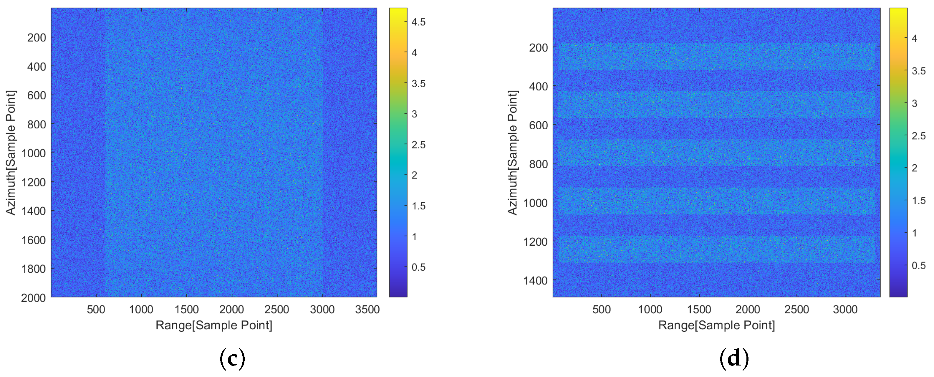
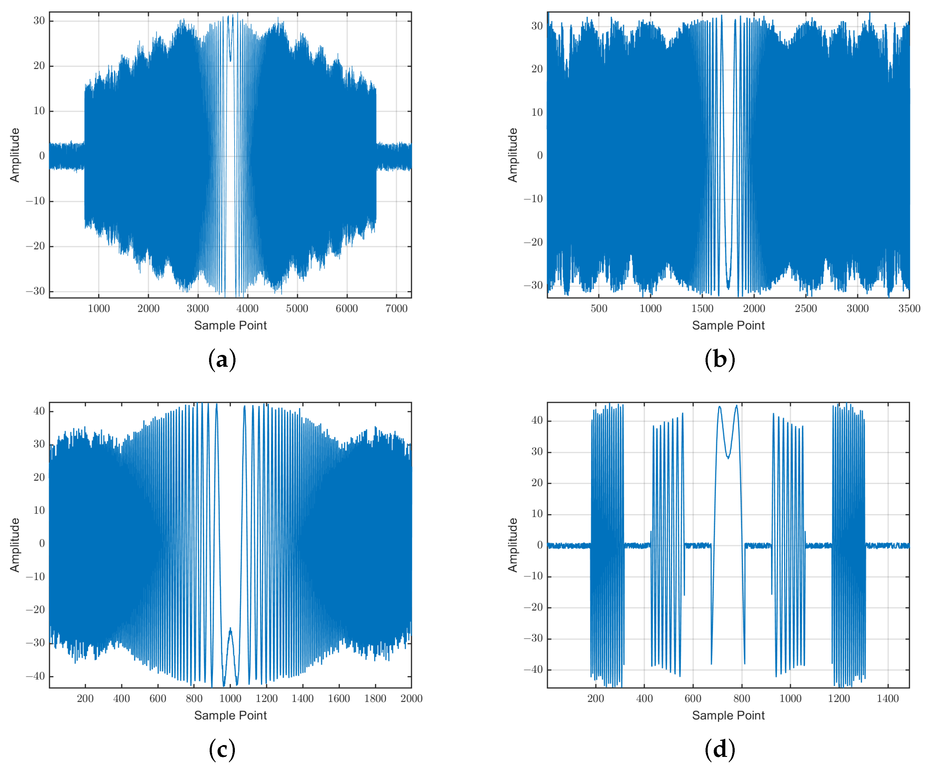
2.2. Simulation of the Intercepted Signals

To more intuitively observe the amplitude differences in detected signals across different modes, the intercepted signals under four modes are simulated. Given that linear frequency modulation (LFM) signals are the most widely used modulation type in SAR, the range signals employed in the simulation are LFM signals. The key simulation parameters are listed in

Table 1. Detecting signal parameters in different SAR operating modes.

Stripmap SAR
Carrier frequency	9.6 GHz	Slant range of scene center	600 km
Velocity of SAR platform in motion	7000 m/s	Azimuth resolution	1.14
Range signal pulse width	10 $\mathsf{\mu }$s	Range signal bandwidth	100 MHz
Range sampling frequency	150 MHz	PRF	5000.00 Hz
Spotlight SAR
Carrier frequency	9.6 GHz	Slant range of scene center	600 km
Velocity of SAR platform in motion	7000 m/s	Antenna length	6.0 m
Range signal pulse width	10 $\mathsf{\mu }$s	Range signal bandwidth	100 MHz
Range sampling frequency	150 MHz	PRF	3500 Hz
Sliding Spotlight SAR
Carrier frequency	9.6 GHz	Height of SAR platform	600 km
Velocity of SAR platform in motion	7500 m/s	Antenna length	4.8 m
Range signal pulse width	20 $\mathsf{\mu }$s	Range signal bandwidth	90 MHz
Range sampling frequency	120 MHz	PRF	3500 Hz
Scan SAR
Carrier frequency	5.3 GHz	Height of SAR platform	800 km
Velocity of SAR platform in motion	7500 m/s	Azimuth resolution	1.14
Range signal pulse width	20 $\mathsf{\mu }$s	Range signal bandwidth	100 MHz
Range sampling frequency	150 MHz	PRF	2100 Hz
Revisit time (the number of sub-bands is 5)	120 ms	Dwell time	66.75 ms

, and the two-dimensional amplitude diagrams of the detected signals for each mode are presented in Figure 5.

Figure 5 illustrates that the amplitude of the intercepted signal in stripmap mode exhibits significant variation, initially increasing and then decreasing in the azimuth direction. In contrast, the amplitude in spotlight mode remains relatively constant. The sliding spotlight mode also shows an initial increase followed by a decrease in azimuth amplitude, but the change occurs more gradually. The scan mode displays discontinuous azimuth amplitude. The two-dimensional amplitude map of the intercepted signal effectively reflects the azimuth power variation, with distinct characteristics for each mode, making it a useful tool for discriminating operating modes. However, at low SNR, these characteristic features are obscured by noise, complicating mode identification. Figure 6 demonstrates the amplitude maps for each mode at an SNR of 0 dB, where the azimuth amplitude variations become indistinct, particularly in stripmap, spotlight, and sliding spotlight modes.

3. The Proposed Algorithm

The proposed SAR operating mode recognition algorithm based on DIFF-ShuffleNet comprises two main components: the simulation data training and the actual SAR data processing. In the simulation data training part, SAR intercepted signals for four different operating modes are simulated to generate training data. For the first time, the RPC map and azimuth time–frequency map of the intercepted signals, derived from pulse compression and time–frequency analysis techniques, are utilized as feature inputs for the four operating modes. The azimuth time–frequency analysis is achieved by short-time Fourier transform (STFT) [24]. Then, a large dataset is created by randomly varying the azimuthal position of the reconnaissance platform, and the proposed DIFF-ShuffleNet is employed to train the model, resulting in a SAR operating mode recognition model. In the actual SAR data processing phase, an improved CFS-FRFT algorithm is used to estimate the chirp rate of the detected signals. The overall workflow of the proposed algorithm is illustrated in Figure 7.

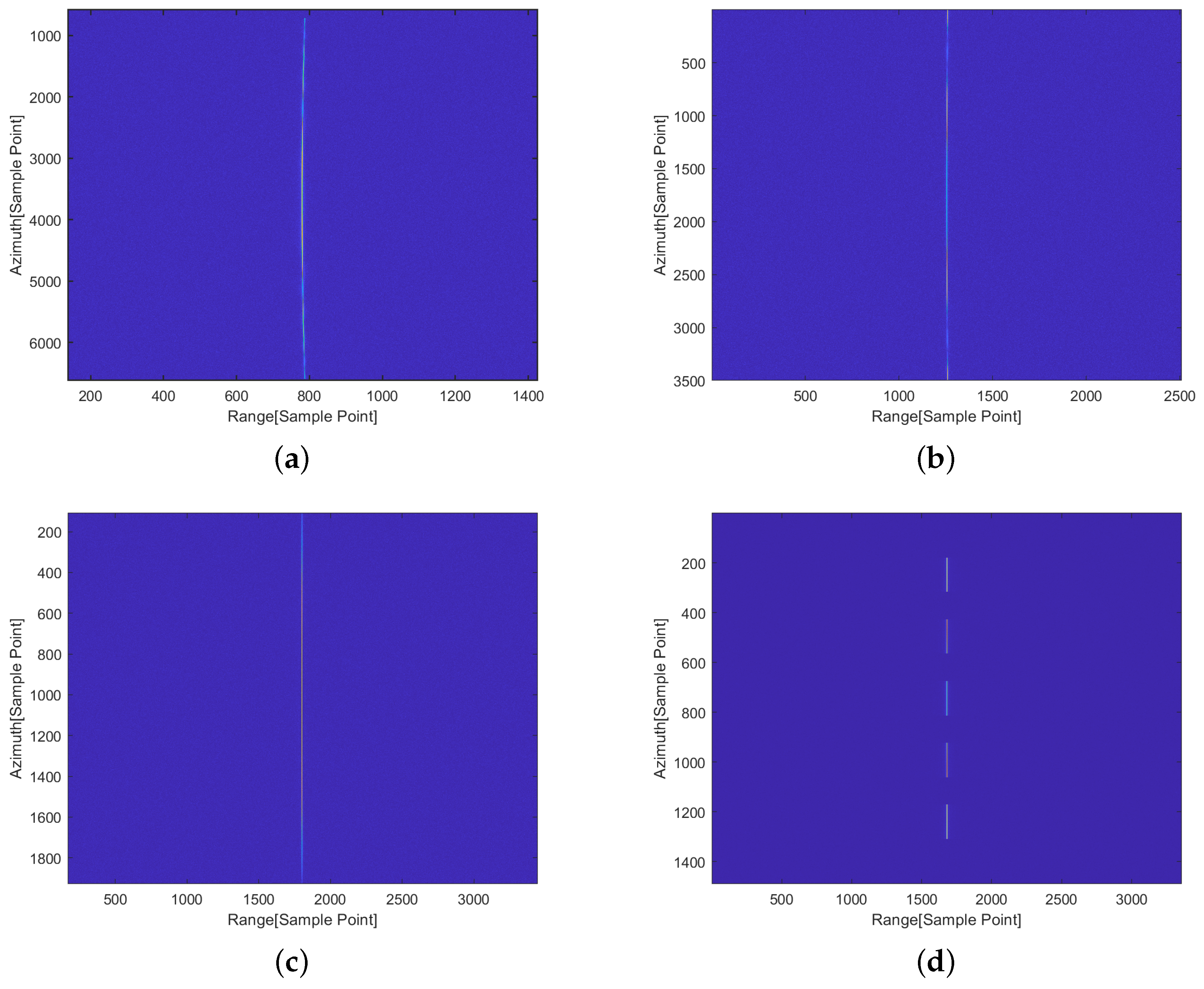
3.1. RPC and Azimuth Time–Frequency Analysis

To address the issue of azimuth amplitude variation characteristics becoming blurred due to reduced SNR, RPC technology is employed. This technique compresses the range LFM signal into a narrow-width yet high-amplitude pulse, concentrating its energy and thereby enhancing the SNR. Ideally, the energy of the intercepted signal is focused along a straight line after pulse compression. However, missing pulses in actual detected signals can prevent energy concentration, adversely affecting operating mode recognition. To solve this problem, azimuth signals are extracted and analyzed using time–frequency analysis. For non-cooperative SAR signals, accurate estimation of the chirp rate of the range LFM signal is essential for effective pulse compression. The FRFT algorithm is commonly used for LFM signal parameter estimation [25]. However, high-accuracy parameter estimation with FRFT demands substantial computational resources, limiting its practical application. To overcome this, an improved CFS-FRFT parameter estimation algorithm is proposed.

3.1.1. The RPC Processing

The frequency-domain-matched filter is applied for RPC of the detected signal, with the detected signal in stripmap mode serving as an illustration. Consequently, the expression for the frequency-domain-matched filter is as follows:

$$H\left(f_{\tau }\right)=exp\left\{j\pi {\displaystyle \frac{f_{\tau }^2}{\widehat{k}}}\right\}$$

(5)

where $f_{\tau }$ denotes the range frequency axis, and $\widehat{k}$ denotes the estimate of the chirp rate. Applying the Fourier transform to (1) yields its frequency domain representation:

$$\begin{array}{cc}\hfill S_{\mathrm{SM}}(f_{\tau },t)& ={\int }_{-\infty }^{\infty }{s}_{SM}(\tau ,t)exp\{-j2\pi f_{\tau }\tau \}d\tau \hfill \\ \hfill & =\mathrm{rect}\left({\displaystyle \frac{f_{\tau }}{\left|K_r\right|T_p}}\right){\omega }_{\alpha }(t-t_c)exp[-j\pi {\displaystyle \frac{2R\left(t\right)}{\lambda }}-j2\pi f_{\tau }{\displaystyle \frac{R\left(t\right)}{c}}]exp(-j\pi {\displaystyle \frac{f_{\tau }^2}{K_r}})\hfill \end{array}$$

(6)

Multiplying (5) and (6) gives:

$$S_{\mathrm{SM}}(f_{\tau },t)H\left(f_{\tau }\right)=\mathrm{rect}\left({\displaystyle \frac{f_{\tau }}{|K_r|T_p}}\right){\omega }_a(t-t_c)exp[-j\pi {\displaystyle \frac{2R\left(t\right)}{\lambda }}-j2\pi f_{\tau }{\displaystyle \frac{R\left(t\right)}{c}}]exp\left[j\pi f_{\tau }^2{\displaystyle \frac{(K_r-\widehat{k})}{K_r\widehat{k}}}\right]$$

(7)

When the relative error of the chirp rate remains below 0.01, $exp\left[j\pi f_{\tau }^2{\displaystyle \frac{(K_r-\widehat{k})}{K_r\widehat{k}}}\right]\approx 1$. In this case, the stripmap intercepted signal after RPC is:

$$\begin{array}{cc}\hfill s_{\text{SM-RPC}}(\tau ,t)& =F_{\tau }^{-1}\left\{S_{SM}(f_{\tau },t)H\left(f_{\tau }\right)\right\}\hfill \\ \hfill & ={\omega }_a(t-t_c)\mathrm{Sinc}\left({\displaystyle \frac{\tau -\frac{R\left(t\right)}{c}}{T_p}}\right)exp(-j\pi {\displaystyle \frac{2R\left(t\right)}{\lambda }})\hfill \end{array}$$

(8)

where $F_{\tau }^{-1}\{·\}$ denotes the range inverse Fourier transform, and $\mathrm{Sinc}(·)$ denotes the sinc function. Similarly, the signal expression following pulse compression in other operating modes can be derived as:

$$s_{\text{SL-RPC}}(\tau ,t)=\mathrm{rect}\left({\displaystyle \frac{t-t_c}{T_{spot}}}\right){\omega }_{\alpha }(t-t_c)\mathrm{Sinc}\left({\displaystyle \frac{\tau -\frac{R\left(t\right)}{c}}{T_p}}\right)exp(-j\pi {\displaystyle \frac{2R\left(t\right)}{\lambda }})$$

(9)

$$s_{\text{SSL-RPC}}(\tau ,t)=\mathrm{rect}\left({\displaystyle \frac{{\nu }_{f}t-x_0}{X}}\right){\omega }_a(t-t_c)\mathrm{Sinc}\left({\displaystyle \frac{\tau -\frac{R\left(t\right)}{c}}{T_p}}\right)exp(-j\pi {\displaystyle \frac{2R\left(t\right)}{\lambda }})$$

(10)

$$s_{\text{Scan-RPC}}(\tau ,t)=\sum _{n=1}^{N_a}\mathrm{rect}\left({\displaystyle \frac{t-n{T}_r}{T_b}}\right){\omega }_a(t-t_c)\mathrm{Sinc}\left({\displaystyle \frac{\tau -\frac{R\left(t\right)}{c}}{T_p}}\right)exp(-j\pi {\displaystyle \frac{2R\left(t\right)}{\lambda }})$$

(11)

The signals described in Equations (8)–(11) are simulated, and the RPC amplitude maps for the detected signals under various operating modes are shown in Figure 8. The results indicate that, after RPC, the signal energy is concentrated along a straight line, significantly enhancing noise immunity. Even at an SNR of 0 dB, the characteristics of the intercepted signals remain distinct across different operating modes. Figure 8a illustrates the pulse compression amplitude map in stripmap mode, where the highest concentration is observed at the center, gradually decreasing towards the azimuth ends with notable variation. In contrast, Figure 8b shows a more uniform azimuth distribution of pulse compression amplitude in spotlight mode. Figure 8c reveals that the pulse compression amplitude map in sliding spotlight mode exhibits characteristics like strip mode but with a smoother transition. Figure 8d demonstrates that the pulse compression amplitude map in scan mode is discontinuous, resembling a windowed truncation of the stripmap mode amplitude map. These results demonstrate that the RPC amplitude map of the intercepted signal encapsulates the operating mode characteristics of the SAR system, offering superior noise resistance and energy concentration. This makes it a more robust basis for discriminating between SAR operating modes.

3.1.2. Azimuth Time–Frequency Analysis

Although pulse compression can enhance the SNR to some extent, the actual intercepted signals may exhibit missing pulses, leading to discontinuous or misaligned RPC results, which complicates operating mode identification. To address this issue, a method is proposed that extracts the peak values of the RPC amplitude along the azimuth direction and performs time–frequency analysis. Equations (8)–(11) indicate that the range signal after pulse compression transforms into a Sinc function, with peak positions determined by the instantaneous slant range between the reconnaissance receiver and the SAR system. Therefore, extracting the peak of the RPC amplitude along each azimuth line yields the azimuth intercepted signals. The azimuth signals for the four modes after peak extraction are represented by Equations (12)–(15).

$$s_{\text{SM-Azimuth}}\left(t\right)={\omega }_a(t-t_c)exp(-j\pi {\displaystyle \frac{2R\left(t\right)}{\lambda }})$$

(12)

$$s_{\text{SL-Azimuth}}\left(t\right)=\mathrm{rect}\left({\displaystyle \frac{t-t_c}{T_{spot}}}\right){\omega }_a(t-t_c)exp(-j\pi {\displaystyle \frac{2R\left(t\right)}{\lambda }})$$

(13)

$$s_{\text{SSL-Azimuth}}\left(t\right)=\mathrm{rect}\left({\displaystyle \frac{{\nu }_{f}t-x_0}{X}}\right){\omega }_a(t-t_c)exp(-j\pi {\displaystyle \frac{2R\left(t\right)}{\lambda }})$$

(14)

$$s_{\text{Scan-Azimuth}}\left(t\right)=\sum _{n=1}^{N_a}\mathrm{rect}\left({\displaystyle \frac{t-n{T}_r}{T_b}}\right){\omega }_a(t-t_c)exp(-j\pi {\displaystyle \frac{2R\left(t\right)}{\lambda }})$$

(15)

The azimuth signals mentioned above has been simulated, and the corresponding results are depicted in Figure 9. Analysis of Figure 9 reveals that the azimuth signal fundamentally represents an LFM signal. However, distinct presentation formats arise due to the unique characteristics of different modes.

To better visualize the azimuth signal waveforms across different modes and enhance the algorithm’s noise immunity, the STFT is applied to process the azimuthal signals. STFT offers localized time–frequency analysis and high computational efficiency, making it suitable for practical engineering applications and improving the overall speed of the operating mode recognition algorithm. Figure 10 presents the STFT simulation results for azimuth signals in four operating modes. The results demonstrate that the time–frequency diagrams of these signals exhibit distinct features, are less noise-sensitive, and display clearer energy aggregation patterns, facilitating easier recognition.

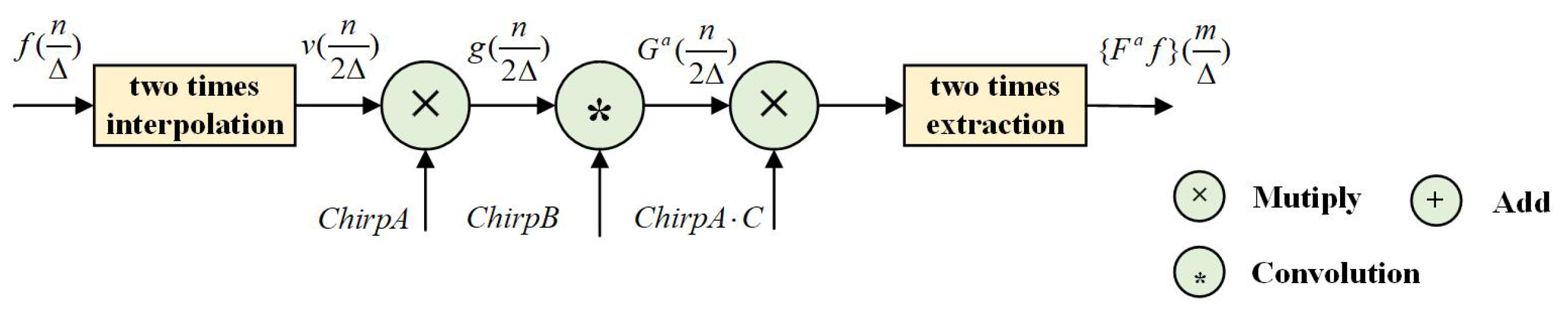
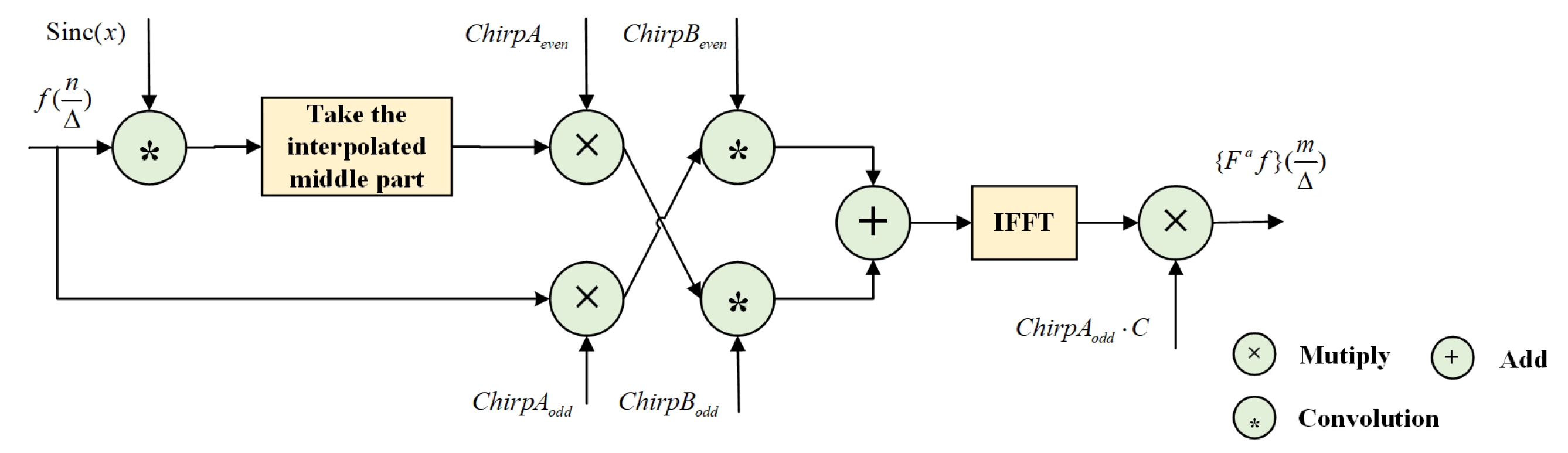
3.2. The Improved CFS-FRFT Algorithm

The FRFT is widely used for detecting and estimating parameters of LFM signals [26,27]. In the FRFT domain, signal energy becomes highly concentrated, exhibiting an impulsive pattern, when the rotation angle corresponds to the optimal order of the LFM signal [28,29]. By identifying the order and frequency associated with this impulsive pattern, key parameters such as the chirp rate and center frequency of the LFM signal can be precisely estimated.

Assume that the LFM signal containing Gaussian white noise is modeled as [30]:

$$s\left(t\right)=A_{0}exp\left[j2\pi (f_{0}t+{\displaystyle \frac{1}{2}}k{t}^2)\right]+n\left(t\right)-{\displaystyle \frac{T}{2}}\le t\le {\displaystyle \frac{T}{2}}$$

(16)

where is $A_0$ the amplitude, T is the pulse width, $f_0$ is the center frequency, k is the chirp rate, and $n\left(t\right)$ represents Gaussian white noise. The estimated values ${\widehat{f}}_0$ and $\widehat{k}$ of the center frequency and chirp rate for the noisy LFM signal, along with the relationship between the fractional order $p_0$ and the fractional domain coordinate $u_0$ corresponding to the energy concentration peak in the FRFT domain, are given by [31]:

$$\left\{\begin{array}{c}{\widehat{f}}_0={\widehat{u}}_{0}csc({\widehat{p}}_0\pi /2)\hfill \\ \widehat{k}=-cot({\widehat{p}}_0\pi /2)f_s/T\hfill \end{array}\right.$$

(17)

where $f_s$ is the sample frequency. The traditional FRFT algorithm, as shown in Figure 11 and proposed by Ozaktas [32], relies on the step size of the search process for estimation accuracy; while a smaller step size improves precision, it significantly increases computational cost. To address this, Tao, R. et al. developed the FRFT2 algorithm [33], as shown in Figure 12, which divides the interpolation process into the original sequence and additional interpolated sequences, enabling separate processing and reducing computational complexity. However, despite its improved computational efficiency, the FRFT2 algorithm is less stable and more vulnerable to noise compared to the traditional FRFT.

In practical applications, SAR signals often involve substantial data volumes. To balance noise resilience, estimation accuracy, and computational complexity, researchers have proposed a CFS-FRFT algorithm [34] to reduce computational demands. This manuscript introduces an enhanced CFS-FRFT algorithm that incorporates the FRFT2 algorithm, with the following steps:

(1) Perform FRFT on the signal across different orders using a coarse search step $\Delta p_1$ within the interval $[-1,1]$, and determine the coarse estimate of the optimal order ${\widehat{p}}_1$ by locating the peak coordinates in the FRFT domain.

(2) Conduct FRFT2 on the signal across different orders using a fine search step $\Delta p_2=\Delta p_1/100$ within the refined interval $[{\widehat{p}}_1-\Delta p_2,{\widehat{p}}_1+\Delta p_2]$, and identify the peak coordinates $(p_0,u_0)$ in the FRFT2 domain.

(3) Substitute $(p_0,u_0)$ into Equation (15) to derive the estimated signal parameters.

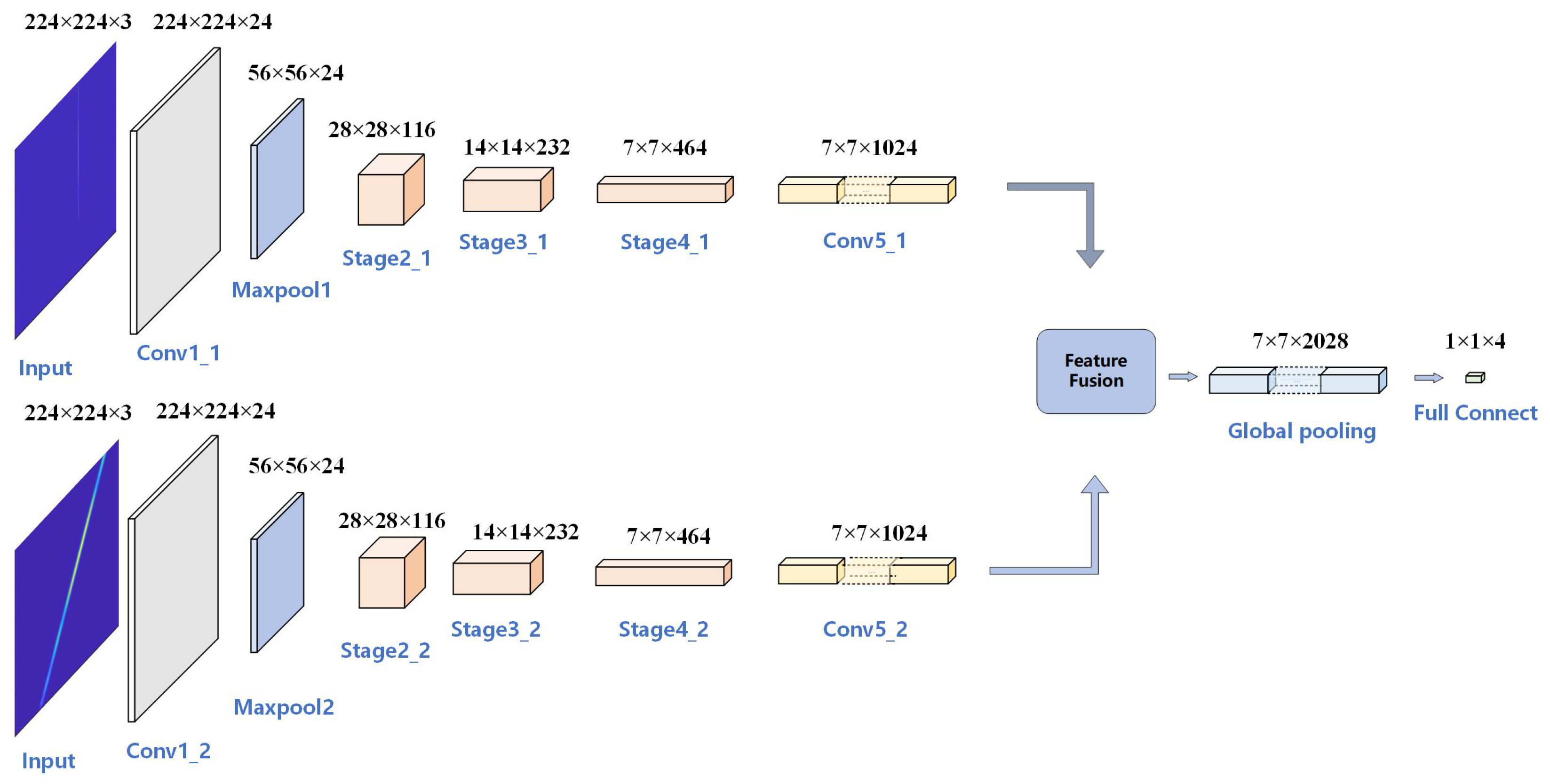
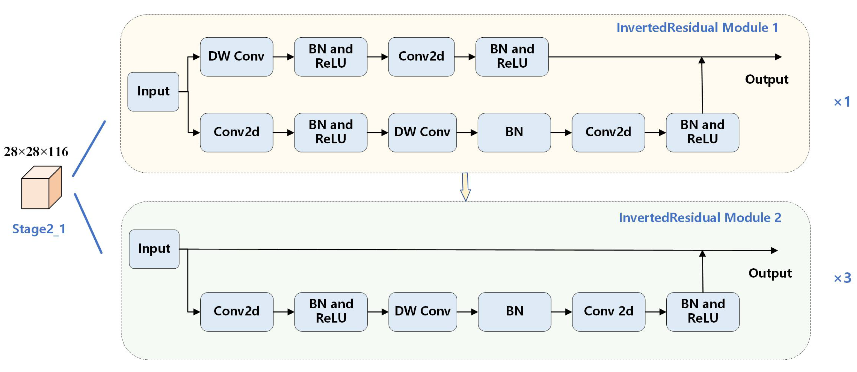
3.3. The Proposed DIFF-ShuffleNet

Traditional CNNs are often constrained by their substantial memory and computational demands, making them unsuitable for mobile and embedded devices and restricting their practical engineering applications. In 2018, a network named ShuffleNet v2 was introduced, which achieves high efficiency and accuracy through four design principles: balanced channel widths, moderate group convolutions, reduced network fragmentation, and emphasis on element-wise operations [35]. Compared to traditional CNNs and other lightweight networks, ShuffleNet v2 demonstrates superior performance across various platforms and tasks. However, the original ShuffleNet v2 is limited to extracting and classifying features from single-input images, making it unsuitable for complex multi-source information fusion tasks. To address this limitation and simultaneously capture feature information from both RPC maps and azimuth time–frequency maps, a dual-input ShuffleNet with adjustable feature weights, termed DIFF-ShuffleNet, is proposed. As illustrated in Figure 13, the network architecture is designed to account for the distinct characteristics of the two input features. Separate feature extraction branches are constructed for the RPC amplitude map and azimuth time–frequency map to maximize the capture of their respective features. Additionally, an effective fusion mechanism is introduced to integrate features from both branches at appropriate network layers, with adjustable weights to optimize the fusion process. This DIFF-ShuffleNet not only handles multi-source information effectively but also enhances the model’s ability to interpret and represent complex signals, significantly improving recognition accuracy.

The proposed network architecture consists of two symmetric branches, each processing either the RPC map or the azimuth time–frequency map. Taking one branch as an example, the input image first passes through a convolutional layer, followed by max pooling, and then proceeds through three stages, each containing multiple inverted residual modules. As illustrated in Figure 14, Stage2_1 comprises four inverted residual modules. Each module has two branches, with the first module differing from the others in its first branch. The first branch of the initial module performs down sampling and channel adjustment via depthwise (DW) convolution, batch normalization (BN), and 2D convolution (conv2d), providing a suitable foundation for subsequent feature extraction and fusion. In contrast, the first branch of the remaining modules retains information without additional operations. Stage3_1 and Stage4_1 follow a similar structure, with Stage3_1 containing eight inverted residual modules and Stage4_1 containing four. In both stages, only the first module aligns with the structure of the first inverted residual module, while the rest match the second. Through these three stages, the network progressively adjusts the feature map dimensions and channel numbers, transforming the input image from pixel-level representation to a more advanced and discriminative feature representation. This process provides a robust feature base for subsequent classification. Conv5_1 primarily adjusts the channel count to prepare for feature fusion, which combines the feature information from both branches using adjustable weights. This fusion mechanism allows the network to leverage information from both branches, enhancing performance and expressive capability. Finally, global pooling reduces the spatial dimensions, and a fully connected layer completes the classification task.

The feature fusion is performed by fusing the feature information of branch one and branch two with certain weights, and the expression of this process is:

$$y_{DIFF}=a\times F_1+b\times F_2$$

(18)

where $F_1$ and $F_2$ represent the input feature information for branch1 and branch2, respectively. Parameters a and b correspond to the weight factors attributed to branch1 and branch2, allowing for adjustable tuning to better align with the processing needs of real SAR data. The output information post feature fusion is denoted by $y_{DIFF}$.

The cross-entropy (CE) loss function is employed for training, a widely used metric in deep learning to quantify the difference between two probability distributions. In the context of multi-classification tasks, assuming the actual label of a sample forms a probability distribution $\overrightarrow{y}$ = ($y_1$, $y_2$, ⋯, $y_n$) across n categories, where $y_i$ signifies the likelihood of the sample belonging to the $i_{th}$ category. The model’s predicted probability distribution is denoted as $\overrightarrow{p}$ = ($p_1$, $p_2$, ⋯, $p_n$), with $p_i$ indicating the probability that the model assigns the sample to the $i_{th}$ category. Consequently, the CE loss function $L_{CE}$ is computed as [36]:

$$L_{CE}=-\sum _{i=1}^n{y}_{i}log\left(p_i\right)$$

(19)

In addition to loss, accuracy is also used to describe the training process of the neural network, and the accuracy indicates the prediction accuracy of the pre-trained model on the validation set, and the expression for the accuracy is:

$$Acc={\displaystyle \frac{T{P}_{SM}+T{P}_{SL}+T{P}_{SSL}+T{P}_{Scan}}{N_{walid}}}$$

(20)

where $T{P}_{SM}$, $T{P}_{SL}$, $T{P}_{SSL}$, and $T{P}_{Scan}$ represent the count of accurately predicted samples in stripmap, spotlight, sliding spotlight, and scan mode, correspondingly. $N_{valid}$ signifies the total number of samples contained within the validation set.

4. Results

4.1. Performance Comparison of Parameter Estimation Algorithms

To validate the ability of the improved CFS-FRFT algorithm to ensure estimation accuracy and noise immunity, 100-time Monte Carlo experiments on parameter estimation of LFM signals are carried out using four methods: the conventional FRFT (with a search step of 0.001) [32], CFS-FRFT [34], CFS-FRFT2, and the proposed algorithm. To better simulate actual SAR signal data, the main parameters of the LFM signals used in the simulation are listed in

Table 2. The main parameters of the LFM signal used in simulations.

Parameter Name	Value
Normalized Amplitude	1
Pulse Width	10 $\mathsf{\mu }$s
Bandwidth	800 MHz
Center Frequency	600 MHz
Sampling Frequency	2.4 GHz

. The normalized root mean square error (NRMSE) is adopted as the evaluation metric. The SNR ranged from −15 dB to 0 dB with a step of 1 dB. The curve of the NRMSE of the chirp rate varying with SNR is shown in Figure 15.

As can be seen from Figure 15, the noise immunity of the proposed algorithm is comparable to that of the CFS-FRFT algorithm. Both can achieve a normalized NRMSE of less than 0.01 for the chirp rate estimation of LFM signals at an SNR of −10 dB. The noise immunity of the proposed algorithm is 1 dB lower than that of the FRFT algorithm with a search step of 0.001. To evaluate computational efficiency, parameter estimation is performed 10 times for each of the four algorithms. The runtime of each trial is measured, and the average value is subsequently calculated. The software used is MATLAB R2021a, and the host computer processor model is 12th Gen Intel(R) Core(TM) i5-1240P 1.70 GHz. The minimum SNR for effective estimation and average running time of the four algorithms for parameter estimation are compared in

Table 3. Minimum SNR for efficient estimation and average parameter estimation runtime under different algorithms.

Algorithm	The Minimum SNR for Effective Estimation	Average Running Time
FRFT (0.001)	−11 dB	84.108 s
CFS-FRFT	−10 dB	8.088 s
CFS-FRFT2	−5 dB	4.424 s
Ours	−10 dB	4.645 s

. The results indicate that for the estimation of SAR signals with preset parameters, the average running time of the proposed algorithm is nearly four seconds less than that of the CFS-FRFT algorithm and over eighty seconds less than that of the FRFT algorithm with a search step of 0.001. Its average running time is equivalent to that of the CFS-FRFT2 algorithm, but the noise immunity of the proposed algorithm is 5 dB higher than that of the CFS-FRFT2 algorithm. Overall, the proposed algorithm improves real-time performance while maintaining effective estimation accuracy and noise immunity, which is conducive to practical engineering applications.

Given that algorithm running time may vary with device encoding efficiency, computational complexity analysis for four algorithms is conducted to ensure robust comparison. For a signal with N sampling points, the computational complexities of FRFT and FRFT2 operations are $O(36N{log}_{2}N+84N)$ and $O(24N{log}_{2}N+35N)$ [33]. For the FRFT algorithm with a search step size of 0.001, it requires a total of 2000 FRFT operations within the order range of [−1, 1]. Since $\Delta p_1$ is set to 0.1 and $\Delta p_2$ is set to 0.001 in the simulation, the CFS-FRFT algorithm performs 20 FRFT operations within the order range of [−1, 1], followed by 200 FRFT operations in the interval $[-0.1+{\widehat{p}}_1,{\widehat{p}}_1+0.1]$, and a total of 220 FRFT operations. Similarly, the CFS-FRFT2 algorithm initially conducts 20 FRFT2 operations in the range of [−1, 1], followed by 200 FRFT2 operations in the interval $[-0.1+{\widehat{p}}_1,{\widehat{p}}_1+0.1]$, culminating in a total of 220 FRFT2 operations. The proposed algorithm performs 20 FRFT operations in the range of [−1, 1] and then executes 200 FRFT2 operations within the interval $[-0.1+{\widehat{p}}_1,{\widehat{p}}_1+0.1]$. The overall computational complexity of the four algorithms is summarized in

Table 4. Computational complexity of different algorithms.

Algorithm	Computational Complexity
FRFT (0.001)	O(72,000Nlog2N + 168,000N)
CFS-FRFT	O(7920Nlog2N + 18,480N)
CFS-FRFT2	O(5280Nlog2N + 7700N)
Ours	O(5520Nlog2N + 8680N)

. It is illustrated by Table 4 that the computational complexity of the proposed algorithm lies between that of the CFS-FRFT algorithm and the CFS-FRFT2 algorithm. However, the proposed algorithm exhibits significantly greater noise resistance compared to the CFS-FRFT2 algorithm. Consequently, the overall performance of the proposed algorithm is superior.

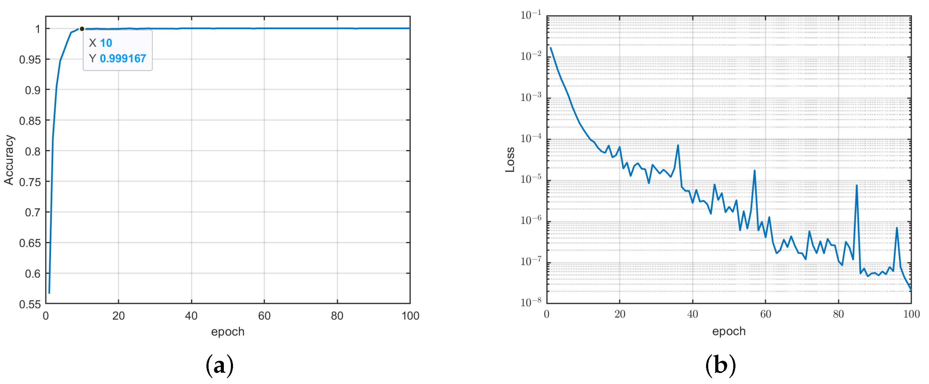
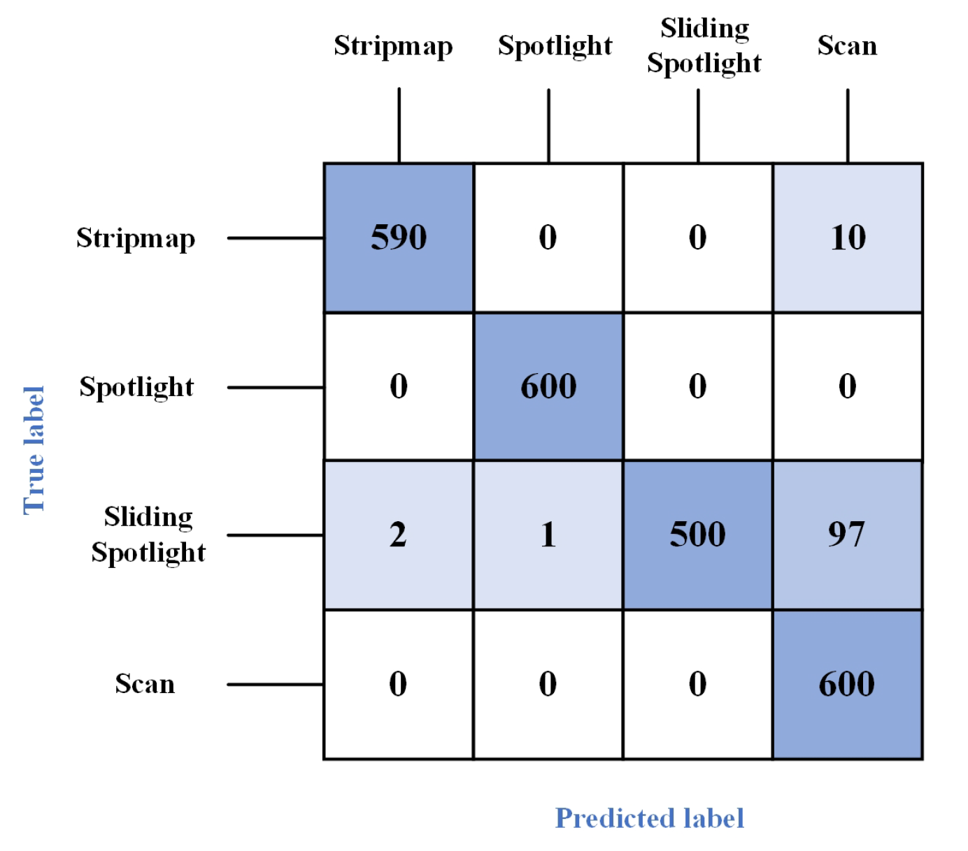
4.2. Analysis of DIFF-ShuffleNet Recognition Performance

The learning rate for the improved dual-input feature fusion neural network is set to 0.00001, with a batch size of 64. The weights for $F_1$ and $F_2$ are set to 0.2 and 0.8, respectively. The software used are MATLAB R2021a and PyCharm Community Edition 2023.2.5. To ensure the proposed SAR operating mode recognition algorithm adapts to low SNR conditions, datasets are generated for four operating modes with SNR ranging from −16 dB to 12 dB in 2 dB increments. The parameters of the detected signals for each mode align with those in Table 1. Additionally, the position of the reconnaissance receiver is randomly varied within ±500 m relative to the (0, 0) coordinate point in the azimuth direction. The dataset is divided into training, testing, and validation sets in a 7:2:1 ratio. The training and validation sets are input into the proposed DIFF-ShuffleNet, which is trained for 100 epochs. The loss function and accuracy change curves during this process are illustrated in Figure 16.

Figure 16 demonstrates that the model achieves a validation set accuracy exceeding 99.9% by the tenth epoch. Consequently, the SAR operating mode recognition model saved at the tenth epoch is utilized to evaluate the test set, with the resulting confusion matrix presented in Figure 17. The results indicate that the model performs well in recognizing stripmap, spotlight, and scan modes, though some confusion arises between sliding spotlight and scan modes. A comparison of the proposed algorithm’s recognition rates with existing algorithms across different SNRs is shown in

Table 5. Recognition rates corresponding to different algorithms at different SNRs.

SNR	−8 dB	−4 dB	0 dB	4 dB	8 dB	12 dB
Accuracy [15]	77.16%	82.10%	84.57%	80.73%	87.35%	88.58%
Accuracy [17]	89.81%	91.67%	91.67%	90.74%	90.43%	91.35%
RPC maps with ShuffleNet	88.13%	90.00%	97.50%	99.38%	99.38%	99.38%
Ours	95.00%	96.25%	96.25%	95.63%	97.50%	99.38%

. The results reveal that the proposed algorithm maintains a comprehensive recognition rate above 95% for SAR operating modes when SNR is not less than −8 dB. When SNR equals −8 dB, the proposed algorithm improves recognition accuracy by nearly 5.2% compared to the method in [17], while also enabling the recognition of sliding spotlight mode. Comparative simulations are also conducted between the proposed algorithm and the baseline method using only RPC maps with ShuffleNet. The results demonstrate that the recognition rate of the proposed algorithm is significantly improved under low SNR conditions, validating the effectiveness of the DIFF-ShuffleNet.

When processing the intercepted SAR signal, the utilization of an increased number of pulses theoretically enhances the comprehensiveness of information within the SAR operating mode, thereby potentially elevating the recognition rate. However, this augmentation in pulses corresponds to a rise in signal processing duration. Therefore, achieving a higher recognition rate with a reduced number of pulses holds significant practical utility. Hence, an investigation into the correlation between the number of detected signal pulses and the recognition rate of the proposed SAR operating mode algorithm is conducted, aiming to offer insights for practical engineering implementations.

The experiment involves configuring the number of detected signal pulses as 200, 400, 600, 800, and 1000, respectively. Subsequently, the trained recognition model is applied to test the dataset with an SNR of 12 dB. The recognition rates of the algorithm employing varying numbers of pulses are tabulated in

Table 6. Recognition rate of different algorithms with different number of pulses (SNR = 12 dB).

Pulse Number	Accuracy
	Algorithm [17]	Ours
200	78.09%	82.50%
400	87.65%	95.63%
600	90.12%	98.13%
800	88.89%	94.38%
1000	91.36%	95.00%

. Analysis of the results in Table 6 reveals that at an SNR of 12 dB, the recognition rate of the proposed algorithm for the test set utilizing 200 pulses exhibits an improvement of at least 4% compared to the algorithm referenced in the literature [17]. Moreover, for all other cases, the recognition rate surpasses 94%. This underscores the adaptability of the proposed algorithm to scenarios involving signal detection with a reduced number of pulses, demonstrating its efficacy for practical applications.

4.3. Actual SAR Data Processing

All the above tests are conducted on simulated data. To ensure the generated SAR operating mode recognition model adapts to actual SAR data, eight sets of actual SAR data are obtained from a cooperative SAR reconnaissance system. The eight sets of data consist of four sets of stripmap SAR data and four sets of spotlight SAR data. The RPC maps and azimuth time–frequency maps of two sets of strip SAR data and two sets of spotlight SAR data are taken for data augmentation. Through data augmentation, the two sets of stripmap data generate 280 RPC maps and 280 azimuth time–frequency maps. Given the high SNR of the actual SAR data, the 280 RPC maps and time–frequency maps with high SNR in the original training set are replaced by the generated maps. The same procedure is applied to the two sets spotlight SAR data. Furthermore, the remaining four sets actual data are reserved for testing, providing their RPC maps and azimuth time–frequency maps as the test set.

The RPC maps and azimuth time–frequency maps for the remaining four sets of SAR-measured data are shown in Figure 18. They are used as inputs for the updated recognition model, with the original information and recognition results for the four datasets detailed in

Table 7. Original information and recognition results of four sets of actual SAR data.

Data Name	SAR Platform	Wave Band	Actual Operating Mode	Recognition Results	Correctness
Data1.dat	Airborne	Ku	Stripmap	Stripmap	Correct
Data2.dat	Spaceborne	C	Spotlight	Spotlight	Correct
Data3.dat	Spaceborne	C	Spotlight	Spotlight	Correct
Data4.dat	Airborne	Ku	Stripmap	Stripmap	Correct

. The results demonstrate that the proposed algorithm accurately identifies the operating modes for all four SAR datasets, confirming its ability to process actual data.

5. Discussion

As demonstrated by the simulations and analyses in Section 4, the proposed algorithm has a high comprehensive recognition rate for the four SAR operating modes at low SNR; while preliminary validation confirms its ability to process actual SAR data, certain limitations persist in practical applications.

The acquired real SAR data exhibit misaligned pulse compression results, likely attributable to pulse missing induced by the SAR reconnaissance receiver’s sampling mechanism. Notably, this phenomenon does not occur in all SAR data intercepted by the receiver. Since the simulation data do not account for RPC misalignment, the recognition model generated by the simulation data is not effective enough in identifying the actual data. To address this, partial actual SAR data must be incorporated for data augmentation, enabling model retraining to achieve satisfactory recognition accuracy. Future work should integrate pulse compression misalignment into the simulation framework, thereby enhancing the model’s adaptability to actual SAR data processing.

6. Conclusions

This manuscript proposes an algorithm for recognizing SAR operating modes. First, the amplitude differences of detected signals under four modes (stripmap, spotlight, sliding spotlight, and scan) are analyzed. To mitigate the impact of noise on feature differentiation, a novel approach is introduced, utilizing the RPC map and azimuth time–frequency map as classification features. Additionally, a DIFF-ShuffleNet structure is proposed, which integrates the features of the RPC map and azimuth time–frequency map with adjustable weights, leveraging the strengths of both inputs to enhance recognition accuracy. Simulations demonstrate that the algorithm achieves an overall recognition rate exceeding 95.00% for the test set across the four SAR operating modes when the SNR exceeds −8 dB. To address the requirement for chirp rate estimation in the RPC process, an improved CFS-FRFT algorithm is introduced. This algorithm reduces runtime while maintaining noise immunity and estimation accuracy, efficiently estimating the chirp rate of detected signals when SNR exceeds −10 dB. Finally, the recognition model generated by the proposed algorithm is applied to four sets of actual SAR data, successfully identifying the operating modes, and thereby validating its effectiveness in processing actual SAR data.

References

1. Wang, C.; Zhang, Q.; Hu, J.; Li, C.; Shi, S.; Fang, G. An Efficient Algorithm Based on CSA for THz Stepped-Frequency SAR Imaging. IEEE Geosci. Remote Sens. Lett. 2022, 19, 1–5. [Google Scholar] [CrossRef]
2. Wang, C.; Zhang, Q.; Hu, J.; Shi, S.; Li, C.; Cheng, W.; Fang, G. An Efficient Algorithm Based on Frequency Scaling for THz Stepped-Frequency SAR Imaging. IEEE Trans. Geosci. Remote Sens. 2022, 60, 5225815. [Google Scholar] [CrossRef]
3. Cheng, W.; Zhang, Q.; Lu, W.; Wang, H.; Liu, X. An Efficient Digital Channelized Receiver for low SNR and Wideband Chirp Signals Detection. Appl. Sci. 2023, 13, 3080. [Google Scholar] [CrossRef]
4. Dong, J.; Zhang, Q.; Lu, W.; Cheng, W.; Liu, X. Hybrid Domain Efficient Modulation-Based Deceptive Jamming Algorithm for Nonlinear-Trajectory Synthetic Aperture Radar. Remote Sens. 2023, 15, 2446. [Google Scholar] [CrossRef]
5. Liu, Y.; Wang, W.; Pan, X.; Xu, L.; Wang, G. Influence of Estimate Error of Radar Kinematic Parameter on Deceptive Jamming Against SAR. IEEE Sens. J. 2016, 16, 5904–5911. [Google Scholar] [CrossRef]
6. Sun, Q.; Shu, T.; Yu, K.B.; Yu, W. Efficient Deceptive Jamming Method of Static and Moving Targets Against SAR. IEEE Sens. J. 2018, 18, 3610–3618. [Google Scholar] [CrossRef]
7. Liu, H.; Song, H.; Cheng, H. Comparative Study on Stripmap Mode, Spotlight Mode, and Sliding Spotlight Mode. J. Grad. Sch. CAS 2011, 28, 410–417. [Google Scholar]
8. Chen, Y.; Jia, X.; Wu, Y. The Sidelobe Surveillance Study of Spaceborne Synthetic Aperture Radar in Spotlight and Sliding Spotlight Mode. Sci. Technol. Eng. 2012, 12, 1785–1789. [Google Scholar]
9. Chen, Y.; Gao, Y.; He, Y. Optimal Selection of PRF for Spaceborne Synthetic Aperture Radar in Different Working Mode. Mod. Electron. Tech. 2012, 35, 25–28. [Google Scholar]
10. Chen, Y.; Wu, Y.; Jia, X. Surveillance Study of Spaceborne Synthetic Aperture Radar in Different Working Modes. Comput. Eng. Appl. 2013, 49, 223–227+241. [Google Scholar]
11. Tang, X.; Li, C.; Gao, J.; Sun, B. Research on Operation Inversion Method of Spaceborne SAR. Radio Eng. 2012, 42, 33–36. [Google Scholar]
12. Tang, X.; Li, C.; Sun, B. An Operation Inversion Method of Spaceborne SAR Based on Genetic Algorithm. Space Electron. Technol. 2013, 10, 90–94. [Google Scholar]
13. Da, R.; Xin, J.; Yin, C.; Lao, G.; Yang, G. In Synthetic Aperture Radar Operation Mode Recognition Based on Time-Frequency Analysis. In Proceedings of the IET International Radar Conference, Hangzhou, China, 14–16 October 2015; pp. 1–4. [Google Scholar]
14. Xia, Z.; Zhong, H.; Chen, W. Identification of the Spaceborne SAR Operating Modes under Reconnaissance Mode. J. Hangzhou Dianzi Univ. Nat. Sci. 2017, 37, 36–40. [Google Scholar]
15. He, J.; Zhang, Y.; Ying, C. Operating Modes Identification of Spaceborne SAR Based on Deep Learning. J. Zhejiang Univ. Eng. Sci. 2022, 56, 1676–1684. [Google Scholar]
16. He, J.; Zhang, Y.; Ying, C.; Fang, Y. Operating Modes of Spaceborne SAR Recognition Based on CGRU-SVM. Command Control Simul. 2022, 44, 99–105. [Google Scholar]
17. Ma, R.; Jin, G.; Song, C.; Li, Y.; Wang, Y.; Zhu, D. A Novel Method to Identify the Spaceborne SAR Operating Mode based on Sidelobe Reconnaissance and Machine Learning. Remote Sens. 2024, 16, 1234. [Google Scholar] [CrossRef]
18. Chen, J.; Wang, K.; Yang, W.; Liu, W. Accurate Reconstruction and Suppression for Azimuth Ambiguities in Spaceborne Stripmap SAR Images. IEEE Geosci. Remote Sens. Lett. 2017, 14, 102–106. [Google Scholar] [CrossRef]
19. Zhu, D.; Ye, S.; Zhu, Z. Polar Format Agorithm Using Chirp Scaling for Spotlight SAR Image Formation. IEEE Trans. Aerosp. Electron. Syst. 2008, 44, 1433–1448. [Google Scholar] [CrossRef]
20. Belcher, D.; Baker, C. High Resolution Processing of Hybrid Strip-map/Spotlight Mode SAR. In Proceedings of the IEEE Proceedings-Radar, Sonar and Navigation, London, UK, 1 December 1996; pp. 366–374. [Google Scholar]
21. Bamler, R.; Eineder, M. Scansar Processing Using Standard High Precision SAR Algorithms. IEEE Trans. Geosci. Remote Sens. 1996, 34, 212–218. [Google Scholar] [CrossRef]
22. Holzner, J.; Bamler, R. Burst-mode and Scansar Interferometry. IEEE Trans. Geosci. Remote Sens. 2002, 40, 1917–1934. [Google Scholar] [CrossRef]
23. Li, N.; Wang, R.; Deng, Y.; Chen, J.; Zhang, Z.; Liu, Y.; Xu, Z.; Zhao, F. Improved Full-Aperture ScanSAR Imaging Algorithm Based on Aperture Interpolation. IEEE Geosci. Remote Sens. Lett. 2015, 12, 1101–1105. [Google Scholar]
24. Leon, C. Time-Frequency Analysis: Theory and Applications; Pnentice Hall: Englewood Cliffs, NJ, USA, 1995. [Google Scholar]
25. Serbes, A. On the Estimation of LFM Signal Parameters: Analytical Formulation. IEEE Trans. Aerosp. Electron. Syst. 2018, 54, 848–860. [Google Scholar] [CrossRef]
26. Aldimashki, O.; Serbes, A. Performance of Chirp Parameter Estimation in the Fractional Fourier Domains and an Algorithm for Fast Chirp-rate Estimation. IEEE Trans. Aerosp. Electron. Syst. 2020, 56, 3685–3700. [Google Scholar] [CrossRef]
27. Huang, X.; Tang, S.; Zhang, L.; Gu, Y. A Fast Algorithm of LFM Signal Detection and Parameter Estimation Based on Efficient FrFT. J. Electron. Inform. Technol. 2017, 39, 2905–2911. [Google Scholar]
28. Capus, C.; Brown, K. Fractional Fourier Transform of the Gaussian and Fractional Domain Signal Support. In Proceedings of the IEEE Proceedings-Vision Image and Signal Processing, London, UK, 1 April 2003; pp. 99–106. [Google Scholar]
29. Capus, C.; Rzhanov, Y.; Linnett, L. The Analysis of Multiple Linear Chirp Signals. In Proceedings of the IEEE Symposium on Time-Scale and Time-Frequency Analysis and Applications, London, UK, 29 February 2000. [Google Scholar]
30. Qi, L.; Tao, R.; Zhou, S.; Wang, Y. Detection and Parameter Estimation of Multicomponent LFM Signal Based on the Fractional Fourier Transform. Sci. China Ser. F Inform. Sci. 2004, 47, 184–198. [Google Scholar] [CrossRef]
31. Cong, Y.; Li, H.; Wang, J. The parameter estimation of wideband LFM signal based on down-chirp and compressive sensing. In Proceedings of the 2018 IEEE 4th Information Technology and Mechatronics Engineering Conference (ITOEC), Chongqing, China, 14–16 December 2018; pp. 1436–1441. [Google Scholar]
32. Ozaktas, H.M.; Barshan, B.; Mendlovic, D.; Onural, L. Convolution, Filtering, and Multiplexing in Fractional Fourier Domains and Their Relation to Chirp and Wavelet Transforms. J. Opt. Soc. Am. A 1994, 11, 547–559. [Google Scholar] [CrossRef]
33. Tao, R.; Liang, G.; Zhao, X.-H. An Efficient FPGA-Based Implementation of Fractional Fourier Transform Algorithm. J. Signal Process. Syst. 2010, 60, 47–58. [Google Scholar] [CrossRef]
34. Feng, Z. Research on UWB Radar Signal Detection Based on Compressed Sensing. Master’s Thesis, Xidian University, Xi’an China, 2018. [Google Scholar]
35. Ma, N.; Zhang, X.; Zheng, H.-T.; Sun, J. In Shufflenet v2: Practical Guidelines for Efficient CNN Architecture Design. In Proceedings of the European Conference on Computer Vision (ECCV), Munich, Germany, 8–14 September 2018; pp. 116–131. [Google Scholar]
36. Nielsen, M.A. Neural Networks and Deep Learning; Determination Press: San Francisco, CA, USA, 2015; Volume 25. [Google Scholar]
Figure 1. Schematic diagram of stripmap operating mode.
Remotesensing 17 01523 g001
Figure 2. Schematic diagram of spotlight operating mode.
Remotesensing 17 01523 g002
Figure 3. Schematic diagram of sliding spotlight operating mode.
Remotesensing 17 01523 g003
Figure 4. Schematic diagram of scan operating mode.
Remotesensing 17 01523 g004
Figure 5. Amplitude diagrams of intercepted signals in different operating modes (without noise): (a) stripmap; (b) spotlight; (c) sliding spotlight; (d) scan.
Remotesensing 17 01523 g005
Figure 6. Amplitude diagrams of intercepted signals in different operating modes (SNR = 0 dB): (a) stripmap; (b) spotlight; (c) sliding spotlight; (d) scan.
Remotesensing 17 01523 g006aRemotesensing 17 01523 g006b
Figure 7. Schematic diagram of the proposed algorithm.
Remotesensing 17 01523 g007
Figure 8. The RPC amplitude maps of detected signals in different operating modes (SNR = 0 dB): (a) stripmap; (b) spotlight; (c) sliding spotlight; (d) scan.
Remotesensing 17 01523 g008
Figure 9. Waveform of the azimuthal signals in different modes (SNR = 0 dB): (a) stripmap; (b) spotlight; (c) sliding spotlight; (d) scan.
Remotesensing 17 01523 g009
Figure 10. The azimuthal time–frequency diagrams in different operating modes (SNR = 0 dB): (a) stripmap; (b) spotlight; (c) sliding spotlight; (d) scan.
Remotesensing 17 01523 g010
Figure 11. Flowchart of conventional FRFT.
Remotesensing 17 01523 g011
Figure 12. Flowchart of the FRFT2 algorithm.
Remotesensing 17 01523 g012
Figure 13. The structure of the DIFF-ShuffleNet.
Remotesensing 17 01523 g013
Figure 14. Schematic diagram of internal components of stage2_1.
Remotesensing 17 01523 g014
Figure 15. Variation curve of chirp rate NRMSE with SNR under different parameter estimation algorithms.
Remotesensing 17 01523 g015
Figure 16. Curves of accuracy and loss with epoch during training: (a) accuracy; (b) loss.
Remotesensing 17 01523 g016
Figure 17. Classification confusion matrix of the algorithm proposed in this manuscript.
Remotesensing 17 01523 g017
Figure 18. The RPC maps and azimuth time–frequency maps of four sets of actual SAR data. (a) The RPC map of SAR-Data1. (b) The azimuth time–frequency map of SAR-Data1. (c) The RPC map of SAR-Data2. (d) The azimuth time–frequency map of SAR-Data2. (e) The RPC map of SAR-Data3. (f) The azimuth time–frequency map of SAR-Data3. (g) The RPC map of SAR-Data4. (h) The azimuth time–frequency map of SAR-Data4.
Remotesensing 17 01523 g018