Improving the Accuracy of Soil Classification by Using Vis–NIR, MIR, and Their Spectra Fusion

Abstract

Soil spectroscopy offers a rapid, cost-effective alternative to traditional soil analyses for characterization and classification. Previous studies have mainly focused on predicting soil categories using single sensors, particularly visible–near-infrared (vis–NIR) or mid-infrared (MIR) spectroscopy. In this study, we evaluated the performance of vis–NIR, MIR, and their combined spectra for soil classification by partial least-squares discriminant analysis (PLSDA) and random forest (RF). Utilizing 60 typical soil profiles’ data of four soil classes from the global soil spectral library (GSSL), our results demonstrated that in PLSDA models, direct combination (optimal overall accuracy: 70.6%, kappa coefficient: 0.60) and outer product analysis (OPA) fused spectra (optimal overall accuracy: 68.1%, kappa coefficient: 0.57) outperformed vis–NIR (optimal overall accuracy: 62.2%, kappa coefficient: 0.49) but underperformed compared to MIR (optimal overall accuracy: 71.4%, kappa coefficient: 0.62). In RF models, classification accuracy using fused spectra was inferior to single spectral ranges, with MIR achieving the highest classification accuracy (optimal overall accuracy: 89.1%, kappa coefficient: 0.85). Therefore, MIR alone remains the most effective spectral range for accurate soil class discrimination. Our findings highlight the potential of MIR spectroscopy for enhancing global soil classification accuracy and efficiency, with important implications for soil resource management and agricultural planning across diverse environments.

1. Introduction

As a fundamental method in soil science research, accurate soil classification is crucial not only for effective resource management and land use planning but also for crop growth, development, and environmental monitoring [1]. Accurate soil classification can help identify the specific needs of each soil type and facilitate the formulation of tailored management strategies. Traditional soil classification methods rely heavily on field surveys, labor-intensive laboratory analyses, and subjective expert judgment. These approaches are time-consuming, costly, and susceptible to human error. Therefore, there is a critical need for a more precise, efficient, and objective soil analysis method.

In comparison to conventional laboratory methods, soil spectroscopy in the visible-to-near-infrared (vis–NIR) and mid-infrared (MIR) regions offers unparalleled advantages, including rapidity, simplicity, non-destructiveness, cost-effectiveness, and minimal sample requirements [2,3]. Spectroscopic techniques have been widely applied to predicting soil properties [4,5,6], and, to some extent, in soil classification [7,8]. Previous studies on soil classification have primarily used vis–NIR spectroscopy, achieving classification accuracies usually around 60% [8,9,10]. MIR spectroscopy generally provides more accurate estimations of soil properties [11,12]. This is because the vibrational modes in the vis–NIR region mainly correspond to the low-frequency overtone and combination vibrations found in the fundamental vibrations of the MIR region, capturing weaker fundamental and combination bands [13,14]. However, due to technological complexity and cost limitations, the application of MIR spectroscopy in soil classification remains limited. Only a few studies have used MIR spectra for soil type discrimination, achieving higher classification accuracies, often exceeding 70%, with some reaching as high as 95% [15,16]. As is well known, soil resources are essential for national food security, ecological stability, and biodiversity conservation [17,18]. Accurate soil classification is fundamental for effective soil resource planning and management. However, spectral measurements can vary significantly due to environmental factors and sample heterogeneity, regardless of whether the same or different instruments are used. These variations potentially reduce classification accuracy. Therefore, this study will compare the classification accuracies of vis–NIR and MIR under the same conditions.

The inherent limitations of a single sensor and soil complexity restrict accurate soil characterization. Neither vis–NIR nor MIR spectroscopy alone can fully capture the diversity of soil physicochemical properties [19]. Each spectral range is sensitive to different but complementary soil attributes, supporting the need for spectral fusion. Spectral fusion reduces prediction variance and minimizes soil matrix interference, thereby enhancing model stability [20,21]. Combining vis–NIR and MIR data may mitigate the shortcomings of individual spectra and uncover complex soil interactions that individual spectra cannot detect. Spectral data fusion can be categorized into three levels: low-level, middle-level, and high-level [22]. Low-level fusion involves the direct connection and integration of data from different sensors to generate a multi-dimensional dataset. Middle-level fusion focuses on extracting and integrating meaningful features from raw data, providing a richer and more informative foundation for subsequent decision-making and analysis. The Outer Product Analysis (OPA) method has shown particular promise for spectral data fusion in soil science applications [23,24]. This middle-level fusion approach effectively captures complementary information from different spectral regions while minimizing noise and redundancy [25,26]. High-level fusion refers to the integration of final decisions made from multiple independent data sources, often through the use of different algorithms or models.

Many studies have explored the application of multi-sensor data fusion in predicting soil properties. Research indicates that fusing data from different sensors can effectively improve the overall performance of predictive models [27,28]. In particular, single sensors often have limitations in capturing spectral features of certain soil properties, and data fusion can address these shortcomings to achieve more accurate predictions [29,30]. This provides a promising idea to improving the accuracy and efficiency of soil classification. Although applications of spectral data fusion in soil classification remain limited, our group member Xu et al. have demonstrated the potential of spectral fusion methods in previous studies. They classified 146 soil profiles in Zhejiang Province using simple combination and OPA fused spectra. The results showed that the simple combination presented an accuracy of 61.1%, which was the lowest, while the OPA fused spectra achieved the highest accuracy of 68.4% [31]. This validates the effectiveness of the OPA method for soil classification at a regional scale.

Recent advances in spectral fusion techniques have demonstrated potential for improving soil property predictions. However, their application to soil classification at a global scale remains largely unexplored, particularly when comparing the relative performance of single-sensor versus fused-sensor approaches across diverse soil classes. In addition, previous studies primarily focus on using spectral fusion for predicting soil organic carbon (SOC), fertility parameters, soil aggregate, and other soil properties [3,11,32,33], while its application in soil classification remains limited. There is currently no panacea for data fusion methods that work in all conditions. Meanwhile, the benefits of sensor fusion in proximal soil sensing are still controversial. Their effectiveness may depend on specific application contexts and data attributes. Researchers must continually explore and experiment to find the most suitable fusion strategies for varying data characteristics and requirements. Consequently, the purposes of this study are as follows: (1) to compare the model accuracy of single-sensor (vis–NIR or MIR) spectroscopy in soil classification; (2) to evaluate the performance of single-sensor versus sensor fusion in soil classification.

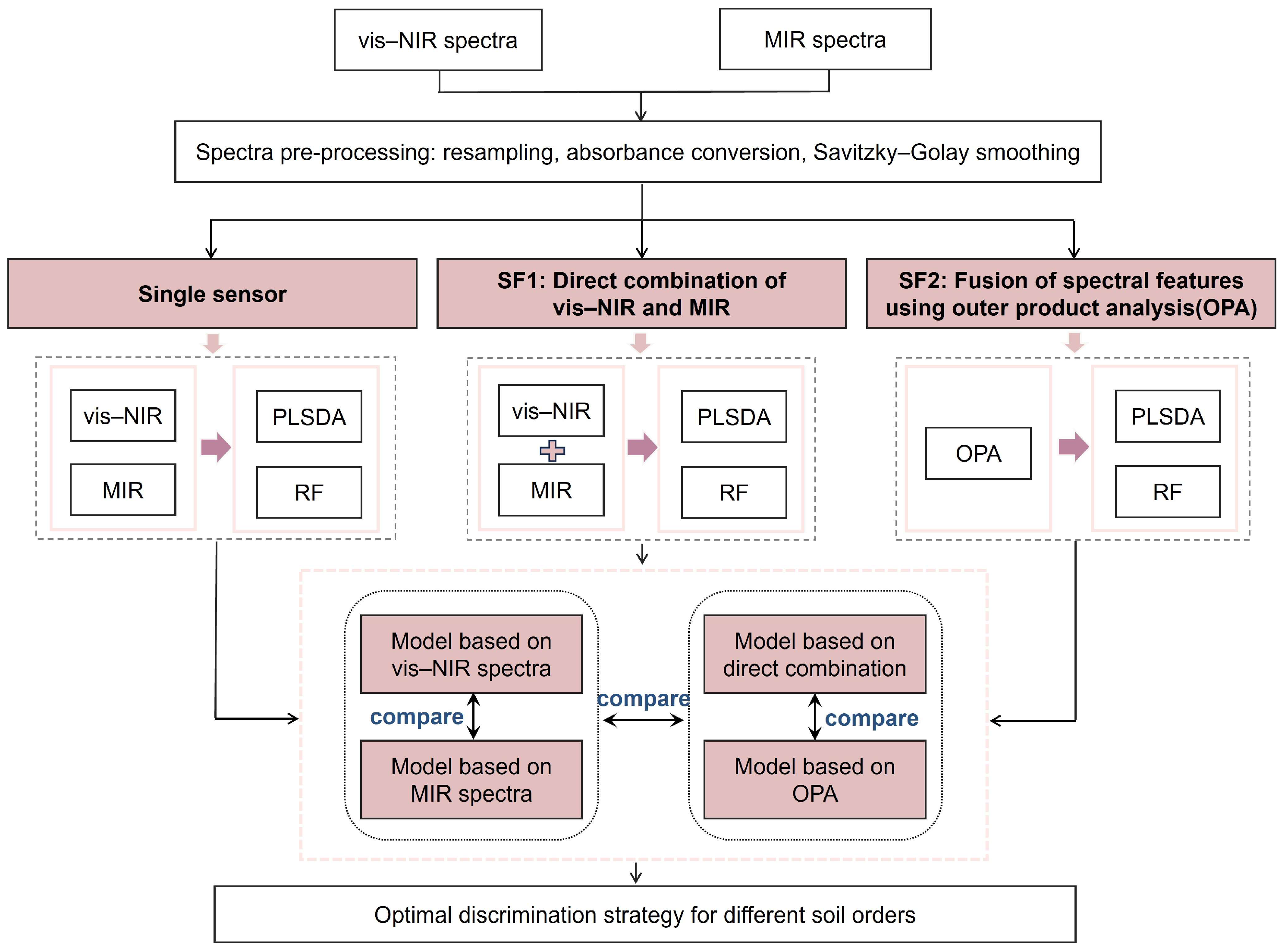
2. Materials and Methods

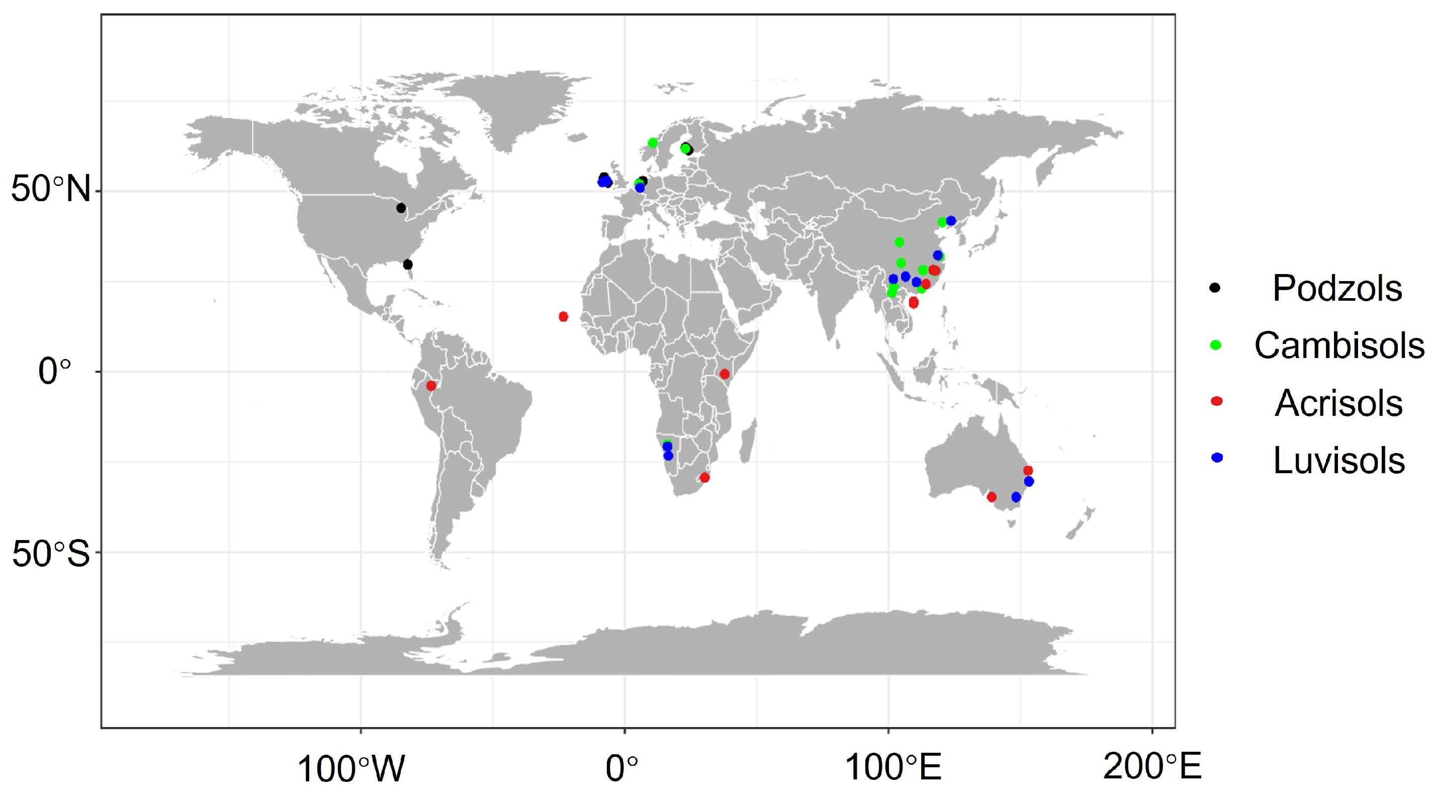
2.1. Data Source

The spectra data we used were sourced from the Global Soil Spectral Library (GSSL), which encompasses a vis–NIR and a MIR soil spectra dataset described by Viscarra Rossel et al. [34] and Terhoeven-Urselmans et al. [35], respectively. The dataset across Asia, Africa, Europe, North America, and South America was compiled by the World Agroforestry (ICRAF) and the International Soil Reference Information Center (ISRIC) through spectral scanning at the Soil and Plant Spectral Diagnostics Laboratory. Before spectral measurements, all soil samples were air-dried, ground, and sieved to a particle size of 2 mm. The vis–NIR spectra were collected using FieldSpec^®FR spectroradiometer (Analytical Spectral Devices, Boulder, CO, USA). The spectra range covered wavelengths from 350 to 2500 nm at 1 nm intervals. The MIR spectra, covering the range from 7496 to 600 cm⁻¹, were obtained using a Tensor 27 FTIR spectrometer (Bruker Optics, Karlsruhe, Germany), with a sampling interval of 2 cm⁻¹. Overall, a total of 4438 soil samples from 785 soil profiles were retained, and Figure 1 presents the spatial distribution of 60 profiles from four soil classes in GSSL.

The dataset also provides soil classifications systems based on the World Reference Base for Soil Resources (WRB) and the Food and Agriculture Organization (FAO). However, not all samples are classified according to the WRB system, and a number of them lack WRB classification information. From this, 151 soil profiles were selected for the study (

Table 1. Summary statistics of soil profiles and samples across 26 WRB reference groups.

Soil Class	Numbers of Profiles/Samples	Soil Class	Numbers of Profiles/Samples
Cambisols	17/84	Fluvisols	4/27
Luvisols	16/85	Alisols	3/21
Podzols	14/99	Albeluvisols	3/19
Acrisols	13/89	Planosols	3/24
Arenosols	9/51	Plinthosols	3/20
Phaeozems	9/42	Umbrisols	3/16
Anthrosols	7/28	Chernozems	2/12
Ferralsols	7/40	Gypsisols	2/14
Vertisols	7/47	Gleysols	2/9
Andosols	6/28	Regosols	2/11
Solonetzs	6/47	Cryosols	1/6
Nitisols	5/36	Durisols	1/6
Lixisols	5/22	Kastanozems	1/8

), representing 26 primary soil units. Due to differences in pedogenesis, the profile structure, number of sampled horizons, and sampling depth vary among soil classes, resulting in uneven sample numbers. Among them, Podzols include 14 profiles, but they have the highest number of samples, reaching 99, because of the well-developed profiles with more horizons. Nevertheless, Kastanozems, Cryosols, and Durisols have very few samples, with only one profile each, due to their limited distribution, sampling difficulty, and unique profile development. To ensure the robustness and representativeness of the models, four soil classes with complete WRB classification and relatively sufficient samples were selected for further analysis: Cambisols (17 profiles), Luvisols (16 profiles), Podzols (14 profiles), and Acrisols (13 profiles). These are presented as the top four soil classes in Table 1.

2.2. Spectral Pre-Processing

The vis–NIR and MIR spectra were resampled to 10 nm and 16 cm⁻¹, respectively, retaining the range of 400–2450 nm and 4008–600 cm⁻¹. To further enhance the spectral signals, we adopted two pre-processing methods. Initially, absorbance conversion was performed, transforming spectral reflectance into absorbance using a logarithmic function, and spectral absorption features were emphasized. Subsequently, the Savitzky–Golay filter [36] was applied to remove noise from the spectral data while preserving the shape and width of the signal. After several tests, a 2nd-order polynomial with a window size of 11 was adopted for optimal smoothing. The pre-processing was conducted using the “Prospectr” package in R software (4.3.3).

2.3. Spectra Fusion

Following spectral pre-processing, both low-level and middle-level spectral fusion strategies were implemented separately on the dataset. The overall workflow is presented in Figure 2. The fusion methods are briefly described in the following subsections. This method preserves the original spectral information and allows the model to fully utilize the complementary characteristics of both spectral ranges.

2.3.1. Low-Level Fusion (SF1)

Low-level fusion involves directly concatenating spectra from two or more instruments in the spectral dimension. In this study, 214 resampled MIR absorbance bands were concatenated with 206 vis–NIR absorbance bands, resulting in 420 contiguous fused spectral data.

2.3.2. Middle-Level Fusion (SF2)

Middle-level fusion, or feature fusion, combines features from the original data. OPA is a middle-level data fusion method widely applied in various instrumental analysis domains [23]. The OPA builds an outer product matrix from sample vectors, expanding the matrix to create all possible interaction relationships between the spectral variables of two datasets [24]. It highlights the joint variations and co-evolution patterns in different spectral regions. This is especially important in soil spectroscopy because the relationships between soil properties and spectral responses are nonlinear and interdependent. Many researchers have also confirmed that OPA provides a clearer representation of variable interactions and shows superior performance in soil spectral prediction (see the introduction).

This study utilized OPA for middle-level fusion to identify influential characteristic bands of soil nutrients. The 206 bands from the vis–NIR spectrometer and 214 MIR bands obtained after resampling from the MIR spectrometer were fused to create a new spectral matrix. The fused spectra underwent Principal Component Analysis (PCA) to reduce data redundancy, with the top twenty principal components retained for subsequent analyses.

2.4. Model Construction and Assessment

Soil classification based on spectral information necessitates applying linear methods and machine learning approaches for modeling. In this study, Partial Least-Squares Discriminant Analysis (PLSDA) and Random Forest (RF) classification modeling methods were employed. Sixty soil profiles, comprising 357 soil spectra with corresponding categories, were randomly divided into calibration and validation datasets at a 2:1 ratio. The calibration dataset comprised 238 samples, while the validation dataset comprised 119 samples. The calibration dataset was utilized to establish the relationship between pre-processed spectra and soil types, whereas the validation dataset was used for predicting soil types. Model performance was assessed using the confusion matrix and Kappa coefficient. Overall accuracy and specific analysis of each class’s classification were conducted by calculating sensitivity and accuracy.

2.4.1. Partial Least–Squares Discriminant Analysis (PLSDA)

The PLSDA is a multivariate statistical method employed for discriminant analysis, integrating the strengths of partial least squares regression and discriminant analysis [37]. The method is a supervised classification method based on PLS regression. It aims to find a linear subspace of explanatory variables that maximizes the covariance between the independent variables X (soil spectra) and the dependent variables Y (soil types). Widely used in classification and prediction tasks, PLSDA focuses on identifying latent variables, known as PLS components, which maximize inter-group variability while minimizing intra-group variability. These components help lower data dimensionality and distinguishing between different sample groups [38,39]. The study utilized the PLSDA model through the “ropls” package in the R software (4.3.3).

2.4.2. Random Forest (RF)

The RF algorithm is a popular machine learning technique based on Bagging, introduced by Breiman [40], suitable for both classification and regression tasks. By generating multiple decision tree models and aggregating their results, RF offers several advantages, including independence from multicollinearity, elimination of variable selection, operational efficiency, suitability for larger sample sizes, and robustness against outliers and noise. Based on repeated testing and validation, we selected the “mtry” parameter (the number of split nodes) within the range of 1 to 10 and implemented it with 500 decision trees (ntree = 500). The “mtry” values in this range provided an optimal balance between model complexity and performance. Selecting an appropriate mtry is crucial, as it influences tree correlation and variable importance [40,41]. To ensure the reliability and stability of the results, we employed 10-fold cross-validation. This study implemented the RF model using the “caret” package in R software (4.3.3).

2.4.3. Model Performance Evaluation

The performance of soil classification models was primarily evaluated using overall accuracy and the Kappa coefficient derived from the confusion matrix, also known as the error matrix. Overall accuracy assessed the impact of the confusion matrix, while sensitivity and precision were calculated to analyze single-class performance. It is the proportion of the total number of correctly predicted samples to the total number of all samples. In other words, it is calculated by dividing the sum of the values on the diagonal of the confusion matrix by the total number of samples. Sensitivity, or the true positive rate, indicates the proportion of correctly predicted samples for a specific class relative to the total actual samples. Precision involves computing the ratio of correctly predicted samples of a certain class to all samples predicted as that class, calculated as the sum of diagonal values in the confusion matrix divided by the total sample count.

The Kappa coefficient, a statistical measure introduced by Kraemer [42], was used to assess the consistency of multi-class classification models, providing a comprehensive evaluation of agreement between predicted and actual categories. With values ranging from −1 to 1, higher values indicate superior classification accuracy. Different levels of agreement are categorized into intervals: poor agreement (0–0.20), fair agreement (0.21–0.40), moderate agreement (0.41–0.60), substantial agreement (0.61–0.80), and almost perfect agreement (0.81–1).

Figure 2. Schematic of the modelling approach based on the fusion of vis–NIR and MIR sensors.

Figure 2. Schematic of the modelling approach based on the fusion of vis–NIR and MIR sensors.

3. Results

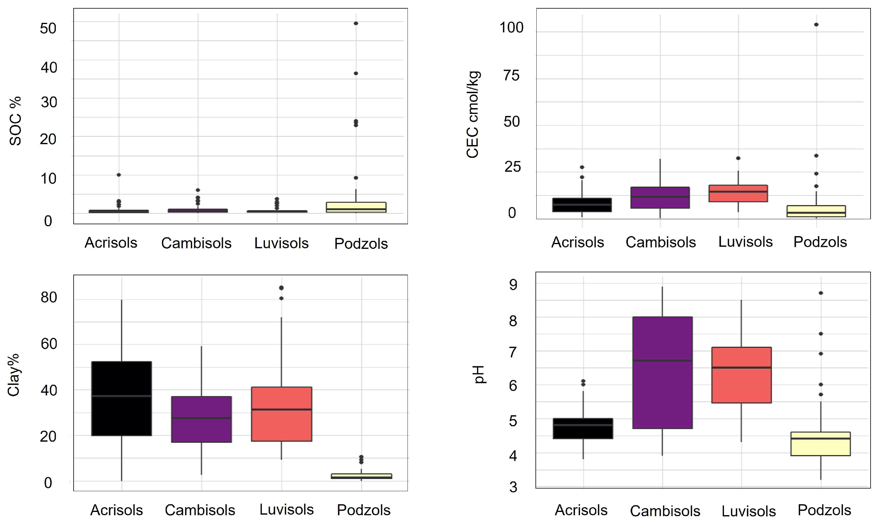
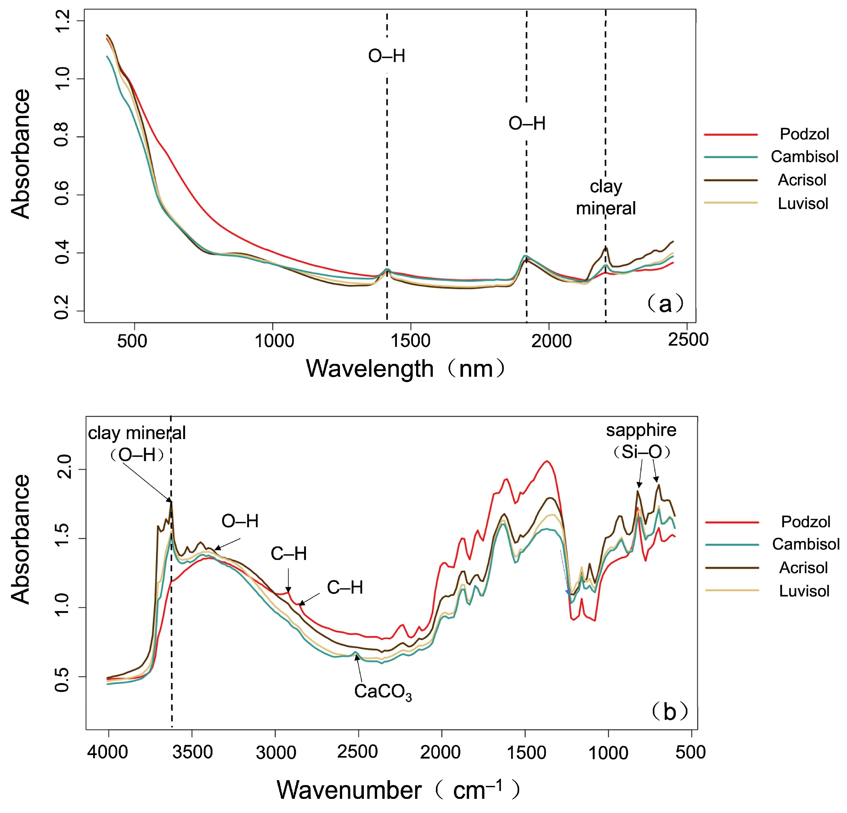
3.1. Soil Properties and Spectral Characteristic

The spectral response of soil is influenced by its physicochemical properties. These properties were selected based on their known influence on soil spectral signatures and their fundamental importance in determining soil classification. SOC significantly affects absorption in the vis–NIR region, where higher SOC content generally reduces reflectance. Clay minerals and carbonates strongly influence MIR spectral features. Cation exchange capacity (CEC) reflects the soil’s ability to retain and exchange nutrients and is closely associated with clay minerals and organic matter. Additionally, hydrogen (pH) affects various chemical reactions in soil that can alter their spectral response patterns. For instance, acidic soils such as Podzol are rich in iron oxides, which exhibit characteristic absorption in the vis–NIR bands.

Figure 3 illustrates the distinct characteristics of SOC, CEC, clay content, and pH across the four soil classes. Podzol, found in high-latitude, humid regions, is a typical acidic soil with a surface layer of dark-colored litter (O horizon) and a dark grey humus accumulation layer (A horizon). As a result, Podzol exhibits the highest median, interquartile range, and upper outlier variability in SOC, with a low pH value suggesting its strong acidity. But its clay content and CEC are the lowest, suggesting a coarse texture, such as sandy soil. Acrisol, though low in SOC, has the highest clay content. This can be attributed to its tropical environment, where intense rainfall accelerates mineral weathering and clay formation. Nutrients are leached to deeper layers, forming a well-developed clay horizon. The physicochemical properties of Cambisol and Luvisol are relatively similar, and both of their SOCs are low. However, Cambisol has the lowest SOC among the four soils, and its pH is closer to neutral. This can be explained by Cambisol’s early developmental stage, with limited horizon differentiation and minimal morphological changes, retaining characteristics of its parent material. Consequently, Cambisol has not undergone extensive weathering or mineral transformation, leading to lower clay content and CEC than Luvisol. In contrast, Luvisol has a higher clay content and relatively greater CEC.

Analyzing and comparing spectral characteristics involved calculation of the mean and standard deviation absorbance ranges for all samples’ vis–NIR and MIR spectra (Figure 4a). The absorbance of soil within the 400–1100 nm range exhibited a rapid decrease with increasing wavelength, forming an approximately straight line. The spectral curve exhibited higher absorbance values in the 400–600 nm range, with distinct absorption features at 410 nm, 570 nm, and 660 nm, primarily attributed to SOC and iron oxides. This observation aligns with previous studies, which indicate that spectral reflectance in the visible region increases with higher iron oxide content [43,44]. Additionally, organic matter exhibits absorption features across multiple vis–NIR spectral bands. Weak absorption peaks at 1000 nm were mainly due to hematite and clinopyroxene mineral absorption rich in iron. Prominent absorption peaks near 1400 nm and 1950 nm were primarily a result of water absorption, attributed to the stretching and bending vibrations of O–H functional groups in water molecules. The absorption features at 1900 nm and 2200 nm, attributed to clay minerals (e.g., kaolinite, montmorillonite, and illite), appear relatively weak.

Compared to vis–NIR, MIR spectroscopy (2500–25,000 nm) contained more sufficient soil information (Figure 4b). The MIR spectral region exhibited distinct peaks and troughs within the 4000–2000 cm⁻¹ range and numerous smaller amplitude peaks and troughs within the 2000–650 cm⁻¹ range. The 3616–3742 cm⁻¹ range primarily reflected the stretching bands of O–H groups in clay minerals such as kaolinite and montmorillonite [33]. Various organic compounds, clay minerals, and quartz exhibited notable peaks at specific wavenumbers (1080 cm⁻¹, 800 cm⁻¹, 780 cm⁻¹, and 700 cm⁻¹ for quartz; 1910 cm⁻¹, 1810 cm⁻¹, 1740 cm⁻¹, and 1710 cm⁻¹ for kaolinite and montmorillonite). These spectral features indicate that MIR spectroscopy exhibits a stronger response to clay minerals. Similar findings have been reported in previous studies, highlighting the superior performance of MIR spectroscopy in predicting soil properties such as pH, OC, CEC, and clay content [45,46].

Overall, these spectral patterns align with findings from previous research by Viscarra Rossel et al. [34] and Soriano-Disla et al. [47], who identified similar absorption features in global soil datasets. However, our analysis reveals some unique spectral characteristics in the four soil classes studied, particularly in the MIR region, where Podzols show distinctive patterns related to their high organic matter content. This is consistent with previous observations that MIR spectra are particularly sensitive to soil organic compounds and mineral composition [48].

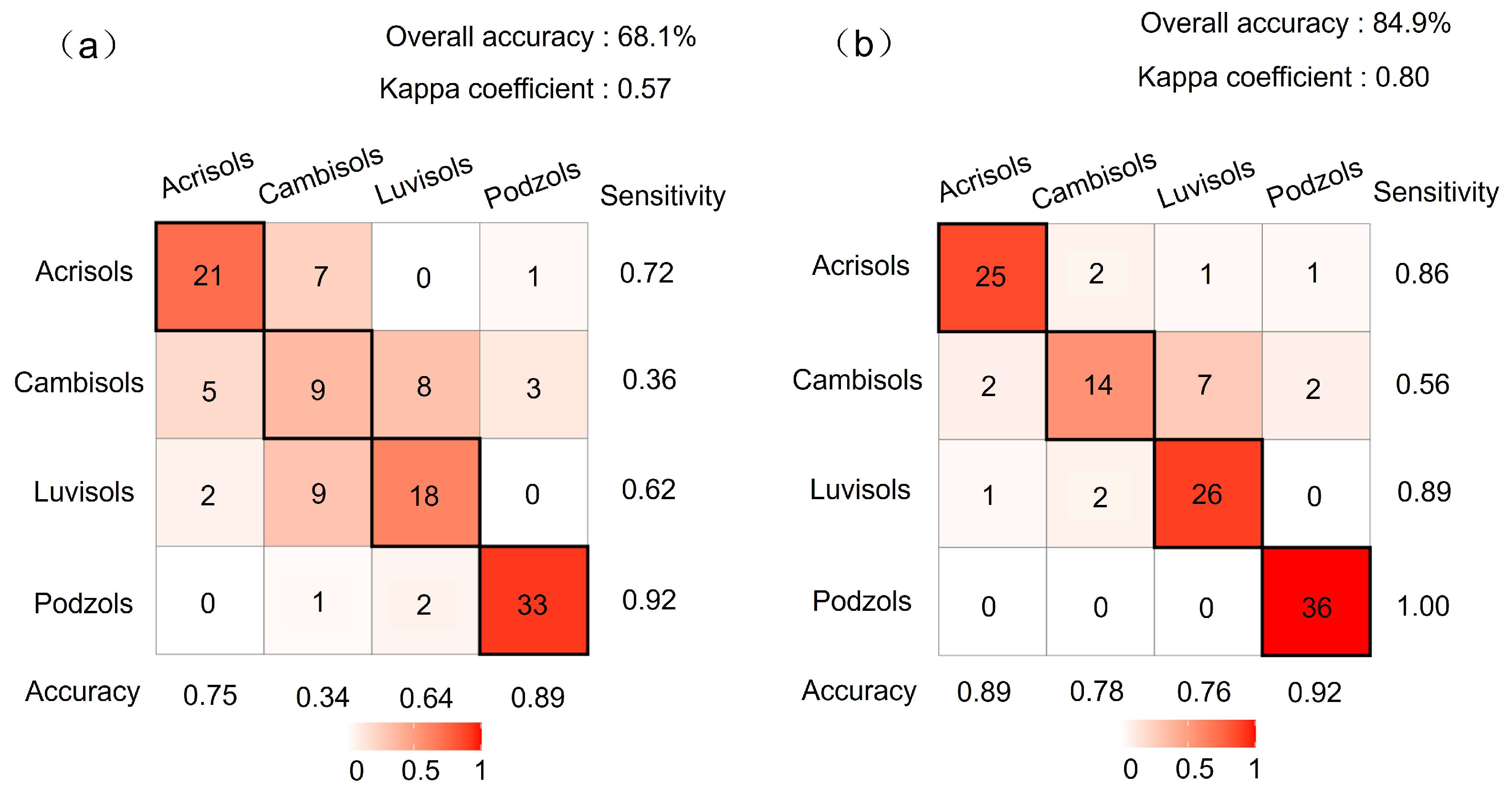
3.2. Classification Model Analyses Using Single Sensor

Figure 5 and Figure 6 show the modeling results of PLSDA and RF models based on vis–NIR and MIR spectra, respectively. Overall, the RF model yielded significantly higher classification accuracy than the PLSDA model. Across various soil samples, the RF model demonstrated improved classification accuracy for different soil classes. Podzols and Acrisols achieved high identification accuracy with both models, surpassing Luvisols and Cambisols. The prediction accuracy class for soil classes remained consistent for both vis–NIR and MIR spectra: Podzols > Acrisols > Luvisols > Cambisols. The RF model, especially the MIR spectrum, displayed superior predictive capability compared to the vis–NIR spectrum. Notably, Cambisols samples, which exhibited poor classification performance with vis–NIR, achieved over 80% correct classification with MIR-RF, demonstrating the best classification performance.

In summary, the MIR-RF model demonstrated the best performance, achieving an overall accuracy of 89.1% on the validation set with a Kappa coefficient of 0.85. Substantial improvements in overall classification accuracy were observed, with a 3.4% enhancement compared to vis–NIR-RF. Under the optimal MIR-RF model, Podzols exhibited the highest prediction accuracy (Sensitivity = 1, Accuracy = 0.97), followed by Acrisols (Sensitivity = 0.86, Accuracy = 0.93), while Cambisols and Luvisols displayed slightly lower prediction accuracy (Sensitivity < 0.86, Accuracy < 0.83).

3.3. Classification Model Analyses Using Sensor Fusion

3.3.1. Low-Level Fusion Predictions (SF1)

This study employed the first 20 principal components from the simple concatenated spectra as input. Figure 7 illustrates the results of low-level fusion. Although the model’s performance in predicting Podzols was inferior to single sensors, it achieved the best classification results among the four soil classes, with a sensitivity of 0.94 and an accuracy of 0.85. The RF model demonstrated an overall accuracy of 11.8%, higher than that of PLSDA. While the PLSDA model exhibited improved sensitivity and accuracy for Cambisols, it did not achieve the desired predictive performance.

Compared to the best predictive model of single sensors, SF1 did not significantly enhance the prediction of any of the four soil classes. The PLSDA model outperformed the vis–NIR model in classification performance but fell short of the MIR model. The overall classification accuracy of the SF1 spectral data improved by 8.4% compared to the vis–NIR-PLSDA model, with the Kappa coefficient increased by 0.11. However, the RF model for SF1 spectral data performed the worst, showing no improvement and even a decrease in predictive accuracy across the four soil classes. In contrast to the linear PLSDA model’s performance, the results failed to demonstrate the advantages of fusion techniques in the RF model. Therefore, the RF model based on MIR spectra exhibited the best classification accuracy (89.1%), suggesting that even with the inclusion of vis–NIR spectral information, the predictive performance of MIR spectra could not be surpassed.

3.3.2. Middle-Level Fusion Predictions (SF2)

Figure 8 presents the results of the two classification models using OPA to fuse vis–NIR and MIR data. The RF model outperformed the PLSDA model regarding overall classification accuracy, achieving 84.9% with a Kappa coefficient of 0.80. Compared to the PLSDA model, the RF model demonstrated superior accuracy across all four soil classes—Podzols, Luvisols, Cambisols, and Acrisols. Both models exhibited high accuracy in predicting Podzols and Acrisols but less satisfactory performance in predicting Cambisols and Luvisols.

Compared to SF1, the PLSDA model based on SF2 demonstrated lower overall classification accuracy, while the RF model’s accuracy increased by 2.5%. Relative to single-spectral models, the PLSDA model improved performance in the vis–NIR spectra, with an overall accuracy increase from 62.2% to 68.1%. However, this improvement did not match the performance level of MIR spectra, and no RF model achieved accuracy comparable to that of single-spectral classification models. The impact of OPA fusion on model accuracy was minimal, consistent with prior findings where OPA fusion failed to enhance the accuracy of PLSR models in predicting SOC and calcium (Ca) [49].

4. Discussion

4.1. Accuracy Comparison: Single Sensor vs. Sensor Fusion

The analysis of the single-sensor results (Figure 6 and Figure 7) in this study indicates that both the PLSDA and RF algorithms show that the MIR sensor outperforms the vis–NIR sensor. This finding is consistent with previous research [11,12,31]. The absorbance curves presented in Figure 4 reveal the differences between the two sensors regarding molecular vibrational frequencies and characteristics. Specifically, the vis–NIR absorbance curves exhibit smoother and more overlapping features, whereas the MIR absorbance curves demonstrate more pronounced fluctuations and variability. This suggests that the vibrational modes of molecular groups in the MIR region are more intense, leading to more distinct spectral absorption bands. This is primarily because fundamental vibrational frequencies of molecules are concentrated in the MIR region [50,51]. Consequently, vis–NIR has a lower sensitivity for estimating soil properties, while MIR spectroscopy provides more abundant information about soil composition, including clay minerals and quartz. Previous research has demonstrated that for most soil properties, the spectral specificity and intensity in the MIR region are significantly higher compared to the vis–NIR region. As a result, the predictive performance of MIR spectra tends to be more effective than vis–NIR or the combination of both [47,52,53]. Moreover, studies have shown that light scattering is much more pronounced in the NIR region than in the MIR, making NIR spectra more susceptible to scattering effects. Additionally, NIR spectra are more prone to instrumental errors than MIR, which can lead to greater prediction biases in NIR-based models than those relying on MIR spectra [48]. These findings further confirm the potential of MIR spectroscopy in soil classification.

Despite the fact that spectral fusion somewhat improves soil classification accuracy, in the PLSDA model, for instance, the classification capabilities of the SF1 and SF2 methods surpass those of the individual vis–NIR spectra but still fall short compared to the classification performance of the MIR spectra alone. Related studies have also found that low-level spectral fusion generally outperforms vis–NIR spectra for organic carbon prediction but is less effective than MIR spectra [44,54,55]. This indicates that low-level fusion can enhance the minimum accuracy of single spectra but may not improve their maximum accuracy, resulting in a trade-off between them. However, for some soil classes like Cambisols and Luvisols, the OPA method performed slightly worse than SF1. This suggests that although PCA reduced dimensionality, some components still mainly reflected noise or irrelevant information. Since RF is sensitive to such information, its accuracy easily drops when soil classes have similar mineral compositions and unclear boundaries [16].

In the RF model, the classification performance metrics (overall accuracy and Kappa coefficient) for all four spectral patterns outperform those of PLSDA. This is consistent with previous studies, which show that RF outperforms the linear PLSDA for predicting most soil parameters [56]. This advantage stems primarily from RF’s ability to model nonlinear relationships and effectively alleviate multicollinearity issues. PLSDA relies on linear projections to extract features, making it difficult to capture higher-order interactions between spectral features. In contrast, RF uses nonlinear decision tree splitting to delve deeper into spectral information without assuming linear relationships between variables [57]. The RF model all achieved over 80% accuracy, while PLSDA reached a maximum of only 71.4%. In four spectral modes, RF’s Kappa coefficient was on average 0.24 higher than that of PLSDA. The accuracy gap was largest based in the vis–NIR dataset, reaching 23.25%. Due to strong correlations between adjacent wavelengths, vis–NIR spectra suffer from severe multicollinearity. PLSDA reduces dimensionality using latent variables, but this approach may lead to the loss of important spectral information. In contrast, RF enhances model robustness through bootstrap sampling and reduces the influence of multicollinearity on classification using random feature selection (mtry), improving prediction reliability [41].

Across all spectral settings, RF consistently outperforms PLSDA. The RF model based on MIR spectra achieved the highest classification accuracy (overall accuracy = 89.1%, Kappa coefficient = 0.85), even surpassing spectral fusion models. In the RF model, SF1 and SF2 performed worse than the single-spectral model. Despite the theoretical advantages of spectral fusion, our results show limited improvement over MIR spectroscopy alone. In particular, the SF1 fusion method shows overall poorer classification performance. It keeps all the original vis–NIR and MIR information but does not remove redundancy and noise, which affects the model’s performance. For the limited improvement of the two fusion methods, on the one hand, MIR spectra already capture key features like organic matter, minerals, and carbonates. The addition of vis–NIR spectra causes a high overlap in feature responses, introducing redundancy and noise. On the other hand, combining less-informative spectral regions (vis–NIR) with more informative ones (MIR) can potentially reduce overall classification accuracy. If one spectral region (such as MIR) has already captured the key discriminative features for classification, adding a weakly related and less-informative region may introduce noise and dilute the advantage of MIR, thereby masking the original key features. Our study found that using MIR spectra alone already achieved a high classification accuracy (89.1%), so adding vis–NIR spectra did not significantly improve prediction performance. Instead, the redundancy introduced by vis–NIR spectra weakened the fusion model’s performance. Similar effects have been observed in previous several studies, where spectral fusion models sometimes performed worse than individual sensor models and even led to decreased prediction accuracy [58,59,60]. This suggests that the effectiveness of fusion is highly dependent on the relative information content of the combined spectral regions. In other words, merging MIR with vis–NIR spectra introduces redundant/noisy variables that outweigh potential benefits, particularly when MIR alone captures sufficient discriminative features [45].

Ultimately, in this study, the spectral fusion approach did not provide substantial benefits in enhancing model performance. In certain cases, as their synergy of fusion sensors is not always advantageous. Therefore, when employing data fusion techniques, it is essential to carefully consider potential sources of error that could affect prediction accuracy. In our study, the superior accuracy of the MIR-RF model highlights its effectiveness in providing detailed chemical information. However, MIR spectrometers—particularly benchtop models—are prohibitively expensive and require specialized maintenance, rendering them impractical for field deployment. Although portable devices like the Agilent 4200 exist, they are sensitive to sample preparation and environmental conditions, which reduces their convenience and efficiency [2]. In contrast, vis–NIR may offer a cost-effective alternative where slightly lower accuracy is acceptable.

4.2. Optimal Strategy for Four Soil Classes Determination

From the classification results of the four soil classes, Podzols were classified better than the other three soils in both spectral type and classification method and were classified best in MIR. The classification sensitivity of Podzols in the MIR–PLSDA model is 1, and the accuracy is 0.86; all samples were classified correctly, and there were six samples from Acrisols, Cambisols, and Luvisols incorrectly categorized as Podzols, with Cambisols accounting for 4 of them (Figure 6a). Because of the linear nature and overfitting of the entire spectrum in the model, spectral overlap between Cambisols and Podzols occurs, causing Cambisols to be misclassified as Podzols. The unique acidic characteristics of Podzols make them more stable in classification and less likely to be misclassified as Cambisols. The MIR-RF model (Figure 6b), through nonlinear processing and automatic weighting of key bands, better distinguishes between these two soil classes, reducing misclassification. So, all Podzol validation samples were accurately classified, with the model demonstrating the best performance in identifying Podzols, achieving a classification accuracy of 0.97.

Figure 3 illustrates that Podzols exhibit notably higher mean values, ranges, and variability in SOC compared to other soil classes. These attributes provide the model with more distinguishable information, particularly features related to soil organic matter (SOM). In the vis–NIR region (Figure 9a), the absorption spectral features of Podzols are significantly stronger than those of other soil classes. This spectral region is predominantly influenced by chromophores and organic matter content in the soil [34]. Meanwhile, at around 1400 nm, Podzols show a weak absorption peak. This band is a major water absorption region, influenced by adsorbed water on the soil surface and structural water in the O–H lattice of clay minerals, and it lacks the Al–OH clay mineral absorption feature near 2200 nm. This is attributed to the absence of abundant clay minerals and iron oxide spectral features in Podzols, which reflects the extensive leaching of metal cations such as calcium, potassium, magnesium, and sodium during the intense acidic weathering process typical of this soil class. Consequently, Podzols exhibit lower CEC and base saturation (Figure 3). As a result, the vis–NIR spectral curve of Podzols is relatively flat. Podzols show exceptional classification performance in the MIR spectrum, mainly due to MIR’s ability to sensitively detect the chemical components and characteristic spectral signals in Podzols, particularly organic matter. They display unique C–H absorption bands at 2930 cm⁻¹ in the MIR spectrum (Figure 9b), which are absent in other soils, distinguishing them from other soil classes. In the MIR range, spectral absorption features are more strongly correlated with soil organic matter content [53], which also explains the higher classification accuracy of Podzols in the MIR region. Overall, the distinct spectral characteristics of Podzols, especially within the MIR spectral range, significantly enhance the model’s classification capability.

The prediction accuracy of the Acrisols was second only to that of the Podzols, with the optimal prediction model being in the RF range. The accuracy and sensitivity in vis–NIR-RF and MIR-RF were the same for this soil class (Accuracy = 0.93, Sensitivity = 0.86), but MIR had 3.4% higher overall classification accuracy than vis–NIR. In the vis–NIR spectral range (Figure 9a), the Acrisols showed a distinct clay mineral absorption band at 2200 nm; within the MIR spectral range (Figure 9b), there were strong absorption peaks and valleys near 3600 cm⁻¹, which were associated with the strongest clay mineral absorption band, and there were distinct absorption bands of Si–O near 690 cm⁻¹ and 820 cm⁻¹. In the quantitative analysis of clay content, the spectral bands at 516 nm, 880 nm, and 2204 nm have significant weight in determining clay concentration [47]. As the clay content in the soil increases, the spectral sensitivity to these minerals also becomes more pronounced. This characteristic explains the strong predictive performance of Acrisol soils in the model. The high clay content of Acrisols allows the model to more accurately capture their spectral features. However, Luvisols, which have the second-highest clay content after Acrisols (Figure 3), are sometimes misclassified as other high-clay soils. For Cambisols, although they are less developed and experience weaker nutrient leaching, they may, in some cases, still contain clay illuviation horizons. These horizons can exhibit spectral similarities to the argillic horizon found in Acrisols. If the model mistakenly interprets the clay illuviation layer in Cambisols as a fully developed argillic horizon, it could lead to the misclassification of Cambisols as Acrisols. Overall, the developmental state of the clay horizons and the spectral similarities between soil classes are key factors contributing to these classification errors.

The classification accuracies of Luvisols and Cambisols were lower than the other two. In the SF2 method, the former had the best classification with an accuracy of 0.76 and a sensitivity of 0.89, and the best classification result for Cambisols was an accuracy of 0.83 and a sensitivity of 0.80. Among these, the highest rate of misclassification occurred with Luvisols. From the average spectral curves (Figure 9), both have similar spectral characteristics in the vis–NIR and MIR spectral ranges; from the distribution of sampling points (Figure 1), the sampling points are spatially close to each other, with a certain degree of overlap, and similar soil development environments mean that the physical and chemical traits of the different soil types have similarities, which somewhat explains the phenomenon of confusion and misclassification of the two soils in the classification model. These factors can help explain the confusion and misclassification between the two types in the classification model. In the MIR region around the 2550 cm⁻¹ band (Figure 9b), there were small absorption bands in both of the high-leaching soils, which show the absorption characteristics of the sedimentary layer and the parent layer and are mainly influenced by soil CaCO₃.

Cambisols performed the worst among of the four soil classification results, and only slightly better in the MIR-RF model. Cambisols achieved more than 80% correct MIR-RF model classification. Still, five samples were classified as Luvisols (four samples) and Acrisols (one sample), and four samples from Luvisols (three samples) and Acrisols (one sample) were classified in the fledgling soil group. The organic carbon content in Cambisol is the lowest among the four soil classes studied (Figure 3). This lower content indicates less organic matter accumulation, resulting in a less-stable soil structure compared to more developed soil classes. The weak organic matter features in the Cambisol spectrum make it less distinct compared to other soil classes, complicating accurate classification by models. Luvisols usually have a distinct argillic B horizon, showing clay mineral absorption features at 1400 nm, 1900 nm, 2200 nm, and 3645 cm⁻¹. These bands are highly overlapped with the spectra of Cambisols. In addition, the two soils have similar organic matter content and carbonate levels in some areas, which makes them difficult to separate in the vis–NIR region due to broad, overlapping absorption bands. Although MIR improves their separability with clearer and more specific absorption peaks, some misclassification still occurs, especially in transitional or mixed parent material soil profiles. As a result, when distinguishing Cambisols from other soils, models struggle to utilize effective spectral features, leading to poorer classification performance. This lack of clear spectral characteristics increases the likelihood of confusing Cambisols with other soils that have similar mineral properties but different organic matter content, thereby adding to the classification difficulty.

To improve the discrimination between these similar soil classes, future research could explore advanced spectral preprocessing techniques to reduce noise further or to enhance the signals, or both (e.g., multiplicative scatter correction, standard normal variate transformation) [13]. Alternatively, integrating auxiliary environmental variables such as topographic attributes, climate data, or soil moisture could provide additional discriminatory ability beyond spectral information. More targeted sampling strategies focusing on diagnostic horizons rather than whole profiles might also improve classification accuracy for these challenging soil classes by capturing key pedogenic features and minimizing classification ambiguities.

4.3. Future Prospects

This study utilizes spectral data to extract soil property information, providing essential support for soil classes identification. In particular, vis–NIR and MIR spectroscopy have demonstrated strong capabilities in predicting SOM, clay content, and iron oxides [45,61,62]. However, these predictions do not fully capture the unique characteristics of each soil class. When soil samples exhibit similar physical and chemical properties, the analysis may become overly mechanistic, and insufficient information could lead to confusion and misclassification. To further enhance soil classification accuracy, hyperspectral imaging (HSI) may provide a novel perspective. By combining spectral data with spatial information [63,64], HSI offers richer discriminatory information, which can potentially improve the identification of complex soil types. Moreover, combining HSI with vis–NIR and MIR spectroscopy may leverage the complementary advantages of different spectral ranges, enhancing soil characterization and classification. However, its effectiveness requires further validation across distinct soil types, environments, and data fusion strategies.

This study confirms the significant advantage of MIR spectroscopy in soil classification on a broader scale, but its application in the field is limited due to the high cost of equipment, sensitivity to environmental conditions, and operational complexity. In future research, integrating multi-sensor monitoring with Artificial Intelligence (AI) algorithms, and combining soil science knowledge [65], including soil moisture, particle size, and other information from diagnostic horizons, can dynamically correct environmental interference in MIR data, improving its stability and practicality in field applications. These improvements will not only enhance the accuracy of single-point measurements but also help optimize soil management strategies. Currently, agricultural management relies on portable devices like vis–NIR, with MIR serving as a high-precision reference for calibration. As multi-sensor fusion technology advances, field soil monitoring is expected to evolve from single-sensor systems to multi-mode, collaborative systems, supporting more precise agricultural decision-making.

5. Conclusions

In this study, we compared the capabilities of single sensors and sensor fusion in soil classification using the PLSDA and RF algorithms. This not only deepens the theoretical understanding of spectral data classification capabilities but also offers practical insights for improving soil classification accuracy in varied contexts, thereby supporting sustainable agricultural management and soil resource utilization worldwide. The findings are summarized as follows:

(1)

RF outperforms PLSDA: The RF model outperforms the PLSDA model in soil classification. By integrating multiple decision trees, RF captures more detailed soil information and achieves better classification accuracy than the linear PLSDA model.

(2)

MIR-RF achieves optimal accuracy: The MIR-RF model reaches the highest classification accuracy of 89.1%, demonstrating the superior information content of MIR spectra for soil discrimination. While fused spectra offers slight accuracy gains over vis–NIR spectra in the RF model, the fusion methods do not surpass the performance of the single MIR spectrum, suggesting that MIR spectroscopy captures the most essential soil classification information.

(3)

Soil-specific performance patterns: The MIR spectrum performs well for classifying Podzols and Acrisols due to their distinctive organic matter and clay mineral features. However, neither single sensors nor fusion models effectively classify Luvisols and Cambisols with the same accuracy, highlighting the need for specialized approaches when dealing with spectrally similar soil classes.

References

1. Monger, C.; Michéli, E.; Aburto, F.; Itkin, D. Soil classification as a tool for contributing to sustainability at the landscape scale and forecasting impacts of management practices in agriculture and forestry. Soil Tillage Res. 2024, 244, 106216. [Google Scholar] [CrossRef]
2. Li, S.; Viscarra Rossel, R.A.; Webster, R. The cost-effectiveness of reflectance spectroscopy for estimating soil organic carbon. Eur. J. Soil Sci. 2022, 73, e13202. [Google Scholar] [CrossRef]
3. Hong, Y.; Sanderman, J.; Hengl, T.; Chen, S.; Wang, N.; Xue, J.; Zhuo, Z.; Peng, J.; Li, S.; Chen, Y.; et al. Potential of globally distributed topsoil mid-infrared spectral library for organic carbon estimation. Catena 2024, 235, 107628. [Google Scholar] [CrossRef]
4. Nawar, S.; Abdul Munnaf, M.; Mouazen, A.M. Machine learning based on-line prediction of soil organic carbon after removal of soil moisture effect. Remote Sens. 2020, 12, 1308. [Google Scholar] [CrossRef]
5. Ahmadi, A.; Emami, M.; Daccache, A.; He, L. Soil properties prediction for precision agriculture using visible and near-infrared spectroscopy: A systematic review and meta-analysis. Agronomy 2021, 11, 433. [Google Scholar] [CrossRef]
6. Yin, J.; Shi, Z.; Li, B.; Sun, F.; Miao, T.; Shi, Z.; Chen, S.; Yang, M.; Ji, W. Prediction of soil properties in a field in typical black soil areas using in situ MIR spectra and its comparison with vis–NIR spectra. Remote Sens. 2023, 15, 2053. [Google Scholar] [CrossRef]
7. Shi, Z.; Wang, Q.; Peng, J.; Ji, W.; Liu, H.; Li, X.; Viscarra Rossel, R.A. Development of a national VNIR soil-spectral library for soil classification and prediction of organic matter concentrations. Sci. China Earth Sci. 2014, 57, 1671–1680. [Google Scholar] [CrossRef]
8. Chen, S.; Li, S.; Ma, W.; Ji, W.; Xu, D.; Shi, Z.; Zhang, G. Rapid determination of soil classes in soil profiles using vis–NIR spectroscopy and multiple objectives mixed support vector classification. Eur. J. Soil Sci. 2019, 70, 42–53. [Google Scholar] [CrossRef]
9. Vasques, G.M.; Demattê, J.A.M.; Viscarra Rossel, R.A.; Ramírez-López, L.; Terra, F.S. Soil classification using visible/near-infrared diffuse reflectance spectra from multiple depths. Geoderma 2014, 223, 73–78. [Google Scholar] [CrossRef]
10. Xie, X.L.; Li, A.B. Identification of soil profile classes using depth-weighted visible–near-infrared spectral reflectance. Geoderma 2018, 325, 90–101. [Google Scholar] [CrossRef]
11. Afriyie, E.; Verdoodt, A.; Mouazen, A.M. Data fusion of visible near-infrared and mid-infrared spectroscopy for rapid estimation of soil aggregate stability indices. Comput. Electron. Agric. 2021, 187, 106229. [Google Scholar] [CrossRef]
12. Shi, Z.; Yin, J.; Li, B.; Sun, F.; Miao, T.; Cao, Y.; Shi, Z.; Chen, S.; Hu, B.; Ji, W.; et al. Comparison of depth-specific prediction of soil properties: MIR vs. vis–NIR spectroscopy. Sensors 2023, 23, 5967. [Google Scholar] [CrossRef] [PubMed]
13. Li, S.; Shi, Z.; Chen, S.; Ji, W.; Zhou, L.; Yu, W.; Webster, R. In situ measurements of organic carbon in soil profiles using vis–NIR spectroscopy on the Qinghai–Tibet plateau. Environ. Sci. Technol. 2015, 49, 4980–4987. [Google Scholar] [CrossRef]
14. Hutengs, C.; Seidel, M.; Oertel, F.; Ludwig, B.; Vohland, M. In situ and laboratory soil spectroscopy with portable visible-to-near-infrared and mid-infrared instruments for the assessment of organic carbon in soils. Geoderma 2019, 355, 113900. [Google Scholar] [CrossRef]
15. Linker, R. Soil classification via mid-infrared spectroscopy. Comput. Comput. Technol. Agric. 2008, 259, 1137–1146. [Google Scholar]
16. Zhang, Y.; Hartemink, A.E.; Huang, J. Spectral signatures of soil horizons and soil orders–An exploratory study of 270 soil profiles. Geoderma 2021, 389, 114961. [Google Scholar] [CrossRef]
17. Amundson, R.; Berhe, A.A.; Hopmans, J.W.; Olson, C.; Sztein, A.E.; Sparks, D.L. Soil and human security in the 21st century. Science 2015, 348, 1261071. [Google Scholar] [CrossRef]
18. Guerra, C.A.; Bardgett, R.D.; Caon, L.; Crowther, T.W.; Delgado-Baquerizo, M.; Montanarella, L.; Navarro, L.M.; Orgiazzi, A.; Singh, B.K.; Tedersoo, L. Tracking, targeting, and conserving soil biodiversity. Science 2021, 371, 239–241. [Google Scholar] [CrossRef]
19. Ng, W.; Minasny, B.; Montazerolghaem, M.; Padarian, J.; Ferguson, R.; Bailey, S.; McBratney, A.B. Convolutional neural network for simultaneous prediction of several soil properties using visible/near-infrared, mid-infrared, and their combined spectra. Geoderma 2019, 352, 251–267. [Google Scholar] [CrossRef]
20. Grunwald, S.; Vasques, G.M.; Rivero, R.G. Fusion of soil and remote sensing data to model soil properties. Adv. Agron. 2015, 131, 1–109. [Google Scholar]
21. Veum, K.S.; Sudduth, K.A.; Kremer, R.J.; Kitchen, N.R. Sensor data fusion for soil health assessment. Geoderma 2017, 305, 53–61. [Google Scholar] [CrossRef]
22. Hall, D.L.; Llinas, J. An introduction to multisensor data fusion. Proc. IEEE 1997, 85, 6–23. [Google Scholar] [CrossRef]
23. Barros, A.S.; Safar, M.; Devaux, M.F.; Robert, P.; Bertrand, D.; Rutledge, D.N. Relations between mid-infrared and near-infrared spectra detected by analysis of variance of an intervariable data matrix. Appl. Spectrosc. 1997, 51, 1384–1393. [Google Scholar] [CrossRef]
24. Terra, F.S.; Rossel, R.A.V.; Demattê, J.A.M. Spectral fusion by Outer Product Analysis (OPA) to improve predictions of soil organic C. Geoderma 2019, 335, 35–46. [Google Scholar] [CrossRef]
25. Jaillais, B.; Ottenhof, M.A.; Farhat, I.A.; Rutledge, D.N. Outer-product analysis (OPA) using PLS regression to study the retrogradation of starch. Vib. Spectrosc. 2006, 40, 10–19. [Google Scholar] [CrossRef]
26. Bai, Y.; Yang, W.; Wang, Z.; Cao, Y.; Li, M. Improving the estimation accuracy of soil organic matter based on the fusion of near-infrared and Raman spectroscopy using the outer-product analysis. Comput. Electron. Agric. 2024, 219, 108760. [Google Scholar] [CrossRef]
27. Hong, Y.; Chen, S.; Hu, B.; Wang, N.; Xue, J.; Zhuo, Z.; Yang, Y.; Chen, Y.; Peng, J.; Liu, Y.; et al. Spectral fusion modeling for soil organic carbon by a parallel input-convolutional neural network. Geoderma 2023, 437, 116584. [Google Scholar] [CrossRef]
28. Li, X.; Pan, W.; Li, D.; Gao, W.; Zeng, R.; Zheng, G.; Cai, K.; Zeng, Y.; Jiang, C. Can fusion of vis–NIR and MIR spectra at three levels improve the prediction accuracy of soil nutrients? Geoderma 2024, 441, 116754. [Google Scholar] [CrossRef]
29. Ji, W.; Adamchuk, V.I.; Chen, S.; Su, A.S.M.; Ismail, A.; Gan, Q.; Shi, Z.; Biswas, A. Simultaneous measurement of multiple soil properties through proximal sensor data fusion: A case study. Geoderma 2019, 341, 111–128. [Google Scholar] [CrossRef]
30. Zhang, Y.; Hartemink, A.E. Data fusion of vis–NIR and PXRF spectra to predict soil physical and chemical properties. Eur. J. Soil Sci. 2020, 71, 316–333. [Google Scholar] [CrossRef]
31. Xu, H.; Xu, D.; Chen, S.; Ma, W.; Shi, Z. Rapid determination of soil class based on visible-near infrared, mid-infrared spectroscopy and data fusion. Remote Sens. 2020, 12, 1512. [Google Scholar] [CrossRef]
32. Xu, D.; Chen, S.; Viscarra Rossel, R.A.; Biswas, A.; Li, S.; Zhou, Y.; Shi, Z. X-ray fluorescence and visible near infrared sensor fusion for predicting soil chromium content. Geoderma 2019, 352, 61–69. [Google Scholar] [CrossRef]
33. Tavares, T.R.; Molin, J.P.; Javadi, S.H.; de Carvalho, H.W.P.; Mouazen, A.M. Combined use of vis-NIR and XRF sensors for tropical soil fertility analysis: Assessing different data fusion approaches. Sensors 2020, 21, 148. [Google Scholar] [CrossRef] [PubMed]
34. Viscarra Rossel, R.A.; Behrens, T.; Ben-Dor, E.; Brown, D.J.; Demattê, J.A.M.; Shepherd, K.D.; Shi, Z.; Stenberg, B.; Stevens, A.; Adamchuk, V.; et al. A global spectral library to characterize the world’s soil. Earth-Sci. Rev. 2016, 155, 198–230. [Google Scholar] [CrossRef]
35. Terhoeven-Urselmans, T.; Vagen, T.G.; Spaargaren, O.; Shepherd, K.D. Prediction of soil fertility properties from a globally distributed soil mid-infrared spectral library. Soil Sci. Soc. Am. J. 2010, 74, 1792–1799. [Google Scholar] [CrossRef]
36. Savitzky, A.; Golay, M.J.E. Smoothing and differentiation of data by simplified least squares procedures. Anal. Chem. 1964, 36, 1627–1639. [Google Scholar] [CrossRef]
37. Barker, M.; Rayens, W. Partial least squares for discrimination. J. Chemom. 2003, 17, 166–173. [Google Scholar] [CrossRef]
38. Brereton, R.G.; Lloyd, G.R. Support vector machines for classification and regression. Analyst 2010, 135, 230–267. [Google Scholar] [CrossRef]
39. Lee, L.C.; Liong, C.Y.; Jemain, A.A. Partial least squares-discriminant analysis (PLS-DA) for classification of high-dimensional (HD) data: A review of contemporary practice strategies and knowledge gaps. Analyst 2018, 143, 3526–3539. [Google Scholar] [CrossRef]
40. Breiman, L. Random forest. Mar. Learn. 2001, 45, 5–32. [Google Scholar] [CrossRef]
41. Liaw, A.; Wiener, M. Classification and regression by randomForest. R News 2002, 2, 18–22. [Google Scholar]
42. Kraemer, H.C. Extension of the kappa coefficient. Biometrics 1980, 36, 207–216. [Google Scholar] [CrossRef] [PubMed]
43. Viscarra, R.A.; Behrens, T. Using data mining to model and interpret soil diffuse reflectance spectra. Geoderma 2010, 158, 46–54. [Google Scholar]
44. Meng, X.; Yu, L.; Zhou, Y.; Li, S. Predicting organic carbon using data fusion of visible near-infrared and middle infrared spectra by proximal soil sensing. Chin. J. Soil Sci. 2022, 53, 301–307. [Google Scholar]
45. Viscarra Rossel, R.A.; Walvoort, D.J.J.; McBratney, A.B.; Janik, L.J.; Skjemstad, J.O. Visible, near infrared, mid infrared or combined diffuse reflectance spectroscopy for simultaneous assessment of various soil properties. Geoderma 2006, 131, 59–75. [Google Scholar] [CrossRef]
46. Coblinski, J.A.; Giasson, É.; Demattê, J.A.M.; Dotto, A.C.; Costa, J.J.F.; Vašát, R. Prediction of Soil Texture Classes through Different Wavelength Regions of Reflectance Spectroscopy at Various Soil Depths. Catena 2020, 189, 104485. [Google Scholar] [CrossRef]
47. Soriano-Disla, J.M.; Janik, L.J.; Viscarra Rossel, R.A.; Macdonald, L.M.; McLaughlin, M.J. The performance of visible, near-, and mid-infrared reflectance spectroscopy for prediction of soil physical, chemical, and biological properties. Appl. Spectrosc. Rev. 2014, 49, 139–186. [Google Scholar] [CrossRef]
48. Bellon-Maurel, V.; McBratney, A. Near-infrared (NIR) and mid-infrared (MIR) spectroscopic techniques for assessing the amount of carbon stock in soils—Critical review and research perspectives. Soil Biol. Biochem. 2011, 43, 1398–1410. [Google Scholar] [CrossRef]
49. Javadi, S.H.; Mouazen, A.M. Data fusion of XRF and vis–NIR using outer product analysis, granger–ramanathan, and least squares for prediction of key soil attributes. Remote Sens. 2021, 13, 2023. [Google Scholar] [CrossRef]
50. Nocita, M.; Stevens, A.; van Wesemael, B.; Aitkenhead, M.; Bachmann, M.; Barthes, B.; Gholizadeh, A.; Lobsey, C. Soil spectroscopy: An alternative to wet chemistry for soil monitoring. Adv. Agron. 2015, 132, 139–159. [Google Scholar]
51. Afriyie, E.; Verdoodt, A.; Mouazen, A.M. Estimation of aggregate stability of some soils in the loam belt of belgium using mid-infrared spectroscopy. Sci. Total Environ. 2020, 744, 140727. [Google Scholar] [CrossRef]
52. Stenberg, B.; Rossel, R.A.V.; Mouazen, A.M.; Wetterlind, J. Visible and near infrared spectroscopy in soil science. Adv. Agron. 2010, 107, 163–215. [Google Scholar]
53. Vohland, M.; Ludwig, M.; Thiele-Bruhn, S.; Hutengs, C. Determination of soil properties with visible to near- and mid-infrared spectroscopy: Effects of spectral variable selection. Geoderma 2014, 223, 88–96. [Google Scholar] [CrossRef]
54. Knox, N.M.; Grunwald, S.; McDowell, M.L.; Bruland, G.L.; Myers, D.B.; Harris, W.G. Modelling soil carbon fractions with visible near-infrared (VNIR) and mid-infrared (MIR) spectroscopy. Geoderma 2015, 239, 229–239. [Google Scholar] [CrossRef]
55. Greenberg, I.; Seidel, M.; Vohland, M.; Ludwig, B. Performance of field-scale lab vs in situ visible/near- and mid-infrared spectroscopy for estimation of soil properties. Eur. J. Soil Sci. 2022, 73, e13180. [Google Scholar] [CrossRef]
56. Xu, S.; Zhao, Y.; Wang, M.; Shi, X. A Comparison of Machine Learning Algorithms for Mapping Soil Iron Parameters Indicative of Pedogenic Processes by Hyperspectral Imaging of Intact Soil Profiles. Eur. J. Soil Sci. 2022, 73, e13204. [Google Scholar] [CrossRef]
57. de Santana, F.B.; Daly, K. A comparative study of MIR and NIR spectral models using ball-milled and sieved soil for the prediction of a range of soil physical and chemical parameters. Spectrochim. Acta Part A Mol. Biomol. Spectrosc. 2022, 279, 121441. [Google Scholar] [CrossRef]
58. Xu, D.; Zhao, R.; Li, S.; Chen, S.; Jiang, Q.; Zhou, L.; Shi, Z. Multi-sensor fusion for the determination of several soil properties in the Yangtze River Delta, China. Eur. J. Soil Sci. 2019, 70, 162–173. [Google Scholar] [CrossRef]
59. Hong, Y.; Munnaf, M.A.; Guerrero, A.; Chen, S.; Liu, Y.; Shi, Z.; Mouazen, A.M. Fusion of visible-to-near-infrared and mid-infrared spectroscopy to estimate soil organic carbon. Soil Tillage Res. 2022, 217, 105284. [Google Scholar] [CrossRef]
60. Xue, J.; Zhang, X.; Chen, S.; Lu, R.; Wang, Z.; Wang, N.; Hong, Y.; Chen, X.; Xiao, Y.; Ma, Y.; et al. The validity domain of sensor fusion in sensing soil quality indicators. Geoderma 2023, 438, 116657. [Google Scholar] [CrossRef]
61. Terra, F.S.; Dematte, J.A.M.; Viscarra Rossel, R.A. Proximal spectral sensing in pedological assessments: Vis–NIR spectra for soil classification based on weathering and pedogenesis. Geoderma 2018, 318, 123–136. [Google Scholar] [CrossRef]
62. Xu, D.; Ma, W.; Chen, S.; Jiang, Q.; He, K.; Shi, Z. Assessment of important soil properties related to Chinese Soil Taxonomy based on vis–NIR reflectance spectroscopy. Comput. Electron. Agric. 2018, 144, 1–8. [Google Scholar] [CrossRef]
63. Steffens, M.; Buddenbaum, H. Laboratory imaging spectroscopy of a stagnic luvisol profile—High resolution soil characterisation, classification and mapping of elemental concentrations. Geoderma 2013, 195, 122–132. [Google Scholar] [CrossRef]
64. Zhou, Y.; Biswas, A.; Hong, Y.; Chen, S.; Hu, B.; Shi, Z.; Guo, Y.; Li, S. Enhancing soil profile analysis with soil spectral libraries and laboratory hyperspectral imaging. Geoderma 2024, 450, 117036. [Google Scholar] [CrossRef]
65. Minasny, B.; McBratney, A.B. Machine Learning and Artificial Intelligence Applications in Soil Science. Eur. J. Soil Sci. 2025, 76, e70093. [Google Scholar] [CrossRef]
Figure 1. Map of the distribution of the 60 profiles in the global soil spectral library.
Remotesensing 17 01524 g001
Figure 3. Box plots of the main soil physicochemical properties of the selected samples.
Remotesensing 17 01524 g003
Figure 4. Mean absorbance curves and standard deviation ranges of vis–NIR (a) and MIR (b) spectra.
Remotesensing 17 01524 g004
Figure 5. Confusion matrix of soil classification based on vis–NIR spectra: PLSDA (a) vs. RF (b).
Remotesensing 17 01524 g005
Figure 6. Confusion matrix of soil classification based on MIR spectra: PLSDA (a) vs. RF (b).
Remotesensing 17 01524 g006
Figure 7. Confusion matrix of soil classification based on direct combination: PLSDA (a) vs. RF (b).
Remotesensing 17 01524 g007
Figure 8. Confusion matrix of soil classification based on outer product analysis: PLSDA (a) vs. RF (b).
Remotesensing 17 01524 g008
Figure 9. Average spectral curves of vis–NIR (a) and MIR (b) for soil profiles.
Remotesensing 17 01524 g009