Semi-Automatic Extraction of Hedgerows from High-Resolution Satellite Imagery

Abstract

Small landscape elements are critical in ecological systems, encompassing vegetated and non-vegetated features. As vegetated elements, hedgerows contribute significantly to biodiversity conservation, erosion protection, and wind speed reduction within agroecosystems. This study focuses on the semi-automatic extraction of hedgerows by applying the Object-Based Image Analysis (OBIA) approach to two multispectral satellite datasets. Multitemporal image data from PlanetScope and Copernicus Sentinel-2 have been used to test the applicability of the proposed approach for detailed land cover mapping, with an emphasis on extracting Small Woody Elements. This study demonstrates significant results in classifying and extracting hedgerows, a smaller landscape element, from both Sentinel-2 and PlanetScope images. A good overall accuracy (OA) was obtained using PlanetScope data (OA = 95%) and Sentinel-2 data (OA = 85%), despite the coarser resolution of the latter. This will undoubtedly demonstrate the effectiveness of the OBIA approach in leveraging freely available image data for detailed land cover mapping, particularly in identifying and classifying hedgerows, thus supporting biodiversity conservation and ecological infrastructure enhancement.

1. Introduction

Small Woody Elements (SWEs), including linear features such as hedgerows, tree lines, small woods, and riparian vegetation, are vital components of ecological systems. These features, located primarily outside forested areas, form a mosaic of interconnected ecosystem resources, significantly influencing landscape patterns [1]. Their ecological importance goes beyond their spatial extent, as they contribute to connectivity and biodiversity conservation by mitigating habitat fragmentation and enhancing structural complexity [2]. Beyond ecological functions, SWEs provide essential ecosystem services, including carbon sequestration, water filtration, erosion control, and microclimate regulation [3,4,5].

The multifunctionality of hedgerows, encompassing their capacity to provide multiple ecological, socio-economic, and cultural functions [6], must be carefully considered, especially at a local scale, where the management, structure, and composition of vegetation layer significantly influence hedgerow biodiversity and ecological functioning [7]. Agricultural intensification, urban development, and habitat fragmentation have led to a simplification of landscape structures [8]. To counteract these effects, implementing green landscape features, such as hedgerows, line trees, and other SWEs, is essential for preserving biodiversity and maintaining the ecosystem services they support [9,10].

European policy strongly supports the increase and conservation of SWEs. The Common Agricultural Policy emphasizes the importance of landscape elements in maintaining biodiversity and ecosystem services. Moreover, the European Union Biodiversity Strategy for 2030 aims to ensure a coherent Trans-European Nature Network (Natura 2000). This includes, for example, restoring high-diversity landscape features, such as buffer strips, fallow land, and hedgerows outside protected areas. The overarching objective of the strategy is to transform at least 10% of agricultural land into high-diversity landscape features to provide space for wild animals, plants, pollinators, and natural pest regulators [11]. Furthermore, the Nature Restoration Law (NRL) (EU Regulation 2024–1991 Regulation-EU-2024/1991-EN-EUR-Lex) mandates that countries implement measures to achieve a national upward trend in at least two of three indicators for agricultural ecosystems, one being the percentage of agricultural land featuring landscape elements with high biodiversity, such as hedgerows [11]. The NRL also emphasizes the protection of landscape features with high biodiversity, such as hedgerows, from negative external disturbances to ensure safe habitats and support biodiversity. Understanding the distribution, extent, and condition of SWEs within landscape ecology and biodiversity conservation is fundamental for guiding effective conservation efforts across different spatial scales [12]. As for forests, the timely and precise monitoring and mapping of cover is a vital aspect of sustainable management and the monitoring of ecosystem transformations [13,14]. In addition, accurate mapping of SWEs is important to achieving the objectives of outcome indicator I.10/C21 of the Common Agricultural Policy [15]: “Improved provision of ecosystem services: Proportion of agricultural land covered by landscape features”. This indicator aims to estimate the proportion of agricultural land covered by different landscape features, including linear features such as hedgerows, tree patches, forests, wetlands, and semi-natural areas such as field margins. The indicator has two components: the proportion of agricultural land covered by landscape features and a more detailed index of the structure of landscape elements [16].

Maps of SWEs are also useful tools to support biodiversity studies. Hedgerows play a critical role in providing food resources for wildlife, serving as habitats for important species like pollinators and resident and overwintering birds [17]. As highlighted by Hinsley et al. [18] in their study across the UK, hedgerow size and the presence of trees were found to positively influence bird species richness and abundance. In this regard, reliable maps of such landscape elements can support the design of more efficient sampling schemes. Moreover, spatially explicit information can be potentially included in decision support systems at a regional scale [19,20], thus supporting local and regional planning aimed at nature conservation. For instance, accurate identification of hedgerows enables the mapping of agricultural areas that require restoration measures, identifying where hedgerows have been destroyed or lost, and facilitating the implementation of ecological corridors [21].

In recent years, remote sensing has emerged as a valuable tool for accurately and efficiently mapping small landscape features. Initially, high-resolution multispectral imagery facilitated mapping through visual interpretation and extensive fieldwork, a time-consuming and labor-intensive process [22]. However, advancements in remote sensing technology have led to the development of automated methods for delineating vegetation elements, enhancing objectivity, and reducing time and resource demands [23]. Consequently, remote sensing approaches offer several advantages: repeatability, wide area coverage, and real-time accessibility.

Several factors influence the successful extraction of SWEs. Due to their shape and size, medium spatial resolution imagery may be insufficient to distinguish individual elements, leading to mixed pixels. Mixed pixels represent situations where hedgerows are interspersed with other landscape features or land cover types. To ensure consistent and accurate extraction, the features must be significantly larger than the spatial resolution of the imagery. Coarse-scale multispectral images complicate the identification and drawing of hedgerow boundaries, with factors such as the length-to-width ratio and the area of the feature influencing extraction accuracy. Consequently, low spatial resolution can lead to a reduction in classification accuracy [24].

Remote sensing techniques for SWE mapping vary based on resolution, ranging from MODIS-based tree cover assessments at low resolution to object-based classifications and pixel-swapping techniques at medium resolution [25,26]. Later approaches introduced automated feature extraction using Object-Based Image Analysis (OBIA) and machine learning [27,28,29]. In the context of landscape study and classification, OBIA has emerged as a highly efficient method for processing satellite imagery and supporting data fusion [30]. Unlike traditional pixel-based approaches, OBIA groups pixels into meaningful objects based on their spectral, spatial, and contextual characteristics [31]. This object-based approach provides more accurate information within the Geographic Object-Based Image Analysis (GEOBIA) paradigms. GEOBIA significantly enhances the analysis and understanding of remote-sensing images by processing objects defined by one or more criteria of pixel homogeneity. The fundamental unit for classification becomes the object, to which a set of classifications is then applied [32,33].

Recent advancements include methods that combine multiple data sources such as hyperspectral and multispectral for enhanced vegetation classification, particularly with Sentinel-2 and PRISMA imagery [34,35,36]. However, challenges remain in harmonizing datasets across different resolutions and accounting for spatial variability in spectral signatures.

The ‘Small Woody Features’ (SWF) inventory released by Copernicus Land Monitoring Service provides a valuable overview of woodlands, including linear and patchy woody elements. The SWF dataset is part of the High Resolution Layers and provides pan-European data on linear and patchy woody vegetation elements outside forests, such as hedgerows, tree alignments, and isolated tree clusters. The 2018 SWF product was derived from satellite imagery provided by Copernicus Contributing Missions. The processing workflow included different steps: segmentation and pre-classification using GEOBIA, manual enhancement to remove artificial features, and post-processing to apply geometric constraints, ensuring that mapped elements met predefined criteria (e.g., minimum length of 30 m for linear structures). The available layers offer a spatial resolution of 5 and 100 m. While the broad coverage and the free, open accessibility of this database are significant advantages, it is crucial to acknowledge that the dataset is based on a mono-temporal Earth Observation imagery (European Union), and the validation process has been conducted only for the data at the resolution of 100 m. These limitations of the Copernicus SWF dataset mean that vegetation dynamics across seasons are not considered. In addition, the dataset has a three-year update cycle, which may limit its applicability for frequent monitoring needs [21].

This research addresses specific limitations in the Copernicus product and previous literature, particularly regarding the underutilization of multitemporal and multi-source data [37,38]. To overcome this, we integrate multitemporal, high-resolution PlanetScope imagery, offering a more accurate and temporally consistent extraction of Small Woody Elements (SWEs). Multitemporal imagery within a defined time frame is crucial in agriculture, especially for delineating field boundaries, a challenging task for conventional satellite systems. The innovative PlanetScope constellation provides access to high-resolution, multitemporal satellite imagery. Comprising 150–200 nano-satellites, this system enables daily acquisition of multispectral imagery with a resolution ranging from 3 to 5 m, all at a relatively low cost [39,40]. Additionally, our object-oriented approach enhances delineation accuracy by exploiting spectral and textural features at multiple scales, helping to overcome limitations associated with mixed-pixel and geometric constraints present in the Copernicus product [21,39,40].

This study proposes a semi-automatic method for extracting linear green landscape elements from multitemporal and multispectral satellite imagery using OBIA. Our objective is twofold: (i) to evaluate the effectiveness of OBIA in extracting SWEs, particularly hedgerows, from satellite imagery at different resolutions (i.e., Sentinel-2 and PlanetScope); and (ii) to compare the accuracy of their delineation and characterization with the Copernicus Small Woody Features dataset.

This paper is structured as follows: Section 2 details the study area, data sources, and methodology, including image segmentation, classification, and validation processes. Section 3 presents the results, analyzing the classification performance of Sentinel-2 and PlanetScope imagery. Section 4 discusses the findings, highlighting the advantages and limitations of the proposed approach. Finally, Section 5 provides conclusions and defines potential future research directions.

2. Materials and Methods

2.1. Dataset

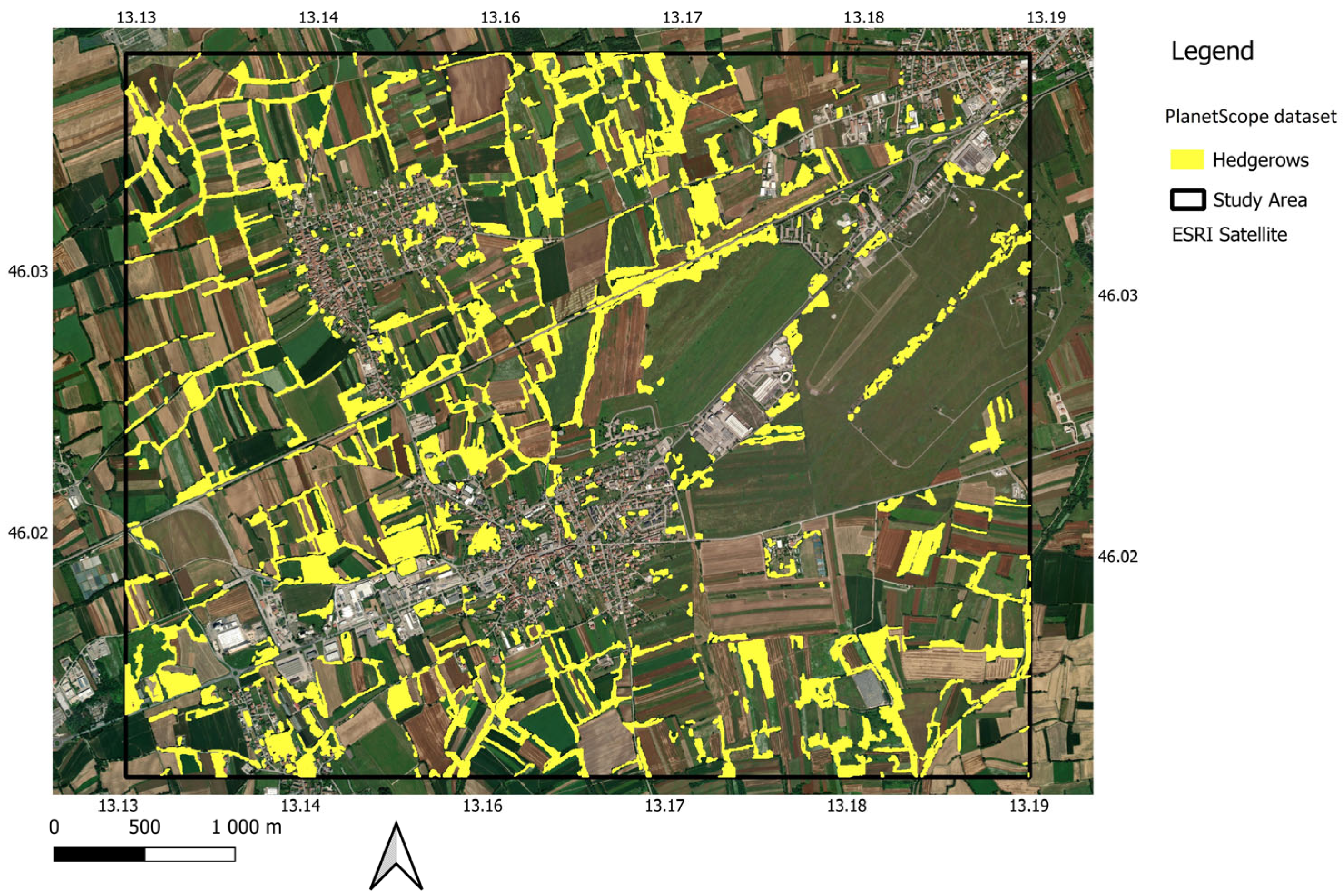
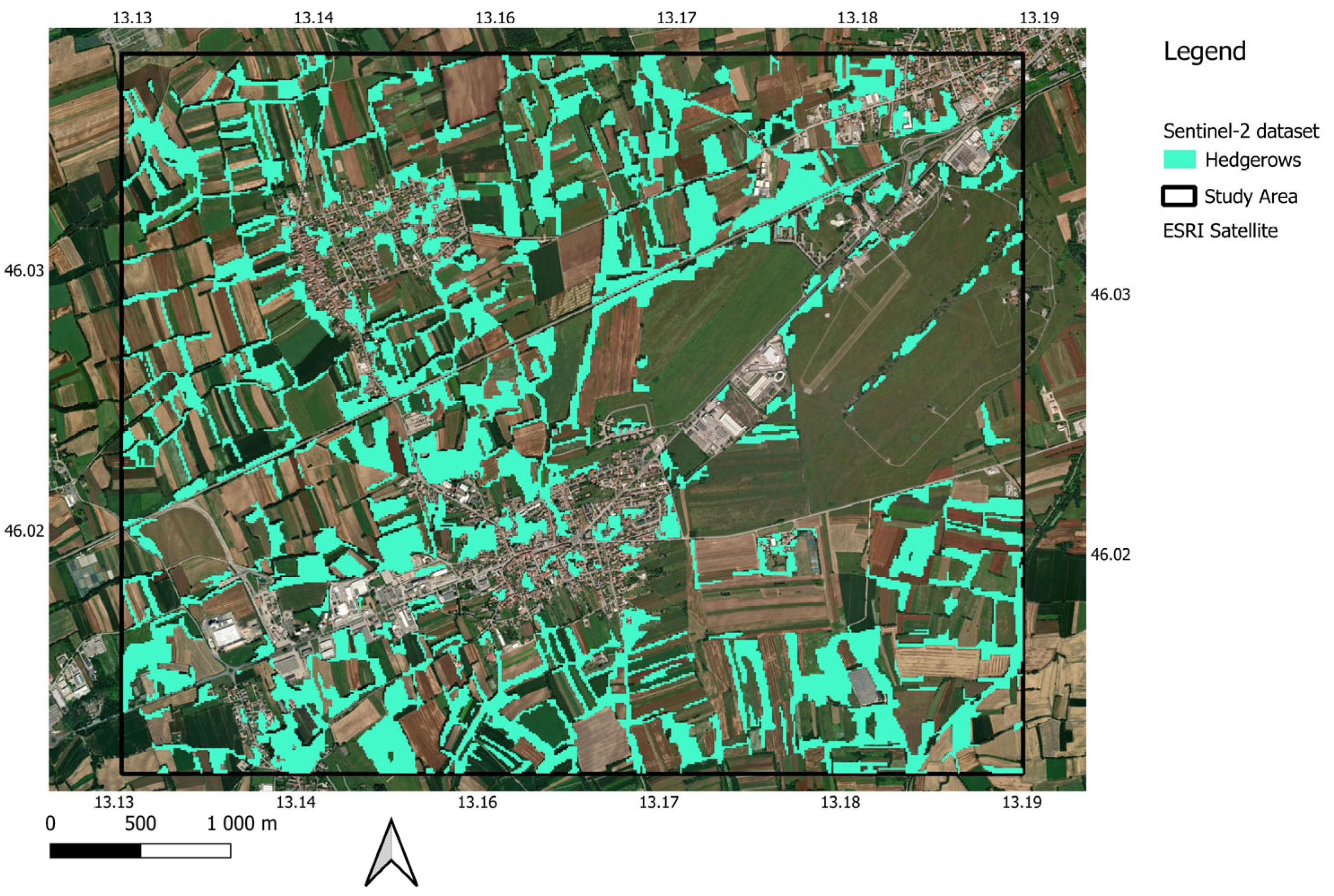
The study area is located in the plain of the Friuli Venezia Giulia region (North-Eastern Italy) in a context of rural–urban landscape, between 46°2′38.05″N latitude, 13°7′45.45″E longitude (Figure 1). The area is characterized by a mixed mosaic of intensively and extensively cultivated areas enriched by tree formations generally dominated by black poplar (Populus nigra L.) or willow thickets of Salix eleagnos Scop. and Salix purpurea L., often contaminated by invasive exotic species (e.g., Robinia pseudacacia L., Amorpha fruticosa L., and Reynoutria japonica Houtt.). The soils of the area consist mainly of Quaternary sand, silt, and silt–clay sediments formed by glacial fluvial transport during the Pleistocene and alluvial deposition during the Holocene.

To address the issue of data availability at high resolutions, our study leveraged data from the PlanetScope platform (Planet Labs, Inc., San Francisco, CA, USA, spatial resolution of 3 m/pxl) to which were coupled images from the Copernicus Sentinel-2 platform (European Space Agency, Paris, France, EU, spatial resolution of 10 m/pxl). The Sentinel-2 bands used include B8 Near-Infrared (NIR) at 842 nm, B2 (Blue) at 490 nm, B3 (Green) at 560 nm, and B4 (Red) at 665 nm. The bands for PlanetScope included B2 (Blue), B4 (Green), B6 (Red), and B8 (Near-Infrared, NIR) at 780–860 nm.

To mitigate the impact of cloud cover on data, a pre-processing step was performed using the Google Earth Engine platform for Sentinel-2 images, applying a cloud filter threshold of 20%. For PlanetScope images, a 10% cloud cover threshold was set within the PlanetScope platform. The difference in cloud cover thresholds was chosen based on the revisit time of each satellite. Sentinel-2 has a longer revisit time compared to PlanetScope’s daily acquisitions.

To increase the possibility of obtaining an image that is temporally aligned with PlanetScope data, we utilized a higher threshold of cloud cover for Sentinel-2. The approach gave us a better temporal match between datasets, yet retaining sufficient image quality for analysis.

Data acquisition encompassed vegetation and non-vegetation seasons, explicitly focusing on April, July, and November 2022 (

Table 1. Multitemporal image data.

		Satellite Data
		Sentinel-2	PlanetScope
Acquisition date	Spring season	28 April 2022	29 April 2022
	Summer season	12 July 2022	13 July 2022
	Autumn season	6 November 2022	13 November 2022

). A total of six images were collected during these months to capture seasonal variability and provide a robust dataset for subsequent analysis.

Very high resolution (VHR) true color orthophotos (Regione Friuli Venezia Giulia) were used for validation. The acquisition period was from 2017 to 2020; the spatial resolution is 20 cm/px.

2.2. Methods

The proposed method used the GEOBIA paradigm, with object-oriented classification of the images performed in eCognition Developer 10.3 software of Trimble Germany GmbH (München, Germany). The applied approach began with a segmentation and classification of the images to distinguish hedgerows from other land cover classes. A second round of segmentation and classification was performed to improve the accuracy and refine the results, focusing on addressing misclassifications and enhancing the detection of hedgerows. Finally, a validation phase was implemented.

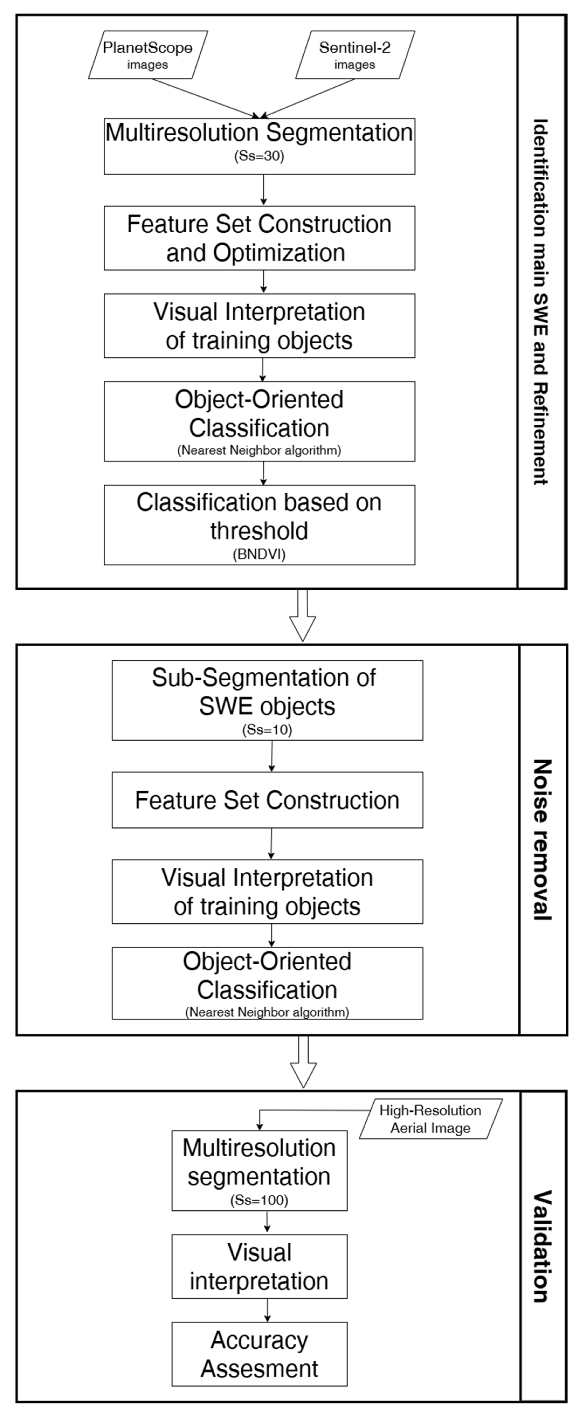
The workflow (Figure 2) consisted of three main steps: (1) identification of the main SWE and refinement, (2) noise removal, and (3) validation.

The workflow includes the initial segmentation, feature set construction, object-oriented classification with the Nearest Neighbor algorithm, and subsequent refinements. Validation was performed using reference data and visual interpretation on orthophotos. QGIS 3.34.10 Prizren (QGIS Development Team. QGIS Geographic Information System, version 3.34. Open Source Geospatial Foundation) was used to handle spatial datasets and perform Geographical Information System (GIS) operations. eCognition 10.3 software was employed for object-based image classification, and finally, Microsoft Excel 2019 was used for deriving statistical analyses.

2.2.1. Image Segmentation

The first phase of the rule set was segmentation, which partitioned the Sentinel-2 and PlanetScope images into distinct and homogeneous regions based on feature properties, such as texture, color, or brightness [42]. A multiresolution segmentation method was adopted [41]. In this region-growing approach, pixels are initially treated as individual objects and then iteratively merged based on similarity to form larger, homogeneous segments [43]. Previous research has consistently identified determining optimal segmentation parameters as a significant challenge [44]. Parameters such as segmentation scale (Ss), shape (Sh), and compactness (Cm) are often determined through trial-and-error methods [45]. In our study, the Ss has been set to 30, ensuring that linear vegetation elements were accurately represented without excessive fragmentation. The shape and compactness parameters were set to 0.8 and 0.2, respectively. This was achieved through an iterative optimization process aimed at finding the best balance between (i) spectral homogeneity and object shape, and (ii) geometric fidelity to the target object and segmentation performance.

The segmentation process relies not only on shape and size (i.e., Ss, Sh, and Cm) criteria, but also incorporates spectral features (

Table 2. The table outlines the image layers used in the segmentation, along with their descriptions and the weights assigned to each layer.

Image Layer	Description	Weights
Red, Green, Blue, Near-Infrared bands	April and July	1
$NDVI$apr, $NDVI$jul	${\displaystyle \frac{(\mathrm{N}\mathrm{I}\mathrm{R}-\mathrm{R}\mathrm{e}\mathrm{d})}{(\mathrm{N}\mathrm{I}\mathrm{R}+\mathrm{R}\mathrm{e}\mathrm{d})}}$	2
$d{NDVI}_{jul-apr}$	${\mathrm{N}\mathrm{D}\mathrm{V}\mathrm{I}}_{\mathrm{j}\mathrm{u}\mathrm{l}}-{\mathrm{N}\mathrm{D}\mathrm{V}\mathrm{I}}_{\mathrm{a}\mathrm{p}\mathrm{r}}$	4

). In this regard, unlike conventional segmentation approaches that depend solely on single-date spectral properties, we introduced multitemporal NDVI differences (Normalized Difference Vegetation Index) as a key segmentation feature to distinguish stable vegetated elements, such as hedgerows, from agricultural areas with seasonal spectral variations [46,47]. This approach is particularly useful in agroecosystems where crops exhibit strong phenological cycles that affect their spectral response over different collection periods [48]. Cropland spectral response at different phenological stages was found to be sensitive to the variations of the growth variables that characterized plant seasonal development [49]. The growing season gives a positive response regarding NDVI values, while the spectral response results in lower NDVI values during the harvest period. In this study, the difference in NDVI between summer and spring is hypothesized to be significant for the different crops, while minimal or no difference in values corresponds to objects exhibiting stable vegetation characteristics, such as hedgerows.

Based on these considerations, we selected as spectral features not only individual multispectral bands (Red, Green, Blue, Near-Infrared), which help distinguish basic spectral differences across land cover types, but also NDVI values from different time periods. Specifically, NDVI for April and July were used to capture vegetation greenness at two distinct times of the year, facilitating the identification of vegetated versus non-vegetated areas. Multitemporal information was then used to compute a new layer representing the difference in NDVI values between July and April.

Each spectral feature was assigned a specific weight based on its relevance in distinguishing target objects (see Table 2). Similarly to Ss parameters, the weight assignment process was not automated but required iterative testing—a widely used method to define weights in OBIA [50,51]—in order to develop a setup that enabled optimal differentiation between hedgerows and other land uses.

2.2.2. Feature Space Construction

Each image object has a variety of characteristics, including spectral, geometric, spatial, topological, and hierarchical attributes. These measurable properties of an image object, such as its color, texture, or compactness, are utilized in the classification process and are called features. An object can be assigned to a particular class depending on the feature value. A multitemporal detection of changes helps to differentiate objects exhibiting high NDVI variability from those maintaining a more constant value, thereby enhancing classification accuracy. So, multitemporal profiles of the NDVI layer were identified as attributes useful for the classification.

In order to classify the objects, a set of features were extracted. Various categories of features are commonly employed for the classification of agricultural regions, including spectral, textural, structural, and geometric attributes [52]. Here, we used a combination of spectral and textural features (

Table 3. Set of features extracted for the classification process.

Object Features	Description
$d{NDVI}_{jul-apr}$	${NDVI}_{jul}-{NDVI}_{apr}$
$d{NDVI}_{jul-nov}$	${NDVI}_{jul}-{NDVI}_{nov}$
Maximum difference
Brightness
GLDV Entropy (quick 9/11) (90°)	$-{\displaystyle \sum _{i,j}}{p}_{ij}\log \left(p_{ij}\right) where p_{ij}={\displaystyle \frac{x_{ij}}{\sum _{i,j}{x}_{ij}}}$

) for discriminant hedgerows and other land covers.

To optimize the set of features for classification, we adopted a two-step selection process. First, the existing literature was reviewed to identify features used in similar studies. Based on this, we initially considered a range of 11 spectral and textural features [46,47,48,53]. Second, we used the Feature Space Optimization tool (FSO) in eCognition, which allowed us to refine the selection and use only the most influential features. FSO is a tool available in eCognition and it calculates an optimum feature combination based on class samples. FSO evaluates the Euclidean distance in feature space between the samples of all classes and selects a feature combination resulting in the best class separation distance, which is defined as the largest of the minimum distances between the least separable classes [54].

This method evaluates class separability based on different features and helps to identify those that maximize classification accuracy, and is commonly used in studies using eCognition (e.g., [50,55]).

The five most influential features extracted with FSO were Brightness, GLDV Entropy (quick 9/11) (90°), Maximum difference, and differences in NDVI mean values between July and April and between July and November (the full list of features and the results of FSO process are available in Supplementary Materials). These features were chosen for classification because substantial differences in the spectral response of agricultural fields can be identified between the different seasons. The other spectral features considered included Maximum difference, which informs on the spectral variability within an object, and Brightness and Entropy, which measure the spectral heterogeneity. Entropy was derived from the Haralick texture features, a set of statistical measures used to describe an image’s texture. These features were introduced in the 1970s and are widely used in image analysis and computer vision to characterize the spatial arrangement of image pixel intensities [53,56,57]. The Haralick texture features are derived from the grey-level co-occurrence matrix (GLCM) and grey-level difference vector (GLDV), quantifying distance and angular spatial relationships within specific image sub-regions [58]. GLCM and GLDV texture measures provide information about the spectral differences between neighboring pixels. From the GLDV texture features, we selected the GLDV Entropy (quick 9/11) (90°). GLDV Entropy (quick 9/11) (90°) in eCognition calculates the entropy of the gradient direction distribution using a 9 × 11 quick neighborhood with a vertical (90°) gradient direction.

2.2.3. Classification and Refinement

The Nearest Neighbor (NN) classification approach was adopted to categorize hedgerows. This technique assigns membership values to image objects by comparing them to a set of reference samples from known classes. The classification process involves two main steps:

• Training phase when the system learns from representative sample objects;
• Classification phase is where image objects are assigned to the class of the nearest sample in feature space. Proximity is determined by calculating the distance between the image objects and each sample, with distance values standardized using the standard deviation of all feature values. This approach allows for a flexible and efficient categorization of image objects, relying on their nearest representative samples [54].

To classify the created objects into the classes “Hedgerows” and “Other”, the Nearest Neighbor classifier was trained with samples manually labeled in eCognition. The number of training samples for each class within the study area was 60. The training samples represent 60 polygons resulting from the segmentation. Each of those cells contains values of at least 100 pixels for that class. These samples were chosen randomly; the same procedures were followed for validation.

A second classification step was performed by assigning class labels to the image objects based on a threshold value. This step utilized the Blue Normalized Difference Vegetation Index (BNDVI) as the sole feature. Unlike NDVI, which relies on the Red and Near-Infrared (NIR) bands, BNDVI utilizes the Blue and NIR bands, making it more susceptible to atmospheric interference and variations in ground moisture. Several studies have reported that the BNDVI can effectively contribute to the spatial variability and distribution of chlorophyll within ecosystem assessment [59,60]. Gallegos et al. (2023) investigated tree health evaluation in urban green areas using different findings and significant correlations between BNDVI and variables such as crown density and transparency [61]. Furthermore, the use of BNDVI has demonstrated strong spatial and environmental coherence in previous studies [62], so BNDVI offers a complementary approach that can potentially enhance the accuracy and interpretability of classification results.

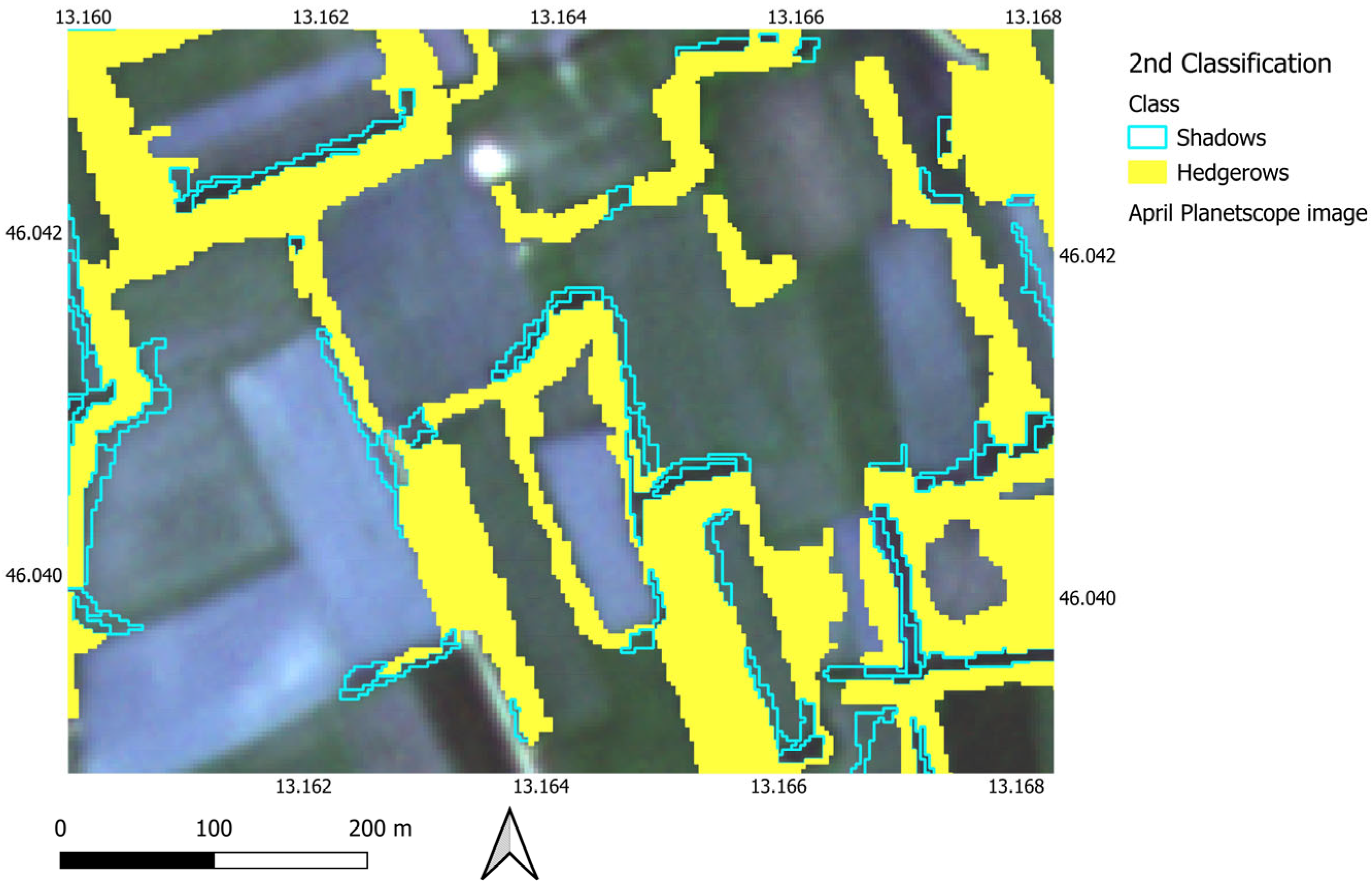
2.2.4. Noise Removal

Shadows are a common artefact in high-resolution remote sensing imagery arising from variations in terrain illumination captured by satellite sensors. Shadows can significantly hinder imagery analysis diminishing spectral radiance in shaded areas, making it challenging to separate spectral and spatial features within them [63,64]. Moreover, shadows are often misclassified as water or water-related land cover due to spectral and texture similarities with water bodies [65]. Given their detrimental impact on object classification, accurate shadow detection and removal are crucial for effective image analysis. In our case, shadows represent a false hedgerow encumbrance, distorting the size and shape of the target object. To detect shaded areas misclassified as hedgerows, shadows were explicitly addressed by identifying them as a distinct class. As shaded areas often appear contiguous with vegetation, they were identified through a refined sub-segmentation process applied exclusively to the “Hedgerow” class. To this aim, a scale parameter of 10, a shape factor of 0.8, and a compactness factor of 0.2 were used. The image layer weights employed in this sub-segmentation were consistent with those used in the previous segmentation step. The feature space for this sub-segmentation was defined considering the spectral absorption characteristics in the infrared and red spectral ranges. Four distinct features were defined to characterize this space, as reported in

Table 4. Spectral features selected to enhance the distinction between hedgerows and adjacent shadows.

Feature Space Elements	Description
Brightness
NDVIjul	${\displaystyle \frac{(NIR-Red)}{(NIR+Red)}}$
∆R − G	Red-Green
R/IR	Red/NIR

.

The Brightness feature was considered crucial because shaded areas exhibit brightness imbalance characterized by low reflectivity and the appearance of dark pixels, which can significantly interfere with analysis [66]. Recent shadow detection methods effectively leverage the NIR band to improve the segmentation of shadowed regions in imagery [28]. While shadows diminish reflectance across all spectral bands, this effect is more pronounced in the NIR band compared to the Red. The Red/NIR ratio effectively highlights these differences, increasing the contrast between illuminated and shadowed areas. This consideration is crucial given that completely dark objects often exhibit higher reflectivity values in the Near-Infrared spectrum [64,67].

A second supervised classification employing the same Nearest Neighbor algorithm as in the previous step was implemented within the eCognition environment to differentiate shadows from the initially classified hedgerows. The classification scheme included two classes: “Hedgerows” and “Shadows”. A total of 30 training samples were collected for each class within the study area.

2.2.5. Validation

To ensure robust validation, we adopted a two-step approach combining automated segmentation and visual interpretation. A validation dataset was derived from high-resolution orthophoto maps segmented in eCognition, producing structured reference polygons.

The orthophotos, provided by Friuli-Venezia Giulia Region—Central Directorate for Property, State Property, General Services, and Information Systems—are characterized by 0.20 m resolution and include RGB and Near-Infrared bands. This high spatial resolution provided a more robust validation dataset for comparison and helped to mitigate potential segmentation errors.

The orthophoto was segmented in eCognition using a scale parameter of 100, a shape factor of 0.8, and a compactness factor of 0.2. Unlike the segmentations performed during the hedgerow detection phase, this analysis utilized a mono-temporal layer. The NDVI was calculated, and image layer weights were assigned as follows: 4 for the NDVI and 2 for the NIR.

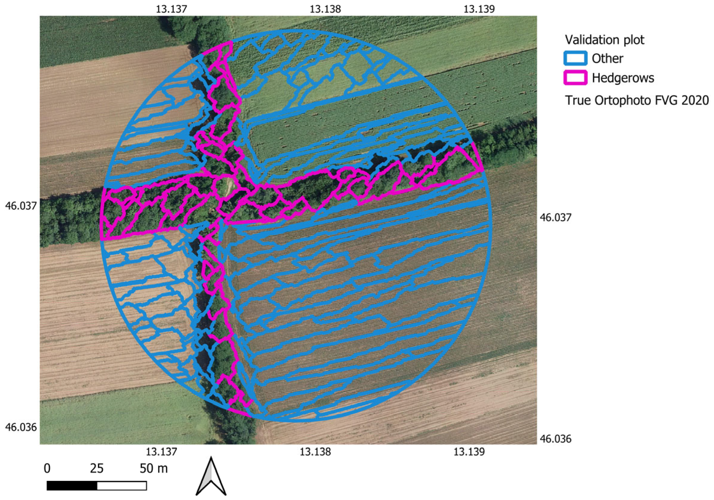
To ensure classification reliability, an independent polygon classification was conducted across a substantial portion of the study area. Sampling units consisted of circular plots of 3 ha [50], with centers randomly selected using a systematic unaligned sampling design across a grid with 1 km² with square cells (4 × 5 km). Each square cell contained a circular plot intersecting one or more “Hedgerows” or “Other” image polygons. All polygons within each circular plot were visually interpreted (Figure 3) and assigned to one of two classes: 0 for “Other” and 1 for “Hedgerows”. This served as “ground truth” data for map validation. The validation dataset encompassed 3.0% of the study area, and 4595 polygons were visually interpreted (

Table 5. Classification of polygons for map validation.

Class	Number of Polygons	Surface (ha)	%
Hedgerows	881	8.21	14
Other	3714	52.01	86
Total	4595	60	100

).

By using automated segmentation, we ensured standardized object boundaries, while visual interpretation refined classification reliability.

The first step, i.e., automatic segmentation of orthophotos in eCognition, provided a structured dataset of objectively delineated polygons, avoiding the subjective biases that can arise from manual delineation.

Compared to full visual interpretation, this approach provides a better spatial distribution of validation samples across the study area, while significantly reducing the time required to generate the dataset. Segmentation-based validation also improves comparability with object-based classification results, ensuring consistency in data processing. This two-step approach effectively balances accuracy, spatial representativeness, and time efficiency, thereby increasing the robustness of the validation dataset.

A confusion matrix was built to evaluate classification accuracy by comparing the object-based classified image with polygons of visually interpreted data. Validation and training samples did not overlap. The kappa coefficient was also calculated to assess the agreement between the two classifications. Overall accuracy, producer’s accuracy, and user’s accuracy were calculated, offering a comprehensive assessment of method performance and reliability in mapping hedgerows within the study area.

The confusion matrix is a two-dimensional table that compares the actual classes of objects to their predicted classes, including information about accurate and predicted classifications made by a classification system [68].

By converting sample counts into estimated areas, we evaluated overall accuracy (OA), producer’s accuracy (PA), and user’s accuracy (UA), providing a robust accuracy assessment of our classification results concerning both Sentinel-2 and PlanetScope data.

3. Results

3.1. Image Segmentation and Classification

The first level segmentation of the PlanetScope dataset yielded 11,844 objects, while the Sentinel-2 dataset produced 1582 objects. The mean area of segments was approximately 1700 m² for PlanetScope and 12,600 m² for Sentinel-2, reflecting the higher spatial resolution of PlanetScope imagery (

Table 6. Statistics of the initial segmentation of the PlanetScope and Sentinel-2 datasets.

Statistics 1st Segmentation
Dataset	Count	Min Value [m2]	Max Value [m2]	Mean [m2]	Median [m2]
PlanetScope	11,844	54,016.0	27,116.2	1691.4	1269.4
Sentinel-2	1582	100.0	149,747.2	12,589.2	9903.0

).

The objects classified as “Hedgerows” were subsequently sub-segmented into smaller objects to identify and separate adjacent shadow areas, potentially false positives. These shaded regions were often misclassified as hedgerows. The initial class “Hedgerows” for the PlanetScope dataset included 2157 objects. The sub-segmentation process resulted in a total of 10,345 objects. For the Sentinel-2 dataset, the initial “Hedgerows” class comprised 437 objects (Figure 4).

After the second classification, the shaded regions were eliminated and moved to the “Other” class. Analysis of the map derived from classification of PlanetScope images revealed that shadows covered approximately 3.6% of the mapped area, whereas Sentinel-2 imagery indicated shadow coverage of approximately 7.9% of the total surface.

The detailed statistics of shadow coverage and classification accuracy are reported in

Table 7. Surface area statistics of different features after the second segmentation and classification for both datasets.

PlanetScope Dataset
			[m2]
Class_Name	Count	Min	Max	Mean	Median
hedgerow	7366	27.0	2133.7	307.8	270.1
shadow	2967	27.0	1395.4	242.3	207.1
subseg_unclassified	12	18.0	486.2	207.8	139.5
total	10,345	-	-	-	-
Sentinel-2 Dataset
			[m2]
Class_Name	Count	Min	Max	Mean	Median
Hedgerow	960	100.0	13.604.3	1630.5	1300.4
Shadow	2198	100.0	12,203.8	1878.6	1600.5
subseg_unclassified	9	100.0	1300.4	333.4	200.1
Total	3167	-	-	-	-

, while Figure 5 and Figure 6 illustrate the final mapping results after the second classification.

Analysis of the higher resolution PlanetScope dataset identified 226 hectares of hedgerows, which constitute 11.3% of the study area. Conversely, in the Sentinel-2 dataset, the analysis revealed 292 hedgerows (413 hectares), accounting for 2.7% of the study area (

Table 8. Area and number of elements for each class after classification for both the PlanetScope and Sentinel-2 datasets.

	Classes	Area [ha]	% Area	n° Elements
PlanetScope dataset	Hedgerow	226	11.3	533
	Other	1774	88.7
Sentinel-2 dataset	Hedgerow	413	20.7	292
	Other	1587	79.3

).

3.2. Accuracy Assessment

Accuracy assessment is crucial in remote sensing-based mapping to evaluate the reliability of the resulting maps. In this context, the producer’s and the user’s accuracy are key metrics used to quantify the classification algorithm’s performance by applying a confusion matrix to each dataset.

Table 9. Confusion Matrix for the PlanetScope and Sentinel-2 datasets.

PlanetScope Data		Actual [ha]
		Other	Hedgerow
Predicted [ha]	Other	50.59	1.75
	Hedgerow	1.42	6.46
Sentinel-2 Data
		Other	Hedgerow
Predicted [ha]	Other	45.07	2.41
	Hedgerow	6.92	5.80

shows the actual and predicted areas (in hectares) for each class (Other and Hedgerow).

The assessment (

Table 10. Accuracy metrics for both the PlanetScope and Sentinel-2 data.

PlanetScope Dataset		Other	Hedgerow
User’s Accuracy	-	0.97	0.82
Producer’s Accuracy	-	0.97	0.79
Overall Accuracy	0.95	-	-
K Cohen	0.77	.	-
Sentinel-2 Dataset		Other	Hedgerow
User’s Accuracy	-	0.95	0.46
Producer’s Accuracy	-	0.87	0.71
Overall Accuracy	0.85	-	-
K Cohen	0.47	-	-

) reveals an overall accuracy of 95% for PlanetScope data, demonstrating a good performance. Specifically, the producer’s accuracy for the “Hedgerows” class is 0.79, indicating that 79% of the reference area identified as hedgerows on the ground are correctly classified as such in the map derived from PlanetScope images. The user’s accuracy of 0.82 suggests that 82% of the area classified as hedges in the map correspond to actual hedges on the ground.

For Sentinel-2 data, the confusion matrix shows an overall accuracy of 85%. While the producer’s accuracy for the “Hedgerows” class is 71%, the user’s accuracy is 46%, suggesting lower reliability in correctly identifying and classifying hedgerows than the PlanetScope dataset.

Cohen’s Kappa coefficient (K) further highlights the differences between the two datasets. A K value of 0.77 for PlanetScope data indicates substantial agreement between classification and reference data, while the Sentinel-2 dataset, with a K of 0.47, shows only moderate agreement, reflecting higher classification uncertainty.

3.3. Comparison with SWF Copernicus Dataset

A comparison with large-scale datasets, such as the Copernicus Small Woody Features (SWF) (https://land.copernicus.eu/en/products/high-resolution-layer-small-woody-features, accessed on 10 April 2024), revealed a significant underestimation of hedgerow presence within the study area. The Copernicus SWF dataset estimated hedgerow coverage at just 6.2% of the total area. In contrast, our method using Sentinel-2 data estimated hedgerow coverage at 20.7%, showing a substantial discrepancy in area coverage. This marked difference highlights the limitations of the Copernicus SWF dataset in accurately capturing hedgerow coverage at a local scale. The SWF dataset, generated at a pan-European scale, may not account for the finer spatial variability of hedgerows, leading to a more generalized and lower estimate.

Further refining our approach, we applied PlanetScope data, which detected hedgerow coverage at 11.3% (Figure 7). This estimate lies between the two previous ones—significantly higher than the Copernicus SWF estimate but lower than the Sentinel-2 estimate—providing a more nuanced and precise depiction of hedgerow coverage.

A spatial comparison between the two datasets was conducted. After excluding the SWF polygons not detected with Sentinel-2 imagery and removing polygons mapped with Sentinel-2 imagery that contained no SWF features, we observed that each hedgerow polygon derived from Sentinel-2 data contains an average of three SWF elements. This suggests that the SWF dataset represents hedgerows as fragmented entities.

Similarly, for hedgerows mapped using PlanetScope data, each extracted hedgerow corresponds to an average of 1.96 SWF elements. The lower ratio compared to Sentinel-2 shows PlanetScope’s greater ability to represent hedgerows as continuous features while still accounting for the presence of gaps. The lack of continuity detected in SWF is possibly due to differences in mapping methodology, resolution, or classification method.

4. Discussion

This study aimed to develop a semi-automatic method for extracting hedgerows using multitemporal and multispectral satellite imagery. A key focus was comparing datasets with varying spatial resolutions to assess the effectiveness of the object-oriented approach (OBIA).

A significant challenge in hedgerow monitoring is the lack of up-to-date local inventories. While programs like Copernicus provide broad overviews, large-scale datasets often lack the necessary temporal resolution and detail for precise site-specific monitoring. This is particularly crucial as hedgerow structures and configurations change rapidly at the local scale, requiring frequent data updates to map this dynamic feature accurately [69]. The lack of localized, semi-automatic tools that can efficiently track hedgerows’ presence and topological accuracy further complicates conservation and management efforts.

By implementing OBIA, we sought to improve the delineation and characterization of small and linear vegetation elements, like hedgerows, overcoming the limitations of traditional pixel-based analysis. Our goal was to enhance the extraction accuracy of these ecologically essential features, thereby contributing to more precise mapping and better management of landscape elements in agroecosystems [70].

The results provide valuable insights into the potential of multiresolution and multitemporal data for refining detection and classification of hedgerows. Furthermore, by comparing results from imagery with different spatial resolutions (3 m from PlanetScope and 10 m from Sentinel-2), we could evaluate the effectiveness of the object-oriented approach in delineating hedgerows.

Utilizing a multitemporal dataset proved highly beneficial, enabling the detection of seasonal vegetation changes and effectively differentiating between agricultural fields and stable linear vegetation elements. This study demonstrated robust classification results achieved by constructing a suitable feature space and employing the Nearest Neighbor classifier, further refined through shadow removal techniques.

The results showed that higher spatial resolution data (PlanetScope) significantly improved hedgerow extraction accuracy, as confirmed by the accuracy assessment. Integrating multitemporal NDVI differences and Haralick texture features, our methodological approach effectively distinguished hedgerows from other land cover types. The PlanetScope dataset achieved an overall accuracy of 95%. Such a result is comparable to accuracies achieved in other studies [71], but even higher than that of recent studies using very-high-resolution satellites (IKONOS) [72].

The accuracy assessment of the Sentinel-2 data indicated a good overall accuracy (85%), but exhibited a low user accuracy (47%), suggesting an overestimation of the hedgerow presence. The overestimation is attributable to the lower spatial resolution (3 times lower than PlanetScope), which increases the influence of mixed pixels in defining the target class. This issue was evident during the segmentation phase, as hedgerows are often smaller than the 10 × 10 m pixel unit, leading to errors in polygon generation. The commission error, representing the percentage of areas incorrectly classified as “Hedgerows”, is notably high at 54%. This overestimation is further evidenced by the significantly larger area mapped (nearly double) as hedgerows using Sentinel-2 data compared with PlanetScope data.

While both datasets exhibited good overall accuracy, slightly higher measures of accuracy can be found in the literature. It should be noted that these studies often rely on presence/absence validations using control points [34,73]. In contrast, our validation aimed to assess the accuracy of the presence/absence predictions and the actual mapped area. We employed an independent dataset (regional orthophoto) to extract the surface area of the target element. Subsequently, an area comparison was conducted to verify the topological correctness of the elements mapped by our model. The results demonstrated good user accuracy and producer accuracy, especially for PlanetScope data, with values of 0.87 and 0.71, respectively.

The results of the comparison of the maps produced in our study and SWF dataset suggest that PlanetScope imagery offers a balanced compromise, capturing more detailed local features than Sentinel-2 while reflecting a broader view than the Copernicus SWF dataset. Our results are in line with previous studies that have highlighted limitations of the SWF dataset in capturing linear vegetation structures. For example, Huber Garcia et al. (2025) [74] mapped hedgerows in Bavaria using high-resolution orthophotos and convolutional neural networks, finding that approximately 43% of the identified hedgerows were absent from the SWF layer. This suggests that the SWF dataset may struggle to detect narrow and elongated vegetation elements, reinforcing the need for high-resolution mapping approaches. Similarly, Ahlswede et al. (2021) [72] demonstrated that convolutional neural networks applied to very-high-resolution IKONOS imagery outperformed traditional classification methods in hedgerow detection. These findings emphasize that while large-scale datasets such as Copernicus SWF provide a valuable baseline, accurate hedgerow mapping often necessitates the use of locally adapted methodologies with higher spatial resolution and advanced classification techniques.

Our findings confirm the importance of selecting the appropriate spatial resolution for accurate mapping at the local scale. While European-scale maps provide valuable baseline information, achieving accurate hedgerow area and boundary estimates often necessitates applying locally scaled methods.

The current availability of free satellite data does not yet match the spatial resolution provided by commercial platforms such as PlanetScope. However, future technological advancements may lead to higher-resolution imagery becoming accessible on non-commercial platforms as well. At present, the proposed method with the PlanetScope dataset is not directly scalable at a continental level. However, with a moderate investment, its applicability on a regional scale is feasible. It is also worth noting that PlanetScope imagery is offered under a variety of subscription plans for research and institutional use, and PlanetScope also provides non-commercial access through programs such as the Copernicus Data Space Ecosystem and the Norwegian International Climate and Forest Initiative tropical forest monitoring program. In addition, environmental agencies and public institutions can access high-resolution imagery under special agreements at reduced rates or through special partnerships. Compared to commercial VHR imagery, PlanetScope’s daily revisit time and 3 m spatial resolution make it a cost-effective alternative for land-monitoring applications that require frequent updates.

This study demonstrates that, in the future, the approach could potentially be extended to larger spatial scales. The method is likely transferable to other contexts with a predominantly agricultural landscape where hedgerows are a minor landscape element, as the selected features are characteristic of hedgerows and should remain relevant across similar environments. However, a potential limitation may arise in regions where hedgerows are narrower than those in Friuli-Venezia Giulia. In such cases, the source of the dataset and the spatial resolution would have to be re-evaluated to ensure accurate detection and classification. On the other hand, in regions with very large hedges, it may be sufficient to use data already completely free, such as Sentinel-2.

In terms of software implementation, eCognition was chosen because of its robust Object-Based Image Analysis (OBIA) capabilities, which can perform segmentation and classification of SWEs based on spectral and spatial features. eCognition has a flexible rule-based classification and machine learning environment that is suitable for working with high-resolution imagery.

Other potential limitations of the study include challenges with both Sentinel-2 data resolution and the processing of high-resolution imagery in eCognition. Extracting numerous features for target identification required substantial processing time, hindering the method scalability, especially for larger areas. The increased data volume of larger study areas exponentially extends computation time, potentially making analysis prohibitive. Furthermore, processing a high number of features complicates and reduces the efficiency of the analysis. Secondly, our method was developed based on the specific landscape characteristics of the study area. Therefore, careful consideration must be given to potential variations when applying this methodology to other contexts.

Our approach shows promise for mapping hedgerows, but several technical challenges remain. Future work could involve incorporating a broader range of spectral indices and exploring more advanced processing algorithms to enhance classification accuracy, especially in differentiating hedgerows from adjacent vegetation types.

In addition, integrating additional data from remote sensing technologies like elevation data from Light Detection and Ranging (LiDAR) would provide crucial information for defining landscape structure [75], especially combining aerial and terrestrial laser scanning [76]. This combination would allow a more comprehensive characterization of the three-dimensional structure of vegetation elements. However, it is worthy to note that aerial LiDAR is not available everywhere and usually, LiDAR scanning has a low revisiting time. Indeed, increasing the temporal frequency of data collection would provide more detailed information about seasonal dynamics and lead to more robust hedgerow detection.

5. Conclusions

Our research develops a semi-automatic method for SWE extraction using Object-Based Image Analysis on high-resolution satellite imagery, comparing the performance of our method on PlanetScope and Sentinel-2 data. By integrating multitemporal spectral indices and texture-based features, we have improved object mapping and classification accuracy. Furthermore, our approach has addressed the limitations of existing datasets, such as the Copernicus SWF inventory, by constructing a more frequently updated and adaptable mapping solution. Finally, we have analyzed the critical aspects of our method and discussed additional data sources that could be integrated to further improve the SWE mapping.

The results indicate that PlanetScope data achieved significantly higher accuracy, whereas Sentinel-2 data, despite their coarser resolution, confirmed an overall accuracy (OA) exceeding 80%. This comparative analysis illustrates the potential of using open-source and high-resolution commercial imagery for hedgerow detection. Secondly, the classification method applied in this study enhances the feasibility of developing a comprehensive database and addresses the challenge posed by the absence of a standardized reference dataset. Such a dataset would improve research comparability, foster collaboration, and drive progress, ensuring future applications. Moreover, these findings will contribute to advancing hedgerow detection research and deepening the understanding of hedgerows’ ecological significance, thereby supporting sustainable land management and biodiversity conservation.