A Fusion Method Based on Physical Modes and Satellite Remote Sensing for 3D Ocean State Reconstruction

Abstract

Accurately and timely estimating three-dimensional ocean states is crucial for improving operational ocean forecasting capabilities. Although satellite observations provide valuable evolutionary information, they are confined to surface-level variables. While in situ observations can offer subsurface information, their spatiotemporal distribution is highly uneven, making it difficult to obtain complete three-dimensional ocean structures. This study developed an operational-oriented lightweight framework for three-dimensional ocean state reconstruction by integrating multi-source observations through a computationally efficient multivariate empirical orthogonal function (MEOF) method. The MEOF method can extract physically consistent multivariate ocean evolution modes from high-resolution reanalysis data. We utilized these modes to further integrate satellite remote sensing and buoy observation data, thereby establishing physical connections between the sea surface and subsurface. The framework was tested in the South China Sea, with optimal data integration schemes determined for different reconstruction variables. The experimental results demonstrate that the sea surface height (SSH) and sea surface temperature (SST) are the key factors determining the subsurface temperature reconstruction, while the sea surface salinity (SSS) plays a primary role in enhancing salinity estimation. Meanwhile, current fields are most effectively reconstructed using SSH alone. The evaluations show that the reconstruction results exhibited high consistency with independent Argo observations, outperforming traditional baseline methods and effectively capturing the vertical structure of ocean eddies. Additionally, the framework can easily integrate sparse in situ observations to further improve the reconstruction performance. The high computational efficiency and reasonable reconstruction results confirm the feasibility and reliability of this framework for operational applications.

1. Introduction

A comprehensive understanding of the nature of the ocean and the ability to predict the movement of seawater are of paramount importance for both oceanographic research and military applications. The most significant physical elements in this regard are temperature (T), salinity (S), and currents (u and v). In the context of ocean forecasting, the accuracy of the initial three-dimensional state of the ocean is pivotal in enhancing the efficacy of forecasting models. The acquisition of oceanic data can be facilitated by diverse methodologies, including in situ observation, satellite surveillance, and numerical simulation. Satellite remote sensing data provide real-time observations of sea surface conditions and have been extensively utilized to analyze various ocean phenomena [1,2,3,4] or forecast surface elements [5,6,7]. Nevertheless, the categories of sea surface elements available from satellite data are relatively limited, with a primary focus on the sea surface temperature (SST), sea surface salinity (SSS), and sea surface height (SSH). This remains inadequate for operational applications, particularly in the context of forecasting underwater ocean state fields, such as T, S, u, and v. In recent years, the establishment of a global network of floats has facilitated the measurement of temperature and salinity at various depths. For instance, the Argo observation system is capable of measuring these variables from the surface down to 2000 m. However, the observed data points are random and discrete. While this information provides valuable insights into temperature and salinity, it is still inadequate for constructing a spatial–temporal continuous field, which is essential for accurate forecasts.

Numerical models simulate the behavior of the ocean’s physical processes based on mathematical equations that represent the ocean’s dynamics [8,9]. These models have the capacity to forecast the future state of the ocean under various scenarios. However, the models are subject to inherent uncertainties arising from assumptions, simplifications in the equations, errors in input data, and limitations of computational power. Considering their inherent uncertainties, data assimilation methods have been developed to integrate numerical ocean models with observational data, thereby producing ocean reanalysis products. These products yield consistent and quality-controlled records, including SSH, T, S, u, and v, among others, from the surface to the depths. Reanalysis products are extensively utilized in studies of ocean dynamics [10,11,12] and for ocean forecasting [13,14]. However, it is crucial to acknowledge that these products are intended to provide valuable historical context and are not suitable for real-time updates.

As subsurface information is of crucial importance for ocean forecasting and assimilation, researchers have attempted to construct three-dimensional ocean fusion products using available data and a variety of methods, mainly including regression analysis and mode extraction techniques. Regression analysis establishes a direct relationship between sea surface variables and subsurface profiles and can provide a continuous description of the three-dimensional state of the ocean. Among the various methods employed, the Modular Ocean Data Assimilation System (MODAS) has demonstrated particular success in the realm of ocean operationalization applications [15,16,17]. The system utilizes multivariate linear regression to reconstruct the three-dimensional thermohaline structure, projecting sea surface height and sea surface temperature information to the subsurface layer [18]. It is noteworthy that the combination of linear regression with optimal interpolation techniques has been successfully employed in the construction of ARMOR3D objective analysis products [19,20]. While regression analysis is capable of utilizing satellite and in situ observations to establish an intrinsic relationship between the three-dimensional state of the ocean, it is challenging to obtain physically reliable temperature and salinity estimates in regions where subsurface observations are lacking. To enhance the physical consistency of the inversion results, the modal extraction method is employed to estimate the three-dimensional thermohaline structure of the ocean. Modal extraction methods are utilized to capture vertical physical correlations by combining the vertical projection patterns of the sea surface and subsurface layers. Examples of such methods include coupled mode methods [21], univariate empirical orthogonal function (EOF) analysis [22,23], and multivariate empirical orthogonal function (MEOF) analysis [24]. Despite the efficacy of this method in capturing interactions between variables, its extension to regions lacking subsurface observations remains challenging [25,26] (e.g., the South China Sea [27]). Furthermore, given that the method establishes modal relationships solely in the vertical direction, its evolutionary information in the horizontal space is frequently disregarded.

In recent years, deep learning (DL) methods, including convolutional neural networks (CNNs) [28,29] and long short-term memory (LSTM) algorithms [30], etc., have demonstrated remarkable efficacy in the estimation of the three-dimensional ocean state. Nevertheless, the majority of extant studies, in order to obtain results that match in situ observations, typically adopt a modeling scheme similar to traditional methods, using in situ observations as labels during model training. This training strategy is heavily reliant on the density of in situ observations, and it thus predominantly focuses on the global area [31] or the open ocean [32]. It is important to note that the uneven spatial and temporal distribution of in situ observations can also lead to poor temporal resolution (mostly monthly averaging) of this type of method. Furthermore, some studies have utilized reanalysis data as a label for training, in conjunction with satellite observations, for the inversion of the underwater thermohaline structure [33]. However, the employment of nonlinear models (e.g., CNNs) of high complexity is frequently observed in the construction of thermohaline relationships in continuous space. Consequently, the DL method incurs a substantial computational cost, which hinders its widespread adoption in operational applications. Meanwhile, it is difficult to incorporate irregularly distributed in situ observations in DL models. Therefore, enhancing the flexibility of existing methods for fusing in situ observations, capturing spatial multi-scale dependencies, and meeting the timeliness requirements for operational applications poses a significant challenge. In order to address the aforementioned issues, the present study focuses on constructing a lightweight model that combines satellite sea surface data with reanalysis data using a simple MEOF method to obtain daily three-dimensional multivariate fields. The extraction of multivariate evolutionary information with physical consistency from the reanalysis data is achieved by utilizing the cross-variate relationships characterized by different modes, thereby enhancing the correlation between satellite observations and subsurface evolution. While ensuring a low computational cost, we can flexibly incorporate available Argo profile observations to improve the reconstruction accuracy, thus meeting the demand for real-time and reliable three-dimensional temperature, salinity, and current fields in operational applications.

In summary, the contributions of this paper are as follows:

(1)

An enhanced lightweight MEOF framework was developed, integrating multivariate data (satellite sea surface observations, historical reanalysis products, and Argo profile observations) in the sparsely observed in situ South China Sea region to achieve high-temporal-resolution (daily) three-dimensional multivariate fields (containing temperature, salinity, and current).

(2)

On the basis of ensuring high computational efficiency, our framework obtained better reconstruction accuracy than the traditional baseline method (MODAS), which can be further generalized to the application of operational ocean forecasting.

The datasets used in this study, along with the methods and experiments involved in the proposed state field reconstruction scheme, are introduced in Section 2. Section 3 presents the results. Section 4 presents the discussion, while Section 5 concludes the paper.

2. Materials and Methods

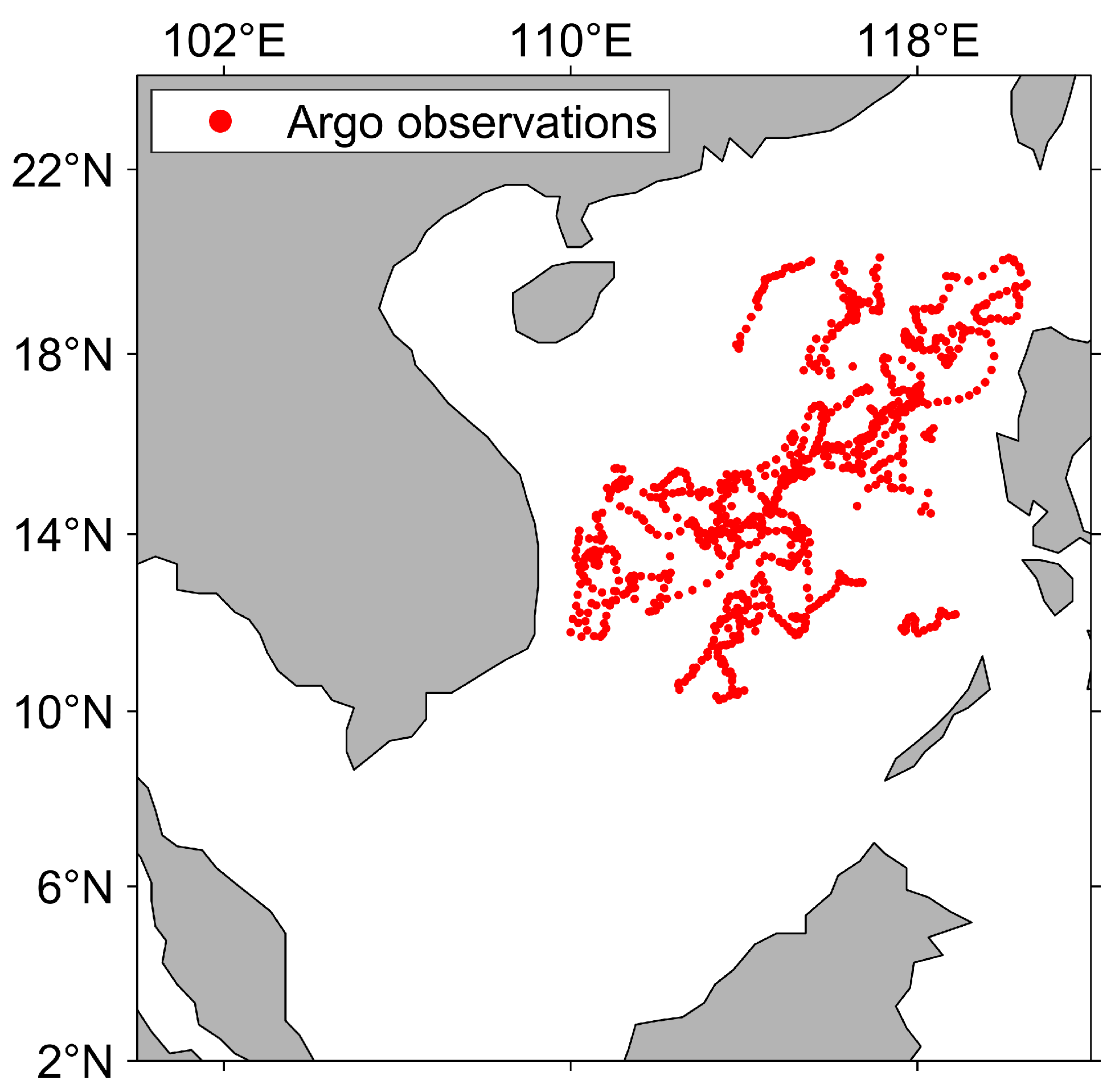
2.1. Study Area

The study area for this research was the South China Sea (SCS), chosen for its complex multi-scale dynamic processes. The geographical scope, as depicted in Figure 1, spans from 2°N to 24°N in latitude and from 100°E to 122°E in longitude. HYCOM reanalysis data for SSH, T, S, and (u, v) were utilized to provide spatial structure due to their inherent spatial continuity. Additionally, remote sensing data for sea surface height anomaly (SSHA), SST, and SSS were incorporated for the reconstruction, along with Argo observation profiles for temperature and salinity.

2.2. Data: HYCOM Data

The HYCOM reanalysis data have a horizontal resolution of 0.08° and a vertical range extending from 0 to 5000 m, divided into 40 layers, with a temporal resolution of one day. The selected study period spanned from 1996 to 2017, utilizing the years from 1996 to 2016 for model construction and the year 2017 for model validation. To maintain consistent resolution, the original spatial resolution of 0.08° was interpolated to 0.25°. Additionally, shallower regions with depths less than 200 m are considered to exhibit distinct ocean states and phenomena compared to those in deeper waters and were thus not calculated in this study. The data can be accessed via the HYCOM website (http://www.hycom.org, accessed on 5 December 2021).

2.3. Data: Satallite Data

The observed SSHA data utilized in this research exhibit a spatial resolution of 0.25° and a temporal resolution of one day. This dataset is provided by the Copernicus Marine and Environment Monitoring Service (CMEMS) (http://marine.copernicus.eu, accessed on 16 March 2020). It primarily integrates information obtained from various altimeter satellites that monitor the global oceans, including ESR-1/2, TOPEX/Poseidon, ENVISAT, and Jason-1/Jason-2, providing daily SSHA data from 1 January 1993 to the present.

The SST data utilized in this study comprise daily 1/4° Optimal Interpolation Sea Surface Temperature (OISST, Version 2) data, which are provided by the National Oceanic and Atmospheric Administration (NOAA) (https://www.ncei.noaa.gov/products/optimum-interpolation-sst, accessed on 16 March 2020). Missing data are addressed using an optimal interpolation method, which results in a complete SST dataset. Furthermore, SST data derived exclusively from AVHRR satellites are incorporated alongside the daily SST data for the global oceans, covering the period from 1 September 1981 to the present.

The SSS satellite data utilized in this paper were derived from the Soil Moisture Active Passive (SMAP) Version 5.0 salinity dataset, covering the period from 2015 to 2022, as provided by the National Aeronautics and Space Administration (NASA). This Level 3 (L3) product employs an 8-day running mean with daily temporal resolution (each timestamp represents the average of the preceding 8 days, sliding forward daily). The daily gridded outputs align with the native resolution of the SSHA and SST datasets used in this study, ensuring consistent temporal matching for joint analyses. The data can be accessed via the SMAP website (https://www.remss.com/missions/smap/salinity/, accessed on 20 March 2024).

2.4. Data: In Situ Vertical Profiles

The Argo float data used in this study were obtained from the international Argo program (https://argo.ucsd.edu, accessed on 20 March 2024), a collaborative effort supported by national oceanographic agencies. These autonomous profiling floats execute preprogrammed cycles: (1) descent to parking depths (~1000–2000 m), (2) 9–10 day drift phase, and (3) ascent while acquiring temperature/salinity profiles. We focused on the 2017 deployment data, with their spatial sampling distribution shown in Figure 2. The data utilized underwent preprocessing through quality control measures to eliminate outliers.

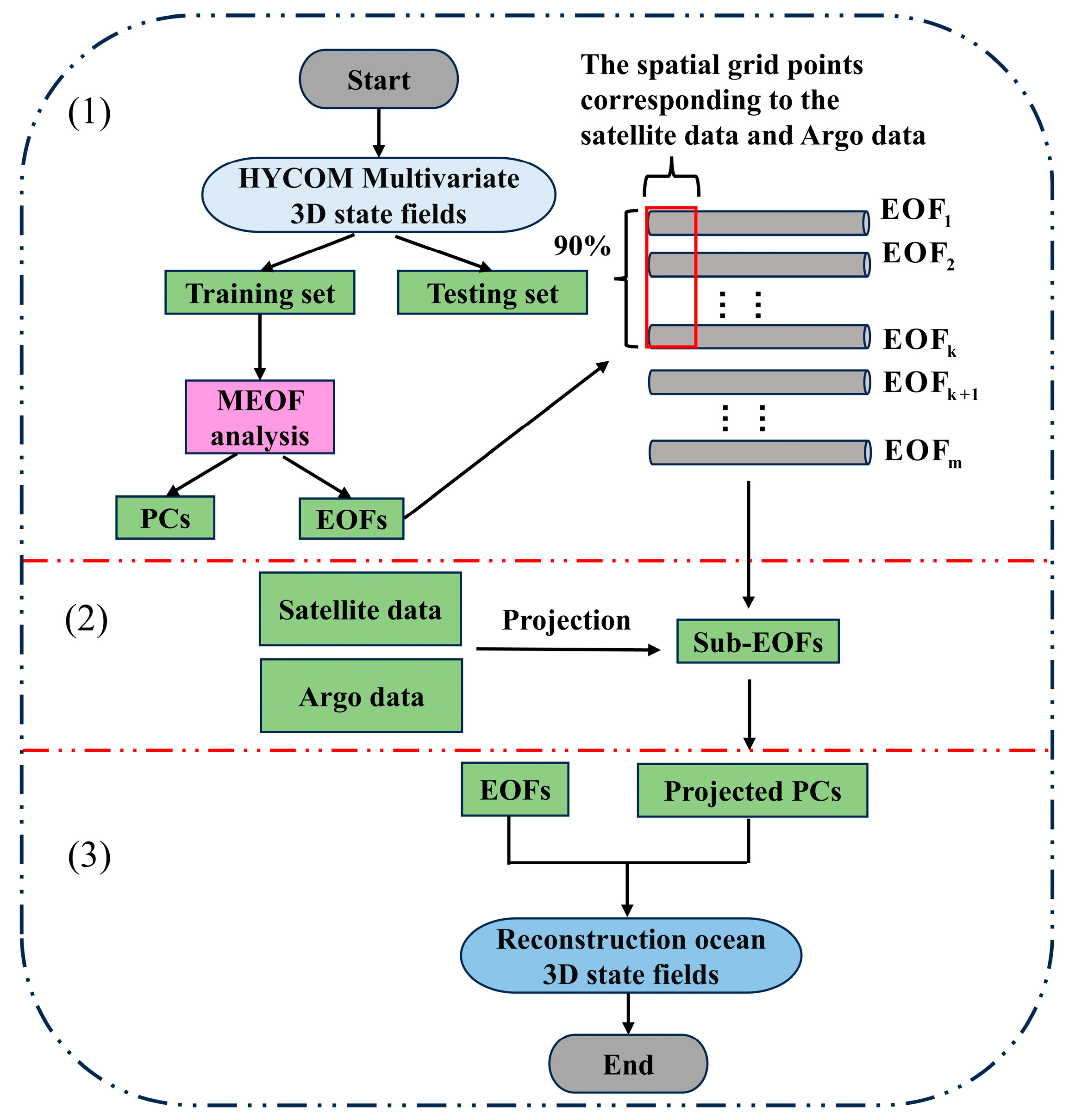
2.5. MEOF Reconstruction Framework

The MEOF method, an extension of the conventional EOF technique initially developed by Lorenz in the 1950s [34], provides a robust framework for extracting coupled empirical modes from multivariate datasets. In this study, the MEOF method was employed to examine the interrelationship among multiple marine elements and to derive dominant spatial patterns from reanalysis datasets. Through the decomposition of the reanalysis field, this method significantly reduces computational complexity while preserving essential spatial and temporal features.

The reanalysis fields of SSH, T, S, and current components (u, v) served as the background data, as mathematically represented in Equation (1). To isolate the short-term and seasonal oceanic variability, particularly the anomalous behavior of these variables, the climatological mean state was systematically removed from the background fields. Given the inherent heterogeneity in scales and units across these multivariate parameters, a standardization procedure was implemented following the method outlined in Equation (2). The resultant standardized data were subsequently organized into the sample matrix ${\mathrm{X}}^{\prime }$, which forms the basis for extracting spatial modes through MEOF.

$$\mathrm{X}=\left[\begin{array}{cccc}\mathrm{S}\mathrm{S}{\mathrm{H}}_{1,1}& \mathrm{S}\mathrm{S}{\mathrm{H}}_{1,2}& \dots & \mathrm{S}\mathrm{S}{\mathrm{H}}_{1,\mathrm{t}}\\ ⋮& ⋮& \dots & ⋮\\ \mathrm{S}\mathrm{S}{\mathrm{H}}_{{\mathrm{N}}_{\mathrm{s}\mathrm{s}\mathrm{h}},1}& \mathrm{S}\mathrm{S}{\mathrm{H}}_{{\mathrm{N}}_{\mathrm{s}\mathrm{s}\mathrm{h}},2}& \dots & \mathrm{S}\mathrm{S}{\mathrm{H}}_{{\mathrm{N}}_{\mathrm{s}\mathrm{s}\mathrm{h}},\mathrm{t}}\\ {\mathrm{T}}_{1,1}& {\mathrm{T}}_{1,2}& \dots & {\mathrm{T}}_{1,\mathrm{t}}\\ ⋮& ⋮& \dots & ⋮\\ {\mathrm{T}}_{{\mathrm{N}}_{3\mathrm{D}},1}& {\mathrm{T}}_{{\mathrm{N}}_{3\mathrm{D}},2}& \dots & {\mathrm{T}}_{{\mathrm{N}}_{3\mathrm{D}},\mathrm{t}}\\ {\mathrm{S}}_{1,1}& {\mathrm{S}}_{1,2}& \dots & {\mathrm{S}}_{1,\mathrm{t}}\\ ⋮& ⋮& \dots & ⋮\\ {\mathrm{S}}_{{\mathrm{N}}_{3\mathrm{D}},1}& {\mathrm{S}}_{{\mathrm{N}}_{3\mathrm{D}},2}& \dots & {\mathrm{S}}_{{\mathrm{N}}_{3\mathrm{D}},\mathrm{t}}\\ {\mathrm{u}}_{1,1}& {\mathrm{u}}_{1,2}& \dots & {\mathrm{u}}_{1,\mathrm{t}}\\ ⋮& ⋮& \dots & ⋮\\ {\mathrm{u}}_{{\mathrm{N}}_{3\mathrm{D}},1}& {\mathrm{u}}_{{\mathrm{N}}_{3\mathrm{D}},2}& \dots & {\mathrm{u}}_{{\mathrm{N}}_{3\mathrm{D}},\mathrm{t}}\\ \begin{array}{c}{\mathrm{v}}_{1,1}\\ ⋮\\ {\mathrm{v}}_{{\mathrm{N}}_{3\mathrm{D}},1}\end{array}& \begin{array}{c}{\mathrm{v}}_{1,2}\\ ⋮\\ {\mathrm{v}}_{{\mathrm{N}}_{3\mathrm{D}},2}\end{array}& \begin{array}{c}\dots \\ \dots \\ \dots \end{array}& \begin{array}{c}{\mathrm{v}}_{1,\mathrm{t}}\\ ⋮\\ {\mathrm{v}}_{{\mathrm{N}}_{3\mathrm{D}},\mathrm{t}}\end{array}\end{array}\right]$$

(1)

where ${\mathrm{N}}_{\mathrm{s}\mathrm{s}\mathrm{h}}={\mathrm{N}}_{\mathrm{l}\mathrm{o}\mathrm{n}}\times {\mathrm{N}}_{\mathrm{l}\mathrm{a}\mathrm{t}}$ (SSH’s horizontal grid points) and ${\mathrm{N}}_{3\mathrm{D}}={\mathrm{N}}_{\mathrm{l}\mathrm{o}\mathrm{n}}\times {\mathrm{N}}_{\mathrm{l}\mathrm{a}\mathrm{t}}\times {\mathrm{N}}_{\mathrm{d}\mathrm{e}\mathrm{p}}$ (3D grid points for T, S, u, v), with ${\mathrm{N}}_{\mathrm{l}\mathrm{o}\mathrm{n}}$, ${\mathrm{N}}_{\mathrm{l}\mathrm{a}\mathrm{t}}$, ${\mathrm{N}}_{\mathrm{d}\mathrm{e}\mathrm{p}}$ being the longitude, latitude, and depth dimensions, respectively, and with t representing the temporal dimension.

$${\mathrm{X}}^{\prime }={\mathrm{\sigma }}^{-1}(\mathrm{X}-\overline{\mathrm{X}})$$

(2)

where $\overline{\mathrm{X}}$ represents the daily mean climatology, and $\mathrm{\sigma }$ is a standardization matrix.

The sample matrix of ${\mathrm{X}}^{\prime }$ can be decomposed into the independent orthogonal spatial modes (EOFs) accompanied by their corresponding principal components (PCs), as mathematically formulated in Equation (3). This decomposition is achieved through eigenvalue analysis of the correlation coefficient matrix shown in Equation (4), where the eigenvalues (λ) and eigenvectors (V) are computed using the Jacobi iterative decomposition algorithm and $\mathrm{\Lambda }={\displaystyle \frac{1}{\mathrm{M}}}\mathrm{d}\mathrm{i}\mathrm{a}\mathrm{g}({\mathrm{\lambda }}_1,\cdots ,{\mathrm{\lambda }}_{\mathrm{t}})$, and where M is the row dimension of the X matrix, which can be expanded as $\mathrm{M}={\mathrm{N}}_{\mathrm{s}\mathrm{s}\mathrm{h}}+4{\mathrm{N}}_{3\mathrm{D}}$.

$${\mathrm{X}}^{\prime }=\mathrm{E}\mathrm{O}\mathrm{F}\mathrm{s}\cdot \mathrm{P}\mathrm{C}\mathrm{s}$$

(3)

$$\begin{array}{c}\mathrm{E}\mathrm{O}\mathrm{F}\mathrm{s}={\displaystyle \frac{1}{\sqrt{\mathrm{\lambda }}}}{\mathrm{X}}^{\prime }\mathrm{V}\\ \mathrm{P}\mathrm{C}\mathrm{s}=\sqrt{\mathrm{\lambda }}{\mathrm{V}}^{-1}\end{array}$$

(4)

$$\mathrm{C}\mathrm{o}\mathrm{r}({\mathrm{X}}^{\prime })={\displaystyle \frac{1}{\mathrm{M}}}{\mathrm{X}}^{{\prime }^{\mathrm{T}}}{\mathrm{X}}^{\prime }=\mathrm{V}\mathrm{\Lambda }{\mathrm{V}}^{\mathrm{T}}$$

(5)

where λ and V are the eigenvectors and eigenvalues of the correlation coefficient matrix $\mathrm{C}\mathrm{o}\mathrm{r}({\mathrm{X}}^{\prime })$, respectively. $\mathrm{C}\mathrm{o}\mathrm{r}({\mathrm{X}}^{\prime })$ is estimated as per Equation (5).

The derived EOFs represent stationary spatial structures that are temporally invariant and explain a substantial portion of the total variance within the multivariate dataset, whereas the temporal evolution of these patterns is encoded in the corresponding PCs. For dimensionality reduction, only those EOF modes that collectively explain 90% of the cumulative variance are retained for reconstructing the dominant spatial characteristics of the following analyzed fields.

While reanalysis data provide complete three-dimensional representations of multiple oceanic elements, they are inherently limited by their delayed availability. In contrast, satellite and buoy observations can provide real-time data streams but are restricted to surface-level variables or spatially discrete profiles. Therefore, the reconstruction framework is implemented to reconstruct a real-time three-dimensional state field of multiple variables, where spatial modes derived from reanalysis data are combined with real-time observations. This assimilation process employs the least squares approach, wherein the optimal PC is determined by minimizing the cost function as defined in Equation (6).

$$\mathrm{J}(\mathrm{P}{\mathrm{C}}_{\mathrm{p}\mathrm{r}\mathrm{o}\mathrm{j}})={\displaystyle \frac{1}{2}}{(\mathrm{E}\mathrm{O}\mathrm{F}{\mathrm{s}}_{\mathrm{I}\times \mathrm{J}}\times \mathrm{P}{\mathrm{C}}_{\mathrm{p}\mathrm{r}\mathrm{o}\mathrm{j}}-{\mathrm{X}}_{\mathrm{p}\mathrm{r}\mathrm{o}\mathrm{j}})}^{\mathrm{T}}(\mathrm{E}\mathrm{O}\mathrm{F}{\mathrm{s}}_{\mathrm{I}\times \mathrm{J}}\times \mathrm{P}{\mathrm{C}}_{\mathrm{p}\mathrm{r}\mathrm{o}\mathrm{j}}-{\mathrm{X}}_{\mathrm{p}\mathrm{r}\mathrm{o}\mathrm{j}})$$

(6)

where $\mathrm{P}{\mathrm{C}}_{\mathrm{p}\mathrm{r}\mathrm{o}\mathrm{j}}$ are the principal components obtained through projection, and ${\mathrm{X}}_{\mathrm{p}\mathrm{r}\mathrm{o}\mathrm{j}}$ represents the projection matrix. $\mathrm{E}\mathrm{O}\mathrm{F}{\mathrm{s}}_{\mathrm{I}\times \mathrm{J}}$ refers to the spatial modes in the EOFs that correspond to the spatial locations in the projection matrix. I represents the spatial dimension of the projection matrix, and J represents the number of modes selected.

Given that the variation in the elements of seawater at depths of 2000 m is minimal, this paper assumed these elements to be constant at this depth. Consequently, the bottom boundary constraints were established based on the average state of the ocean, which was incorporated in the projection matrix, as shown in Equation (7). The derivation was conducted through the minimization of the cost function, as illustrated in Equation (8).

$${\mathrm{X}}_{\mathrm{p}\mathrm{r}\mathrm{o}\mathrm{j}}={\left[\begin{array}{c}{\mathrm{X}}_{\mathrm{o}\mathrm{b}\mathrm{s}}\\ {\mathrm{X}}_{\mathrm{b}\mathrm{o}\mathrm{t}\mathrm{t}\mathrm{o}\mathrm{m}}\end{array}\right]}_{\mathrm{I}\times {\mathrm{t}}_1}$$

(7)

where ${\mathrm{t}}_1$ is the temporal dimension, and ${\mathrm{X}}_{\mathrm{o}\mathrm{b}\mathrm{s}}$ indicates selected observational data.

It is noted that different ${\mathrm{X}}_{\mathrm{o}\mathrm{b}\mathrm{s}}$ values were utilized in the testing and practical scenarios. In the testing scenario, independent data from HYCOM were assumed to be the observations, whereas in the practical scenario, real observations were employed. The details are described in the following Section 2.6.

$$\begin{array}{c}{\nabla }_{\mathrm{P}{\mathrm{C}}_{\mathrm{p}\mathrm{r}\mathrm{o}\mathrm{j}}}\mathrm{J}(\mathrm{P}{\mathrm{C}}_{\mathrm{p}\mathrm{r}\mathrm{o}\mathrm{j}})={\mathrm{E}\mathrm{O}\mathrm{F}\mathrm{s}}_{\mathrm{I}\times \mathrm{J}}{}_{ }{}^{\mathrm{T}}\mathrm{E}\mathrm{O}\mathrm{F}\mathrm{s}_{\mathrm{I}\times \mathrm{J}}^{ }\mathrm{P}{\mathrm{C}}_{\mathrm{p}\mathrm{r}\mathrm{o}\mathrm{j}}-\mathrm{E}\mathrm{O}\mathrm{F}{\mathrm{s}}_{\mathrm{I}\times \mathrm{J}}{}_{ }{}^{\mathrm{T}}\mathrm{X}_{\mathrm{p}\mathrm{r}\mathrm{o}\mathrm{j}}^{ }=0\\ \mathrm{P}{\mathrm{C}}_{\mathrm{p}\mathrm{r}\mathrm{o}\mathrm{j}}={(\mathrm{E}\mathrm{O}\mathrm{F}{\mathrm{s}}_{\mathrm{I}\times \mathrm{J}}{}_{ }{}^{\mathrm{T}}\mathrm{E}\mathrm{O}\mathrm{F}\mathrm{s}_{\mathrm{I}\times \mathrm{J}}^{ })}^{-1}\mathrm{E}\mathrm{O}\mathrm{F}{\mathrm{s}}_{\mathrm{I}\times \mathrm{J}}{}_{ }{}^{\mathrm{T}}\mathrm{X}_{\mathrm{p}\mathrm{r}\mathrm{o}\mathrm{j}}^{ }\end{array}$$

(8)

It is important to note that when projecting, the vectors in EOFs must be selected correspond to ${\mathrm{X}}_{\mathrm{p}\mathrm{r}\mathrm{o}\mathrm{j}}$ appropriately. For instance, when ${\mathrm{X}}_{\mathrm{p}\mathrm{r}\mathrm{o}\mathrm{j}}$ includes SSH, the associated EOFs must pertain specifically to the corresponding SSH components. Consequently, the spatial modes involved in Equation (8) ${\mathrm{E}\mathrm{O}\mathrm{F}\mathrm{s}}_{\mathrm{I}\times \mathrm{J}}$ represent the relevant subsets of $\mathrm{E}\mathrm{O}\mathrm{F}\mathrm{s}$. Ultimately, the estimated time series $\mathrm{P}{\mathrm{C}}_{\mathrm{p}\mathrm{r}\mathrm{o}\mathrm{j}}$ and the corresponding spatial modes can be utilized to construct the integrated three-dimensional element fields. As mentioned before, the long-term climate state was removed from the training data; therefore, the average ocean state that was excluded must be incorporated when reconstructing the state field. The integrated state field can be reconstructed as demonstrated in Equation (9).

$${\mathrm{X}}_{\mathrm{r}\mathrm{e}\mathrm{f}}=\mathrm{\sigma }(\mathrm{EOFs}\times \mathrm{P}{\mathrm{C}}_{\mathrm{p}\mathrm{r}\mathrm{o}\mathrm{j}})+\overline{\mathrm{X}}$$

(9)

In summary, the MEOF reconstruction framework comprises three components, as illustrated in Figure 3: multivariate joint decomposition, satellite and Argo data projection, and reconstruction integration. The functions of each component are defined as follows:

(1)

Multivariate joint decomposition: the MEOF method is applied to decompose multivariate ocean fields into EOFs, from which sub-EOFs explaining 90% of the variance and corresponding to satellite and Argo data are selected.

(2)

Satellite and Argo data projection: satellite and Argo data are projected onto the selected sub-EOFs to derive the projected PCs.

(3)

Reconstruction integration: the complete EOFs are combined with the projected PCs to generate 3D reconstructed ocean fields.

Figure 3. The flowchart of the MEOF reconstruction framework.

Figure 3. The flowchart of the MEOF reconstruction framework.

2.6. Design of Experiments

To assess the effectiveness of the proposed framework, two experimental scenarios were designed: the testing scenario and the practical scenario. In the testing scenario, the ocean element reconstruction schemes were evaluated and validated. The optimal scheme identified during this phase was subsequently applied in the practical scenario to reconstruct the actual ocean state field.

In this testing scenario, only HYCOM reanalysis data were utilized. The data from 1996 to 2016 served as the training data for constructing the spatial modes, while the SSH, SST, and SSS data from HYCOM in 2017 were treated as observational inputs for ocean state reconstruction. The remaining data from 2017 were reserved for validation purposes and excluded from the reconstruction process. To evaluate the influence of each observed element on the reconstruction of the ocean state field, the observational data were combined sequentially and utilized for reconstruction, as tested in Experiments 1–3 outlined in

Table 1. Setup of different experiments.

Experiment	Spatial Modes	Projection Matrix	Validation Data
Exp. 1 1	$\left(\mathrm{a}\right) \mathrm{E}\mathrm{O}{\mathrm{F}}_{\mathrm{S}\mathrm{S}\mathrm{H}}$$, \left(\mathrm{b}\right) \mathrm{E}\mathrm{O}{\mathrm{F}}_{\mathrm{S}\mathrm{S}\mathrm{T}}$$, \left(\mathrm{c}\right) \mathrm{E}\mathrm{O}{\mathrm{F}}_{\mathrm{S}\mathrm{S}\mathrm{S}}$	${\mathrm{X}}_{\mathrm{o}\mathrm{b}\mathrm{s}}$$\text{:} \left(\mathrm{a}\right) \mathrm{H}\mathrm{Y}\mathrm{C}\mathrm{O}{\mathrm{M}}_{\mathrm{S}\mathrm{S}\mathrm{H}}$$, \left(\mathrm{b}\right) \mathrm{H}\mathrm{Y}\mathrm{C}\mathrm{O}{\mathrm{M}}_{\mathrm{S}\mathrm{S}\mathrm{T}}$$, \left(\mathrm{c}\right) \mathrm{H}\mathrm{Y}\mathrm{C}\mathrm{O}{\mathrm{M}}_{\mathrm{S}\mathrm{S}\mathrm{S}}$	HYCOM data for 2017, including T, S, u, and v
Exp. 2	$\left(\mathrm{a}\right) [\mathrm{E}\mathrm{O}{\mathrm{F}}_{\mathrm{S}\mathrm{S}\mathrm{H}}$$,\mathrm{E}\mathrm{O}{\mathrm{F}}_{\mathrm{S}\mathrm{S}\mathrm{T}}],$ $\mathrm{b}) [\mathrm{E}\mathrm{O}{\mathrm{F}}_{\mathrm{S}\mathrm{S}\mathrm{H}}$$,\mathrm{E}\mathrm{O}{\mathrm{F}}_{\mathrm{S}\mathrm{S}\mathrm{S}}],$ $\left(\mathrm{c}\right) [\mathrm{E}\mathrm{O}{\mathrm{F}}_{\mathrm{S}\mathrm{S}\mathrm{T}}$$,\mathrm{E}\mathrm{O}{\mathrm{F}}_{\mathrm{S}\mathrm{S}\mathrm{S}}$]	${\mathrm{X}}_{\mathrm{o}\mathrm{b}\mathrm{s}}$$\text{:} \left(\mathrm{a}\right) [\mathrm{H}\mathrm{Y}\mathrm{C}\mathrm{O}{\mathrm{M}}_{\mathrm{S}\mathrm{S}\mathrm{H}}$$, \mathrm{H}\mathrm{Y}\mathrm{C}\mathrm{O}{\mathrm{M}}_{\mathrm{S}\mathrm{S}\mathrm{T}}],$ $\left(\mathrm{b}\right) [\mathrm{H}\mathrm{Y}\mathrm{C}\mathrm{O}{\mathrm{M}}_{\mathrm{S}\mathrm{S}\mathrm{H}}$$, \mathrm{H}\mathrm{Y}\mathrm{C}\mathrm{O}{\mathrm{M}}_{\mathrm{S}\mathrm{S}\mathrm{S}}],$ $\left(\mathrm{c}\right) [\mathrm{H}\mathrm{Y}\mathrm{C}\mathrm{O}{\mathrm{M}}_{\mathrm{S}\mathrm{S}\mathrm{T}}$$, \mathrm{H}\mathrm{Y}\mathrm{C}\mathrm{O}{\mathrm{M}}_{\mathrm{S}\mathrm{S}\mathrm{S}}$]
Exp. 3	$[\mathrm{E}\mathrm{O}{\mathrm{F}}_{\mathrm{S}\mathrm{S}\mathrm{H}}$$, \mathrm{E}\mathrm{O}{\mathrm{F}}_{\mathrm{S}\mathrm{S}\mathrm{T}}$$, \mathrm{E}\mathrm{O}{\mathrm{F}}_{\mathrm{S}\mathrm{S}\mathrm{S}}$]	${\mathrm{X}}_{\mathrm{o}\mathrm{b}\mathrm{s}}$$\text{:} [\mathrm{H}\mathrm{Y}\mathrm{C}\mathrm{O}{\mathrm{M}}_{\mathrm{S}\mathrm{S}\mathrm{H}}$$, \mathrm{H}\mathrm{Y}\mathrm{C}\mathrm{O}{\mathrm{M}}_{\mathrm{S}\mathrm{S}\mathrm{T}}$$, \mathrm{H}\mathrm{Y}\mathrm{C}\mathrm{O}{\mathrm{M}}_{\mathrm{S}\mathrm{S}\mathrm{S}}$]
Exp. 4	The optimal scheme	$\mathrm{The} \mathrm{optimal} \mathrm{scheme} \mathrm{and} {\mathrm{X}}_{\mathrm{o}\mathrm{b}\mathrm{s}}$: satellite data	Argo data for 2017, including T and S
Exp. 5	The optimal scheme	$\mathrm{The} \mathrm{optimal} \mathrm{scheme} \mathrm{and} {\mathrm{X}}_{\mathrm{o}\mathrm{b}\mathrm{s}}$: satellite data and Argo data

¹ Exp is ‘Experiment’.

. In Experiment 1, three separate tests were conducted using SSH, SST, and SSS individually as observations in the projection matrix to be extended and reconstruct the integrated ocean state field. Experiment 2 combined the three observational variables—SSH, SST and SSS—in pairs and used them as the observations in the projection matrix to perform three sets of tests. Experiment 3 employed all three observational variables simultaneously. Through these experiments, the optimal reconstruction scheme was determined and subsequently applied to real observational information in the practical scenario for Experiments 4–5.

In Experiment 4, satellite remote sensing data from 2017 were used as observations, and the results were validated against the Argo float observations from the same year. Additionally, discrete Argo observations were incorporated in Experiment 5 to evaluate their impact on the vertical variation in the reconstruction results. A period with a relatively high number of Argo profiles, from 8 March to 14 March 2017, was selected. During this period, 14 profiling observations were available, of which 12 datasets were utilized for reconstruction, while 2 datasets were reserved for independent validation.

3. Results

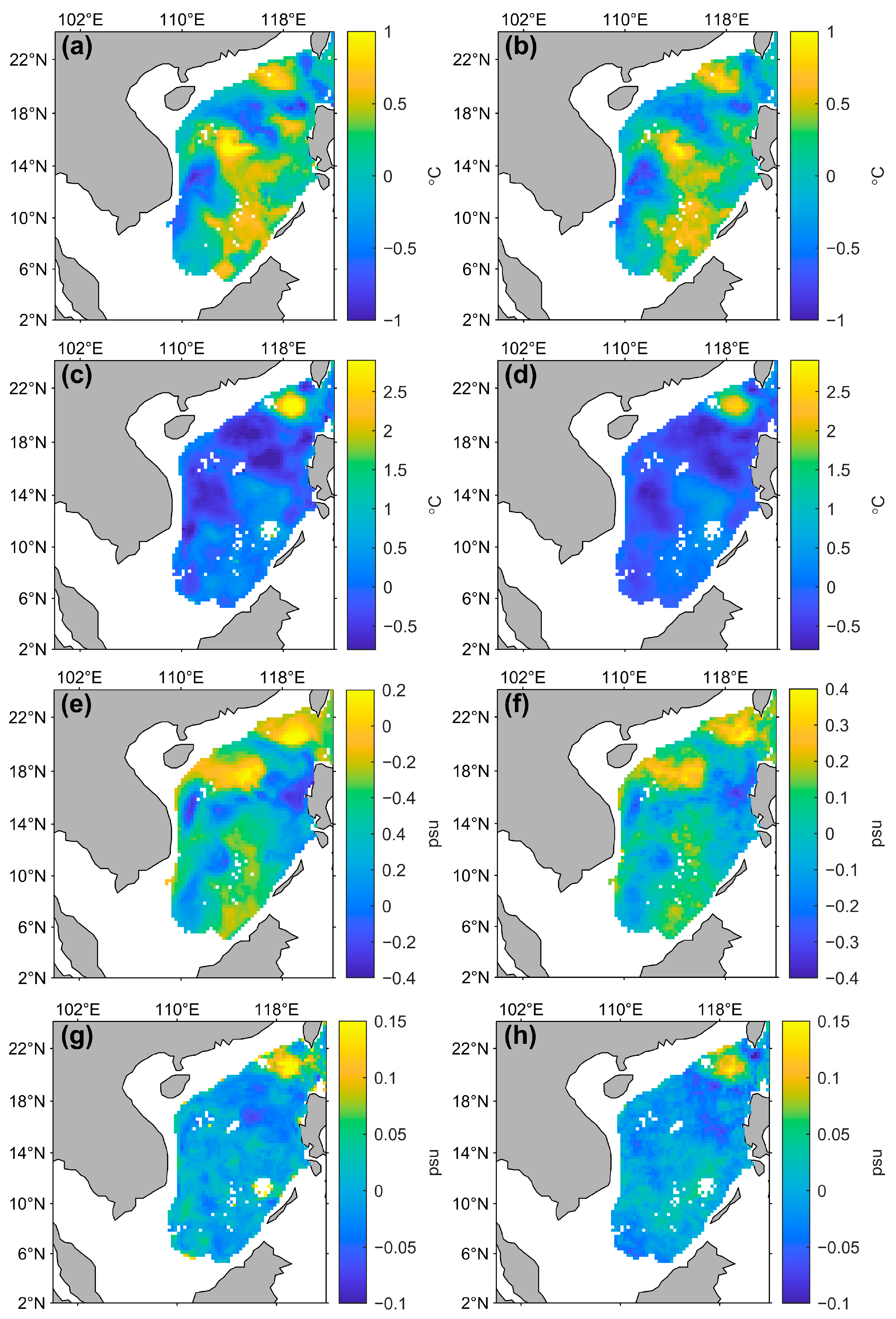
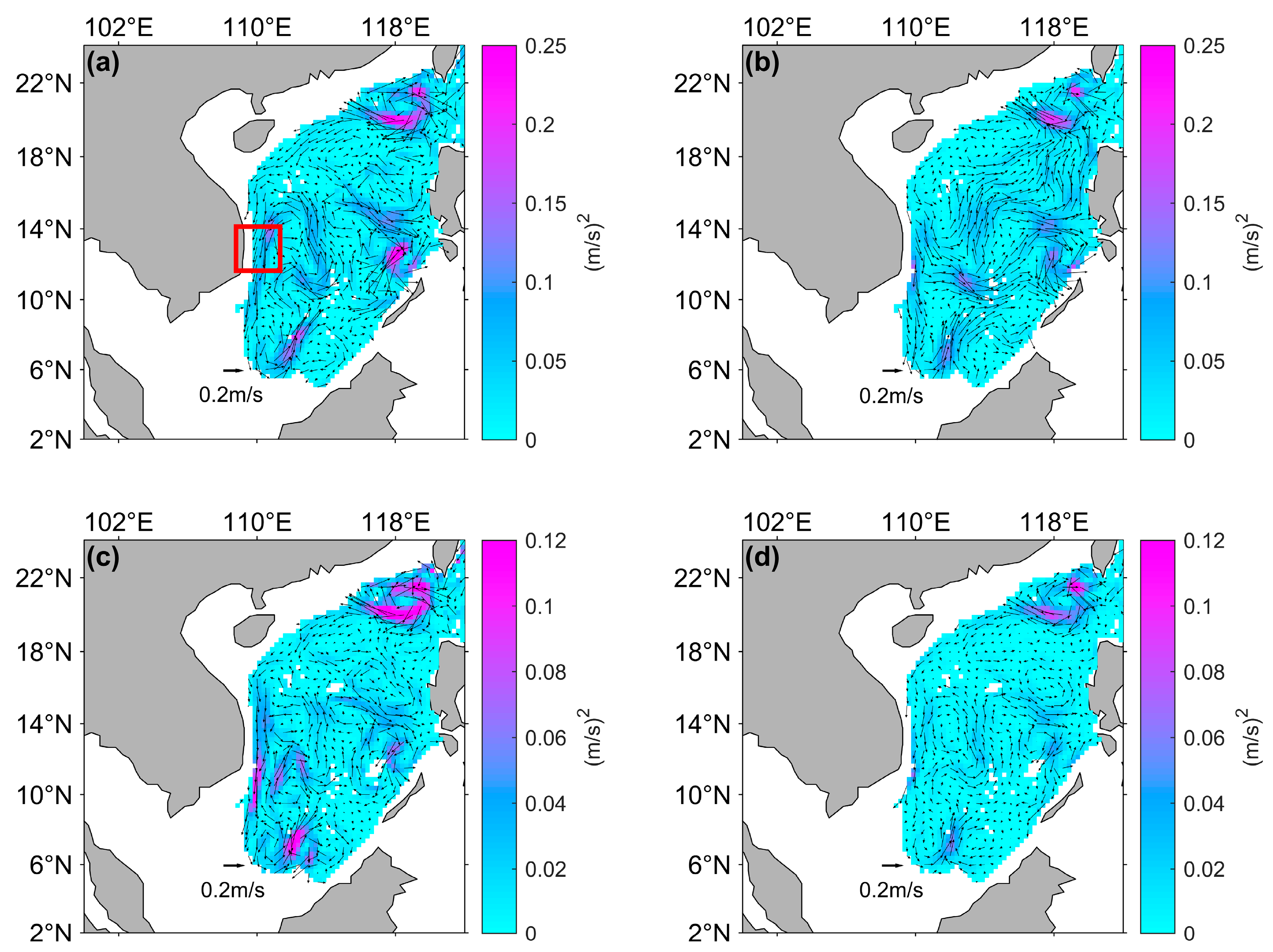
3.1. Testing Experiment

The reconstructed state fields for various oceanic elements were statistically evaluated using the root mean square error (RMSE), as described in Equation (10).

$$\mathrm{R}\mathrm{M}\mathrm{S}{\mathrm{E}}_{\mathrm{z}}=\sqrt{{\displaystyle \frac{{\displaystyle \sum _{\mathrm{i}=1}^{{\mathrm{t}}_1}{\displaystyle \sum _{\mathrm{j}=1}^{{\mathrm{r}}_1}({\mathrm{L}}_{\mathrm{i},\mathrm{j},\mathrm{z}}-{\mathrm{P}}_{\mathrm{i},\mathrm{j},\mathrm{z}})}}}{{\mathrm{t}}_1\times {\mathrm{r}}_1}}}$$

(10)

where $\mathrm{R}\mathrm{M}\mathrm{S}{\mathrm{E}}_{\mathrm{z}}$ represents the RMSE value of the ${\mathrm{z}}^{\mathrm{t}\mathrm{h}}$ layer; ${\mathrm{L}}_{\mathrm{i},\mathrm{j},\mathrm{z}}$ and ${\mathrm{P}}_{\mathrm{i},\mathrm{j},\mathrm{z}}$ are the truth and reconstructed value of the ${\mathrm{j}}^{\mathrm{t}\mathrm{h}}$ grid points and ${\mathrm{z}}^{\mathrm{t}\mathrm{h}}$ layer in the ${\mathrm{i}}^{\mathrm{t}\mathrm{h}}$ day, respectively; and ${\mathrm{t}}_1$ and ${\mathrm{r}}_1$ are the temporal dimension and spatial dimension of the testing data, respectively.

The reconstructed state fields from Experiments 1–3 were compared with independent HYCOM testing datasets. Statistical results for temperature, salinity, and currents within the upper 1000 m are presented in Figure 4. For the temperature reconstruction, all experiments exhibited lower errors in the upper 100 m. However, the reconstruction performance deteriorated around the 100 m depth due to the presence of the thermocline. Below this depth, the error in the reconstructed field decreased significantly, attributed to the influence of the bottom boundary condition established. Among these experiments, schemes utilizing SST as a reconstruction input—specifically, Exp. 1(b), Exp. 2(a), Exp. 2(c), and Exp. 3—demonstrated notably better performance in the upper 10 m, with an RMSE of approximately 0.3 °C. This was expected, as shallow water temperatures are strongly related to the observed SST. However, as depth increased, the performance of Exp. 1(b) declined rapidly, with the RMSE rising to 1.7 °C around the 100 m depth. In contrast, schemes incorporating SSH as the input, such as Exp. 1(a), Exp. 2(a), Exp. 2(b), and Exp. 3, exhibited lower errors, with an RMSE of approximately 1.3 °C at the thermocline and even lower values at greater depths. This indicates that SSH plays a crucial role in estimating the temperature, particularly in deeper waters, consistent with the findings of Guinehut et al. [35]. These results highlight that the influence of the surface temperature is largely confined to the upper 60 m, while SSH contributes significantly to temperature estimation in deeper regions. Additionally, SSS does not significantly impact the reconstruction of either surface or deep temperatures, as evidenced by the results from Exp. 1(c). Therefore, considering the results from the surface to a 1000 m depth, the optimal scheme for temperature reconstruction involves the use of SSH and SST observations as the projection matrix (Exp. 2(a)).

The salinity reconstruction followed a similar trend, as illustrated in Figure 4b. The experiments incorporating SSS (Exp. 1(c), Exp. 2(b), Exp. 2(c), and Exp. 3) accurately reproduced the salinity, with errors limited to less than 0.1 psu. In contrast, the experiments excluding SSS exhibited larger errors, approximately 0.25 psu. The effectiveness of SSS-inclusive experiments decreased with increasing depth, with errors rising to approximately 0.35 psu at the 100 m pycnocline. This suggests that the integration of SSS significantly enhances the reconstruction accuracy in the surface and subsurface layers, although its influence diminishes beneath the pycnocline. Notably, while all experiments exhibited peak errors near the pycnocline, Exp. 3 maintained a slight superiority, demonstrating the smallest error, albeit not significantly. Therefore, these findings imply that incorporating additional variables is beneficial for the salinity reconstruction process. For the most accurate salinity reconstruction, the optimal scheme combines SSH, SST, and SSS as observational inputs in the projection matrix, as exemplified by Exp. 3.

In the reconstruction of ocean currents, as illustrated in Figure 4c,d, the exclusion of SSH leads to a relatively higher error, with surface current discrepancies exceeding 0.25 m/s, which gradually decrease with depth. An analysis of the results from Exp. 1(a), Exp. 2(a), Exp. 2(b), and Exp. 3 indicates that the utilization of SSH data alone yields a minimal error margin. This finding highlights the critical role of SSH in enhancing the accuracy of the reconstructed current components (u, v). Therefore, the observed SSH data were selected as the sole input for reconstructing the current field, as demonstrated in Exp. 1(a).

Reflecting on the implications of the aforementioned experiments, it is evident that the reconstruction of each oceanographic element is influenced by various observational datasets and their corresponding spatial modes, with each element following a distinct methodological framework. The optimal experimental schemes for reconstructing each element are summarized in

Table 2. The optimal experimental schemes for each element.

Elements	Spatial Modes	Projection Matrix
T	[$\mathrm{E}\mathrm{O}{\mathrm{F}}_{\mathrm{S}\mathrm{S}\mathrm{H}}$, $\mathrm{E}\mathrm{O}{\mathrm{F}}_{\mathrm{S}\mathrm{S}\mathrm{T}}$]	[SSH, SST]
S	[$\mathrm{E}\mathrm{O}{\mathrm{F}}_{\mathrm{S}\mathrm{S}\mathrm{H}}$, $\mathrm{E}\mathrm{O}{\mathrm{F}}_{\mathrm{S}\mathrm{S}\mathrm{T}}$, $\mathrm{E}\mathrm{O}{\mathrm{F}}_{\mathrm{S}\mathrm{S}\mathrm{S}}$]	[SSH, SST, SSS]
u and v	$\mathrm{E}\mathrm{O}{\mathrm{F}}_{\mathrm{S}\mathrm{S}\mathrm{H}}$	SSH

.

To further illustrate a spatial representation of the reconstructed results, temporally averaged reconstructed state fields were calculated. Taking the temperature and salinity as examples, the reconstructed results at depths of 10 m and 300 m were compared with the temporal averages of the original HYCOM data at the same depths, as shown in Figure 5a–d. As observed, the reconstructed temperature effectively reproduced the distribution characteristics of the original HYCOM temperature field in both the shallow layer at 10 m and the deep layer at 300 m. Furthermore, the warm eddy in the northern part of the South China Sea was also captured across various depths, although a slight underestimation was observed in the reconstruction. A similar finding is evident in the reconstructed salinity field, as shown in Figure 5e–h, where the generated salinity field closely replicated the significant spatial variations present in the HYCOM ocean salinity field.

The temporal averages of the reconstructed current fields and kinetic energies (KEs) at the surface and deep layers near the pycnocline are presented in Figure 6, alongside the original HYCOM data for comparative analysis. It is important to note that in order to maintain consistency with actual satellite observations, HYCOM ocean current data were not employed as observations in the projection matrix in these testing experiments. Instead, all the reconstructed ocean currents were derived from the derived spatial modes and the information transferred based on satellite data. As shown in Figure 6a,b, the reconstructed surface current fields exhibited spatial distributions closely aligned with those of the HYCOM surface layer currents. The magnitude and direction of the currents across most of our study area, particularly in the northern and southern regions, were accurately reproduced. However, in the vicinity of (110°E, 14°N), the eddies apparent in the reanalysis field were less distinct in the reconstructed field results. Regarding kinetic energy, the reconstructed kinetic energy field was slightly lower than that from the HYCOM data, yet both displayed comparable spatial distribution patterns. This indicates that the reconstructed field successfully captures the primary features of the original ocean state, with temperature, salinity, and current distributions effectively restored in space.

These findings underscore the reliability of our proposed reconstruction approach, which demonstrates high accuracy and robustness. This methodological framework makes it easier to apply in further experiments that involve reconstructing actual observational data. It can reasonably extend observational information in both time and space.

3.2. Practical Experiments

3.2.1. Reconstruction Based on Satellite Observation Dataset

Based on the results from the aforementioned experiments, various oceanic elements can be estimated based on distinct observational matrix schemes. In these practical experiments, the spatial modes were stored and employed to extend the actual satellite observation dataset, as summarized in Table 2. To validate the reliability of the reconstructed results, actual observations from Argo profiling floats were extracted for comparative analysis. The RMSE of the reconstructed field was calculated based on Equation (10), where L represents the Argo observations, and P denotes the reconstructed field. Additionally, the HYCOM datasets and MODAS were also compared with the same Argo data, and their corresponding RMSE values are presented in Figure 6 for comparison.

A comparison of the temperature errors of the HYCOM reanalysis, MODAS, and the present method with the Argo in situ observations revealed that they were very similar in the 0-50 m range. However, significant discrepancies emerged in the vicinity of the thermocline (~100 m), where MODAS attained an RMSE of 2 °C at the thermocline. This finding indicates that MODAS, which is based on historical observations, is no longer adequate in describing the contemporary three-dimensional temperature structure of the ocean. In comparison to MODAS, our method demonstrated a 34% reduction in error. It is important to note that this experiment solely used satellite observations for reconstruction without incorporating in situ observations yet. This finding suggests that incorporating in situ observations will enhance the efficacy of our method. As the depth increased, the error of MODAS was still systematically higher than that of our method, which was relatively stable. The aforementioned results indicate that reasonable spatial modes are the basis for reconstructing the three-dimensional state field. Indeed, the reconstruction of the field is primarily dependent on the spatial modes extracted from HYCOM. It is acknowledged that the spatial modes provided by different reanalysis products may be somewhat divergent. However, the simplicity and efficiency of our reconstruction framework facilitate its extension to different products.

Furthermore, it was determined that satellite observations were beneficial in the reconstruction of the thermohaline structure above the thermocline (~50 m depth). However, due to the absence of constraints from in situ observations, the salinity structure reconstructed using solely satellite observations with spatial modes may contain substantial errors (Figure 7b). It is evident that the salinity error of our method was considerably smaller than that of MODAS for reconstructions shallower than 50 m. However, the error of the reconstructed salinity field around 100 m was marginally larger than that of MODAS (no more than 0.1 psu). It is evident from the preliminary testing and experimental findings that the sea surface salinity exerts a substantial influence on the underlying underwater salinity structure. The existing salinity satellite observations are subject to uncertainty [36,37], leading to discrepancies between observations and the spatial modes of the reanalysis data. This has a direct impact on the correlation of the three-dimensional modes. Consequently, it is imperative to incorporate in situ observations for the purpose of calibration in the salinity reconstruction process.

In summary, the proposed method achieved a temperature reconstruction accuracy comparable to the reanalysis products across the depths. Although the salinity errors slightly exceeded MODAS near the thermocline, superior performance persisted at other depths. This finding indicates that the proposed method is capable of generating a plausible three-dimensional temperature and salinity structure when solely relying on satellite observations. This is attributed to the synergistic relationship between multivariate spatial modes and the sea surface observations, which plays a pivotal role in the reconstruction process.

To further evaluate the method’s performance, we analyzed the mesoscale structure in the reconstruction results. In the same study region, previous researchers, i.e., Chu et al. [38], tracked the Western SCS Anticyclonic Eddy (WAE) using both in-situ and satellite observational data. Their study presents the temperature fields at various depths of the WAE from 7–13 June 2017 (see Figure 3 in Chu et al. [38]). We extracted and compared our reconstructed temperature fields for the same period with their analysis. To ensure consistency, the reconstructed temperature fields at depths of 100 m, 200 m, and 600 m, along with the current fields at 100 m, are displayed in Figure 8 and compared with the observational results from Chu et al. [38] At a depth of 100 m, the reconstructed temperature at the center of the eddy exceeded 23 °C, resulting in a temperature anomaly of more than 2.5 °C, which is consistent with the findings of Chu et al. [38] At a depth of 200 m, the temperature at the center of the eddy was approximately 17 °C, which is consistent with the observations, while the temperature anomaly was slightly lower than that reported by Chu et al. These results indicate that the reconstructed temperature field effectively reproduced the eddy structure at different depths, particularly in the shallow layers (above 100 m), although it was slightly lower than the actual observations in the deeper layers. The discrepancies in temperature anomalies may arise from the different ocean average states utilized. Chu et al. [38] employed the monthly mean from the 2013 World Ocean Atlas [39], whereas this study utilized daily means derived from reanalysis data. Furthermore, the reconstructed current fields shown in Figure 8d accurately reflect the warm eddy present in the region, aligning well with the temperature field results. These findings indicate that the reconstructed field not only reproduces the spatial distribution characteristics of the reanalysis field, which are comparable to actual observations, but also captures real ocean phenomena such as eddies. This further confirms the effectiveness of our proposed reconstruction framework.

3.2.2. Integration of Argo Observation Profiles in Projections

As previously discussed, the surface satellite data significantly influenced the reconstruction results within the upper 100 m. To investigate whether incorporating Argo profile data, which provide information at various depths, could enhance the reconstruction accuracy in deeper regions, Experiment 5 was conducted, as outlined earlier. This study focused on the region bounded by 12°N–24°N and 110°E–122°E, where 14 Argo data points are available. Of these, 86% were incorporated as the input for the reconstruction observations, while the remaining 14% were reserved exclusively for validation, as illustrated in Figure 9. The reconstruction results were then compared with independent Argo observations. For comparative analysis, the results from Experiment 4, which excluded the Argo data, are also presented in Figure 9.

As shown in Figure 9b, discrepancies existed between the reconstructed field and Argo observations at depths of 50–150 m, but the incorporation of the Argo profile data reduced these errors. Meanwhile, Figure 9d reveals that the inclusion of surrounding Argo profiles did not significantly alter the reconstructed temperature field, which already aligned well with observations. At depths of 200 m, the addition of adjacent Argo profiles brought the reconstruction closer to the measurements, though this effect remained relatively minor. This is likely because the spatial modes and sea surface satellite observations contain adequate information to reconstruct the vertical temperature structure of the ocean accurately.

As shown in Figure 9c,e, both Experiment 4 and Experiment 5 exhibited high accuracy in the salinity field reconstruction within the upper 50 m layer, achieving a precision comparable to the independent salinity measurements at the validation test points. However, near the 100 m thermocline, Experiment 4 exhibited discrepancies between the reconstructed and observed salinity values. In contrast, the synergistic integration of vertical profile data into the observation matrix in Experiment 5 substantially mitigated errors near the thermocline. At greater depths, the salinity reconstruction errors in Experiment 5 remained smaller than those in Experiment 4 at the (17.95°N, 118.82°E) test site, whereas limited improvement was observed at (15.67°N, 114.74°E). This likely stems from the closer proximity of the (17.95°N, 118.82°E) site to neighboring observational profiles. These salinity experiments confirm that assimilating the profile observations effectively calibrates sea surface data uncertainties, particularly enhancing the reconstruction precision near the thermocline. Nevertheless, the magnitude of the improvement depends critically on the spatial density of surrounding profiles, their geospatial proximity to target grid points, and the inter-profile correlation characteristics.

4. Discussion

This study developed a reconstruction framework based on the MEOF method. By deriving spatial modes from historical reanalysis data to characterize multivariate interactions, the framework then integrates satellite-derived surface parameters (SSHA, SST, and SSS) with in situ Argo float profiles. This integration enables real-time three-dimensional oceanic field reconstruction while preserving intrinsic physical relationships among the temperature, salinity, and current fields. Compared to the widely implemented MODAS system in operational applications, our framework demonstrates superior reconstruction accuracy, showing significant potential for operational oceanography deployments.

The reconstruction framework was validated through experiments in the South China Sea. The results demonstrate that the synergistic interaction between SSH and SST provides critical constraints for subsurface temperature reconstruction. This synergy stems from their complementary dynamical roles: SSH captures baroclinic modes governing subsurface thermal structures through geostrophic coupling, while SST directly modulates thermodynamic processes in the mixed layer. Notably, SSS is excluded from the temperature reconstruction, as salinity variations contribute minimally to density gradients in open-ocean regions. This exclusion allows the system to focus on thermally dominated processes. The optimal current field reconstruction achieved using SSH alone reveals the inherent limitations of the MEOF method—as a linear statistical framework—in capturing nonlinear signals. By leveraging statistical covariance between historical SSH and temperature/salinity (T/S) profiles, MEOF effectively characterizes geostrophic dynamics from surface to subsurface layers. However, due to lacking explicit momentum equation constraints and relying solely on historical data, while MEOF can partially reflect non-geostrophic currents through long-term statistical relationships, its modal decomposition inherently filters out most non-geostrophic signals. This limitation restricts its responsiveness to anomalous forcings, such as typhoon-induced wind-driven currents. Future implementations could integrate satellite-derived surface current products (e.g., Ocean Surface Current Analyses Real-time [OSCAR]) to introduce real-time kinematic constraints, thereby enhancing the framework’s ability to resolve transient currents.

While our results are derived from HYCOM reanalysis data, the MEOF method’s reliance on covariance structures implies that datasets sharing core physical equations and observational constraints (e.g., Simple Ocean Data Assimilation [SODA], Global Ocean Reanalysis System [GLORYS]) will produce qualitatively similar dominant modes. Secondary modes may exhibit variations due to resolution limitations or region-specific assimilation strategies, but these differences do not compromise our principal conclusions. Furthermore, transitioning between reanalysis datasets in operational applications is a straightforward process due to the method’s computational efficiency. The MEOF framework can readily utilize higher-accuracy reanalysis products when available, thereby enhancing reconstruction precision.

In practical experiments, the proposed MEOF reconstruction framework demonstrates near-real-time three-dimensional oceanic state reconstruction through synergistic use of satellite and in situ observational data. However, several challenges in operational applications require attention. First, current near-real-time SSHA products have a 3–5-day latency, limiting true real-time reconstruction capabilities. Second, systematic errors exist between satellite and in situ measurements, particularly for SSS. As demonstrated by Boutin et al. [36], these inherent discrepancies arise from near-surface stratification and sub-footprint variability. Comparisons between satellite and Argo SSS data show a root mean square deviation (RMSD) of approximately 0.2 psu in open-ocean areas, with significantly larger deviations in coastal regions [37]. These systematic biases partially explain the higher errors in thermocline salinity reconstruction compared to Argo data. Third, in situ observations remain insufficient in the South China Sea (as shown in Figure 2 and Figure 9). Although incorporating profile observations improves the accuracy of subsurface reconstructions to some extent, their impact remains limited when observations are spatially sparse. Improvements are more pronounced when reconstruction areas are near observation profiles or when surface data contain inaccuracies; otherwise, the enhancement may be negligible. Under sparse in situ observations, the primary factors influencing the reconstruction accuracy are the spatial modes from reanalysis data and satellite data. These operational limitations highlight the necessity of continuously advancing ocean observation systems to fully realize the potential of the MEOF framework in operational oceanography.

The current MEOF reconstruction framework demonstrates a high computational efficiency that aligns with operational requirements. In this study, eigenvalue decomposition of our spatiotemporal matrix required only 173 s on a Dell workstation (Precision Tower 3431, Xiamen, China) equipped with an Intel Core i9-9900 processor (8 cores/16 threads) and 64GB DDR4 RAM, with the majority of the computation time spent on the eigenvalue decomposition phase. To extend this method to larger or dynamically complex regions, we recommend employing parallel EOF analysis [40] for processing large-scale matrices. This approach enables efficient large-scale three-dimensional field reconstruction through distributed computing architectures.

This framework provides some references for AI-based reconstruction research; looking ahead, combining physical modes with observational data will offer valuable guidance for studies in this field.

5. Conclusions

This study addresses the critical need for accurate and timely reconstruction of ocean state fields by proposing a reconstruction framework based on the MEOF method. By deriving spatial modes from reanalysis data, this approach effectively integrates satellite data and Argo data to reconstruct a three-dimensional ocean state field, including temperature, salinity, and current fields. The method was tested in the South China Sea, with key findings from the testing experiments indicating that SSH and SST are essential for accurate temperature reconstruction, while SSS significantly enhances salinity estimates. Notably, current fields are most effectively reconstructed using SSH alone. These results highlight that optimal reconstruction of ocean state fields is not achieved by simply aggregating all oceanic elements into an observation matrix. Instead, each element exhibits distinct sensitivities to specific observational variables and their associated spatial modes, necessitating tailored input selection for the reconstruction model.

Practical experiments further validate the reliability of the proposed scheme, demonstrating that the reconstructed fields exhibit strong agreement with independent Argo observations, outperforming traditional baseline methods and effectively capturing the vertical structure of ocean eddies. The incorporation of Argo profiles as an input for the reconstruction model enhances the salinity reconstruction near the thermocline. In cases where surface observation data are inaccurate, the inclusion of profile data effectively corrects errors arising from these inaccuracies. However, improvements are more pronounced in regions close to the observed profile locations. The primary influence on the reconstruction accuracy remains the spatial modes derived from reanalysis data and real-time surface information from satellite observations, emphasizing the necessity for high-quality surface data and robust spatial modes.

Since the spatial modes can be pre-generated and preserved based on historical reanalysis data, the reconstruction of the entire ocean state fields can be promptly executed upon the availability of real-time satellite data. Overall, the proposed reconstruction framework offers a computationally efficient and reliable approach for reconstructing ocean state fields, making it well suited for operational forecasting and real-time applications. This framework not only advances ocean state estimation but also supports further operational forecasting efforts.

References

1. Li, Q.Y.; Sun, L.; Liu, S.S.; Xian, T.; Yan, Y.F. A new mononuclear eddy identification method with simple splitting strategies. Remote Sens. Lett. 2014, 5, 65–72. [Google Scholar] [CrossRef]
2. Li, Q.Y.; Sun, L.; Lin, S.F. GEM: A dynamic tracking model for mesoscale eddies in the ocean. Ocean Sci. 2016, 12, 1249–1267. [Google Scholar] [CrossRef]
3. Chelton, D.B.; Schlax, M.G.; Samelson, R.M. Global observations of nonlinear mesoscale eddies. Prog. Oceanogr. 2011, 91, 167–216. [Google Scholar] [CrossRef]
4. Chen, G.; Gan, J.; Xie, Q.; Chu, X.Q.; Wang, D.X.; Hou, Y.J. Eddy heat and salt transports in the South China Sea and their seasonal modulations. J. Geophys. Res. Oceans 2012, 117, C05021. [Google Scholar] [CrossRef]
5. Shao, Q.; Li, W.; Hou, G.C.; Han, G.J.; Wu, X.B. Mid-Term simultaneous spatiotemporal prediction of sea surface height anomaly and sea surface temperature using satellite data in the south China sea. IEEE Geosci. Remote Sens. Lett. 2020, 19, 1–5. [Google Scholar] [CrossRef]
6. Shao, Q.; Li, W.; Han, G.J.; Hou, G.C.; Liu, S.Y.; Gong, Y.T.; Qu, P. A deep learning model for forecasting sea surface height anomalies and temperatures in the south China sea. J. Geophys. Res. Oceans 2021, 126, e2021JC017515. [Google Scholar] [CrossRef]
7. Hu, S.; Shao, Q.; Li, W.; Han, G.J.; Zheng, Q.Y.; Wang, R.; Liu, H.Y. Multivariate sea surface prediction in the Bohai sea using a data-driven model. J. Mar. Sci. Eng. 2023, 11, 2096. [Google Scholar] [CrossRef]
8. Hurlburt, H.E. The potential for ocean prediction and role of altimeter data. Mar. Geod. 1984, 8, 17–66. [Google Scholar] [CrossRef]
9. Hurlburt, H.E. Dynamic transfer of simulated altimeter data into subsurface information by a numerical ocean model. J. Geophys. Res. Oceans 1986, 91, 2372–2400. [Google Scholar] [CrossRef]
10. Zhu, Y.H.; Cao, G.J.; Wang, Y.G.; Li, S.J.; Xu, T.F.; Wang, D.Q.; Teng, F.; Wei, Z.X. Variability of the deep South China Sea circulation derived from HYCOM reanalysis data. Acta Oceanol. Sin. 2022, 41, 54–64. [Google Scholar] [CrossRef]
11. Wang, M.; Liu, Z.J.; Zhu, X.H.; Yan, X.M.; Zhang, Z.Z.; Zhao, R.X. Origin and formation of the Ryukyu Current revealed by HYCOM reanalysis. Acta Oceanol. Sin. 2019, 38, 1–10. [Google Scholar] [CrossRef]
12. Chang, Y.C.; Chen, G.Y.; Chu, P.C.; Centurioni, L.R.; Liu, C.C. Wave and current in extratropical versus tropical cyclones. J. Oceanogr. 2023, 79, 537–546. [Google Scholar] [CrossRef]
13. Shao, Q.; Hou, G.C.; Li, W.; Han, G.J.; Liang, K.Z.; Bai, Y. Ocean reanalysis data-driven deep learning forecast for sea surface multivariate in the South China Sea. Earth Space Sci. 2021, 8, e2020EA001558. [Google Scholar] [CrossRef]
14. Yu, Z.T.; Fan, Y.L.; Metzger, E.J. An empirical method for predicting the South China Sea Warm Current from wind stress using Ekman dynamics. Ocean Model. 2022, 174, 102030. [Google Scholar] [CrossRef]
15. Chassignet, E.P.; Hurlburt, H.E.; Smedstad, O.M.; Halliwell, G.R.; Hogan, P.J.; Wallcraft, A.J.; Baraille, R.; Bleck, R. The HYCOM (HYbrid Coordinate Ocean Model) Data Assimilative System. J. Mar. Syst. 2007, 65, 60–83. [Google Scholar] [CrossRef]
16. Carrier, M.J.; Ngodock, H.E.; Smith, S.R.; D’Addezio, J.M.; Osborne, J. Impact of Spatially-Dense In-Situ Observations on Ocean Forecasts of Mixed Layer and Thermocline Depth. J. Oper. Oceanogr. 2023, 17, 103–123. [Google Scholar] [CrossRef]
17. Chen, Y.; Zhang, W.; Wang, H.; Cao, Y. Data Assimilation System for the Finite-Volume Community Ocean Model Based on a Localized Weighted Ensemble Kalman Filter. J. Appl. Remote Sens. 2023, 17, 024508. [Google Scholar] [CrossRef]
18. Fox, D.N.; Teague, W.J.; Barron, C.N.; Carnes, M.R.; Lee, C.M. The Modular Ocean Data Assimilation System (MODAS). J. Atmos. Ocean. Technol. 2002, 19, 240–252. [Google Scholar] [CrossRef]
19. Buongiorno Nardelli, B.; Guinehut, S.; Pascual, A.; Drillet, Y.; Mulet, S.; Ruiz, S. Towards high resolution mapping of 3-D mesoscale dynamics from observations. Ocean Sci. 2012, 8, 885–901. [Google Scholar] [CrossRef]
20. Guinehut, S.; Dhomps, A.L.; Larnicol, G.; Le Traon, P.Y. High resolution 3-D temperature and salinity fields derived from in situ and satellite observations. Ocean Sci. 2012, 8, 845–857. [Google Scholar] [CrossRef]
21. Buongiorno Nardelli, B.; Santoleri, R. Reconstructing synthetic profiles from surface data. J. Atmos. Ocean. Technol. 2004, 21, 693–703. [Google Scholar] [CrossRef]
22. Carnes, M.R.; Mitchell, J.L.; Dewitt, P.W. Synthetic temperature profiles derived from Geosat altimetry: Comparison with air-dropped expendable bathythermograph profiles. J. Geophys. Res. Oceans 1990, 95, 17979–17992. [Google Scholar] [CrossRef]
23. Carnes, M.R.; Teague, W.J.; Mitchell, J.L. Inference of subsurface thermohaline structure from fields measurable by satellite. J. Atmos. Ocean. Technol. 1994, 11, 551–566. [Google Scholar] [CrossRef]
24. Wang, H.; Wang, G.; Chen, D.; Zhang, R. Reconstruction of three-dimensional pacific temperature with Argo and satellite observations. Atmos. Ocean. 2012, 50, 116–128. [Google Scholar] [CrossRef]
25. Buongiorno Nardelli, B.; Santoleri, R. Methods for the reconstruction of vertical profiles from surface data: Multivariate analyses, residual GEM, and variable temporal signals in the North Pacific Ocean. J. Atmos. Ocean. Technol. 2005, 22, 1762–1781. [Google Scholar] [CrossRef]
26. Buongiorno Nardelli, B.; Guinehut, S.; Verbrugge, N.; Cotroneo, Y.; Zambianchi, E.; Iudicone, D. Southern Ocean mixed layer seasonal and interannual variations from combined satellite and in situ data. J. Geophys. Res. Oceans 2017, 122, 10042–10060. [Google Scholar] [CrossRef]
27. Zhuang, Z.; Zhang, Y.; Zhang, L.; Ruan, W.; Lyu, D.; Yu, J. Reconstructing the three-dimensional thermohaline structure of mesoscale eddies in the South China Sea using in situ measurements and multi-sensor satellites. Remote Sens. 2025, 17, 22. [Google Scholar] [CrossRef]
28. Yu, F.J.; Wang, Z.Y.; Liu, S.; Chen, G. Inversion of the three-dimensional temperature structure of mesoscale eddies in the Northwest Pacific based on deep learning. Acta Oceanol. Sin. 2021, 40, 176–186. [Google Scholar] [CrossRef]
29. Su, H.; Wang, A.; Zhang, T.Y.; Qin, T.; Du, X.P.; Yan, X.H. Super-resolution of subsurface temperature field from remote sensing observations based on machine learning. Int. J. Appl. Earth Obs. Geoinf. 2021, 102, 102440. [Google Scholar] [CrossRef]
30. Su, H.; Zhang, T.Y.; Lin, M.J.; Lu, W.F.; Yan, X.H. Predicting subsurface thermohaline structure from remote sensing data based on long short-term memory neural networks. Remote Sens. Environ. 2021, 260, 112465. [Google Scholar] [CrossRef]
31. Su, H.; Jiang, J.W.; Wang, A.; Zhuang, W.; Yan, X.H. Subsurface temperature reconstruction for the global ocean from 1993 to 2020 using satellite observations and deep learning. Remote Sens. 2022, 14, 3198. [Google Scholar] [CrossRef]
32. Smith, P.A.H.; Sørensen, K.A.; Buongiorno Nardelli, B.; Chauhan, A.; Christensen, A.; St. John, M.; Rodrigues, F.; Mariani, P. Reconstruction of Subsurface Ocean State Variables Using Convolutional Neural Networks with Combined Satellite and In Situ Data. Front. Mar. Sci. 2023, 10, 1218514. [Google Scholar] [CrossRef]
33. Xie, H.; Xu, Q.; Cheng, Y.; Yin, X.; Fan, K. Reconstructing Three-Dimensional Salinity Field of the South China Sea from Satellite Observations. Front. Mar. Sci. 2023, 10, 1168486. [Google Scholar] [CrossRef]
34. Lorenz, E.N. Empirical orthogonal functions and statistical weather prediction. In Statistical Forecasting Project Report; Department of Meteorology, Massachusetts Institute of Technology: Cambridge, MA, USA, 1956; Volume 1, pp. 1–49. [Google Scholar] [CrossRef]
35. Guinehut, S.; Le Traon, P.Y.; Larnicol, G.; Philipps, S. Combining Argo and remote-sensing data to estimate the ocean three-dimensional temperature fields-a first approach based on simulated observations. J. Mar. Syst. 2004, 46, 85–98. [Google Scholar] [CrossRef]
36. Boutin, J.; Chao, Y.; Asher, W.E.; Delcroix, T.; Drucker, R.; Drushka, K.; Kolodziejczyk, N.; Lee, T.; Reul, N.; Reverdin, G.; et al. Satellite and In Situ Salinity: Understanding Near-Surface Stratification and Subfootprint Variability. Bull. Am. Meteorol. Soc. 2016, 97, 1391–1407. [Google Scholar] [CrossRef]
37. Tang, W.Q.; Yueh, S.H.; Fore, A.G.; Hayashi, A. Validation of Aquarius sea surface salinity with in situ measurements from Argo floats and moored buoys. J. Geophys. Res. Oceans 2014, 119, 6171–6189. [Google Scholar] [CrossRef]
38. Chu, X.; Chen, G.; Qi, Y. Periodic Mesoscale Eddies in the South China Sea. J. Geophys. Res. Oceans 2020, 125, e2019JC015139. [Google Scholar] [CrossRef]
39. Locarnini, R.A.; Mishonov, A.V.; Antonov, J.I.; Boyer, T.P.; Garcia, H.E.; Baranova, O.K.; Baranova, M.M.; Zweng, C.R.; Paver, J.R.; Reagan, D.R.; et al. World Ocean Atlas 2013, Volume 1: Temperature; Levitus, S., Mishonov, A., Eds.; NOAA Atlas NESDIS 73; National Oceanic and Atmospheric Administration: Washington, DC, USA, 2013; p. 40.
40. Belson, B.A.; Tu, J.H.; Rowley, C.W. Algorithm 945: Modred—A parallelized model reduction library. ACM Trans. Math. Softw. 2014, 40, 1–23. [Google Scholar] [CrossRef]
Figure 1. Study area: the South China Sea (2°N–24°N, 100°E–122°E), with the Sulu Sea and shallow areas less than 200 m excluded. Black solid lines indicate isobaths (m).
Remotesensing 17 01468 g001
Figure 2. Spatial distribution of 2017 Argo observations used in this study.
Remotesensing 17 01468 g002
Figure 4. RMSE between the reconstructed fields and the independent HYCOM testing datasets for (a) temperature, (b) salinity, (c) current (u), and (d) current (v) from 0 to 1000 m.
Remotesensing 17 01468 g004
Figure 5. Monthly average state field for (a) HYCOM temperature at 10 m, (b) reconstructed temperature at 10 m, (c) HYCOM temperature at 300 m, (d) reconstructed temperature at 300 m, (e) HYCOM salinity at 10 m, (f) reconstructed salinity at 10 m, (g) HYCOM salinity at 300 m, and (h) reconstructed salinity at 300 m.
Remotesensing 17 01468 g005
Figure 6. Monthly average currents field for (a) surface HYCOM field (red box: 110°E, 14°N), (b) surface reconstructed field, (c) HYCOM field at 100 m, and (d) reconstructed field at 100 m; arrows indicate current direction (length: magnitude); color bar represents kinetic energy.
Remotesensing 17 01468 g006
Figure 7. RMSE of reconstructed fields, HYCOM fields, and MODAS fields compared with Argo data for (a) temperature and (b) salinity.
Remotesensing 17 01468 g007
Figure 8. The reconstructed temperature (color shading, °C) and temperature anomalies (contours, °C) from 7 to 13 June 2017 at depths of (a) 100 m, (b) 200 m, (c) 600 m, and (d) the reconstructed currents field at 100 m; arrows indicate current direction (length: magnitude); color bar represents kinetic energy.
Remotesensing 17 01468 g008
Figure 9. Reconstructed field with Argo profile observations for (a) distribution of observation and validation points, (b) temperature profile at (15.67°N, 114.74°E): blue (reconstructed), red (reconstructed with Argo), yellow (Argo observation), (c) salinity profile at (15.67°N, 114.74°E), (d) temperature profile at (17.95°N, 118.82°E), and (e) salinity profile at (17.95°N, 118.82°E).
Remotesensing 17 01468 g009