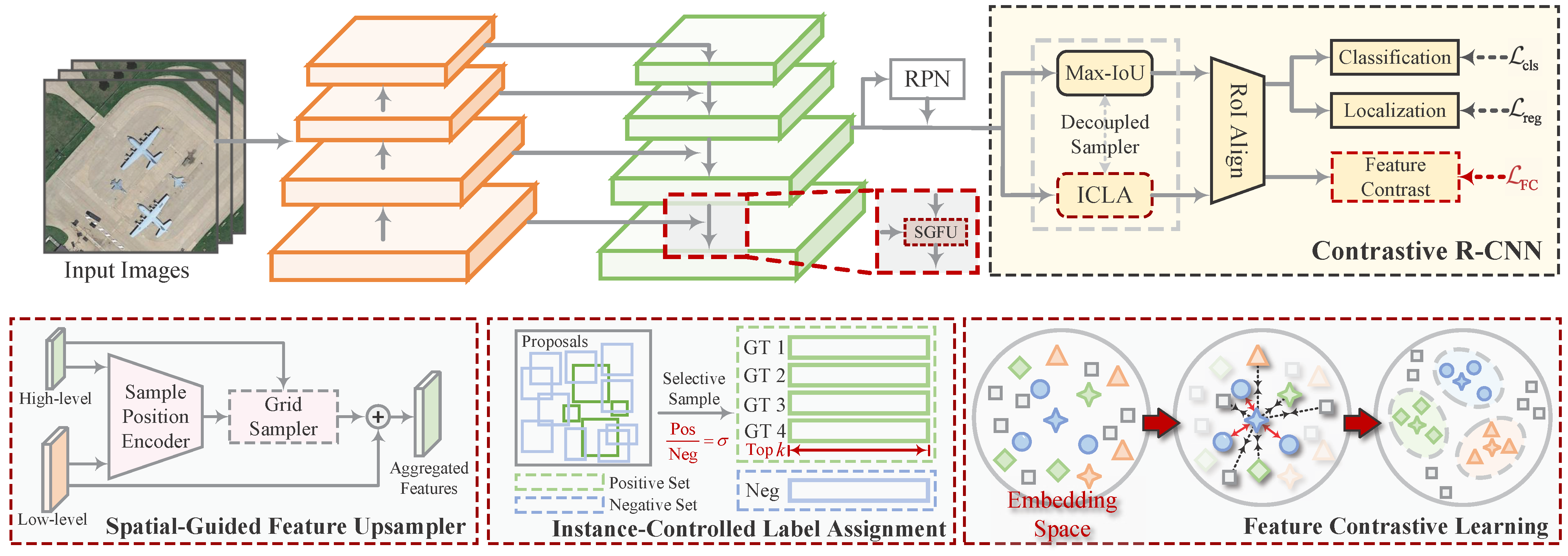
The overall structure of our FCDet is shown in
Figure 3. Our proposed method is built on Faster R-CNN [
37]. Given a remote sensing image, the backbone first performs hierarchical feature extraction. Next, the feature pyramid network (FPN) [
38] aggregates features across different scales. We integrate SGFU into the FPN, replacing the original interpolation method. SGFU dynamically samples spatial positions to enable a learnable upsampling process, ensuring spatial alignment during adjacent feature fusion. Subsequently, the fused features, along with the proposals generated by the RPN, are fed into the contrastive R-CNN. The proposed FCH projects RoI features into an embedding space to measure the distance between samples. To regulate the influence of sample pairs on contrastive feature learning, ICLA selects appropriate positive and negative samples for FCH. Finally, the regression head in the contrastive R-CNN predicts refined object locations, while the classification head outputs category scores. Through iterative training, the model parameters are optimized.
3.1. Spatial-Guided Feature Upsampler
FPN employs a top-down feature aggregation flow, allowing high-level semantic information to be transmitted to lower-level features. This is a crucial discriminative factor, particularly for small weak objects with limited information. However, FPN relies on interpolation to align adjacent features. This fixed-rule approach tends to cause spatial misalignment, where different-level features do not spatially correspond. Inspired by Dysampler [
32], we introduce low-level features rich in spatial information to guide feature upsampling. The sampling positions are dynamically determined by considering the spatial distribution of semantic information.
The full process of the proposed SGFU is illustrated in
Figure 4. Its core concept is to dynamically compute the spatial position for each upsampling point. Unlike linear interpolation, SGFU takes both the higher-level feature
and the lower-level feature
from adjacent levels as input, producing the upsampled feature
as output. First, for the inputs
and
, a 1 × 1 convolution followed by group normalization (GN) is applied to unify the dimensions to
C and normalize the data to enhance robustness. Next, we compute the offset for each sampling point corresponding to an upsampling position by linearly mapping
to
in parallel. Here,
and
represent the coordinates of the offset points, while 2 denotes the offset values in the
x- and
y- directions. For specialized prediction of the offsets for the top-left, top-right, bottom-left, and bottom-right positions, we decouple the prediction into four parallel linear mapping branches. These parallel offsets are then concatenated along the channel dimension and reorganized into an offset matrix
using pixel shuffling. It can be expressed as
where
represents the 1 × 1 convolution, off represents the predicted offset, and Concat represents the concatenation operation.
Although offset prediction introduces flexibility for feature upsampling, relying solely on the position of the sampled features is insufficient to accurately represent the geometric information during feature aggregation. Even after applying offsets, the upsampled features may lack precise spatial correspondence. To address this issue, we incorporate low-level features to guide the prediction of upsampling positions. For feature
, we similarly apply convolution and GN to align its data distribution with that of
. We then linearly project it to
to represent spatial offsets
. A sigmoid function is adopted to constrain the offsets and prevent excessive shifts that could lead to instability. Next, we add
to
to obtain the offset corresponding to each upsampling position. This incorporates the spatial information from the lower-level features, reducing the likelihood of inaccurate pixel interpolation. The computed offsets are added to the grid points to generate the final sampling coordinates, which are subsequently normalized to the range of (−1, 1). Leveraging these coordinates, SGFU performs pixel-wise sampling from
to construct the upsampled feature
. The value of
not only captures the semantic relationships in the image but also incorporates crucial spatial information. This enables it to effectively convey useful information for small, weak objects during feature aggregation. The above process can be expressed as
where
represents the coordinates of the grid points, and
denotes the sampling coordinates.
refers to the grid sampler, whose workflow is illustrated in
Figure 5. Based on the specified positions within the sampling coordinates, the sampler extracts the corresponding pixel values by performing bilinear interpolation on the four nearest pixels, filling the results into the corresponding positions. This process queries the key feature locations and interpolates the fine-grained features. After traversing the entire grid pixel by pixel, the network obtains high-resolution features.
To provide a comprehensive overview of SGFU, we formally summarize the aforementioned pipeline in Algorithm 1. In summary, the proposed upsampler adaptively adjusts sampling positions based on the semantic content and spatial distribution of the input features. This ensures spatial consistency while preserving both feature details and representations. Compared to fixed upsampling methods, SGFU provides precise alignment during feature aggregation.
| Algorithm 1 Spatial-guided feature upsampling (SGFU). |
| Input: Input features , |
| Output: Upsampled features |
- 1:
Feature Normalization: - 2:
▹ 1 × 1 conv + GroupNorm - 3:
- 4:
Offset Prediction: - 5:
for to 4 do ▹ Parallel offset branches - 6:
- 7:
- 8:
Spatial Guidance: - 9:
▹ Constrained to (0, 1) - 10:
Coordinate Computation: - 11:
▹ Normalize to (−1, 1) - 12:
Feature Upsampling: - 13:
▹ Bilinear interpolation - 14:
return
|
3.2. Feature-Contrastive Learning
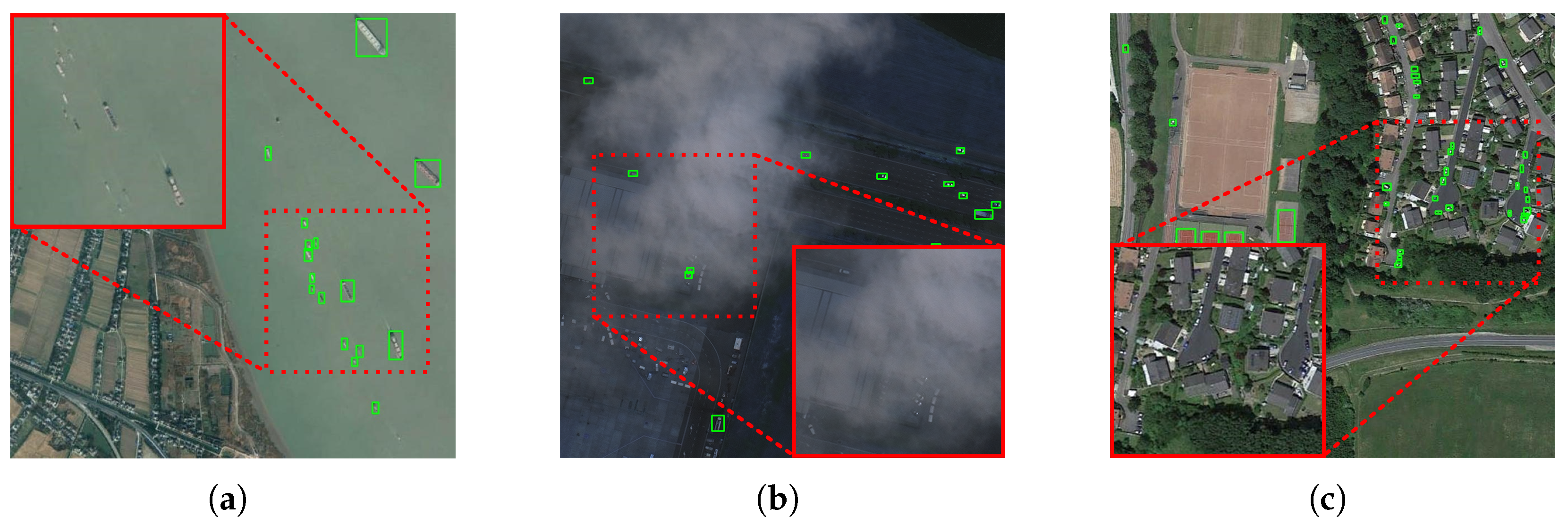
As illustrated in
Figure 1, small and weak objects often exhibit high visual similarity to their surrounding context, making it challenging for the network to extract valuable discriminative information from backgrounds with similar colors. Existing methods [
19,
20,
21] attempt to enhance feature representation by incorporating complex structures or attention mechanisms. In contrast, we aim to strengthen the model’s response to challenging objects using contrastive learning, which allows the network to discover inherent patterns in unlabeled data. By projecting data into the embedding space, contrastive learning brings similar data points closer together while pushing dissimilar points apart. Inspired by this, we leverage contrastive learning to explore the similarity and dissimilarity potentials within the feature space, thereby improving networks to detect weak-response objects.
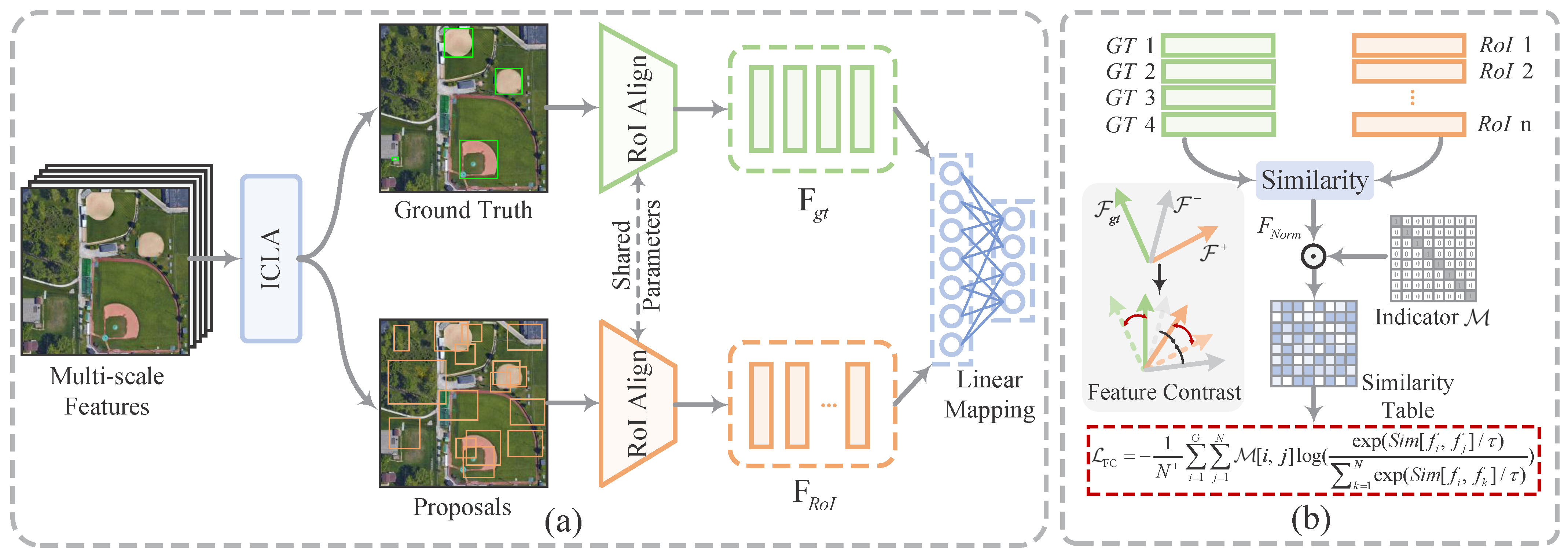
The complete process of FCL is shown in
Figure 6. Specifically, the important concept in contrastive learning is the definition of positive and negative sample pairs, which are used to distinguish between different data. Upon extracting the RoI features, we define anchors as well as positive and negative sample pairs. The network extracts the RoI features from the ground truth as the anchor, denoted as
. For the specified anchor
, the positive samples assigned during label assignment are defined as the positive samples here, marked as
. The positive samples from the remaining ground truth, along with all negative samples, are designated as negative samples relative to
, labeled as
. This can be expressed as
where
is an identifier used to mark samples,
represents the assigned set of positive samples, and
is the RoI feature extracted from the proposal
.
During the RoI feature extraction stage, RPN generates proposals based on the multi-scale feature maps produced by FPN. These proposals are subsequently projected onto their corresponding regions within the feature maps. FCH then utilizes RoI Align with bilinear interpolation to achieve precise feature sampling, producing standardized RoI features with fixed dimensions (
). These extracted features effectively combine fine-grained local patterns with high-level semantic information. After labeling these RoIs, the features are forwarded to the FCH for representation learning.
Figure 3 illustrates the constructed contrastive R-CNN, which integrates the FCH in parallel with the classification and regression heads. The FCH comprises two linear mapping layers that project the input features into a low-dimensional embedding space for distance measurement. Specifically, we define the dimensions of the input RoI features
and
as
and
, respectively, where
N denotes the number of samples and
G denotes the number of ground truths. FCH initially applies global average pooling followed by a flattening operation to transform the dimensions of
and
into
and
, respectively. Subsequently, a linear projection layer reduces their dimensionality to
and
in a channel-wise manner. The compressed embeddings preserve the semantic information from the original features while reducing representation costs. In the embedding space, we utilize cosine similarity to measure the distance between samples, which can be expressed as
where
i and
j are data used to calculate the cosine similarity.
In general, the InfoNCE loss [
39] serves as a fundamental tool in contrastive learning that drives the optimization of similarity between sample data. It enhances the ability of models to aggregate positive samples while increasing the disparity among negative samples. This loss can be expressed as follows:
where
N represents the number of samples,
and
denote the representation vectors of positive samples, and
denotes the representation vector of negative samples;
is the temperature parameter, which adjusts the sensitivity to negative samples. In Equation (
9), the more similar a negative sample is to the anchor, the larger the penalty term generated by
. This loss drives the network to separate sample distances in the embedding space, facilitating data discrimination.
We design a feature contrast loss
that optimizes the aforementioned computations. Specifically, the network first evaluates the cosine similarity between the anchor
and the sample
using Equation (
7). Subsequently, the similarity table is transformed into a normalized probability distribution
through the softmax function, with a temperature coefficient
set to control the sample distribution:
This process effectively assigns attention weights to the samples, highlighting the relative importance of the data. Spatially, positive samples are predominantly extracted from specific structures or local contextual regions of the ground truth. These samples carry significant co-occurrence information that indicates the fundamental attributes of the ground truth. Therefore, in feature measurement, positive samples need particular attention, as they provide valuable guidance for feature learning. By introducing the indicator
, we retain only the positive sample probability scores for each anchor. It is important to note that this approach does not overlook the contribution of negative samples. On the contrary, negative samples corresponding to similar backgrounds are implicitly amplified through the penalty probability density
of
. Finally, we compute the feature contrastive loss to facilitate feature discrimination learning. The overall process can be represented as follows:
where
represents the probability distribution of the samples, and
denotes the number of positive samples.
Our proposed FCL differs from PCLDet in three key aspects: (1) In terms of loss computation, FCL focuses on optimizing the similarity of positive samples while implicitly balancing the influence of negative samples, achieving automatic adjustment between positive and negative contributions; (2) For anchor sample selection, FCL directly utilizes RoI features of real instances, which better captures intra-class variations compared to PCLDet’s use of class prototypes, making it particularly suitable for small, weak object detection; (3) In sample generation, FCL adopts a decoupled ICLA strategy instead of PCLDet’s shared sampler, offering greater flexibility and avoiding interference with other training tasks.
For SWOD, the proposed method guides the network to progressively learn to distinguish and associate features of real samples. The model is capable of capturing and implicitly amplifying subtle feature differences, which is particularly crucial for detecting small, weak objects that closely resemble the background.
3.3. Instance-Controlled Label Assignment
In FCL, positive samples enhance the consistency of representations for the same instance and improve the robustness of the model. Negative samples help prevent feature confusion and reduce interference from similar backgrounds. Therefore, the selection of positive and negative samples is crucial for representation learning. However, existing methods fail to provide the most suitable samples due to the difficulty in controlling sample definitions. To address this, and to explore the potential of contrastive learning in object detection, we propose a simple yet effective label assignment strategy. This method allows manual control over the ratio and number of positive and negative samples according to the network’s requirements.
Specifically, given that the total number of proposals to be sampled is
N and the number of ground truth is
G, the number of positive samples
can be calculated as
where
is a ratio parameter controlling the balance between positive and negative samples. We adopt a simple averaging strategy, treating each ground truth equally. Accordingly, the number of positive samples
k assigned to each ground truth can be calculated as
where
represents the rounding function. Positive samples should have similar semantic representations to the ground truth, as they directly influence the quality of feature contrast. Thus, these samples should be spatially close to the ground truth and have overlapping parts. To achieve this, we use the intersection over union (IoU) metric to determine positive samples. The sampler selects the top
k samples with the highest overlap with the ground truth as positive samples, which can be expressed as
where
represents the set of positive samples for the ground truth
,
denotes the set of candidate samples.


