Abstract
Despite advances in remote sensing object detection, accurately identifying small, weak objects remains challenging. Their limited pixel representation often fails to capture distinctive features, making them susceptible to environmental interference. Current detectors frequently miss these subtle feature variations. To address these challenges, we propose FCDet, a feature contrast-based detector for small, weak objects. Our approach introduces: (1) a spatial-guided feature upsampler (SGFU) that aligns features by adaptive sampling based on spatial distribution, thus achieving fine-grained alignment during feature aggregation; (2) a feature contrast head (FCH) that projects GT and RoI features into an embedding space for discriminative learning; and (3) an instance-controlled label assignment (ICLA) strategy that optimizes sample selection for feature contrastive learning. We conduct comprehensive experiments on challenging datasets, with the proposed method achieving 73.89% mAP on DIOR, 95.04% mAP on NWPU VHR-10, and 26.4% AP on AI-TOD, demonstrating its effectiveness and superior performance.
1. Introduction
Due to interference from factors such as high imaging altitude and the imaging environment, small and weak objects are widely distributed in remote sensing images [1]. These objects typically exhibit characteristics of low signal-to-noise ratio (SNR) and insufficient structural information, resulting in weak feature responses. According to [2], their small scale, low SNR, and influence of complex contexts contribute to the manifestation of weak characteristics. This exponentially increases the difficulty of detecting small and weak objects compared to general objects. However, high-precision small and weak object detection (SWOD) is of great significance across various fields, including agricultural monitoring [3], environmental protection [4], and military reconnaissance [5], among others. Such objects often carry more critical information, and accurate detection can significantly enhance decision-making efficiency and response capabilities [6].
Currently, the performance of most mainstream object detection networks significantly lags when dealing with small and weak objects compared to other objects. This disparity primarily arises from the subtlety of key features, which makes it challenging for these objects to effectively convey their attributes. Figure 1 illustrates several examples of small and weak objects. In Figure 1a, these objects display blurred appearances and details, limited by both the spatial resolution and their inherent characteristics. In Figure 1b, atmospheric obstruction and lighting conditions further obscure the details of the objects, exacerbating their weak attributes. Similarly, in Figure 1c, complex contexts can significantly influence objects, complicating the process of filtering out large amounts of irrelevant information. Consequently, the objects may become overwhelmed by the background. These factors collectively hinder feature expression. From the network perspective, it is difficult for the model to learn inconspicuous features from challenging contexts, resulting in widespread neglect of small and weak objects [7]. From the feature perspective, misalignment during multi-resolution feature aggregation further undermines the representation of key semantic features [8]. Figure 2 visualizes the feature representations at adjacent levels in the feature pyramid network (FPN). It is clear that the interpolated features do not accurately align with the spatial distribution of low-level features. Due to rough interpolation operations, the restored semantic information fails to precisely match the corresponding spatial positions. This not only hinders effective feature aggregation but also introduces additional noise interference, particularly for small and weak objects (see the red dashed box). Therefore, the challenges associated with SWOD persist and necessitate urgent attention and resolution.
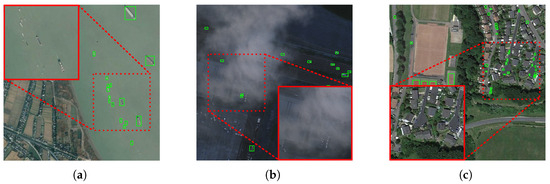
Figure 1.
Some typical attributes that affect small, weak objects: (a) objects with ambiguous appearance and details; (b) objects with low signal-to-noise ratio; (c) objects in complex contexts.
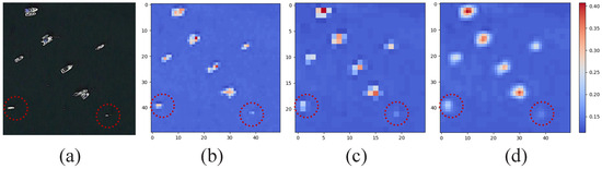
Figure 2.
Demonstration of feature misalignment caused by simple bilinear interpolation during adjacent-level feature aggregation: (a) input images; (b) low-level features; (c) high-level features; (d) interpolated features.
Significant efforts have been dedicated to improving the performance of small and weak objects in image interpretation and analysis. Zhang et al. [9] designed a gated context aggregation module to enhance the feature representation of small and weak objects by aggregating contextual information. FSANet [10] introduced a feature-aware alignment module to mitigate the effects of spatial misalignment on feature fusion and proposed a spatial-aware guidance head that leverages the shapes of small objects to inform predictions. SRNet [11] identified the locations of potential objects using a region search module, restoring the boundary structures and texture features of small objects in camouflage detection. DSNet [12] employed a dual-branch architecture to encode and interact with small object features, utilizing global and mutual constraints to differentiate foreground and background for camouflaged objects. PRNet [13] integrated multi-scale features through a proposed cascaded attention perceptron to locate camouflaged objects, extract contextual information, and aggregate details to refine results further. PBTA [14] utilized a partial break bidirectional feature pyramid network to address scale confusion and semantic loss issues in small pedestrian detection. In moving vehicle detection, SDANet [15] customized a bidirectional Conv-RNN module to align disturbed backgrounds, alleviating the lack of appearance information for small vehicles. However, these studies primarily focus on structurally modifying or adding extra components to enhance the network’s extraction capabilities. They tend to overlook the impact of the inconspicuousness of small and weak object features, as well as how existing networks can improve their learning and discrimination abilities. As a result, these methods still have limitations in detecting weak objects.
In this paper, we aim to enhance the learning capabilities of the network to improve the detection performance of small and weak objects. Specifically, a feature contrast-based detector (FCDet) is developed for SWOD in remote sensing. First, to address the misalignment issues in feature aggregation for small and weak objects, we propose a spatial-guided feature upsampler (SGFU). SGFU follows a learnable upsampling way, where the sampling locations are determined jointly by both high- and low-resolution features. This enables the acquisition of finely aligned semantic features. Second, we construct a contrastive R-CNN network by introducing a feature contrast head (FCH) that operates in parallel with the classification and localization branches. The FCH effectively mitigates background interference by employing feature contrastive learning (FCL) to guide the model in focusing on the differences between small and weak objects and similar backgrounds. Furthermore, the model can learn richer and more discriminative features, providing a better representation of small and weak objects. Finally, to exploit the learning capability of FCH, we propose an instance-controlled label assignment strategy (ICLA). ICLA introduces adjustable ports for positive and negative samples within the contrastive R-CNN network. By modifying the ratio and quantity of samples, the FCH promotes aggregation and uniformity among the contrastive sample pairs, thereby driving the network to effectively learn feature discrimination. To demonstrate the effectiveness of the proposed method, we conduct extensive experiments on three large-scale datasets: DIOR [16], NWPU VHR-10 [17], and AI-TOD [18]. The experimental results indicate that the proposed method achieves superior performance, particularly in SWOD. The main contributions of this paper are summarized as follows:
- A SGFU is proposed to align spatial patterns in feature aggregation by adaptively adjusting the sampling locations based on the learned spatial feature distribution.
- A contrastive learning-based FCH is introduced to guide the network in distinguishing between object features and context. The inconspicuous key features of the objects can be captured, especially for small and weak ones.
- A simple yet effective ICLA strategy is designed to regulate the effects of positive and negative sample pairs on feature learning. Diverse samples can also enhance the feature representation of the objects.
The remaining sections of this article are organized as follows: Section 2 offers a brief review of related work, including small weak object detection, contrastive learning, and feature upsampling. Section 3 provides a detailed description of the proposed FCDet. Experimental results and analysis are presented in Section 4. Section 5 concludes the article.
2. Related Work
2.1. Small Weak Object Detection
Due to the small scale and inconspicuous features, detecting small and weak objects remains a challenge in remote sensing [2]. Currently, several methods have made considerable efforts to improve the discriminability of these objects. TBNet [19] explored important texture patterns and boundary cues to enhance the feature representation of small and weak objects, while also introducing a task-decoupled detection head to address the entanglement of classification and regression tasks. Li et al. [20] proposed a context integration module that develops an RFConv to integrate contextual information from various receptive fields for small and weak objects. Han et al. [21] adopted a context-driven approach, leveraging surrounding information to augment the key features of small and weak objects. Ma et al. [22] introduced a category-aware module that separates features of different categories into distinct channels. This approach effectively reduces interference from inter-class features and background noise. Guo et al. [23] proposed a hierarchical activation method that activates features at different scales to obtain pure features. This method alleviates the interference caused by feature overlap between classes for small objects. However, absorbing cues from external sources may lead to interference, as irrelevant information can further weaken feature representations.
In contrast, we enhance the learning ability of the networks to differentiate object features from highly similar environments through a self-supervised learning strategy. This approach projects the extracted features into an embedding space and employs loss constraints to minimize the distance between relevant features while maximizing the distance between irrelevant features based on their differences. This effectively enhances the discernibility of small and weak objects in complex backgrounds.
2.2. Contrastive Learning
Self-supervised learning [24] is an emerging paradigm that automatically generates labels from the internal attributes of the data to guide model training. It can reduce the reliance on manually annotated labels. As a form of self-supervised learning, contrastive learning has garnered increasing attention and research, gradually expanding into the field of object detection. It aligns similar features in the embedding space by leveraging the information similarity between constructed sample pairs while ensuring a uniform distribution of irrelevant features. Yuan et al. [25] designed a feature imitation branch to enhance the feature representation of small objects and employed contrastive loss for self-supervised training. Liu et al. [26] constructed semantic-level and geometric-level feature relations to eliminate noise interference in the feature pyramid. Lv et al. [27] developed a contrastive detection head for ship detection in SAR images, encoding positive and negative samples into a contrastive feature space for feature learning. PCLDet [28] introduced prototypical contrastive learning for fine-grained object detection. It constructed a prototype bank for each category as an anchor, minimizing the intra-class feature distance while maximizing the inter-class distance to extract discriminative features. Chen et al. [29] proposed a few-shot object detection method based on multi-scale contrastive learning. This method utilizes Siamese structures to process proposals and multi-scale objects and introduces a contrastive multiscale proposal loss to guide multi-scale contrastive learning.
These methods illustrate that contrastive learning can effectively enhance the discriminative ability of objects. To leverage this advantage, we aim to extend it to SWOD. We adopt the features of ground truth as anchors in contrastive learning, assigning the positive RoI features as positive samples while treating the remaining RoI features as negative samples. Through self-supervised iterative training, the representation of weak objects is gradually enhanced.
2.3. Feature Upsample
Feature upsampling is a critical technique for cross-scale feature fusion in object detection. It restores high-resolution feature maps using specific interpolation algorithms, such as nearest neighbor interpolation, bilinear interpolation, and bicubic interpolation. These traditional methods estimate new pixel values based on surrounding ones but are inherently rigid, often leading to unstable results in complex scenes. In contrast, learning-based upsampling methods, like deconvolution (Deconv) [30] and pixel shuffle [31], introduce learnable kernel functions that offer greater flexibility and can overcome the limitations of fixed-rule interpolation techniques. Currently, several methods [32,33,34,35,36] introduce more flexible strategies for feature upsampling. For example, Liu et al. [32] proposed a dynamic point-based sampler that performs lightweight interpolation by searching for the interpolation positions. CARAFE [33] predicts a specific deconvolution kernel for each pixel location, where the predicted kernel incorporates local contextual information to assist in feature reorganization. Mazzini [34] introduced a guided upsampling module that predicts a high-resolution compensation table to guide nearest-neighbor upsampling in semantic segmentation. FADE [35] presents a task-agnostic upsampling operator that combines high- and low-resolution features to generate upsampling kernels, refining the upsampled features through a gated filter. SAPA [36] computes the mutual similarity between encoder and decoder features and transforms the computed scores into upsampling kernel weights.
The mentioned methods have specifically refined upsampling kernels to meet the demands of different tasks better. To achieve spatial alignment for feature aggregation in SWOD, we develop a flexible upsampler SGFU. Inspired by the idea of dynamically predicting sampling positions, our proposed upsampler guides the upsampling process according to the spatial position distribution, which can produce more precise high-resolution features.
3. Proposed Method
The overall structure of our FCDet is shown in Figure 3. Our proposed method is built on Faster R-CNN [37]. Given a remote sensing image, the backbone first performs hierarchical feature extraction. Next, the feature pyramid network (FPN) [38] aggregates features across different scales. We integrate SGFU into the FPN, replacing the original interpolation method. SGFU dynamically samples spatial positions to enable a learnable upsampling process, ensuring spatial alignment during adjacent feature fusion. Subsequently, the fused features, along with the proposals generated by the RPN, are fed into the contrastive R-CNN. The proposed FCH projects RoI features into an embedding space to measure the distance between samples. To regulate the influence of sample pairs on contrastive feature learning, ICLA selects appropriate positive and negative samples for FCH. Finally, the regression head in the contrastive R-CNN predicts refined object locations, while the classification head outputs category scores. Through iterative training, the model parameters are optimized.
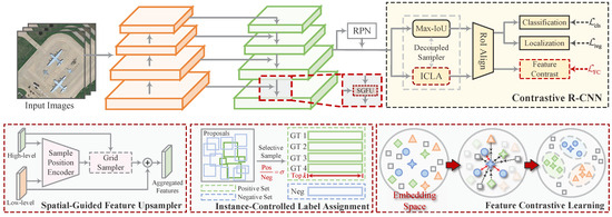
Figure 3.
Overall structure of the proposed FCDet for small weak object detection, including the proposed SGFU, ICLA, and FCL illustrated below.
3.1. Spatial-Guided Feature Upsampler
FPN employs a top-down feature aggregation flow, allowing high-level semantic information to be transmitted to lower-level features. This is a crucial discriminative factor, particularly for small weak objects with limited information. However, FPN relies on interpolation to align adjacent features. This fixed-rule approach tends to cause spatial misalignment, where different-level features do not spatially correspond. Inspired by Dysampler [32], we introduce low-level features rich in spatial information to guide feature upsampling. The sampling positions are dynamically determined by considering the spatial distribution of semantic information.
The full process of the proposed SGFU is illustrated in Figure 4. Its core concept is to dynamically compute the spatial position for each upsampling point. Unlike linear interpolation, SGFU takes both the higher-level feature and the lower-level feature from adjacent levels as input, producing the upsampled feature as output. First, for the inputs and , a 1 × 1 convolution followed by group normalization (GN) is applied to unify the dimensions to C and normalize the data to enhance robustness. Next, we compute the offset for each sampling point corresponding to an upsampling position by linearly mapping to in parallel. Here, and represent the coordinates of the offset points, while 2 denotes the offset values in the x- and y- directions. For specialized prediction of the offsets for the top-left, top-right, bottom-left, and bottom-right positions, we decouple the prediction into four parallel linear mapping branches. These parallel offsets are then concatenated along the channel dimension and reorganized into an offset matrix using pixel shuffling. It can be expressed as
where represents the 1 × 1 convolution, off represents the predicted offset, and Concat represents the concatenation operation.
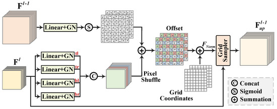
Figure 4.
Processing flow of the proposed SGFU.
Although offset prediction introduces flexibility for feature upsampling, relying solely on the position of the sampled features is insufficient to accurately represent the geometric information during feature aggregation. Even after applying offsets, the upsampled features may lack precise spatial correspondence. To address this issue, we incorporate low-level features to guide the prediction of upsampling positions. For feature , we similarly apply convolution and GN to align its data distribution with that of . We then linearly project it to to represent spatial offsets . A sigmoid function is adopted to constrain the offsets and prevent excessive shifts that could lead to instability. Next, we add to to obtain the offset corresponding to each upsampling position. This incorporates the spatial information from the lower-level features, reducing the likelihood of inaccurate pixel interpolation. The computed offsets are added to the grid points to generate the final sampling coordinates, which are subsequently normalized to the range of (−1, 1). Leveraging these coordinates, SGFU performs pixel-wise sampling from to construct the upsampled feature . The value of not only captures the semantic relationships in the image but also incorporates crucial spatial information. This enables it to effectively convey useful information for small, weak objects during feature aggregation. The above process can be expressed as
where represents the coordinates of the grid points, and denotes the sampling coordinates. refers to the grid sampler, whose workflow is illustrated in Figure 5. Based on the specified positions within the sampling coordinates, the sampler extracts the corresponding pixel values by performing bilinear interpolation on the four nearest pixels, filling the results into the corresponding positions. This process queries the key feature locations and interpolates the fine-grained features. After traversing the entire grid pixel by pixel, the network obtains high-resolution features.
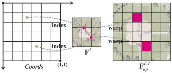
Figure 5.
Demonstration of the grid sampling function. The network progressively samples features from the source features using the input grid (normalized coordinates), interpolates (e.g., bilinearly) at non-integer positions, and obtains flexibly upsampled features .
To provide a comprehensive overview of SGFU, we formally summarize the aforementioned pipeline in Algorithm 1. In summary, the proposed upsampler adaptively adjusts sampling positions based on the semantic content and spatial distribution of the input features. This ensures spatial consistency while preserving both feature details and representations. Compared to fixed upsampling methods, SGFU provides precise alignment during feature aggregation.
| Algorithm 1 Spatial-guided feature upsampling (SGFU). |
| Input: Input features , |
| Output: Upsampled features |
|
3.2. Feature-Contrastive Learning
As illustrated in Figure 1, small and weak objects often exhibit high visual similarity to their surrounding context, making it challenging for the network to extract valuable discriminative information from backgrounds with similar colors. Existing methods [19,20,21] attempt to enhance feature representation by incorporating complex structures or attention mechanisms. In contrast, we aim to strengthen the model’s response to challenging objects using contrastive learning, which allows the network to discover inherent patterns in unlabeled data. By projecting data into the embedding space, contrastive learning brings similar data points closer together while pushing dissimilar points apart. Inspired by this, we leverage contrastive learning to explore the similarity and dissimilarity potentials within the feature space, thereby improving networks to detect weak-response objects.
The complete process of FCL is shown in Figure 6. Specifically, the important concept in contrastive learning is the definition of positive and negative sample pairs, which are used to distinguish between different data. Upon extracting the RoI features, we define anchors as well as positive and negative sample pairs. The network extracts the RoI features from the ground truth as the anchor, denoted as . For the specified anchor , the positive samples assigned during label assignment are defined as the positive samples here, marked as . The positive samples from the remaining ground truth, along with all negative samples, are designated as negative samples relative to , labeled as . This can be expressed as
where is an identifier used to mark samples, represents the assigned set of positive samples, and is the RoI feature extracted from the proposal .
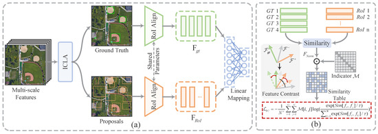
Figure 6.
Detailed demonstration of the proposed feature contrastive learning. (a) Feature space. Following ICLA, the ground truth box and sampled proposals are marked and input into RoI Align to extract RoIs. FCH linearly projects the RoIs into the embedding space for feature representation . (b) Embedding space. The similarity table is calculated among , , and . The feature contrastive loss computes penalties for feature discrimination.
During the RoI feature extraction stage, RPN generates proposals based on the multi-scale feature maps produced by FPN. These proposals are subsequently projected onto their corresponding regions within the feature maps. FCH then utilizes RoI Align with bilinear interpolation to achieve precise feature sampling, producing standardized RoI features with fixed dimensions (). These extracted features effectively combine fine-grained local patterns with high-level semantic information. After labeling these RoIs, the features are forwarded to the FCH for representation learning. Figure 3 illustrates the constructed contrastive R-CNN, which integrates the FCH in parallel with the classification and regression heads. The FCH comprises two linear mapping layers that project the input features into a low-dimensional embedding space for distance measurement. Specifically, we define the dimensions of the input RoI features and as and , respectively, where N denotes the number of samples and G denotes the number of ground truths. FCH initially applies global average pooling followed by a flattening operation to transform the dimensions of and into and , respectively. Subsequently, a linear projection layer reduces their dimensionality to and in a channel-wise manner. The compressed embeddings preserve the semantic information from the original features while reducing representation costs. In the embedding space, we utilize cosine similarity to measure the distance between samples, which can be expressed as
where i and j are data used to calculate the cosine similarity.
In general, the InfoNCE loss [39] serves as a fundamental tool in contrastive learning that drives the optimization of similarity between sample data. It enhances the ability of models to aggregate positive samples while increasing the disparity among negative samples. This loss can be expressed as follows:
where N represents the number of samples, and denote the representation vectors of positive samples, and denotes the representation vector of negative samples; is the temperature parameter, which adjusts the sensitivity to negative samples. In Equation (9), the more similar a negative sample is to the anchor, the larger the penalty term generated by . This loss drives the network to separate sample distances in the embedding space, facilitating data discrimination.
We design a feature contrast loss that optimizes the aforementioned computations. Specifically, the network first evaluates the cosine similarity between the anchor and the sample using Equation (7). Subsequently, the similarity table is transformed into a normalized probability distribution through the softmax function, with a temperature coefficient set to control the sample distribution:
This process effectively assigns attention weights to the samples, highlighting the relative importance of the data. Spatially, positive samples are predominantly extracted from specific structures or local contextual regions of the ground truth. These samples carry significant co-occurrence information that indicates the fundamental attributes of the ground truth. Therefore, in feature measurement, positive samples need particular attention, as they provide valuable guidance for feature learning. By introducing the indicator , we retain only the positive sample probability scores for each anchor. It is important to note that this approach does not overlook the contribution of negative samples. On the contrary, negative samples corresponding to similar backgrounds are implicitly amplified through the penalty probability density of . Finally, we compute the feature contrastive loss to facilitate feature discrimination learning. The overall process can be represented as follows:
where represents the probability distribution of the samples, and denotes the number of positive samples.
Our proposed FCL differs from PCLDet in three key aspects: (1) In terms of loss computation, FCL focuses on optimizing the similarity of positive samples while implicitly balancing the influence of negative samples, achieving automatic adjustment between positive and negative contributions; (2) For anchor sample selection, FCL directly utilizes RoI features of real instances, which better captures intra-class variations compared to PCLDet’s use of class prototypes, making it particularly suitable for small, weak object detection; (3) In sample generation, FCL adopts a decoupled ICLA strategy instead of PCLDet’s shared sampler, offering greater flexibility and avoiding interference with other training tasks.
For SWOD, the proposed method guides the network to progressively learn to distinguish and associate features of real samples. The model is capable of capturing and implicitly amplifying subtle feature differences, which is particularly crucial for detecting small, weak objects that closely resemble the background.
3.3. Instance-Controlled Label Assignment
In FCL, positive samples enhance the consistency of representations for the same instance and improve the robustness of the model. Negative samples help prevent feature confusion and reduce interference from similar backgrounds. Therefore, the selection of positive and negative samples is crucial for representation learning. However, existing methods fail to provide the most suitable samples due to the difficulty in controlling sample definitions. To address this, and to explore the potential of contrastive learning in object detection, we propose a simple yet effective label assignment strategy. This method allows manual control over the ratio and number of positive and negative samples according to the network’s requirements.
Specifically, given that the total number of proposals to be sampled is N and the number of ground truth is G, the number of positive samples can be calculated as
where is a ratio parameter controlling the balance between positive and negative samples. We adopt a simple averaging strategy, treating each ground truth equally. Accordingly, the number of positive samples k assigned to each ground truth can be calculated as
where represents the rounding function. Positive samples should have similar semantic representations to the ground truth, as they directly influence the quality of feature contrast. Thus, these samples should be spatially close to the ground truth and have overlapping parts. To achieve this, we use the intersection over union (IoU) metric to determine positive samples. The sampler selects the top k samples with the highest overlap with the ground truth as positive samples, which can be expressed as
where represents the set of positive samples for the ground truth , denotes the set of candidate samples.
3.4. Loss Function
The overall loss of the network mainly includes four parts, which can be defined as
where represents the loss of the first-stage detection network (RPN), while , , and correspond to the classification loss, regression loss, and feature contrast loss of the second-stage network (contrastive R-CNN), respectively. The expressions , , and are the balancing coefficients for each component. We empirically set , , and . Unless otherwise specified, this configuration will be consistently used in all subsequent experiments. The values of and are set the same as in Faster R-CNN; employs Balanced L1 loss as proposed by [40], which is an optimized version of Smooth L1 loss. The core idea is to enhance the regression gradients of easily classified samples. This approach allows the network to achieve a balanced optimization of classification and localization tasks during the training phase. Balanced L1 loss can be defined as
where the parameters , b, and adjust the regression gradients to achieve a more balanced training process. The relationship can be expressed as follows:
We set , , and following the official settings in [40].
4. Experiments
4.1. Datasets
(1) DIOR is a publicly available large-scale dataset for object detection in remote sensing images. It contains 23,463 optical remote sensing images with a uniform size of 800 × 800, carrying 192,472 axis-aligned annotations. The images exhibit varying resolutions, ranging from 0.5 m to 30 m, to simulate complex remote sensing scenarios. This dataset covers 20 categories: airplane (C1), airport (C2), baseball field (C3), basketball court (C4), bridge (C5), chimney (C6), dam (C7), expressway service area (C8), expressway toll station (C9), golf course (C10), ground track field (C11), harbor (C12), overpass (C13), ship (C14), stadium (C15), storage tank (C16), tennis court (C17), train station (C18), vehicle (C19), and windmill (C20). In our experiments, 11,725 images from the Trainval set were utilized for training, while 11,738 images from the Test set were employed for performance evaluation.
(2) NWPU VHR-10 is a high-resolution remote sensing image object detection dataset released by Northwestern Polytechnical University, China. It comprises 650 remote sensing images with spatial resolutions ranging from 0.5 m to 2 m. The dataset includes 10 categories: airplane (AI), ship (SH), storage tank (ST), baseball field (BF), tennis court (TC), basketball court (BC), ground track field (GTF), harbor (HB), bridge (BR), and vehicle (VE). In the latest version, the dataset is partitioned into 1172 images, each with dimensions of 400 × 400 pixels. It specifies a Trainval set consisting of 879 images and a Test set comprising 293 images, with a ratio of 0.75:0.25.
(3) AI-TOD is a large-scale remote sensing dataset specifically collected for small object detection tasks that carries a large number of tiny objects. This dataset contains 28,036 images and 700,621 instances. It includes eight object categories: airplane (AI), ship (SH), person (PE), bridge (BR), swimming pool (SP), windmill (WM), storage tank (ST), and vehicle (VE). The average size of the objects is only 12.7 pixels, located within complex remote sensing environments, such as ocean surfaces, ports, parking lots, streets, and deserts. All images are uniformly sized at 800 × 800 pixels. We utilize the designated Trainval set (14,018 images) for model training and the Test set (14,018 images) for performance evaluation.
4.2. Evaluation Metrics
For the DIOR and NWPU VHR-10 datasets, we adopt the MS COCO benchmark. By setting the IoU threshold to 0.5, we determine true positive (TP), false positive (FP), true negative (TN), and false negative (FN), which are then used to calculate precision (Pr) and recall (R):
The average precision (AP) is a comprehensive metric that allows for the evaluation of precision and recall for a single category of objects. To evaluate the overall performance of the model across different categories, the mean average precision (mAP) is adopted, which is calculated by averaging the AP of all categories. It can be defined as
In the ablation experiments, , , and are employed to evaluate the detection performance on small (0–32 pixels), medium (32–96 pixels), and large (>96 pixels) scale objects, respectively. These metrics facilitate the analysis of performance variations across different object scales.
For the AI-TOD dataset, due to the specific distribution of sizes, more refined metrics have been introduced for performance evaluation. Specifically, following the MS COCO benchmark, (IoU threshold = 0.5) and (IoU threshold = 0.75) are used to assess overall performance. AP is defined as the average from to , with an IoU interval of 0.05. To more accurately evaluate small objects, we further divide objects (0–32 pixels) into very tiny (0–8 pixels), tiny (8–16 pixels), and small scale (16–32 pixels) objects, using , , and for targeted performance evaluation.
To evaluate detection efficiency, the number of parameters (Param), floating point operations (FLOPs), and frames per second (FPS) are also compared in the ablation experiments.
4.3. Implement Details
We build the experimental environment on two RTX 3090 hardware platforms, each with 24 GB of memory, running the Ubuntu 20.01 system. All experiments are conducted using PyTorch 1.13 and the MMDetection toolbox [41]. AdamW is selected as the optimizer, with the input image size specified as 800 × 800 pixels. For the DIOR dataset, the number of epochs is set to 12, with an initial learning rate of 0.0001 and weight decay of 0.0001. The learning rate is reduced by a factor of 10 at the 8th and 11th epochs. For the NWPU VHR-10 and AI-TOD datasets, the number of epochs is set to 36, with learning rate decay occurring at the 24th and 33rd epochs. Our method is built on Faster R-CNN, utilizing ResNet-50 as the backbone, loaded with parameters pre-trained on ImageNet. The confidence score is set to 0.05.
4.4. Ablation Study
To comprehensively evaluate the effectiveness of each proposed component and its compatibility, we conduct extensive ablation experiments on the DIOR dataset. The experimental results are shown in Table 1. The baseline is Faster R-CNN with FPN. In all ablation experiments, the parameter settings are kept consistent to ensure a fair performance comparison. The baseline achieves 70.19% mAP on the DIOR dataset, and all ablation results are compared against this baseline to explore the effectiveness of the proposed method.

Table 1.
Ablation results (%) of the three proposed components on the DIOR dataset.
4.4.1. Effect of SGFU
In Table 1, the proposed SGFU achieves 71.88% mAP, an improvement of 1.69% compared to the baseline. It can be attributed to the network mitigating feature misalignment caused by interpolation during feature aggregation and restoring more refined features. During feature upsampling, SGFU considers the spatial positions of high-resolution features and adaptively computes the sampling locations for each pixel based on the semantic distribution of the features to be sampled. In detailed metrics, SGFU comprehensively improves the detection accuracy of objects across various scales. Specifically, it increases the from 25.16% to 27.20% (↑2.04%), the from 58.13% to 59.09% (↑0.96%), and the from 87.55% to 88.78% (↑1.23%). Notably, the most significant gains are observed for small objects. This is likely due to feature misalignment severely disrupting the feature representation of small objects during the fusion process, which further degrades their performance. The proposed SGFU dynamically determines the content for upsampling, which alleviates the blurring of information for small objects, as reflected in the performance. We visualize the feature heatmaps to intuitively demonstrate the effect of SGFU. In Figure 7a, the network does not activate the object region. After applying SGFU, the small object features are emphasized and spatially align with the object in Figure 7c. It is important to note that SGFU is a lightweight module with high-performance gains. It introduces only 0.01 M Params and 0.24 G FLOPs, which is negligible.
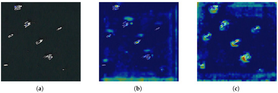
Figure 7.
Visualization comparison of feature heatmaps: (a) input image; (b) feature heatmap output by the baseline; (c) feature heatmap output by the SGFU.
We also compare various upsampling methods, including interpolation-based techniques such as nearest neighbor interpolation and bilinear interpolation, as well as learning-based approaches such as DeConv [30], Pixel Shuffle [31], Dysample [32], and CARAFE [33], to demonstrate the advantages of SGFU. The experimental results are presented in Table 2. Nearest neighbor and bilinear both calculate pixel values based on fixed linear rules. This approach lacks flexibility and fails to account for complex scenes. Numerically, both methods achieve similar performance, with nearest neighbor reaching 70.22% mAP and bilinear reaching 70.18% mAP. In contrast, the learnable Deconv can recover more details through training, which demonstrates satisfactory performance in image super-resolution tasks. However, deconvolution lacks prior guidance and is prone to introducing noise and artifacts during upsampling. As shown in Table 2, Deconv leads to a decrease of 0.90% mAP, with the dropping from 24.38% to 22.79% (↓1.59%). Similarly, Pixel Shuffle improves resolution by integrating and rearranging pixels and is commonly used in image generation tasks. However, this method is not well-suited for the current task, resulting in a decline of 1.16% mAP. This may be due to information loss when processing high-dimensional features. The above two learnable methods introduce learnable kernels, which increases computational complexity. Dysample is a flexible upsampler that employs dynamic interpolation. However, it neglects the issue of feature alignment and does not consider the spatial distribution of high-resolution features. CARAFE introduces contextual information during feature upsampling, which is beneficial for object detection tasks. This is also reflected in performance, with an increase of 0.97% mAP. The proposed SGFU achieves the most significant performance improvement while introducing only negligible parameters and computational burden, thus demonstrating the effectiveness of our method.
Table 2.
Comparison of various feature upsampling methods on the DIOR dataset.
4.4.2. Effect of FCL
To investigate the effectiveness of the proposed FCL for SWOD, we conduct ablation experiments, as shown in Table 1. When the FCH is incorporated into the detection head for feature learning, the baseline improves by 1.57%, achieving 71.76% mAP. Furthermore, when both the FCL and SGFU are employed concurrently, the baseline exhibits an additional improvement of 3.32%, reaching 73.51% mAP. These results demonstrate that the proposed FCL can effectively constrain the network to learn the similarities and differences between sample features, thereby contributing to the overall performance gain. Notably, the FCL and SGFU are fully compatible, each alleviating the challenges associated with small objects in different aspects and promoting accurate recognition of small objects. This is evidenced by a significant increase in the by 5.98%. It is worth noting that FCL introduces only a minimal number of learning parameters, resulting in a negligible impact on memory cost.
The temperature coefficient controls the discriminative ability for sample distribution in the embedding space. A large coefficient results in a lack of bias when learning negative samples. Conversely, a small coefficient increases the penalty for negative samples, leading the model to focus more on difficult ones. The parameter regulates the scale of the feature contrastive loss, indicating the importance of network learning. Since and jointly influence feature learning, we investigate their combined effects on detection performance. The experimental results are shown in Table 3. When and , FCDet achieves the best performance at 73.89% mAP. At this point, the network produces the most effective supervisory signal, which facilitates learning the representation relationship of sample features.
Table 3.
Comparison of and Values with corresponding mAP, , , and results.
We visualize the training loss of FCDet in Figure 8. It is shown that when and , FCL effectively integrates with other tasks for multi-task learning without adversely affecting their performance. The total loss , regression loss , and classification loss remain optimized throughout the training process. At the same time, decreases rapidly during the initial training stages and gradually stabilizes. This indicates that the network successfully learns the relationships between features in the sample space, facilitating effective feature differentiation.
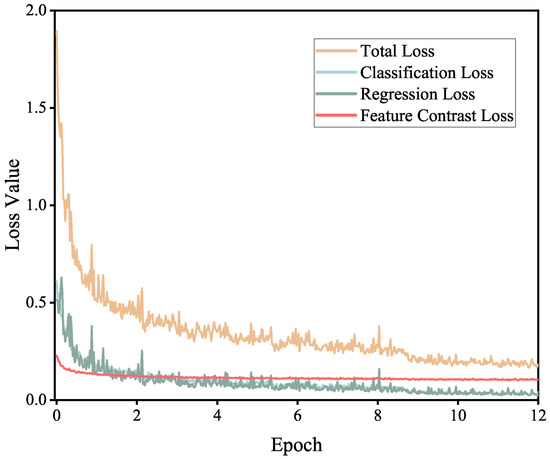
Figure 8.
Visualization of training loss over iterations.
4.4.3. Effect of ICLA
ICLA facilitates sample learning within FCL by enabling precise control over the quantity and ratio of positive and negative samples. It can provide FCH with optimally learnable data. Integrating ICLA into FCL leads to further performance improvements. As shown in Table 1, ICLA improves the mAP from 71.76% to 71.92% when paired solely with FCL, with an gain of 1.67%. This demonstrates that by regulating the sampling of positive and negative samples, the model learns richer feature representations. It enhances the ability of FCDet to differentiate similar features, particularly for small, weak objects. When ICLA is deployed alongside SGFU and FCL, the mAP rises from 73.51% to 73.89% (↑0.38%), with an additional improvement of 0.85%. This indicates that the three proposed components are complementary and provide notable performance gains for small object detection. Furthermore, ICLA introduces no additional parameters and does not affect inference speed.
In contrastive learning, the ratio and quantity of positive and negative samples play a crucial role in model training. Typically, the ratio dictates the learning bias. An overabundance of positive samples may lead the model to overemphasize subtle differences among similar data. At this point, the differences in data between classes will be ignored, leading to a decrease in generalization. Conversely, too many negative samples can also overwhelm the learning signals from related data. Sample quantity, in turn, affects the diversity of feature representations. When sample quantity is too high, the model may struggle to adequately learn the relationships and distinctions among representations, while too few samples can lead to overfitting. Thus, a balance in sample quantity and ratio is essential. To explore the influence of sample configurations on the current task, we conduct comprehensive experiments to uncover the underlying patterns. The experimental results are shown in Table 4 and Table 5. When N = 128 and = 0.1, the model achieves optimal performance on both the DIOR and NWPU VHR-10 datasets. This is likely because the current sample size and ratio yield a balanced contribution from positive and negative samples, preventing the network from overfitting to either type. FCL is capable of both clustering similar samples and separating dissimilar ones, thereby forming a well-structured feature space that enhances the model’s discriminability and robustness. At the same time, ICLA encourages the FCDet to discern correlated features, allowing the network to better learn features that distinguish from background noise, especially for small, weak objects. Adjustments in sample quantity and ratio—whether increased or decreased—correspondingly impact detection performance, further validating the above hypothesis.
Table 4.
Comparison of N and values with corresponding mAP, , , and results on DIOR.
Table 5.
Comparison of N and values with corresponding mAP, , , and results on NWPU VHR-10.
4.5. Comparing State-of-the-Art Methods
4.5.1. Results on DIOR
To demonstrate the advantages of FCDet, we compare several state-of-the-art methods on the DIOR dataset. The experimental results are presented in Table 6. Our FCDet achieves the best performance, with 73.9% mAP. This improvement is attributed to the proposed SGFU, which provides more refined upsampled features and mitigates feature blurring during feature aggregation. FCL enhances the network’s capacity to differentiate among various instances, especially in data that exhibit inter-class similarity and intra-class diversity. Notably, TBNet [19] explores texture and boundary features for small, weak objects. Libra-SOD [42] employs a specialized balanced label assignment strategy for small objects. RingMo-Lite [43] introduces a hybrid CNN–Transformer architecture for interleaving high- and low-frequency feature extraction. All these methods demonstrate competitive performance. However, FCDet achieves improvements of 4.5% to 0.2% over these competitors, which fully validates the effectiveness of the proposed method. Additionally, FCDet achieves 76.5% mAP when Swin-tiny is selected as the extractor. The Transformer can capture more comprehensive global representations, thereby enriching the discernible features for detection tasks. Some representative detection results are visualized in Figure 9. It is evident that FCDet effectively identifies most objects, including visually weak vehicles, ships, and bridges. It also successfully detects objects that closely resemble their environments, such as windmills, golf courses, and baseball fields. These results clearly demonstrate the effectiveness of the proposed method.
Table 6.
The mAP results (%) on DIOR. The best results are marked in bold.
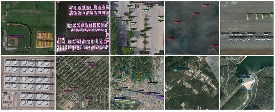
Figure 9.
Some representative small, weak object detection results on the DIOR dataset.
We also compare the efficiency metrics with various methods, as shown in Figure 10. The proposed FCDet maintains high computational efficiency through three key design principles: (1) SGFU employs a lightweight upsampling architecture, (2) FCH introduces minimal parameter overhead (0.02 M parameters), and (3) ICLA only operates during the training stage without inference cost. Compared to the baseline, our method improves mAP by 3.7% at a cost of just 3 FPS. Thus, the proposed method remains competitive regarding parameters and inference speed while maintaining high accuracy.
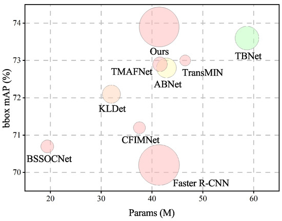
Figure 10.
Comparison of detection performance (mAP), parameters (Params), and inference speed (FPS) of various methods on the DIOR dataset. The size of the circles indicates the inference speed.
4.5.2. Results on NWPU VHR-10
We compare several competitive methods on the NWPU VHR-10 dataset, with the experimental results shown in Table 7. FCDet achieves the best performance, recording 75.04% mAP. Compared to the competitors, our method demonstrates an advantage ranging from 6.74% to 0.25%. This highlights the effectiveness and superiority of FCDet. However, in terms of category-wise performance, FCDet does not exhibit a significant advantage. Except for Airplane and Ground Track Field, the network does not achieve optimal results in other categories. A possible contributing factor is the limited amount of data, which may constrain the learning capacity of FCL. Consequently, the network does not achieve the expected benefits in data fitting.
Table 7.
Comparison of different methods on the NWPU VHR-10 dataset. The best results are marked in bold.
4.5.3. Results on AI-TOD
We conduct comparative experiments on AI-TOD against several of the latest methods, as shown in Table 8. FCDet achieves the best results with 26.4% AP, 57.3% , and 19.9% , which outperforms the competitors by a large margin. Notably, our method achieves 14% , improving performance by 4.6% compared to TBNet [19]. At this scale, the objects often appear weak in appearance, making it difficult to express detailed information. As a result, most detectors perform poorly. However, FCDet demonstrates the capability to recognize discriminative features in complex scenes and remains competitive. In addition, the proposed method achieves 27.2% and 29.5% , also leading in performance. However, it slightly sacrifices performance for large-scale objects due to its extra attention to small, weak objects, which is also reflected in . Moreover, FCDet achieves the best performance in six out of eight categories. Specifically, it obtains 30.0% on Airplane, 59.1% on Ship, 11.5% on Person, 19.3% on Bridge, 20.3% on Swimming Pool, and 26.4% on Vehicle. When adopting Swin-tiny as the extractor, the proposed method further improves the AP to 27.4%. Compared to competitors equipped with the same Swin-tiny, FCDet maintains its lead. We compare the detection results of Faster R-CNN [37], FCOS [58], RetinaNet [59], and TBNet [19] for a visual comparison. In Figure 11, Faster R-CNN and FCOS exhibit significant missed detections due to interference from complex contexts. While RetinaNet recalls some small objects, it still produces several misclassifications on data similar to the objects. TBNet also misclassifies many objects due to their feature similarity. The proposed FCDet effectively distinguishes objects from complex environments via contrastive learning, resulting in satisfactory results.
Table 8.
Comparison of different methods on the AI-TOD dataset. The best results are marked in bold.
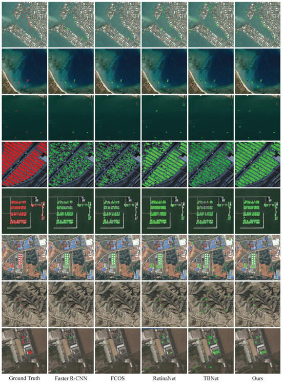
Figure 11.
Comparison of prediction results of various methods on the AI-TOD dataset.
4.6. Discussion
Although FCDet has achieved satisfactory performance, it still has limitations worth discussing. FCL implementation operates exclusively on assigned positive samples, which may induce feature embedding ambiguities when processing visually similar instances within the same category. This design constraint can potentially generate conflicting learning signals for semantically similar features, thereby degrading model discriminability.
In terms of real-time performance, although our two-stage FCDet architecture achieves 40 FPS on modern GPU hardware, its practical deployment faces significant challenges. The computationally intensive nature of both the feature extraction pipeline and anchor prediction mechanisms imposes substantial constraints on real-time performance, particularly for edge devices with limited resources. This computational bottleneck currently restricts the framework’s applicability in mobile and embedded deployment scenarios.
To address these issues, future research will focus on exploring lightweight network architecture designs and incorporating techniques such as model compression and parameter pruning to significantly reduce model complexity. Additionally, we will optimize operator implementations specifically for edge computing devices, aiming to enhance the method’s applicability in resource-constrained scenarios.
5. Conclusions
In this article, we propose FCDet for small, weak object detection in remote sensing. FCDet introduces three key components: SGFU, FCL, and ICLA, to address the challenges associated with small, weak objects. Specifically, SGFU presents a learnable upsampling strategy that adaptively adjusts sampling positions by incorporating spatial prior. The refined features facilitate semantic alignment during feature aggregation. FCL drives the network to learn the relationships among sample feature representations in the embedding space. This enhances its discriminative ability in exploring similar data, particularly for obscure weak objects. We also design a decoupled ICLA strategy to provide richer and more suitable representations for the embedding space. The proposed method demonstrates its effectiveness across three large-scale datasets, especially for small, weak objects.
However, due to limitations in sample annotation, FCDet struggles to perform effective contrastive learning for same-category objects with similar visual appearances. In future work, we will focus on the feasibility of applying contrastive learning to within-class data to mine homogeneous information for weak small objects.
Author Contributions
Conceptualization, Z.L.; methodology, Z.L.; software, X.H.; validation, J.Q.; formal analysis, Z.L.; investigation, Y.W.; resources, Y.W.; data curation, D.X.; writing—original draft preparation, Z.L.; writing—review and editing, Z.L.; visualization, T.Z.; supervision, Y.W.; project administration, Y.W.; funding acquisition, D.X. All authors have read and agreed to the published version of the manuscript.
Funding
This research was funded by the Science and Technology Development Plan Project of Jilin Province grant number 20240101057JC.
Data Availability Statement
The AI-TOD dataset are available from the website https://github.com/Chasel-Tsui/mmdet-aitod.
Acknowledgments
The authors thank the editors and reviewers for their hard work.
Conflicts of Interest
The authors declare no conflicts of interest.
References
- Li, Z.; Wang, Y.; Zhang, N.; Zhang, Y.; Zhao, Z.; Xu, D.; Ben, G.; Gao, Y. Deep Learning-Based Object Detection Techniques for Remote Sensing Images: A Survey. Remote Sens. 2022, 14, 2385. [Google Scholar] [CrossRef]
- Han, W.; Chen, J.; Wang, L.; Feng, R.; Li, F.; Wu, L.; Tian, T.; Yan, J. Methods for Small, Weak Object Detection in Optical High-Resolution Remote Sensing Images: A survey of advances and challenges. IEEE Geosci. Remote Sens. Mag. 2021, 9, 8–34. [Google Scholar] [CrossRef]
- Lin, Z.; He, Z.; Wang, X.; Liang, H.; Su, W.; Tan, J.; Xie, S. Cross-Scale Hybrid Gaussian Attention Network for Object Detection in Remote Sensing Images. IEEE Geosci. Remote Sens. Lett. 2024, 21, 3002305. [Google Scholar] [CrossRef]
- Dong, S.; Wang, L.; Du, B.; Meng, X. ChangeCLIP: Remote sensing change detection with multimodal vision-language representation learning. ISPRS J. Photogramm. Remote Sens. 2024, 208, 53–69. [Google Scholar] [CrossRef]
- Pang, B.; Liu, Y.N. PRO-SSRGAN: Stable super-resolution generative adversarial network based on parameter reconstructive optimization on Gaofen-5 remote-sensing images. Int. J. Remote Sens. 2024, 45, 3022–3053. [Google Scholar] [CrossRef]
- Lin, Q.; Zhao, J.; Fu, G.; Yuan, Z. CRPN-SFNet: A High-Performance Object Detector on Large-Scale Remote Sensing Images. IEEE Trans. Neural Netw. Learn. Syst. 2022, 33, 416–429. [Google Scholar] [CrossRef] [PubMed]
- Li, Z.; Wang, Y.; Feng, H.; Chen, C.; Xu, D.; Zhao, T.; Gao, Y.; Zhao, Z. Local to Global: A Sparse Transformer-Based Small Object Detector for Remote Sensing Images. IEEE Trans. Geosci. Remote Sens. 2025, 63, 5606516. [Google Scholar] [CrossRef]
- Chen, S.; Zhao, J.; Zhou, Y.; Wang, H.; Yao, R.; Zhang, L.; Xue, Y. Info-FPN: An Informative Feature Pyramid Network for object detection in remote sensing images. Expert Syst. Appl. 2023, 214, 119132. [Google Scholar] [CrossRef]
- Zhang, T.; Zhang, X.; Zhu, X.; Wang, G.; Han, X.; Tang, X.; Jiao, L. Multistage Enhancement Network for Tiny Object Detection in Remote Sensing Images. IEEE Trans. Geosci. Remote Sens. 2024, 62, 5606516. [Google Scholar] [CrossRef]
- Wu, J.; Pan, Z.; Lei, B.; Hu, Y. FSANet: Feature-and-Spatial-Aligned Network for Tiny Object Detection in Remote Sensing Images. IEEE Trans. Geosci. Remote Sens. 2022, 60, 5630717. [Google Scholar] [CrossRef]
- Liu, G.; Wu, W. Search and recovery network for camouflaged object detection. Image Vis. Comput. 2024, 151, 105247. [Google Scholar] [CrossRef]
- Yang, H.; Zhu, Y.; Sun, K.; Ding, H.; Lin, X. Camouflaged Object Detection via Dual-branch Fusion and Dual Self-similarity constraints. Pattern Recogn. 2025, 157, 110895. [Google Scholar] [CrossRef]
- Hu, X.; Zhang, X.; Wang, F.; Sun, J.; Sun, F. Efficient Camouflaged Object Detection Network Based on Global Localization Perception and Local Guidance Refinement. IEEE Trans. Circuits Syst. Video Technol. 2024, 34, 5452–5465. [Google Scholar] [CrossRef]
- Sha, X.; Guo, Z.; Guan, Z.; Li, W.; Wang, S.; Zhao, Y. PBTA: Partial Break Triplet Attention Model for Small Pedestrian Detection Based on Vehicle Camera Sensors. IEEE Sens. J. 2024, 24, 21628–21640. [Google Scholar] [CrossRef]
- Feng, J.; Liang, Y.; Zhang, X.; Zhang, J.; Jiao, L. SDANet: Semantic-Embedded Density Adaptive Network for Moving Vehicle Detection in Satellite Videos. IEEE Trans. Image Process. 2023, 32, 1788–1801. [Google Scholar] [CrossRef] [PubMed]
- Li, K.; Wan, G.; Cheng, G.; Meng, L.; Han, J. Object detection in optical remote sensing images: A survey and a new benchmark. ISPRS J. Photogramm. Remote Sens. 2020, 159, 296–307. [Google Scholar] [CrossRef]
- Cheng, G.; Han, J.; Zhou, P.; Guo, L. Multi-class geospatial object detection and geographic image classification based on collection of part detectors. ISPRS J. Photogramm. Remote Sens. 2014, 98, 119–132. [Google Scholar] [CrossRef]
- Wang, J.; Yang, W.; Guo, H.; Zhang, R.; Xia, G.S. Tiny Object Detection in Aerial Images. In Proceedings of the 2020 25th International Conference on Pattern Recognition (ICPR 2021), Milan, Italy, 10–15 January 2021; pp. 3791–3798. [Google Scholar] [CrossRef]
- Li, Z.; Wang, Y.; Xu, D.; Gao, Y.; Zhao, T. TBNet: A texture and boundary-aware network for small weak object detection in remote-sensing imagery. Pattern Recogn. 2025, 158, 110976. [Google Scholar] [CrossRef]
- Li, Z.; Wang, Y.; Zhang, Y.; Gao, Y.; Zhao, Z.; Feng, H.; Zhao, T. Context Feature Integration and Balanced Sampling Strategy for Small Weak Object Detection in Remote Sensing Imagery. IEEE Geosci. Remote Sens. Lett. 2024, 21, 6009105. [Google Scholar] [CrossRef]
- Han, W.; Li, J.; Wang, S.; Wang, Y.; Yan, J.; Fan, R.; Zhang, X.; Wang, L. A context-scale-aware detector and a new benchmark for remote sensing small weak object detection in unmanned aerial vehicle images. Int. J. Appl. Earth Obs. 2022, 112, 102966. [Google Scholar] [CrossRef]
- Ma, W.; Wu, Y.; Zhu, H.; Zhao, W.; Wu, Y.; Hou, B.; Jiao, L. Adaptive Feature Separation Network for Remote Sensing Object Detection. IEEE Trans. Geosci. Remote Sens. 2024, 62, 5639717. [Google Scholar] [CrossRef]
- Guo, G.; Chen, P.; Yu, X.; Han, Z.; Ye, Q.; Gao, S. Save the Tiny, Save the All: Hierarchical Activation Network for Tiny Object Detection. IEEE Trans. Circuits Syst. Video Technol. 2024, 34, 221–234. [Google Scholar] [CrossRef]
- Xie, E.; Ding, J.; Wang, W.; Zhan, X.; Xu, H.; Sun, P.; Li, Z.; Luo, P. DetCo: Unsupervised Contrastive Learning for Object Detection. In Proceedings of the 2021 IEEE/CVF International Conference on Computer Vision (ICCV 2021), Montreal, QC, Canada, 10–17 October 2021; pp. 8372–8381. [Google Scholar] [CrossRef]
- Yuan, X.; Cheng, G.; Yan, K.; Zeng, Q.; Han, J. Small Object Detection via Coarse-to-fine Proposal Generation and Imitation Learning. In Proceedings of the 2023 IEEE/CVF International Conference on Computer Vision (ICCV 2023), Paris, France, 2–3 October 2023; pp. 6294–6304. [Google Scholar] [CrossRef]
- Liu, H.I.; Tseng, Y.W.; Chang, K.C.; Wang, P.J.; Shuai, H.H.; Cheng, W.H. A DeNoising FPN With Transformer R-CNN for Tiny Object Detection. IEEE Trans. Geosci. Remote Sens. 2024, 62, 4704415. [Google Scholar] [CrossRef]
- Lv, Y.; Li, M.; He, Y. An Effective Instance-Level Contrastive Training Strategy for Ship Detection in SAR Images. IEEE Geosci. Remote Sens. Lett. 2023, 20, 4007505. [Google Scholar] [CrossRef]
- Ouyang, L.; Guo, G.; Fang, L.; Ghamisi, P.; Yue, J. PCLDet: Prototypical Contrastive Learning for Fine-Grained Object Detection in Remote Sensing Images. IEEE Trans. Geosci. Remote Sens. 2023, 61, 5613911. [Google Scholar] [CrossRef]
- Chen, J.; Qin, D.; Hou, D.; Zhang, J.; Deng, M.; Sun, G. Multiscale Object Contrastive Learning-Derived Few-Shot Object Detection in VHR Imagery. IEEE Trans. Geosci. Remote Sens. 2022, 60, 5635615. [Google Scholar] [CrossRef]
- Zeiler, M.D.; Taylor, G.W.; Fergus, R. Adaptive deconvolutional networks for mid and high level feature learning. In Proceedings of the 2011 International Conference on Computer Vision, Barcelona, Spain, 6–11 November 2011; pp. 2018–2025. [Google Scholar] [CrossRef]
- Shi, W.; Caballero, J.; Huszár, F.; Totz, J.; Aitken, A.P.; Bishop, R.; Rueckert, D.; Wang, Z. Real-Time Single Image and Video Super-Resolution Using an Efficient Sub-Pixel Convolutional Neural Network. In Proceedings of the 2016 IEEE Conference on Computer Vision and Pattern Recognition (CVPR 2016), Las Vegas, NV, USA, 27–30 June 2016; pp. 1874–1883. [Google Scholar] [CrossRef]
- Liu, W.; Lu, H.; Fu, H.; Cao, Z. Learning to Upsample by Learning to Sample. In Proceedings of the 2023 IEEE/CVF International Conference on Computer Vision (ICCV 2023), Paris, France, 1–6 October 2023; pp. 6004–6014. [Google Scholar] [CrossRef]
- Wang, J.; Chen, K.; Xu, R.; Liu, Z.; Loy, C.C.; Lin, D. CARAFE: Content-Aware ReAssembly of FEatures. In Proceedings of the 2019 IEEE/CVF International Conference on Computer Vision (ICCV 2019), Seoul, Republic of Korea, 27 October–2 November 2019; pp. 3007–3016. [Google Scholar] [CrossRef]
- Mazzini, D. Guided Upsampling Network for Real-Time Semantic Segmentation. arXiv 2018, arXiv:1807.07466. [Google Scholar]
- Lu, H.; Liu, W.; Fu, H.; Cao, Z. FADE: A Task-Agnostic Upsampling Operator for Encoder–Decoder Architectures. Int. J. Comput. Vision 2025, 133, 151–172. [Google Scholar] [CrossRef]
- Lu, H.; Liu, W.; Ye, Z.; Fu, H.; Liu, Y.; Cao, Z. SAPA: Similarity-Aware Point Affiliation for Feature Upsampling. In Advances in Neural Information Processing Systems; Koyejo, S., Mohamed, S., Agarwal, A., Belgrave, D., Cho, K., Oh, A., Eds.; Curran Associates, Inc.: San Francisco, CA, USA, 2022; Volume 35, pp. 20889–20901. [Google Scholar]
- Ren, S.; He, K.; Girshick, R.; Sun, J. Faster R-CNN: Towards Real-Time Object Detection with Region Proposal Networks. IEEE Trans. Pattern Anal. Mach. Intell. 2017, 39, 1137–1149. [Google Scholar] [CrossRef]
- Lin, T.Y.; Dollár, P.; Girshick, R.; He, K.; Hariharan, B.; Belongie, S. Feature Pyramid Networks for Object Detection. In Proceedings of the 2017 IEEE Conference on Computer Vision and Pattern Recognition (CVPR 2017), Honolulu, HI, USA, 21–26 July 2017; pp. 936–944. [Google Scholar] [CrossRef]
- Oord, A.v.d.; Li, Y.; Vinyals, O. Representation learning with contrastive predictive coding. arXiv 2018, arXiv:1807.03748. [Google Scholar]
- Pang, J.; Chen, K.; Shi, J.; Feng, H.; Ouyang, W.; Lin, D. Libra R-CNN: Towards Balanced Learning for Object Detection. In Proceedings of the 2019 IEEE/CVF Conference on Computer Vision and Pattern Recognition (CVPR 2019), Long Beach, CA, USA, 15–20 June 2019; pp. 821–830. [Google Scholar] [CrossRef]
- Chen, K.; Wang, J.; Pang, J.; Cao, Y.; Xiong, Y.; Li, X.; Sun, S.; Feng, W.; Liu, Z.; Xu, J.; et al. MMDetection: Open MMLab Detection Toolbox and Benchmark. arXiv 2019, arXiv:1906.07155. [Google Scholar]
- Zhou, Z.; Zhu, Y. Libra-SOD: Balanced label assignment for small object detection. Knowl.-Based Syst. 2024, 302, 112353. [Google Scholar] [CrossRef]
- Wang, Y.; Zhang, T.; Zhao, L.; Hu, L.; Wang, Z.; Niu, Z.; Cheng, P.; Chen, K.; Zeng, X.; Wang, Z.; et al. RingMo-Lite: A Remote Sensing Lightweight Network With CNN-Transformer Hybrid Framework. IEEE Trans. Geosci. Remote Sens. 2024, 62, 5608420. [Google Scholar] [CrossRef]
- Yang, X.; Yan, J.; Liao, W.; Yang, X.; Tang, J.; He, T. SCRDet++: Detecting Small, Cluttered and Rotated Objects via Instance-Level Feature Denoising and Rotation Loss Smoothing. IEEE Trans. Pattern Anal. Mach. Intell. 2023, 45, 2384–2399. [Google Scholar] [CrossRef]
- Dong, Y.; Yang, H.; Liu, S.; Gao, G.; Li, C. Optical Remote Sensing Object Detection Based on Background Separation and Small Object Compensation Strategy. IEEE J. Sel. Topics Appl. Earth Observ. Remote Sens. 2024, 1–11. [Google Scholar] [CrossRef]
- Xu, T.; Sun, X.; Diao, W.; Zhao, L.; Fu, K.; Wang, H. ASSD: Feature Aligned Single-Shot Detection for Multiscale Objects in Aerial Imagery. IEEE Trans. Geosci. Remote Sens. 2022, 60, 5607117. [Google Scholar] [CrossRef]
- Gao, T.; Liu, Z.; Wu, G.; Li, Z.; Wen, Y.; Liu, L.; Chen, T.; Zhang, J. A Self-Supplementary and Revised Network for Remote Sensing Object Detection. IEEE Geosci. Remote Sens. Lett. 2024, 21, 6003105. [Google Scholar] [CrossRef]
- Zhou, Z.; Zhu, Y. KLDet: Detecting Tiny Objects in Remote Sensing Images via Kullback–Leibler Divergence. IEEE Trans. Geosci. Remote Sens. 2024, 62, 4703316. [Google Scholar] [CrossRef]
- Yu, D.; Ji, S. A New Spatial-Oriented Object Detection Framework for Remote Sensing Images. IEEE Trans. Geosci. Remote Sens. 2022, 60, 4407416. [Google Scholar] [CrossRef]
- Liu, Y.; Li, Q.; Yuan, Y.; Du, Q.; Wang, Q. ABNet: Adaptive Balanced Network for Multiscale Object Detection in Remote Sensing Imagery. IEEE Trans. Geosci. Remote Sens. 2022, 60, 5614914. [Google Scholar] [CrossRef]
- Gao, T.; Liu, Z.; Zhang, J.; Wu, G.; Chen, T. A Task-Balanced Multiscale Adaptive Fusion Network for Object Detection in Remote Sensing Images. IEEE Trans. Geosci. Remote Sens. 2023, 61, 5613515. [Google Scholar] [CrossRef]
- Xu, G.; Song, T.; Sun, X.; Gao, C. TransMIN: Transformer-Guided Multi-Interaction Network for Remote Sensing Object Detection. IEEE Geosci. Remote Sens. Lett. 2023, 20, 6000505. [Google Scholar] [CrossRef]
- Gao, T.; Li, Z.; Wen, Y.; Chen, T.; Niu, Q.; Liu, Z. Attention-Free Global Multiscale Fusion Network for Remote Sensing Object Detection. IEEE Trans. Geosci. Remote Sens. 2024, 62, 5603214. [Google Scholar] [CrossRef]
- Shi, L.; Kuang, L.; Xu, X.; Pan, B.; Shi, Z. CANet: Centerness-Aware Network for Object Detection in Remote Sensing Images. IEEE Trans. Geosci. Remote Sens. 2022, 60, 5603613. [Google Scholar] [CrossRef]
- Zhang, C.; Lam, K.M.; Wang, Q. CoF-Net: A Progressive Coarse-to-Fine Framework for Object Detection in Remote-Sensing Imagery. IEEE Trans. Geosci. Remote Sens. 2023, 61, 5600617. [Google Scholar] [CrossRef]
- Gao, T.; Niu, Q.; Zhang, J.; Chen, T.; Mei, S.; Jubair, A. Global to Local: A Scale-Aware Network for Remote Sensing Object Detection. IEEE Trans. Geosci. Remote Sens. 2023, 61, 5615614. [Google Scholar] [CrossRef]
- Ma, W.; Wang, X.; Zhu, H.; Yang, X.; Yi, X.; Jiao, L. Significant Feature Elimination and Sample Assessment for Remote Sensing Small Objects’ Detection. IEEE Trans. Geosci. Remote Sens. 2024, 62, 5615115. [Google Scholar] [CrossRef]
- Tian, Z.; Shen, C.; Chen, H.; He, T. FCOS: Fully Convolutional One-Stage Object Detection. In Proceedings of the 2019 IEEE/CVF International Conference on Computer Vision (ICCV 2019), Seoul, Republic of Korea, 27 October–2 November 2019; pp. 9626–9635. [Google Scholar] [CrossRef]
- Lin, T.Y.; Goyal, P.; Girshick, R.; He, K.; Dollár, P. Focal Loss for Dense Object Detection. IEEE Trans. Pattern Anal. Mach. Intell. 2020, 42, 318–327. [Google Scholar] [CrossRef]
- Yang, Z.; Liu, S.; Hu, H.; Wang, L.; Lin, S. RepPoints: Point Set Representation for Object Detection. In Proceedings of the 2019 IEEE/CVF International Conference on Computer Vision (ICCV 2019), Seoul, Republic of Korea, 27 October–2 November 2019; pp. 9656–9665. [Google Scholar] [CrossRef]
- Cai, Z.; Vasconcelos, N. Cascade R-CNN: High Quality Object Detection and Instance Segmentation. IEEE Trans. Pattern Anal. Mach. Intell. 2021, 43, 1483–1498. [Google Scholar] [CrossRef]
- Qiao, S.; Chen, L.C.; Yuille, A. DetectoRS: Detecting Objects with Recursive Feature Pyramid and Switchable Atrous Convolution. In Proceedings of the 2021 IEEE/CVF Conference on Computer Vision and Pattern Recognition (CVPR 2021), Nashville, TN, USA, 20–25 June 2021; pp. 10208–10219. [Google Scholar] [CrossRef]
- Xu, C.; Wang, J.; Yang, W.; Yu, H.; Yu, L.; Xia, G.S. Detecting tiny objects in aerial images: A normalized Wasserstein distance and a new benchmark. ISPRS J. Photogramm. Remote Sens. 2022, 190, 79–93. [Google Scholar] [CrossRef]
- Ge, L.; Wang, G.; Zhang, T.; Zhuang, Y.; Chen, H.; Dong, H.; Chen, L. Adaptive Dynamic Label Assignment for Tiny Object Detection in Aerial Images. IEEE J. Sel. Topics Appl. Earth Observ. Remote Sens. 2024, 17, 6201–6214. [Google Scholar] [CrossRef]
Disclaimer/Publisher’s Note: The statements, opinions and data contained in all publications are solely those of the individual author(s) and contributor(s) and not of MDPI and/or the editor(s). MDPI and/or the editor(s) disclaim responsibility for any injury to people or property resulting from any ideas, methods, instructions or products referred to in the content. |
© 2025 by the authors. Licensee MDPI, Basel, Switzerland. This article is an open access article distributed under the terms and conditions of the Creative Commons Attribution (CC BY) license (https://creativecommons.org/licenses/by/4.0/).