EDFF-Unet: An Improved Unet-Based Method for Cloud and Cloud Shadow Segmentation in Remote Sensing Images

Abstract

The effective segmentation of cloud and cloud shadow is an important issue in remote sensing image processing, which is of great significance for surface feature extraction, climate detection, atmospheric correction, etc. However, the characteristics of cloud and cloud shadow remote sensing images are complex. There is often noise, the cloud distribution is diverse and irregular, and the boundary information is fuzzy and vulnerable to background interference, which makes it difficult to extract and segment its features accurately. To solve the above problems, this paper proposes a semantic segmentation network, EDFF-Unet, based on the Unet model, which integrates semantic and edge features. The model comprises a semantic segmentation sub-network and an edge detection sub-network. The attention mechanism and spatial pyramid pooling module are embedded in the semantic segmentation sub-network to strengthen the acquisition of practical features, suppress noise and irrelevant information, and use the edge detection sub-network to obtain more accurate contour features. Finally, the final result is obtained by fusing the two features through the feature fusion module. The model achieved superior performance on the GF1_WHU dataset, leading the suboptimal model by 0.67% and reaching 92.87% on the MIoU index.

1. Introduction

The detection and segmentation of clouds and cloud shadows are of great significance in remote sensing image processing. They are of great help for surface feature extraction, climate detection, and so on. The detection of clouds and shadows can effectively reduce their interference in ground object recognition, especially in areas such as vegetation cover, land use change, and water resource monitoring. This can help predict the trend of climate change. At the same time, observing cloud shadow changes can better evaluate the spatiotemporal distribution of solar energy resources, providing a scientific basis for solar power plant site selection and agricultural, industrial, and other production activities. Therefore, the detection and segmentation of clouds and cloud shadows is an important issue in the field of remote sensing.

The traditional cloud and shadow detection methods are mainly divided into three categories: Category 1, based on statistics, is divided into two sub-categories—one is the statistical equation method, which uses data samples to build mathematical models, calculates parameters such as brightness and reflectivity [1] to detect cloud layers, and identifies cloud shadows based on geometric relationships [2,3,4]; the other is cluster analysis [5], which clusters and groups remote-sensing image pixels to identify and distinguish cloud layers. Category 2, based on spectral thresholding, threshold detection is set using the spectral characteristics of single or multi-phase images. The grayscale value or reflectance of each pixel in the image is compared with a predefined threshold, and the pixels are classified as cloud shadows or non-cloud shadows based on the results [6,7,8,9,10,11,12]. Category 3, based on morphological and texture features, detection and segmentation are achieved based on the typical features of clouds and shadows [13]. However, traditional methods face detection challenges for different types of clouds and cloud shadows. For example, threshold methods are prone to missed or false detections in complex backgrounds, and light reflections can cause significant interference, requiring additional discrimination rules and increasing algorithm complexity and computational complexity. Due to noise interference and complex backgrounds, traditional methods often exhibit low detection accuracy and rough boundary delineation, which directly limits their effectiveness in extracting precise edge features.

With the continuous advancement of deep learning technology, semantic segmentation networks have been introduced into remote sensing image processing. Network models based on CNNs (convolutional neural networks) perform well in image classification tasks and lay the foundation for the development of pixel-level classification tasks, namely semantic segmentation. Long et al. [14] first introduced the concept of FCNs (fully convolutional networks) in 2015 and achieved image segmentation by improving the CNN network to classify image pixels. While FCN demonstrated segmentation capabilities, its limited capacity to recover spatial details motivated subsequent innovations. SegNet (a deep convolutional encoder–decoder architecture for image segmentation) introduces an encoder–decoder structure and achieves pixel-level classification through max-pooling index passing [15], yet still struggles with fine-grained feature reconstruction. Ronneberger et al. [16] designed the Unet (U-shaped network) based on encoder and decoder implementation, which achieved a key breakthrough. By establishing skip connections between the encoder and decoder, the detailed information of the image is effectively preserved. The UNet++ (nested U-net architecture) proposed by Zhou et al. [17] further optimized and improved the UNet structure in medical image segmentation, effectively enhancing the network’s feature expression ability through nested and densely connected modules. Chen et al. [18] proposed an image segmentation method called DeepLab, which adopts the DCNN (deep convolutional neural network) structure, expands the receptive field of each layer of the network with multiple different network layers and atrous convolution, and uses CRF (fully connected random field) to refine feature information, achieving the accurate semantic segmentation of images. But CRF introduces computational complexity while providing limited feature interaction learning. Clouds and shadows span a wide range of scales. Clouds may span hundreds of square kilometers in a dispersed form, while shadows often appear as small-scale features with sharp edges. Thus, the network is required to have the capability of capturing both fine-grained boundaries and broader contextual cues. However, existing networks often overlook the interaction between local and global features, making it difficult to accurately understand information in the presence of complex features or interference noise.

At present, there are several problems with cloud and cloud shadow detection and segmentation:

• Shape complexity: The sizes and shapes of cloud shadows are complex and varied, and the extraction of edge information is rough;
• Noise interference: There are often issues such as noise and shadows in cloud shadow remote sensing images, making it difficult for networks to distinguish between clouds and cloud shadows;
• Irregular distribution: Cloud structures are not fixed and their distribution range is irregular, which can lead to incomplete detection and segmentation, as well as missing feature information.

In response to the above issues, this article proposes an improved semantic segmentation network model within the Unet model, which has the following improvements compared to the above methods:

• An edge feature extraction branch network has been added within the network to enhance the extraction of edge features.
• The downsampling operation in the semantic segmentation branch network has been changed to an improved ASPP (atrous spatial pyramid pooling) module, the receptive field of the network has been expanded, the network’s ability to extract multi-scale features has been enhanced, and thus it is possible to obtain a broader range of contextual information.
• Embedding the CBAM (Convolutional Block Attention Module) dual-attention mechanism in the skip connection part of the semantic segmentation branch network not only improves the expression ability of key features but also suppresses noise and irrelevant information and helps the model adaptively select important feature channels and spatial positions, reducing computational complexity to a certain extent and improving the model’s running speed and efficiency.
• The integration of feature information obtained from two branch networks through feature fusion, optimizing the final extracted features and improving segmentation accuracy.

2. Methods

2.1. EDFF-Unet Architecture

Unet is a commonly used convolutional neural network with a symmetrical structure resembling a “U” shape. It is widely used in various scenarios and consists of an encoder, decoder, and skip connections connecting the two. The encoder part is usually built by stacking multiple convolution modules in sequence. In each convolution module, the feature information in the image is carefully mined through convolutional layers and then activated by activation functions. A pooling layer is introduced to gradually abstract the features in the image and extract deeper semantic information. The decoder is also composed of multiple convolution modules, which use upsampling to gradually restore the image’s resolution. During the upsampling process, the decoder will use skip connections to fuse the feature maps of the corresponding resolution levels in the encoder, achieving the combination of low-level detail features and high-level semantic features and improving the accuracy and refinement of image segmentation.

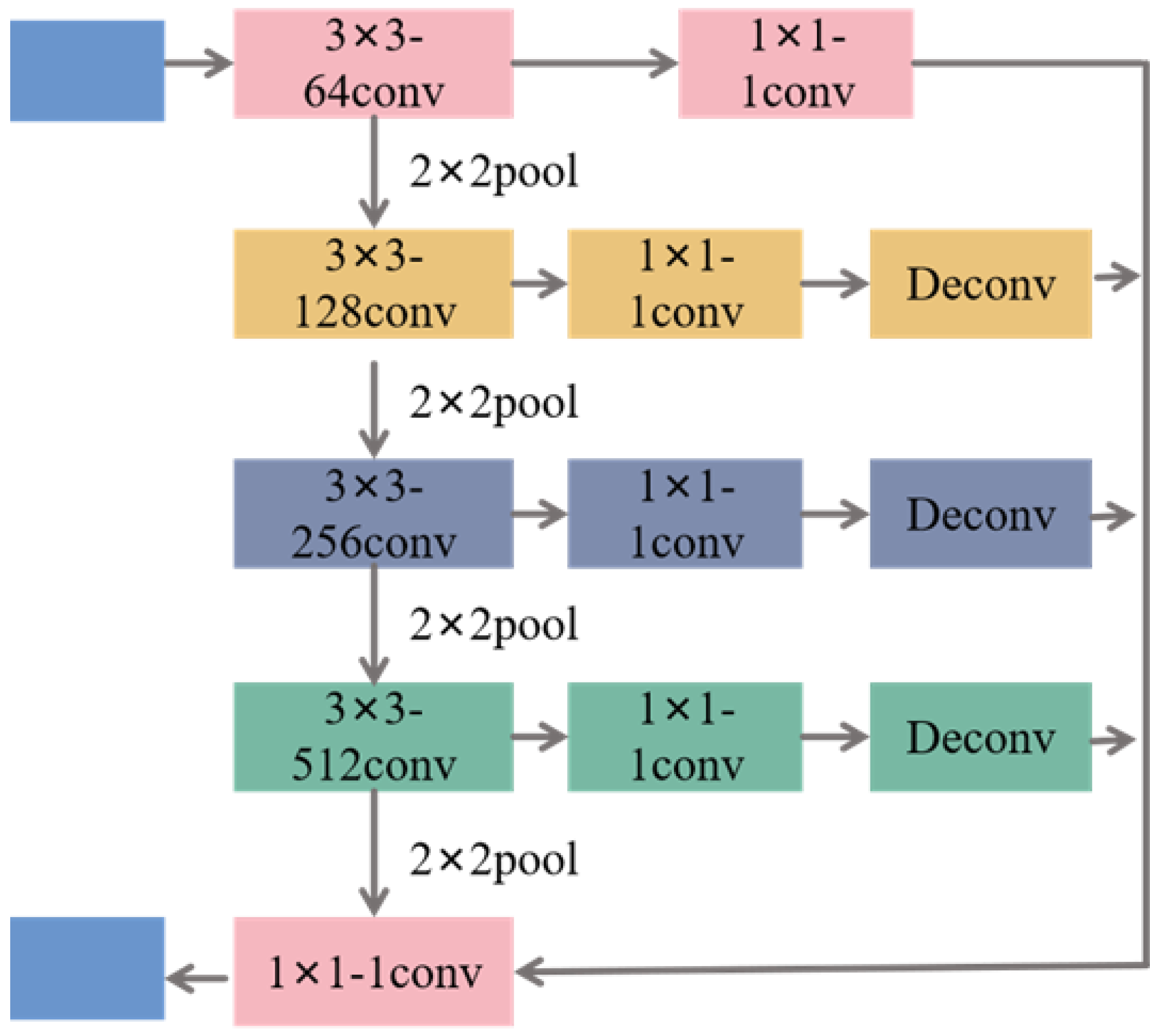
This article constructs a network structure, as shown in Figure 1, based on the Unet network architecture. The network has three parts: an edge detection sub-network (ED), an Unet semantic segmentation sub-network, and a feature fusion module.

The implementation steps of EDFF-Unet mainly include: (1) changing the downsampling of the semantic segmentation sub-network to an improved ASPP spatial pyramid pooling module and embedding an attention mechanism module (CBAM) into the skip connections to obtain semantic segmentation feature maps through upsampling; (2) obtaining the contour feature information of the input image through four consecutive convolutional layers in the edge detection (ED) sub-network, thereby obtaining the edge detection feature map; (3) using the feature fusion module (FF) to weigh and fuse the input feature map, semantic segmentation feature map, and edge detection feature map. Then, global average pooling and global max pooling operations are applied to compute spatial statistics for each feature channel. Finally, the weighted features are processed by a $1\times 1$ convolutional layer and normalized via a Sigmoid activation function to generate the refined output image.

2.2. Edge Detection Subnet (ED)

A branch network for edge feature extraction was designed to address the issues of target edge blurring and the loss of edge information during cloud shadow segmentation. This network synchronizes the semantic segmentation task with the edge feature extraction task. The edge detection sub-network extracts visually significant edges and object boundaries from images to obtain boundary information of cloud shadows and perform a more accurate semantic segmentation of images. The detailed network structure of the edge detection sub-network is shown in Figure 2.

In the edge detection sub-network, the convolutional layers are divided into four stages, with a $2\times 2$ pooling layer inserted between each convolutional stage to reduce the dimensionality of the extracted features. The first convolutional layer employs a $3\times 3$ kernel initialized via He normal initialization. The second, third, and fourth convolutional layers also use $3\times 3$ kernels. To maintain spatial consistency with the input image, a $1\times 1$ convolutional operation is applied at each stage, followed by a deconvolution operation to restore the feature map resolution. Finally, the feature maps obtained from the four stages are fused through a $1\times 1$ convolution operation and Sigmoid activation function. This can effectively obtain the contour of the image and obtain more precise and more complete edge information of the image target.

For the input feature map,

$$F_i={\mathrm{c}\mathrm{o}\mathrm{n}\mathrm{v}}_{k_i,c_i}({pool}_p\left(F_{i-1}\right))$$

(1)

$$D_i={\mathrm{D}\mathrm{e}\mathrm{c}\mathrm{o}\mathrm{n}\mathrm{v}}_d{(\mathrm{c}\mathrm{o}\mathrm{n}\mathrm{v}}_{1\times 1}({pool}_p\left(F_i\right)))$$

(2)

$$F_{out}=F_{i-1\text{\_}out}+D_i$$

(3)

where $i$ represents the number of network layers and $i=1,2,3,4$. $k_i$ indicates the size of the convolutional kernel at the layer level $i$; $c_i$ indicates the number of output channels for the convolutional layer $i$; $p$ indicates the size of the pooling kernel; and $d$ represents the size of the deconvolution kernel.

2.3. Attention Mechanism CBAM

CBAM, as an adaptive feature importance learning mechanism widely used in convolutional neural networks, can improve network performance. When given a feature map, the module autonomously infers attention weight values along two independent dimensions and then multiplies the generated attention weight map by the input feature map for adaptive refinement processing. The structure of CBAM is shown in Figure 3.

This mechanism consists of two parts—a channel attention module and a spatial attention module. The channel attention module learns and highlights the importance of each channel in feature extraction through weighted averaging processing. By using global average pooling and global max pooling (where the pooling kernel size equals the spatial dimensions of the input feature map), the spatial dimensions of the input features are compressed to 1, generating two channel descriptors. These descriptors are then fed into a shared multi-layer perceptron (MLP) for feature transformation, producing a channel attention map. Finally, the values of the attention map are normalized to the range [0, 1] via a Sigmoid function. The spatial attention module learns and emphasizes the importance of each spatial position in feature extraction through weighted averaging, effectively highlighting the target area and suppressing irrelevant information. By performing channel-wise average pooling and max pooling on the input feature map (assuming the input feature map is $\mathrm{H}\times \mathrm{M}\times \mathrm{C}$, which becomes $1\times \mathrm{M}\times \mathrm{C}$ after average pooling, while max pooling retains $1\times \mathrm{M}\times \mathrm{C}$), two spatial descriptors are obtained. These descriptors are concatenated along the channel dimension and fed into a 7 × 7 convolutional layer to generate a spatial attention map. Finally, the values of the spatial attention map are normalized to the range [0, 1] via a Sigmoid function. Through the above mechanism, the influence of noise in cloud images can be reduced, important regional features can be highlighted, and the segmentation effect of clouds and cloud shadows can be improved. The operation process of CBAM fusion attention can be defined as

$$F_c=\sigma (MLP\left(AvgPool\left(X\right)\right)+MLP\left(MaxPool\left(X\right)\right))$$

(4)

$$F_m=X\odot F_c$$

(5)

$$F_s=\sigma (\mathrm{C}\mathrm{o}\mathrm{n}\mathrm{v}\left((AvgPool\left(F_m\right);MaxPool\left(F_m)\right)\right)$$

(6)

$$F_{\mathrm{C}\mathrm{B}\mathrm{A}\mathrm{M}}=F_m\odot F_s$$

(7)

where $X$ represents the input feature map; $\sigma$ represents the Sigmoid function; $F_c$ represents the feature map after channel attention; $F_m$ is the input characteristic graph of spatial attention; $F_s$ represents the feature map after spatial attention; the “;” in Formula 6 represents concatenating $AvgPool\left(F_m\right)$ and $MaxPool\left(F_m)\right)$ in the channel dimension; the “$\odot$” in Formulas (5) and (7) represents the Hadamard product; and $F_{\mathrm{C}\mathrm{B}\mathrm{A}\mathrm{M}}$ represents the weight feature vector output after CBAM fusion attention operation.

2.4. Improved ASPP Hollow Space Pyramid Pooling Module

The Unet network can capture features at different levels through an encoder–decoder structure, but its ability to extract multi-scale information is relatively limited. In the encoder stage, it mainly focuses on extracting local information, while in the decoder stage, although upsampling and feature fusion are performed, it may still be difficult to effectively integrate local information with global information, resulting in insufficient utilization of receptive fields and affecting the understanding of the overall structure and target of the image.

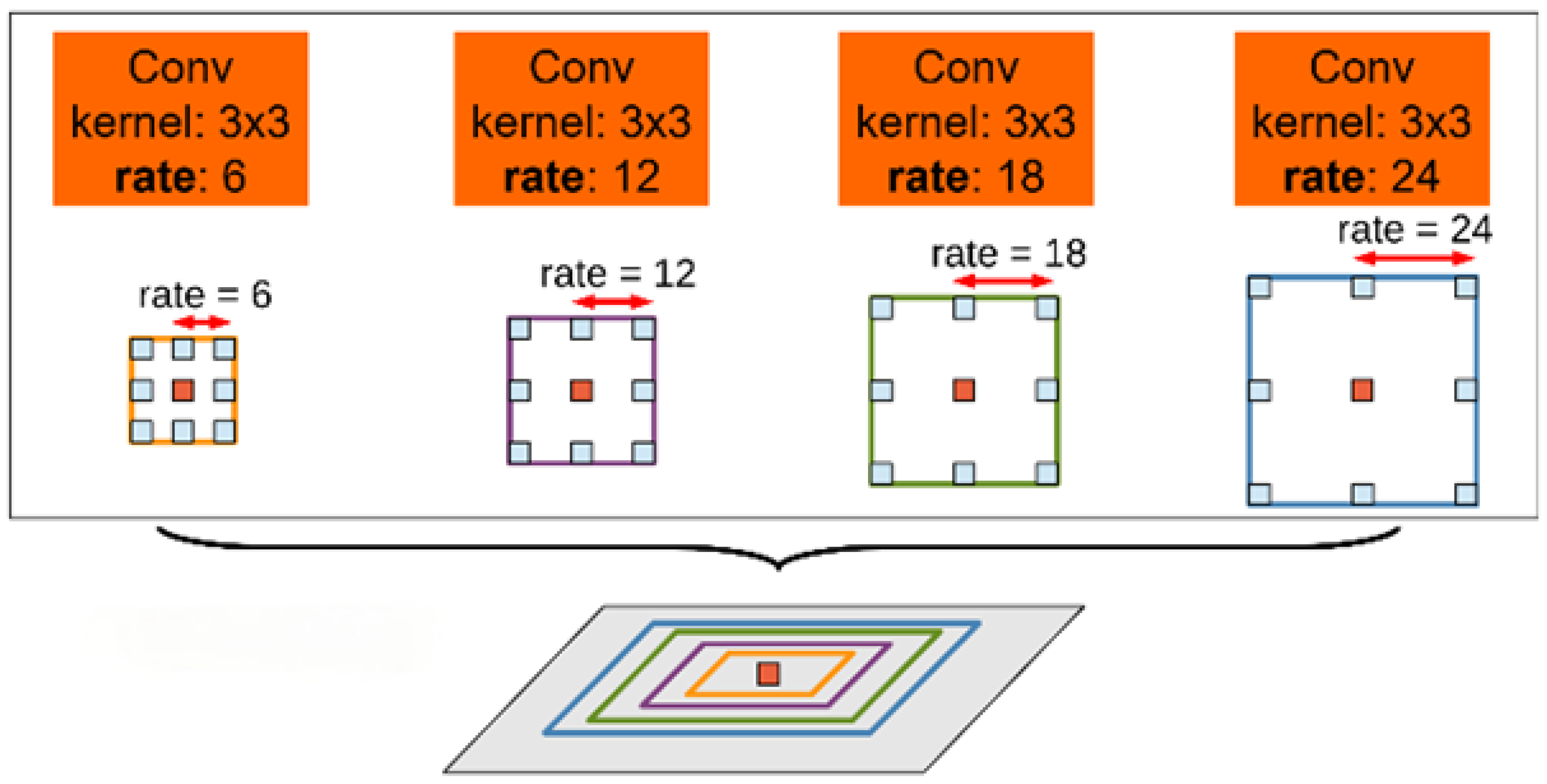
Hollow convolution [18] has always been favored by researchers in the field of segmentation as a means of effectively expanding the receptive field of ordinary convolution kernels. Its ability lies in significantly expanding the receptive field of the convolutional kernel without increasing the number of model parameters and computational complexity. As shown in Figure 4, adding intervals to a regular convolution kernel to form a dilated convolution allows the kernel to cover a larger range without changing the size or number of layers. The relationship between the convolution kernel’s range of dilated convolution and its dilation rate is shown in the Formula (8).

$$F=k+(k-1)\times (r-1)$$

(8)

where $r$ is the void rate; $k$ is the range of the initial convolution kernel; and $F$ is the actual receptive field size of dilated convolution.

Therefore, the plan is to change the downsampling operation of the original Unet network to the ASPP atrous space pyramid pooling module. This module originally included four parallel $3\times 3$ convolutions with different hole rates, expanding the receptive field of the convolution kernel and obtaining contextual information of the image at multiple scales through a dimensionality reduction in input features. Its structure is shown in Figure 5.

However, the original ASPP lacked the balanced processing of local and global features, resulting in the insufficient extraction of some information. Therefore, this paper adds an Avgpool and a Maxpool to the ASPP module.

• AvgPool: By averaging the local regions of the feature map, more global contextual information can be retained, which helps the network capture the overall structure of the image.
• MaxPool: By performing maximum value operations on local regions of the feature map, more local detail information can be preserved, which helps the network capture detailed features such as the edges and textures of the image.

By combining AvgPool and MaxPool, the module can simultaneously preserve global contextual information and local detail information, thereby achieving a better balance in the feature extraction process. This combination can enhance the network’s ability to extract multi-scale features, especially when dealing with complex segmentation tasks, and to better cope with targets of different scales. Considering that the feature maps of AvgPool and MaxPool may not be consistent in scale and semantics, in the improved ASPP, the output feature maps of AvgPool and MaxPool will undergo a $1\times 1$ convolution for channel adjustment and semantic alignment, and then be fused by element-wise addition or channel concatenation, supplemented by batch normalization (BatchNorm) and activation function (ReLU), to ensure that features from different sources have consistent scale and semantic expression before fusion, thereby avoiding information conflicts. The improved ASPP is shown in Figure 6.

The improved ASPP process is as follows: (1) The first convolutional layer employs a $1\times 1$ convolutional kernel to perform preliminary feature extraction on the input feature map, generating initial representations of cloud patterns. (2) The second convolutional layer utilizes a $3\times 3$ convolutional kernel with a dilation rate of 6, enabling the capture of broader contextual information across larger spatial regions in the feature map. (3) The third convolutional layer adopts a $3\times 3$ kernel with an increased dilation rate of 12, further expanding the receptive field to extract large-scale features that characterize interactions between clouds and their shadows. (4) The fourth convolutional layer incorporates a $3\times 3$ kernel with a maximum dilation rate of 18, facilitating the extraction of the most extensive contextual information from the feature map. (5) The max pooling layer operates on local regions of the input feature map by selecting maximum values, thereby enhancing sensitivity to abrupt intensity variations and precisely capturing fine-grained shadow boundaries through localized detail preservation. (6) The average pooling layer computes spatial averages over local regions, effectively suppressing noise while stabilizing global contextual information, which is critical for the robust identification of large-scale shadow regions. (7) The fusion layer concatenates feature maps from different convolutional and pooling layers, and the $1\times 1$ convolutional layer convolves the fused feature maps to obtain the result.

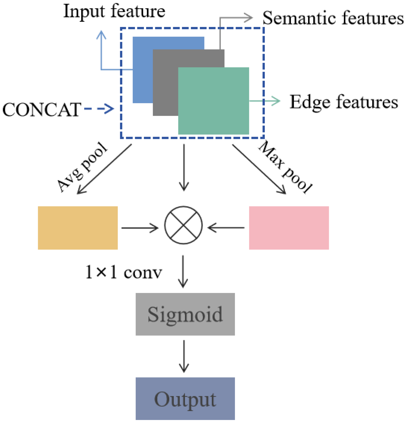
2.5. Feature Fusion Module (FF)

When the semantic segmentation sub-network and the edge detection sub-network extract semantic features and edge features, respectively, they are fused. The concat fusion method can fully preserve the original information of each participating feature map without losing features. Therefore, this paper designs a feature fusion module based on the concat fusion method to weigh and fuse the two features. The structure of the feature fusion module is shown in Figure 7.

In the feature fusion module, the input feature map, semantic feature map, and edge feature map are first concatenated and fused. The number of channels for the input feature map, semantic feature map, and edge feature map is ${\mathrm{C}}_1, {\mathrm{C}}_2$, and ${\mathrm{C}}_3$. The spatial dimensions are all $\mathrm{H}\times \mathrm{M}$. After splicing, the number of channels in the fused feature map is $\mathrm{C}={\mathrm{C}}_1+{\mathrm{C}}_2+{\mathrm{C}}_3$, and the spatial dimension remains $\mathrm{H}\times \mathrm{M}$. Then, the global average of the corresponding feature channels is obtained through average pooling and max pooling operations. Both global average pooling and maximum pooling use spatial global pooling, with an output dimension of $1\times 1\times \mathrm{C}$. And the weights of the feature channels are allocated through multiplication calculation to extract adequate feature information. Then, using a $1\times 1$ convolution operation to perform channel dimensionality reduction on the features, integrating cross-channel information through linear transformation, the spatial dimension of the output feature map remains $\mathrm{H}\times \mathrm{M}$. Finally, the Sigmoid classifier is used for prediction to obtain the final result. The calculation process of the multiplication is shown in Formula (9).

$$y_i={\displaystyle \sum _{k=1}^N}{\omega }_i{x}_k$$

(9)

where $y_i$ represents the feature value of the th channel on the weighted fused feature map; $x_k$ represents the feature value of the $k$ channel on the feature map; ${\omega }_i$ represents the weight coefficient of the $i$ channel; and $N$ represents the number of feature channels.

3. Experiment

3.1. GF1_WHU Dataset

GF1_WHU (GF-1 Cloud and Cloud Shadow Coverage Verification Dataset) [19] was released by the SENSIMAGE Laboratory at Wuhan University and is widely used in cloud detection and cloud shadow segmentation tasks. This dataset includes 108 GF-1 Wide Field of View (WFV) 2A level images and their corresponding reference masks collected from May 2013 to August 2016. The corresponding ground truth masks are divided into four categories: background pixels are 0, transparent area pixels are 1, cloud shadow area pixels are 128, and cloud area pixels are 255. Each image in the dataset consists of four multispectral bands, including three visible R, G, and B bands and one near-infrared band, with a spatial resolution of 16 m. All four multispectral bands of the GF1_WHU dataset were utilized for cloud detection. The combination of multi-band information is beneficial for improving the accuracy of cloud and cloud shadow detection. As shown in Figure 8, the GF1_WHU dataset contains images of different cloud types (such as cumulus, stratus, cirrus, etc.), cloud cover, cloud shadow patterns, and different geographical environments. The data types and contents are rich and diverse, providing sufficient materials for this study.

3.2. HRC_WHU Dataset

HRC_WHU (High Resolution Classification Dataset of Wuhan University) is a high-precision remote sensing image semantic segmentation benchmark dataset released by the School of Remote Sensing Information Engineering of Wuhan University. It is designed for tasks such as building extraction and land use classification, and consists of 150 high-resolution remote sensing images with resolutions mainly ranging from 0.5 to 15 m. The original size is 1280 × 720. This dataset covers multiple urban scenes in China, including diverse geographical environments such as cities, suburbs, and rural areas.

3.3. Evaluating Indicator

The experiment evaluates the effectiveness of the model using four indicators—pixel accuracy (PA), average pixel accuracy (MPA), F1, and the mean intersection-to-union ratio (MIOU). The specific calculation formulas are as follows:

PA is defined as the proportion of correctly classified pixels to all pixels.

$$PA={\displaystyle \frac{\sum _{i=0}^k{p}_{ii}}{\sum _{i=0}^k\sum _{j=0}^k{p}_{ij}}}$$

(10)

MPA is computed by the ratio of the number of correctly classified pixels for each class to the total number of pixels for that class, and then the average is taken.

$$MPA={\displaystyle \frac{1}{k}}\sum _{i=0}^k{\displaystyle \frac{P_{ii}}{\sum _{j=0}^k{p}_{ij}}}$$

(11)

F1 is the harmonic mean of accuracy and recall, reflecting the overall performance of the model.

$$F1={\displaystyle \frac{1}{k+1}}\sum _{i=0}^k{\displaystyle \frac{2\times {TP}_i}{2\times {TP}_i+{FP}_i+{FN}_i}}$$

(12)

MIOU measures the degree of overlap between predicted and actual cloud and shadow regions.

$$MIoU={\displaystyle \frac{1}{k+1}}\sum _{i=0}^k{\displaystyle \frac{p_{ii}}{{\sum }_{j=0}^k{p}_{ij}+{\sum }_{j=0}^k{p}_{ji}-p_{ii}}}$$

(13)

in Formulas (10)–(13) above, $k+1$ is the number of categories; $p_{ii}$ is the class $i$ pixel and is predicted to be the number of class $i$ pixels; $P_{ij}$ is the class $i$ pixel and is predicted to be the number of class $j$ pixels; $p_{ji}$ is the class $j$ pixel and is predicted to be the number of class $i$ pixels; ${TP}_i$ indicates that the $i$ sample is correctly divided into cloud and cloud shadow; ${FP}_i$ indicates that the $i$ sample background pixel is incorrectly divided into cloud and cloud shadow; and ${FN}_i$ indicates that the cloud and cloud shadow of sample $i$ are wrongly divided into background pixels.

This study also introduces an evaluation metric—Border Intersection Union (Border IoU), which is used to evaluate the accuracy of target boundary regions in image segmentation. Its calculation formula is as follows:

Expand the boundaries of the Ground Truth (GT) and Prediction (Pred) masks through morphological dilation to generate boundary regions of a specified width:

$$\mathrm{G}\mathrm{T}\text{\_}\mathrm{b}\mathrm{o}\mathrm{r}\mathrm{d}\mathrm{e}\mathrm{r}=\mathrm{D}\mathrm{i}\mathrm{l}\mathrm{a}\mathrm{t}\mathrm{i}\mathrm{o}\mathrm{n}(\mathrm{G}\mathrm{T},\mathrm{d})-\mathrm{G}\mathrm{T}$$

(14)

$$\mathrm{P}\mathrm{r}\mathrm{e}\mathrm{d}\text{\_}\mathrm{b}\mathrm{o}\mathrm{r}\mathrm{d}\mathrm{e}\mathrm{r}=\mathrm{D}\mathrm{i}\mathrm{l}\mathrm{a}\mathrm{t}\mathrm{i}\mathrm{o}\mathrm{n}(\mathrm{P}\mathrm{r}\mathrm{e}\mathrm{d},\mathrm{d})-\mathrm{p}\mathrm{r}\mathrm{e}\mathrm{d}$$

(15)

where $\mathrm{G}\mathrm{T}\text{\_}\mathrm{b}\mathrm{o}\mathrm{r}\mathrm{d}\mathrm{e}\mathrm{r}$ represents the true boundary area; $\mathrm{P}\mathrm{r}\mathrm{e}\mathrm{d}\text{\_}\mathrm{b}\mathrm{o}\mathrm{r}\mathrm{d}\mathrm{e}\mathrm{r}$ represents the predicted boundary region; “$\mathrm{D}\mathrm{i}\mathrm{l}\mathrm{a}\mathrm{t}\mathrm{i}\mathrm{o}\mathrm{n}()$” represents morphological dilation operation; and $\mathrm{d}$ represents the expansion radius.

$$\mathrm{B}\mathrm{o}\mathrm{r}\mathrm{d}\mathrm{e}\mathrm{r}\mathrm{}\mathrm{I}\mathrm{o}\mathrm{U}={\displaystyle \frac{\sum \mathrm{G}\mathrm{T}\text{\_}\mathrm{b}\mathrm{o}\mathrm{r}\mathrm{d}\mathrm{e}\mathrm{r}\cap \mathrm{P}\mathrm{r}\mathrm{e}\mathrm{d}\text{\_}\mathrm{b}\mathrm{o}\mathrm{r}\mathrm{d}\mathrm{e}\mathrm{r}}{\sum \mathrm{G}\mathrm{T}\text{\_}\mathrm{b}\mathrm{o}\mathrm{r}\mathrm{d}\mathrm{e}\mathrm{r}\cup \mathrm{P}\mathrm{r}\mathrm{e}\mathrm{d}\text{\_}\mathrm{b}\mathrm{o}\mathrm{r}\mathrm{d}\mathrm{e}\mathrm{r}}}$$

(16)

3.4. Hyperparametric Experiment

This article adopts a joint loss function strategy as the loss function, using Dice coefficient loss and smoothed version L1 loss in combination. The joint use of these two loss functions can optimize model performance at multiple levels, ensuring both the overlap of segmentation regions and the better spatial fit of predicted segmentation regions to the actual region. At the same time, it also considers the measurement of the difference between predicted and actual values at the pixel level, thereby ensuring pixel-level accuracy. This joint loss function helps the segmentation results to be more in line with the actual situation in terms of details while ensuring the reliable performance of the model in segmentation tasks with different scale structures. Cloud and shadow boundaries often exhibit irregularity, and joint loss can ensure approximate coverage of the cloud shadow area through Dice loss, while constraining the offset error of boundary pixels through Smooth L1 loss. The specific formula is as follows:

$$L=\alpha {Lose}_{Dice}+\beta {Lose}_{SmoothL1}$$

(17)

where $\alpha$ and $\beta$ represent weight coefficients, ${Lose}_{Dice}$ represents the Dice coefficient loss function, and ${Lose}_{SmoothL1}$ represents the smooth version L1 loss function.

The Dice coefficient is an indicator used to measure the similarity between two sets. Especially in the field of image segmentation processing, the Dice coefficient is used as a loss function to help evaluate the similarity between predicted results and actual results. The Dice coefficient is based on the size of two sets and the size of their intersection. Given the two sets A and B, the Dice coefficient formula is as follows:

$$Dice={\displaystyle \frac{2\left|A\cap B\right|}{\left|A\right|+\left|B\right|}}$$

(18)

The Dice loss function is a loss function based on the Dice coefficient, which aims to minimize the Dice coefficient and improve the similarity between the segmentation result and the actual label. In practical applications, continuous probability values are usually used instead of binary results, and to avoid dividing by zero, a small smoothing term $\epsilon$ is added to the formula. Therefore, the Dice coefficient loss function in this article is expressed as:

$${Lose}_{Dice}=1-{\displaystyle \frac{2{\sum }_{i=1}^N{p}_i{t}_i+\epsilon }{{\sum }_{i=1}^N\left(p_i^2+t_i^2\right)+\epsilon }}$$

(19)

where $p_i$ and $t_i$ represent the predicted value and true value of the $i$ pixel.

The SmoothL1 loss function is a combination of L1 loss and L2 loss. When the difference between the predicted value and the actual value is small (less than beta, assumed to be 1.0 here), its calculation method is similar to L2 loss (squared error); when the difference is significant, its calculation method is similar to L1 loss (absolute error), enhancing the robustness of the model to outliers. Near zero, the gradient of the SmoothL1 loss function is continuous and smoothly changing, which makes the parameter updates of the model more stable and continuous during the training process. SmoothL1Loss is represented as:

$${Lose}_{SmoothL1}=\left\{\begin{array}{c}0.5{(x-y)}^{2}if\left|x-y\right|<1\hfill \\ \left|x-y\right|-0.5otherwise\hfill \end{array}\right.$$

(20)

where $x$ represents the output of the model and $y$ represents the label of the model.

Experiments were conducted with different weights, and the performance comparison and quantification results of different weights are shown in

Table 1. Comparison of same weight performance in tables (%).

$\mathsf{\alpha }$	$\mathsf{\beta }$	PA	MPA	F1	MioU
0	1	94.67	93.27	93.59	91.37
0.2	0.8	94.66	94.09	93.74	91.26
0.4	0.6	95.79	94.87	94.36	91.11
0.6	0.4	96.02	95.33	95.28	92.63
0.8	0.2	96.11	95.37	95.54	92.87
1	0	96.04	95.19	95.41	92.68

:

By continuously adjusting the value of $\alpha$ and $\beta$ to analyze the network performance, the optimal extraction accuracy can be obtained. The PA, MPA, F1, and MioU indexes of the model performance are evaluated. It can be seen from Table 1 that when $\alpha =0.8$, $\beta =0.2$, the evaluation index was the highest and the image segmentation effect was the best.

3.5. Ablation Experiment

In order to verify the effectiveness of each module in this method, ablation experiments were conducted on the edge detection module, attention mechanism module, and hollow space pyramid pooling module. MioU, PA, and MPA were used as the evaluation criteria for experimental effectiveness. The specific experimental results are shown in

Table 2. Performance on GF1_WHU dataset (%).

Serial Number	edge	cbam	aspp	PA	MPA	MioU
1	×	×	×	89.67	89.21	88.09
2	√	×	×	93.06	90.87	89.33
3	×	√	×	93.11	91.96	89.56
4	×	×	√	93.85	92.65	89.74
5	√	√	×	95.01	93.93	91.21
6	√	×	√	94.19	94.33	91.01
7	×	√	√	94.06	95.32	90.87
8	√	√	√	96.11	95.37	92.87

. Where √ represents adding the module, and × represents not adding the module.

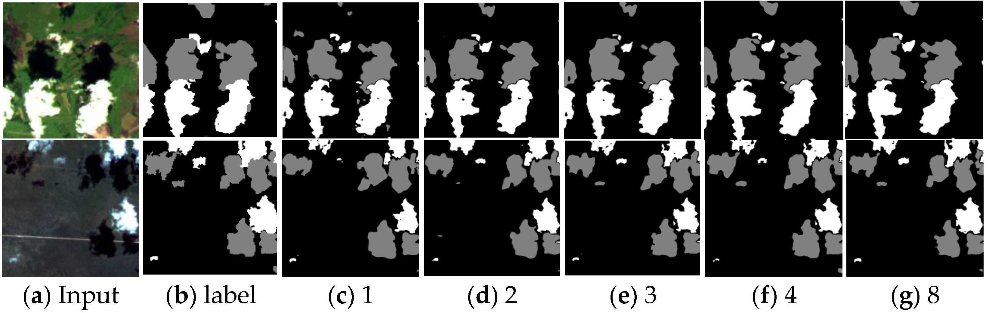
Table 2 experimental results show that the indicators of the edge detection module, attention mechanism module, and hollow space pyramid pooling module are improved by adding them separately. When the two modules are added at the same time, the best effect is achieved. When the edge detection module, attention mechanism module, and hollow space pyramid pooling module are added at the same time, PA, MPA, and MioU are increased by 5.54%, 6.96%, and 3.96%, respectively. This shows that embedding an edge detection module, attention mechanism module, and hollow space pyramid pooling module into the basic feature extraction network has a good effect on improving the accuracy of the model.

From the visualization results of the ablation experiment in Figure 9, it can be further seen that EDFF-Unet can significantly improve the segmentation performance of cloud and cloud shadow, and reduce missed detection and false detection.

To further validate the effectiveness of the feature fusion module, we selected the following three baseline methods for comparison:

• Direct addition fusion (Add): Directly add the input feature map, semantic feature map, and edge feature map element-by-element;
• Multiply element-by-element (Multiply): Multiply the input feature map, semantic feature map, and edge feature map element-by-element, and directly output the fused feature map;
• Attention fusion (Channel Attention): Introducing a channel attention mechanism (SE Block) after concatenation to replace the pooling weight allocation strategy in this paper.

All feature maps are uniformly adjusted to the same spatial size through adaptive pooling, and mapped to a uniform number of channels through $1\times 1$ convolution to ensure the smooth experimentation of Add and Multiply. The experimental results were quantified using MIoU, and the results obtained from the GF1_WHU dataset are shown in

Table 3. Segmentation results under different fusion methods.

Methods	MIoU (%)
Add	88.09
Multiply	88.11
Channel Attention	90.24
FF	92.87

:

The experiment shows that the fusion feature module proposed in this paper exhibits good performance on the GF1_WHU dataset. Compared with other baseline methods, the fusion module in EDFF-Unet can improve the segmentation ability of cloud images.

Because edge detection is a prominent feature of this method, the effectiveness of edge detection will be validated for different cloud types. The study selects three different cloud types from the GF1_WHU dataset—cumulus clouds, stratus clouds, and cirrus clouds—to demonstrate the effectiveness of edge detection, and quantifies the experimental results of the edge detection using Border IoU.

The specific experimental results are shown in

Table 4. Performance on GF1_WHU dataset (%).

Types	Border IoU	MIoU
Cumulus clouds	93.11	92.88
Stratus clouds	93.41	92.57
Cirrus clouds	92.96	92.49

. From the table, it can be seen that the edge detection module has good detection performance for different types of cloud images, effectively enhancing boundary features. The segmentation accuracy (Border IoU) in the edge region is slightly better than the segmentation effect (MIoU) in the overall region, indicating that the edge detection model effectively improves the overall segmentation effect.

3.6. Experimental Results Display

The Table 2 experimental results show the indicators of the edge detection module, attention mechanism module, and improved ASPP. In order to evaluate the performance of the proposed network and verify the effectiveness and feasibility of EDFF-Unet, it was qualitatively and quantitatively compared with classical segmentation networks such as Unet, FCN, PAN, and the recent models ViT D-UNet and DBNet on the GF1_WHU dataset. The comparison results are shown in

Table 5. Performance on GF1_WHU dataset (%).

Model	PA	MPA	F1	MIoU
Unet	93.26	92.41	92.31	88.11
FCN	94.33	94.52	94.27	88.21
PAN	93.34	93.28	92.41	91.24
PSPNet [20]	95.21	94.49	95.29	90.93
CloudNet [21]	94.05	94.22	95.34	89.31
D-Unet	94.76	94.38	95.36	91.24
DABNet [22]	94.33	93.87	94.77	90.59
DeepLab V3plus [23]	95.12	95.05	95.09	90.55
LinkNet [24]	93.68	93.82	92.63	92.02
CGNet [25]	95.86	95.83	95.31	90.77
PVT [26]	93.63	93.77	92.53	91.89
CVT [27]	93.42	92.39	92.26	91.58
ViT-D-UNet [28]	95.07	95.14	95.33	91.97
DBNet [29]	94.47	94.26	94.54	90.62
EDFF-Unet	96.11	95.37	95.54	92.87

. From the table, it can be seen that, compared to other algorithms, the model proposed in this paper performs better in cloud and cloud shadow recognition. In addition to MPA, PA, F1, and MIoU are 0.25%, 0.18% and 0.67% ahead of the sub-excellent networks, respectively. The quantitative evaluation results show that the proposed method is more accurate and robust than other comparison methods and has a better segmentation ability for clouds and shadows with different shapes and distributions.

Figure 10 shows the visual comparison results of the GF1_WHU dataset. Compared with the current cutting-edge ViT-D-UNet and DBNet, the network proposed in this study shows higher detection accuracy in the fuzzy feature area and can more accurately define the target boundary. It is worth noting that this network still has excellent detection performance for targets of different sizes and irregular shapes.

As shown in Figure 11, this network reduces false detection and missed detection in target detection compared with other existing networks. In the figure, the green rectangular area indicates correct detection, and the red rectangular area indicates false detection and missed detection.

In order to further investigate the performance of the model and verify its generalization, this study compares multiple datasets [30,31,32] and ultimately chooses the HRC_WHU dataset. The HRC_WHU dataset has cloud images that are not consistent in style with the GF1_WHU dataset, such as the cloud images with dense building obstructions in the HRC_WHU dataset. The model in this article was compared with some popular models and the experimental results are shown in

Table 6. Performance on HRC_WHU dataset (%).

Model	PA	MPA	F1	MIoU
Unet	89.33	88.94	88.13	84.09
FCN	90.26	90.11	88.36	84.16
PAN	89.79	89.64	89.83	86.05
PSPNet	90.42	90.79	89.59	86.01
CloudNet	90.11	91.09	90.92	84.57
D-Unet	91.23	91.58	90.89	86.61
DABNet	91.41	90.31	89.57	85.73
DeepLab V3plus	92.47	91.49	91.01	85.56
LinkNet	90.51	90.55	91.05	87.02
CGNet	91.67	91.13	91.46	85.27
PVT	91.26	90.67	89.92	86.87
CVT	91.58	91.03	90.84	86.60
ViT-D-UNet	92.19	91.27	91.67	86.33
DBNet	92.02	90.96	91.21	85.83
EDFF-Unet	92.87	92.03	91.85	87.36

:

From the results, EDFF-Unet still maintains optimal performance on the HRC_WHU dataset. The model still leads by 0.34% in the MIoU metric.

In order to verify the effectiveness and accuracy of the edge detection module in this study, comparative experiments were conducted on the edge detection performance of different networks, and Border IoU and MIoU were used to quantify the effect. Experiments were conducted on two datasets, the GF1_WHU dataset and the HRC_WHU dataset, and the experimental results are shown in

Table 7. Performance on GF1_WHU dataset and HRC_WHU dataset (%).

Model	GF1_WHU Dataset		HRC_WHU Dataset
	Border IoU	MIoU	Border IoU	MIoU
Unet	88.49	88.11	85.22	84.09
FCN	88.58	88.21	85.25	84.16
PAN	92.03	91.24	87.36	86.05
PSPNet	91.21	90.93	86.73	86.01
CloudNet	90.23	89.31	85.03	84.57
D-Unet	91.96	91.24	86.92	86.61
DABNet	91.84	90.59	86.83	85.73
DeepLab V3plus	91.82	90.55	85.94	85.56
LinkNet	92.78	92.02	88.15	87.02
CGNet	91.92	90.77	86.93	85.27
PVT	92.77	91.89	87.49	86.87
CVT	92.49	91.58	87.73	86.60
ViT-D-UNet	93.14	91.97	88.02	86.33
DBNet	91.63	90.62	86.85	85.83
EDFF-Unet	93.64	92.87	88.42	87.36

:

The experimental results show that, compared to other networks, the edge detection module EDFF-Unet has better performance and good accuracy. On the GF1_WHU and HRC_WHU datasets, EDFF-Unet has the highest Border IoU and MIoU, demonstrating its strong ability to capture complex boundaries and multi-scale features in remote sensing images. On the GF1_WHU dataset, the Border IoU reached 93.64%, which is 0.5% higher than the Border IoU value of the next best network; on the HRC_WHU dataset, the Border IoU reached 88.42%, which is 0.3% higher than the Border IoU value of the next best network.

On the basis of the above comparative experiments, it can be concluded that EDFF-Unet has a superior segmentation ability. In order to further verify the performance of EDFF-Unet and eliminate the influence of chance, this study continues to use an independent two-sample t-test to demonstrate the statistical test results, supporting the conclusion that EDFF-Unet has superior performance. Conduct 3 tests on EDFF-Unet and the comparison model on the GF1_WHU dataset, and calculate the average MIoU of the three experiments and the mean difference in the EDFF-Unet compared to each comparison model $∆\mathsf{\mu }$ (Average MIoU of EDFF-Unet—Average MIoU of the comparison model). By checking the normality and homogeneity of the variance of the data, it was found that the data follows a normal distribution and has homogeneity of variance, meeting the conditions of an independent two-sample t-test. The specific steps are as follows:

• Set the null hypothesis and alternative hypothesis: The null hypothesis ($H_0$)—there is no significant difference in the mean performance indicators between EDFF-Unet and the comparable model. Alternative hypothesis ($H_1$)—EDFF-Unet performs significantly better than the comparison model.
• Set significance level: Set $\mathsf{\alpha }$ = 0.05; if $p<\mathsf{\alpha }<0.05$, reject the null hypothesis.
• Calculate t(df) and $P$ to determine significance.

  $$\mathrm{t}={\displaystyle \frac{∆\mathsf{\mu }}{\sqrt{\frac{{\mathsf{\sigma }}_{\mathrm{E}\mathrm{F}-\mathrm{U}\mathrm{n}\mathrm{e}\mathrm{t}}^2}{3}+\frac{{\mathsf{\sigma }}_{\mathrm{c}\mathrm{o}\mathrm{n}\mathrm{t}\mathrm{r}\mathrm{a}\mathrm{s}\mathrm{t} \mathrm{m}\mathrm{o}\mathrm{d}\mathrm{e}\mathrm{l}}^2}{3}}}}$$

  (21)

  where ${\mathsf{\sigma }}_{\mathrm{E}\mathrm{F}-\mathrm{U}\mathrm{n}\mathrm{e}\mathrm{t}}^2$ represents the variance of mIoU values for EDFF-Unet in three tests; ${\mathsf{\sigma }}_{\mathrm{c}\mathrm{o}\mathrm{n}\mathrm{t}\mathrm{r}\mathrm{a}\mathrm{s}\mathrm{t} \mathrm{m}\mathrm{o}\mathrm{d}\mathrm{e}\mathrm{l}}^2$ represents the variance of mIoU values for the comparable model in three tests.

The experimental results are shown in the following

Table 8. Independent two-sample t-test experimental results.

Model	Test 1 (%)	Test 2 (%)	Test 3 (%)	Average MioU (%)	$∆\mathsf{\mu }$ (%)	$\mathit{p}$	$\mathbf{S}\mathbf{i}\mathbf{g}\mathbf{n}\mathbf{i}\mathbf{f}\mathbf{i}\mathbf{c}\mathbf{a}\mathbf{n}\mathbf{c}\mathbf{e}$
Unet	88.11	88.34	88.01	88.15	4.51	0.002	yes
FCN	88.21	88.56	88.44	88.40	4.26	0.004	yes
PAN	91.24	90.87	90.16	90.76	1.9	0.027	yes
PSPNet	90.93	90.64	89.91	90.50	2.16	0.009	yes
CloudNet	89.31	90.04	90.39	89.91	2.75	0.008	yes
D-Unet	91.24	91.31	91.33	91.29	1.37	0.031	yes
DABNet	90.59	90.61	89.86	90.35	2.31	0.010	yes
DeepLab V3plus	90.55	91.02	91.29	90.95	1.71	0.022	yes
LinkNet	92.02	91.70	91.06	91.59	1.07	0.037	yes
CGNet	90.77	90.68	91.13	90.86	1.8	0.025	yes
PVT	91.89	91.64	90.77	91.43	1.23	0.029	yes
CVT	91.58	91.25	91.50	91.44	1.22	0.031	yes
ViT-D-UNet	91.97	92.06	92.03	92.02	0.64	0.042	yes
DBNet	90.62	90.64	91.71	90.99	1.67	0.023	yes
EDFF-Unet	92.87	92.91	92.21	92.66	0	none	none

. Through repeated experiments, independent two-sample t-tests, and result visualization, this analysis has verified the statistical significance of the performance advantages of EDFF-Unet. EDFF-Unet has superior detection and segmentation capabilities compared to other comparable networks.

4. Discussion

This study proposes EDFF-Unet, a semantic segmentation model for remote sensing image cloud and cloud shadow segmentation tasks, consisting of an edge detection module, a semantic segmentation module, and a feature fusion module. The segmentation performance of EDFF-Unet on cloud images can be well verified through ablation experiments, comparative experiments, etc., and it has good generalization ability. Subsequent experiments can be extended to other remote sensing segmentation tasks, such as water extraction and building detection [33,34,35]. However, there are still some challenges, such as differences in data labeling standards for different tasks (such as the soft/hard labeling of water boundaries), which may affect the effectiveness of model transfer [36]. Therefore, it is necessary to design task adaptive loss functions to ensure segmentation performance.

5. Conclusions

The EF-Uet model uses a semantic segmentation sub-network and edge detection sub-network to segment cloud and cloud shadow images. Then, a feature fusion module is used to realize the fusion of semantic features and edge features. The attention mechanism and the improved ASPP hole space pyramid pool module are deployed in the semantic segmentation sub-network so that the model can adaptively adjust the feature expression of cloud and cloud shadow feature maps and improve the ability of the model to capture key information. At the same time, abundant multi-scale information is captured at the local feature level, which effectively reduces the number of parameters compared with the ordinary convolution operation. The fusion of edge features and semantic features effectively improves the ability of the edge feature extraction of the model and obtains more precise and complete image target edge information. The comparative reality of the GF1_WHU dataset experiment verifies the network’s good performance. Compared with the initial model, the PA, MPA, F1, and MIoU indexes of the algorithm in this paper are improved by 2.85%, 2.96%, 3.23%, and 4.76%, respectively. In terms of the visual image segmentation results, the model achieved accurate segmentation results for the edge, fuzzy, and abstract features. Future research will try some new architectures, such as transformer-based architecture fusion, to analyze image features from different angles and further improve segmentation performance in complex scenes.