SCRM-Net: Self-Supervised Deep Clustering Feature Representation for Urban 3D Mesh Semantic Segmentation

Abstract

Semantic urban 3D meshes obtained by deep learning networks have been widely applied in urban analytics. Typically, a large amount of labeled samples are required to train a deep learning network to extract discriminative features for the semantic segmentation of urban 3D mesh. However, it is labor intensive and time consuming to obtain enough labeled samples due to the complexity of urban 3D scenes. To obtain discriminative features without extensive labeled data, we propose a novel self-supervised deep clustering feature learning network, named SCRM-Net. The proposed SCRM-Net consists of two mutually self-supervised branches: one branch utilizes autoencoder to learn intrinsic feature representations of urban 3D Mesh, while the other applies GCN to capture the structural relationships between them. During the semantic segmentation process, only a limited proportion of the labeled samples is required to fine-tune the pretrained encoder of SCRM-Net for discriminative feature extraction and to train the segmentation head consisting of two edge convolution layers. Extensive comparative experiments demonstrate the effectiveness of our approach and show its competitiveness against the state-of-the-art semantic segmentation methods.

1. Introduction

With the decline in the cost of 3D remote sensing data acquisition and the increased availability of such data, generating urban 3D mesh scene datasets has become feasible. The application of 3D mesh semantic segmentation networks offers substantial value across various domains, including urban planning [1], environmental monitoring [2], intelligent transportation [3], and automatic driving [4].

In the study of scene semantic segmentation, a significant number of deep-learning-based methods have been developed, primarily focusing on scene 3D point cloud datasets [5,6,7,8]. Compared to point clouds and other forms of 3D datasets, 3D mesh offers the advantage of continuous surfaces, enabling more precise capture of the topological structure and detailed shapes of complex urban scenes [9]. The strength of 3D mesh in representing high-precision geometric information makes it particularly suitable for fine-grained scene modeling. However, geometric information alone is insufficient to fully understand and utilize scene datasets. Therefore, achieving semantic segmentation information in urban 3D mesh is a promising research direction. Currently, few studies have focused on the semantic segmentation of 3D mesh urban scenes [10,11]. Moreover, the high cost of annotating large datasets and the significant variability in label consistency among different annotators further complicate the training and performance evaluation of deep learning models on large datasets. Compared to methods based on supervised learning, studies on 3D mesh semantic segmentation using self-supervised learning paradigms are notably lacking [9]. Thus, achieving accurate semantic segmentation of urban 3D mesh in the absence of extensive, detailed labeled datasets remains a highly challenging task.

As a branch of unsupervised learning, self-supervised learning employs various pretext tasks to automatically generate labels from data or to use intrinsic structural properties of the data as supervisory signals to learn useful representations [12,13]. This approach provides a promising learning paradigm for semantic segmentation on urban 3D mesh datasets. In recent years, end-to-end deep clustering representation learning methods have gradually gained widespread attention [12,14]. Deep clustering combines traditional clustering techniques with deep learning, extracting latent features from the data in a self-supervised manner to generate high-level general representations. However, applying deep clustering directly to urban 3D mesh representations presents several challenges. First, urban 3D meshes consist of complex geometric structures and diverse objects, making it difficult to extract meaningful features from the data. Second, the distribution of different object categories in urban scenes is often imbalanced, with buildings, for example, being far more numerous than smaller objects like cars. Effective feature selection is critical for achieving optimal clustering performance in urban 3D mesh. Deep clustering methods must be able to automatically select and extract effective features to enhance clustering performance and accuracy.

In this paper, we propose a self-supervised clustering-based representation learning network, SCRM-Net, specifically designed for feature representation learning on urban 3D meshes. The proposed SCRM-Net mainly consists of two mutually self-supervised branches: one branch employs an autoencoder to extract the inherent feature representations of the urban 3D mesh, while the other leverages a GCN to model the structural relationships within the data. Specifically, we selected samples with significant features as the basis for initializing clustering centers, rather than using the entire sample set. This approach is particularly important because the urban 3D mesh dataset contains millions of samples, many of which are redundant. Using the entire dataset may lead to feature redundancy, causing the clustering centers to focus more on local features while neglecting the global structure. Therefore, utilizing a subset of spatially distributed data not only reduces the computational overhead of initializing clustering centers but also better captures the global structure of the data. In contrast to methods that require complex geometric input representations for 3D mesh, we employed three types of common and easily obtainable 3D mesh features—normal vectors, centroid coordinates, and texture pixels of faces—as the network’s raw input. We designed an improved architecture incorporating an autoencoder and a graph encoder branch to represent the surface attributes and construct features of urban 3D mesh. To alleviate the over-smoothing issue of GCN in the graph encoder, we introduced skip connections in the encoding layers of the encoder. Additionally, to address the occasional noise present in the dataset, we incorporated normalization layers within the graph encoder and fused each layer of the autoencoder into the graph encoder, thereby achieving more stable feature representation. The overall network loss consists of reconstruction loss and clustering loss, ensuring that the network can efficiently learn and capture the structure and semantic features of urban 3D mesh.

The proposed method requires minimal labeled samples for fine-tuning the semantic segmentation head, reducing manual labor costs. Extensive ablation and comparative experiments are conducted on the public Semantic Urban Meshes (SUM) dataset [15]. The experimental results show that the proposed method achieves competitive accuracy compared to the state-of-the-art supervised semantic segmentation methods on urban 3D mesh.

In a nutshell, the main contributions of our method are summarized as follows:

• We propose a novel self-supervised deep clustering feature representation learning architecture for the semantic segmentation of urban 3D mesh.
• We enhance the structured deep clustering dual-branch network for high-level semantic representation learning and introduce a clustering center initialization method for imbalanced datasets. Additionally, we propose a subset sample fine-tuning strategy that accelerates fine-tuning after generating robust feature representations.
• Our SCRM-Net under the self-supervised learning framework demonstrates strong potential in urban 3D mesh scene semantic segmentation. Experimental results show that with only 10% labeled data for fine-tuning, SCRM-Net achieves segmentation accuracy comparable to existing supervised models, highlighting its competitive feature learning and generalization capabilities.

2. Related Works

In this section, we present the current state of research related to our work. We review the development of deep clustering and introduce the classical methods for 3D mesh semantic segmentation.

2.1. Deep Clustering Representation Learning

Unsupervised deep clustering methods have demonstrated outstanding performance in feature embedding, sparking widespread research and exploration [16,17,18,19]. Hinton et al. [20] were the first to propose the idea of using an autoencoder to compress high-dimensional data into low-dimensional representations, which laid the foundation for subsequent deep clustering algorithms. Deep clustering networks [21] combine dimensionality reduction (DR) with K-means clustering frameworks, enhancing both deep learning feature space optimization and clustering performance [22]. Existing surveys on self-supervised representation learning [23,24] have recognized deep clustering as a highly effective approach for representation learning, emphasizing its strong performance across various tasks. Therefore, leveraging deep clustering for 3D mesh representation learning presents a promising approach.

In recent years, inspired by the application of autoencoders [25] in unsupervised learning, various deep clustering methods have emerged. DEC [26] was the first to introduce a self-supervised learning model that combines autoencoders with clustering. Following this, IDEC [27] improved clustering performance and network stability by jointly optimizing reconstruction error and clustering error. To better capture the structural information within data, deep clustering networks based on a graph convolutional network (GCN) [28], rooted in spectral graph theory [29], have emerged as a popular research area. VGAE [30] leveraged GCNs to propose a graph autoencoder for learning node embeddings, while DAEGC [31] further incorporated graph attention mechanisms, using an autoencoder to learn latent representations and employing KL divergence to guide graph clustering. However, most of these methods focus on learning only attribute-based features of data representation, overlooking the importance of structural information between data samples.

Recently, SDCN [32] was the first to integrate attribute information from autoencoders with GCNs for the joint learning of attribute and structural data, establishing a new paradigm for deep clustering. Building on this, SCMS-Net [33] extended this approach to 3D mesh segmentation, enhancing feature extraction with an improved geometric representation. While these methods have shown promising results in text classification and small object segmentation, they still face limitations when dealing with urban 3D meshes, particularly non-watertight, imbalanced, and noisy urban 3D mesh scenes. SDCN [32] is the first deep clustering representation learning approach that integrates data structure awareness with attribute feature learning through autoencoders. This elegant integration of structural and attribute information is crucial for effective representation learning of urban 3D mesh data. Inspired by SDCN [32], this paper explores and improves the dual-branch deep clustering framework for urban 3D mesh datasets and achieves efficient semantic segmentation of 3D mesh scenes through fine-tuning.

2.2. Textured 3D Mesh Semantic Segmentation

2.2.1. Supervised Learning

With the rapid progress of deep learning and the availability of public 3D mesh datasets, performance in semantic segmentation tasks has significantly improved for large-scale 3D mesh datasets [34,35]. Most research currently focuses on supervised learning methods.

Early deep learning methods project the geometry, texture, and neighborhood properties of 3D mesh into 2D space [36] via parameterization, leveraging mature 2D semantic segmentation networks for classification and mapping of 3D scenes to 2D parametric space. For instance, CrossAtlasCNN [37] projects 3D mesh elements onto the pixels of a 2D texture map to perform semantic feature extraction and segmentation, and Quadri et al. [38] parameterize 3D mesh scenes into a 4-RoSy field and use 2D convolutional networks to extract features. However, these parameterization methods can result in distortion, discretization, and occlusion, which negatively impact segmentation accuracy. Specifically, parameterization introduces geometric approximations, resulting in the loss of fine details and lower segmentation precision [39].

To overcome these limitations, multi-modal methods integrate data from various formats like images and point clouds to improve 3D mesh semantic segmentation. Chen et al. [40] utilized 2D–3D fusion by generating rooftop instance masks from UAV images, back-projecting them onto 3D mesh to form 3D instances, and applying MRF formulations for segmentation. Thomas et al. [10] and Grzeczkowicz et al. [41] combined point clouds and meshes, transferring point cloud labels to meshes via segmentation networks. Qi et al. [42] and Tang et al. [43] converted meshes into barycentric point clouds for segmentation using point-based DNNs. Although these approaches improve segmentation performance, they still face challenges due to the loss of contextual information during the projection or abstraction process. Specifically, when projecting images and point clouds back onto meshes, some details may be lost due to resolution constraints or differing abstraction methods, which can reduce the accuracy of the segmentation results.

Graph-based methods operate directly on mesh graphs, providing flexibility to refine categories and features. These methods mainly fall into two categories: one blends geodesic and Euclidean features, like DualConvMesh-Net [44], which uses a U-Net structure and multi-scale mesh simplification for vertex labeling in large indoor scenes; the other, such as PSSNet [45], employs over-segmentation to cluster similar elements, reducing computational costs. While effective in capturing contextual information, these methods face challenges like end-to-end simplification learning and high computational demands. EGDNet [46] presents an edge-guided diffusion network with horizontal-vertical aggregation and multi-stage diffusion, improving segmentation accuracy. Yang et al. [47] propose a surface-graph-based deep learning framework for 3D urban mesh segmentation, utilizing a COG graph for surface topography, mesh abstraction, and texture convolution to enhance feature extraction, achieving state-of-the-art performance.

Mesh-based methods learn features directly from mesh geometry vertices, faces, and edges—avoiding the information loss from transformations. This direct approach allows for the precise capture of mesh structural details. For example, PicassoNet [48] and PicassoNetII [49] apply convolution on vertices and faces, paired with QEM simplification, to extract multi-resolution features. Urban MeshCNN [50] uses edge convolutions and BFS-based partitioning to manage large urban mesh scenes. Zi. et al. [51] propose UrbanSegNet, an end-to-end model for urban mesh segmentation that incorporates diffusion perceptron blocks to capture multi-scale features and a vertex spatial attention mechanism to enhance feature representation, improving the segmentation of small and irregularly shaped objects. While these methods deliver high accuracy, they still face heavy computational demands, especially with large-scale meshes, requiring simplification techniques for end-to-end learning.

2.2.2. Unsupervised Learning

Currently, there is no systematic exploration of deep learning for semantic segmentation in complex 3D mesh scenes. Contrastive learning in 2D, as represented by SimCLR [52], employs data augmentation and InfoNCE loss to learn discriminative features. However, the extension to 3D mesh is hindered by its irregular topology and sensitivity to geometric transformations. Moreover, existing contrastive losses are designed for 2D tasks or 3D part segmentation, limiting their applicability to full 3D scenes. Among generative models, generative adversarial networks (GANs) [53] have been widely adopted to enhance data representation through adversarial training, but the high dimensionality of 3D data complicates training. Autoregressive and masked prediction techniques, as exemplified by MAE [54], depend on regular pixel grid structures, making them unsuitable for direct application to irregular 3D mesh data. Pseudo-labeling techniques exemplified by FixMatch [55] enhance semi-supervised learning via consistency regularization. Nevertheless, applying such methods to 3D data is non-trivial, as label generation is more complex and direct transfer from 2D settings may introduce noise and overlook critical geometric information.

In 3D, Zhu et al. [56] and Verdie et al. [57] apply MVS-generated meshes and MRF models for superpixel segmentation and urban classification, but these methods are computationally expensive and lack robustness in complex urban environments. Moreover, their focus is on 3D reconstruction rather than semantic segmentation. Self-supervised 3D mesh segmentation remains largely unexplored.

3. Method

Deep clustering achieves effective data representation through the joint optimization of representation learning and clustering. For unstructured data, it offers two primary advantages: (1) automation of feature learning through iterative interactions between clustering and representation learning rather than needing manual feature design; (2) effective low-dimensional representation learning in high-dimensional spaces, avoiding the “curse of dimensionality”.

Deep clustering representation learning significantly reduces manual annotation costs compared to supervised models, benefiting urban 3D mesh understanding. However, traditional deep clustering models are sensitive to noise and have limited feature representation capabilities, making them unsuitable for urban 3D mesh feature learning. Thus, we proposed SCRM-Net to learn urban 3D mesh feature representation. As shown in Figure 1, the overall semantic segmentation framework for urban 3D mesh scenes consists of two stages: (1) The first is deep clustering representation learning. We begin by designing general feature descriptors X for urban 3D mesh and compute the top k most similar neighbors for each 3D mesh sample. Then, approximately 1.3% of the feature samples are selected via FPS sampling to initialize the clustering centers. These are encoded by the cluster AE feature module and the cluster GCN feature module, which jointly optimize clustering and feature representation learning through a dual self-supervised mechanism. The entire feature encoding process is performed end-to-end. (2) The second is edge convolution fine-tuning. We freeze the encoded results obtained from the pre-training and fine-tune the semantic segmentation head using edge convolutions combined with global context features over two layers. Notably, we train using only 10% of ground truth labels, ultimately producing robust semantic labels for urban scene 3D mesh samples.

3.1. Preliminary Steps

Prior to introducing the architecture of SCRM-Net, it is essential to first explain the preprocessing steps that support its core components. In particular, clustering center initialization strongly influences feature learning, and graph construction plays a critical role in modeling structural relationships. This section details our data preprocessing procedure, graph construction method, and clustering center initialization. In the following sections, a 3D shape is represented as a collection of faces and vertices, $M=\left\{V,F\right\}$, to describe the 3D shapes within the urban 3D mesh dataset, where $V=\left\{v_1,v_2,\dots ,v_m\right\}\in {\mathbb{R}}^3$ denotes the set of vertices, and $F=\left\{f_i\right|f_i\in {\{1,2,\dots ,\left|V\right|\}}^3\}$ represents the faces of the mesh.

3.1.1. Input Feature Representation

Given an urban 3D mesh with N surfaces $F=\left\{f_1,f_2,\dots ,f_N\right\}$, we design a corresponding d-dimensional feature for each mesh sample, represented by the feature descriptor $X=\left\{x_1,x_2,\dots ,x_N\right\}\in {\mathbb{R}}^{N\times d}$. Calculating overly complex feature descriptors significantly increases the data preprocessing time and may hinder the encoder’s ability to learn effective general representations. Therefore, we designed a compact yet informative 87-dimensional feature vector for each face within the urban 3D mesh, as shown in Figure 2, including centroid coordinates $(x,y,z)$, face normal vector $(a,b,c)$, and texture information $(r_1,g_1,b_1,\dots ,r_{27},g_{27},b_{27})$, which consists of 81 dimensions.

Specifically, centroid coordinates provide the positional information of the faces within the urban 3D mesh, while the face normal vector reveals its spatial orientation. To fully utilize the 2D texture information of the mesh, we employed the texture sampling method from Zhang et al. [10], sampling 27 texture pixel points and representing these pixels’ texture features using normalized RGB values. The final 87-dimensional input feature is generated by combining these components. Additionally, we experimented with other feature descriptors, such as curvature features, but they showed limited performance. The specific feature selection will be further analyzed in the Experiments section.

Moreover, constructing mini-batches is a crucial step in 3D mesh processing. To ensure the completeness of 3D mesh semantic segmentation, we employ a K-D tree for mini-batch partitioning instead of the traditional random sampling approach. Specifically, the K-D tree utilizes the coordinates of the 3D mesh to efficiently retrieve the K nearest neighbors for each facet $f_i$, thereby forming well-structured mini-batches. Notably, each $f_i$ belongs to only one mini-batch to prevent data redundancy or duplicate computations. In this study, K is set to 800, determined based on the computational capacity of the hardware system.

3.1.2. Graph Construction

To effectively model the geometric and contextual relationships among mesh faces, we construct a graph structure based on the extracted input features X. In this representation, each face is treated as a graph node, and edges are established by identifying the K nearest neighbors through feature similarity computation. The feature similarity between $x_i$ and $x_j$ is typically calculated using a similarity matrix $S\in {\mathbb{R}}^{N\times N}$ in each batch. In this work, we adopt the heat kernel method [10] to capture both local and global characteristics of the 3D mesh.

$$Similarity(x_i,x_j)=e^{-{\displaystyle \frac{\left|\right|x_i-x_j|{|}^2}{2\sigma }}}$$

(1)

In Equation (1), the similarity between two nodes, $x_i$ and $x_j$, decreases as the Euclidean distance increases. The parameter $\sigma$ controls the rate of decay in similarity, and we set it to 1. After obtaining the feature similarity matrix $S=\left[S_{ij}\right]$, we select the top most similar neighbors K for each sample to construct an undirected graph, represented by its adjacency matrix $A=\left[A_{ij}\right]$.

3.1.3. Cluster Center Initialization

In clustering-based representation learning, the initialization of cluster centers is crucial for effective feature learning and directly impacts the performance of downstream tasks. Ideally, cluster centers should accurately represent the data distribution, allowing samples to be properly assigned and forming a more discriminative feature space. However, urban 3D mesh datasets typically contain tens of millions of sample points with highly imbalanced class distributions, making global cluster center initialization challenging due to (1) computational infeasibility (the sheer volume of data makes computing pairwise similarities prohibitively expensive) and (2) class bias (minority classes may be underrepresented, leading to an unbalanced feature distribution). K-means++ [58] suggest that selecting evenly distributed points improves clustering quality and accelerates convergence. Farthest point sampling (FPS) [42] has been widely applied in computer vision tasks and is effective in ensuring uniform coverage of the data distribution, particularly for large-scale and imbalanced 3D datasets. Therefore, we adopt FPS to extract a small subset of the dataset for cluster center initialization, balancing computational efficiency and feature representativeness. Figure 3 illustrates the sampling process of 3D mesh points using the Farthest Point Sampling (FPS) method.

In SCRM-Net, we adopt a feature-balanced sampling strategy based on FPS to efficiently select representative points as initial cluster centers from the 3D mesh dataset. FPS iteratively selects the farthest points, ensuring uniform distribution and maximizing spatial coverage while enhancing feature representativeness. We select approximately 1.3% (about 50,000 points) of the training data as initial cluster centers. This strategy effectively balances computational efficiency and feature representativeness, with further validation of its impact on model performance in the ablation study, along with comparisons to other sampling methods.

3.2. Dual-Branch Architecture for 3D Mesh Feature Learning

The autoencoder (AE) is designed to extract the geometric and attribute features of 3D meshes, while the graph convolutional network (GCN) captures their topological structure. Our network takes as input the 3D mesh feature descriptors X and the adjacency matrix A, encoding them efficiently through reconstruction. A dual-branch self-supervised learning strategy enables the model to learn robust and informative representations. The AE and GCN jointly encode both attribute and structural characteristics, while the dual self-supervision further improves the quality of learned features.

(1) Autoencoder Feature Module.

We employ a classical autoencoder to learn geometric and attribute representations of 3D meshes in complex urban scenes. The autoencoder adopts a symmetric end-to-end structure, consisting of three layers each for encoding and decoding. The encoding process is defined as:

$$H^{(\ell )}=\varphi (W_e^{(\ell )}{H}^{(\ell -1)}+b_e^{(\ell )})$$

(2)

Each layer in the autoencoder consists of a linear transformation followed by a non-linear activation function, as defined in Equation (2). Here, $\varphi$ denotes the activation function, while $W_e^{(\ell )}$ and $b_e^{(\ell )}$ represent the weights and biases of the ℓ-th encoding layer, respectively. The autoencoder learns a compact latent representation that effectively preserves essential attributes of the 3D mesh data, including spatial structure and local feature distributions, as illustrated in Figure 4.

Before the formal training begins, we extract a set of sampled points from the input of the autoencoder. These points are excluded from gradient computation and are instead used to initialize the cluster centers based on the original data distribution. To achieve more accurate and stable cluster initialization, we adopt the K-means++ algorithm [58]. The number of clusters K is predefined and corresponds to the semantic categories in the urban 3D mesh, representing distinct feature types within the data.

Specifically, we denote X as the original 3D mesh feature descriptors, with the decoder configured to be fully symmetric to the encoder. The decoder output, $\widehat{H}$, represents the reconstructed input. The reconstruction loss encourages the model to minimize the discrepancy between the original input and its reconstruction, thereby driving the autoencoder to learn compact and informative geometric representations that capture the structural characteristics of the urban 3D mesh. The reconstruction loss is defined as:

$$L_{AE}={\displaystyle \frac{1}{2N}}{\Vert X-\widehat{H}\Vert }_F^2$$

(3)

(2) GCN Encoder Feature Module.

The graph structure used in the GCN branch is defined as $G=(X,A)$, where X denotes the sample features and A is the corresponding adjacency matrix. The architecture of the GCN module is illustrated in Figure 5. The graph encoder leverages X and A to learn low-dimensional latent representations that capture topological relationships among samples. During the encoding process, the feature representations learned by the autoencoder at each layer are fused with those of the graph encoder through element-wise addition. This layer-wise integration promotes the progressive propagation of both structural and attribute information throughout the encoding and decoding stages, as shown in Figure 1. This fusion strategy enhances the quality and discriminability of the learned mesh representations.

Similarly, the GCN branch adopts the same encoder–decoder architecture as the AE branch in terms of layer dimensions. The encoding process of the graph encoder is formulated as:

$$\begin{array}{c}{G_e}^{(\ell )}=\varphi ({\tilde{D}}^{-{\displaystyle \frac{1}{2}}}\tilde{A}{\tilde{D}}^{-{\displaystyle \frac{1}{2}}}{{\tilde{G}}_e}^{(\ell -1)}{W}_e^{(\ell -1)}+p\left({G_e}^{(\ell -1)}\right)),\\ i.e:\tilde{A}=A+I,{\tilde{D}}_{ii}=\sum _j{\tilde{A}}_{ij}\end{array}$$

(4)

Here, $\varphi$ denotes the activation function used in each graph encoding layer. To alleviate the issues of gradient vanishing and structural information degradation in deep graph architectures [22], we incorporate a fully connected projection layer p and adopt skip connections via element-wise addition. The final encoded representation, $G^{(\ell -1)}$, is obtained by fusing the outputs from both branches through an additive fusion strategy.

$${{\tilde{G}}_e}^{(\ell -1)}=\lambda H^{(\ell -1)}+(1-\lambda ){G_e}^{(\ell -1)})$$

(5)

During the decoding phase of the GCN, we exclude the activation function and skip connections, relying solely on standard graph convolution operations to decode and reconstruct the original input features. The decoder is designed to be symmetric to the encoder:

$${G_d}^{(\ell )}={\tilde{D}}^{-{\displaystyle \frac{1}{2}}}\tilde{A}{\tilde{D}}^{-{\displaystyle \frac{1}{2}}}{\tilde{G}}_d^{(\ell -1)}{W}_d^{(\ell -1)}$$

(6)

Similarly, we define the reconstruction loss function for the GCN branch, where N denotes the number of graph nodes.

$$L_{GCN}={\displaystyle \frac{1}{2N}}\sum _{i=1}^N\Vert AX-A\widehat{G}{\Vert }_F^2$$

(7)

3.3. Self-Supervised Strategy

At this stage, we obtain the encoded results of the network. The autoencoder and graph encoder branches are integrated within the same framework, employing a dual self-supervised strategy. For the AE branch, we compute the similarity between the feature $h_i$ of the i-th 3D mesh sample and the cluster center ${\mu }_j$ using Student’s t-distribution as the kernel function:

$$q_{ij}={\displaystyle \frac{{(1+\Vert h_i-{\mu }_j{\Vert }^2/v)}^{-\frac{v+1}{2}}}{{\sum }_{j^{\prime }}{(1+\Vert h_i-{\mu }_j{\Vert }^2/v)}^{-\frac{v+1}{2}}}}$$

(8)

$$p_{ij}={\displaystyle \frac{{q_{ij}}^2/f_j}{{\sum }_{j^{\prime }}{q_{i{j}^{\prime }}}^2/f_{j^{\prime }}}},i.e:f_{ij}={\sum }_i{q}_{ij}$$

(9)

In this equation, the cluster center ${\mu }_j$ is initialized using the representations learned by the pre-trained autoencoder. $h_i$ denotes the feature encoding of the i-th 3D mesh, and v represents the degrees of freedom in the Student’s t-distribution. $q_{ij}$ indicates the soft assignment probability of the i-th 3D mesh sample to the j-th cluster center, and the overall distribution is expressed as $Q=\left[q_{ij}\right]$, where $0\le q_{ij}\le 1$. $p_{ij}$ guides all 3D mesh samples closer to their respective cluster centers, enhancing the confidence of the cluster assignments.

We define the autoencoder’s loss function as the Kullback–Leibler divergence between $q_{ij}$ and $p_{ij}$:

$$L_{C_1}=\sum _i\sum _j{p}_{ij}log{\displaystyle \frac{p_{ij}}{q_{ij}}}$$

(10)

During training, as the loss $L_{C_1}$ decreases, the target distributions P and Q are iteratively updated, allowing the AE module to learn more effective 3D mesh feature representations.

We adopt a similar approach to design the clustering loss for the graph encoder. For the graph embeddings fused with the autoencoder branch, we use the softmax function to compute its soft target distribution $\tilde{G}$, which can be interpreted as a probability distribution. We then compute the KL divergence between P and $\tilde{G}$, facilitating mutual supervision and the iterative updating of both distributions.

$$L_{C_2}=\sum _i\sum _j{p}_{ij}log{\displaystyle \frac{p_{ij}}{{\tilde{g}}_{ij}}},i.e:{\tilde{g}}_{ij}\in {\tilde{G}}_i$$

(11)

In our network, the clustering loss is formulated using KL divergence to align the feature distributions of the autoencoder and GCN encoder branches with a target distribution. KL divergence measures the discrepancy between the feature distributions and the target distribution, and minimizing this loss drives both branches’ feature distributions toward the standard distribution. As the distributions converge, the learned feature representations become more compact and concentrated around their respective cluster centers. This optimization encourages each sample’s feature vector to move closer to its assigned cluster center, improving the overall structure and discriminability of the feature space, which is crucial for the network to learn effective feature representations.

3.4. SCRM-Net Loss

We define the overall deep clustering loss function as the sum of two components: the dual-branch clustering loss and the dual-branch reconstruction loss. The clustering loss is formulated using a self-supervised mechanism as follows:

$$L_C=L_{C_1}+L_{C_2}$$

(12)

The reconstruction loss for the two network branches is expressed as:

$$L_R=L_{AE}+L_{GCN}$$

(13)

The total loss of the 3D mesh feature deep clustering network is defined as L, where $\alpha$ and $\beta$ are predefined hyperparameters used to balance the importance of each loss term in the network.

$$L=\alpha L_C+\beta L_R$$

(14)

In the overall network loss, KL divergence updates the clustering model progressively, reducing noise in the data representation. The reconstruction loss promotes the learning of robust low-dimensional representations of the 3D mesh. By combining these losses into a unified optimization objective, we ensure convergence during training, enabling the dual-branch encoder to effectively learn 3D mesh feature representations.

3.5. 3D Mesh Semantic Segmentation

In this section, we provide a detailed description of the semantic segmentation head of SCRM-Net. Direct clustering into the number of labels often makes it challenging to distinguish fine-grained classes in 3D mesh data. To address this, we employ two layers of edge convolution to refine and accurately assign the correct semantic labels to each mesh sample. We designed a semantic segmentation framework to map the high-level features learned through deep clustering to accurate semantic representations. This framework utilizes an edge convolution module to convert feature representations into semantic labels, as shown in Figure 1. The module leverages the benefits of graph neural networks to effectively handle the geometry and topology of 3D mesh data, ensuring efficient feature extraction and precise label prediction.

For downstream tasks, we discard the decoder part of the deep clustering network and use the deep clustering encoder as a feature extractor for the 3D mesh. A K-nearest neighbor directed graph is constructed based on the feature representations, which includes self-loops for each feature node. We define the edge function $E_{\theta }$ for each 3D mesh sample $x_i$ as:

$$E_{\theta }\left(x_i\right)={\tau }_{\theta }(x_i,x_j-x_i)$$

(15)

where ${\tau }_{\theta }$ is a linear transformation applied to $x_i$, and $x_j$. $\theta =\left({\theta }_1,{\theta }_2,\dots ,{\theta }_p\right)$ represents the learnable parameters of X. We define the convolution operation for each 3D mesh sample using the edge function as follows:

$$x_{e_i}=\mathrm{LN}\left(\mathrm{LeakyRelu}\left(\sigma \left(E_{\theta R}\left(x_i\right)\right)\right)\right)$$

(16)

In this equation, $x_{e_i}$ denotes the edge convolution result for each mesh sample, and $\theta$ represents the feature aggregation operation. The use of LayerNorm accelerates network convergence, enhancing the stability of the downstream segmentation network during training. After two layers of edge convolution, fully connected layers map the features to the six ground truth label classes. At the end of training, our network produces stable semantic segmentation results, and the labels assigned to each 3D mesh sample i are as follows:

$$r_i=\underset{j}{argmax}\left(x_{ij}\right)$$

(17)

To mitigate the impact of class imbalance in the urban 3D mesh, we compute the weight for each class using the square root of inverse frequency. For each label, its cross-entropy loss is calculated as follows:

$$l_n=-w_{y_n}log\left({\displaystyle \frac{exp\left(x_{n,y_n}\right)}{{\sum }_{c=1}^{C}exp\left(x_{n,c}\right)}}\right),w_{y_n}=\sqrt{{\displaystyle \frac{N}{n_c}}}$$

(18)

4. Experiments

4.1. Dataset

We evaluated our 3D mesh semantic segmentation model on the Semantic Urban Mesh (SUM) benchmark dataset [15]. The SUM [15] textured urban 3D mesh covers approximately four square kilometers of Helsinki, Finland, and contains six common urban object classes—ground, vegetation, buildings, water, cars, and boats—excluding some unclassified parts. The corresponding texture data for the mesh were generated from oblique aerial images with a ground sampling distance of 7.5 cm, using Context Capture. The urban 3D mesh is divided into 64 mesh blocks along with their corresponding texture images. Figure 6 presents an example of the semantic urban scene data block. Due to computational constraints, we selected 12 blocks for the training set and 12 blocks for the test set, with the proportion of each class in the training and test data shown in Figure 7 left. The total number of 3D mesh samples involved in the experiment was 7,479,164, of which 3,787,315 were used for training and 3,691,849 for testing. We conducted a detailed analysis of the frequency of each class in the training and test datasets: ground (14.37%, 15.79%), vegetation (22.54%, 24.10%), buildings (51.03%, 53.69%), water (1.13%, 0.30%), cars (2.83%, 2.07%), and boats (2.30%, 0.27%). As shown in Figure 7 right, the distribution of labels across the different classes is highly imbalanced, posing a significant challenge to the task of semantic segmentation on this imbalanced urban 3D mesh.

4.2. Evaluation Metrics

We evaluated the performance of the 3D mesh semantic segmentation model using four widely adopted metrics, computed through the confusion matrix: overall accuracy (OA, %), mean class accuracy (mAcc, %), mean intersection over union (mIoU, %), and mean F1 score (mF1, %). Given the highly imbalanced nature of the SUM dataset [15], and to avoid the accuracy paradox affecting OA, we also report the precision, recall, F1 score, and IOU for each class. The F1 score for each urban class is calculated using Equations (19) and (20):

$$\mathrm{F}{1}_{\mathrm{i}}=2·{\displaystyle \frac{{\mathrm{Pr}}_i·{\mathrm{Re}}_i}{{\mathrm{Pr}}_i+{\mathrm{Re}}_i}}$$

(19)

$${\mathrm{Pr}}_i={\displaystyle \frac{{\mathrm{TP}}_i}{{\mathrm{TP}}_i+{\mathrm{FP}}_i}},{\mathrm{Re}}_i={\displaystyle \frac{{\mathrm{TP}}_i}{{\mathrm{TP}}_i+{\mathrm{FN}}_i}}$$

(20)

where ${\mathrm{Pr}}_i$ and ${\mathrm{Re}}_i$ respectively represent the precision and recall of the classification model, ${\mathrm{TP}}_i$ denotes the number of samples correctly classified as class i, ${\mathrm{FP}}_i$ is the number of samples that are incorrectly classified as class i, and ${\mathrm{FN}}_i$ refers to the number of samples that actually belong to class i but are misclassified as other classes.

4.3. Implementation Details

The deep clustering 3D mesh semantic segmentation model was implemented and modified based on the PyTorch 2.6 deep learning framework [59]. The model is trained and tested on an Intel(R) UHD Graphics 630 GPU. In the first stage, the deep clustering network is independently trained for 50 epochs to learn feature representations from the urban 3D mesh. During this phase, the Adam optimizer is employed with an initial learning rate of ${10}^{-4}$, weight decay set to ${10}^{-4}$, and a cosine annealing strategy for learning rate decay. The number of neighbors k in the GCN branch is set to 7, and the number of clusters is set to 15.

In the second stage, we discard the decoder part of the deep clustering network and freeze the pre-trained feature encoder parameters. This encoder is then connected to the semantic segmentation task head. Subsequently, the semantic segmentation head, constructed from two edge convolution layers, is fine-tuned for 150 epochs with a learning rate of 0.001, while the other parameters remain unchanged. The hidden layer dimensions in the dual-branch encoder are set to 86, 64, 128, and 32, with an input layer dimension of 87 and the number of clusters set to 15. For the downstream task, the number of neighbors in the edge convolution layers is set to 15. The hyperparameters in the loss function are set to $\alpha$ = 0.01 and $\beta$ = 1.

4.4. 3D Mesh Urban Scene Semantic Segmentation Results

We have tested our semantic segmentation results on SUM [15]. To avoid the influence of accidental factors, we ran our network ten times independently and reported the average test accuracy as the final result. Figure 8 shows several sets of predicted visualization results on the validation split. We also showed the original textured meshes and corresponding ground truth for comparison to demonstrate our SCRM-Net network’s robust performance. Our accuracies for the classes of ground, vegetation, building, water, car, and boat reached 84.1%, 94.9%, 94.5%, 78.9%, 54.3%, and 68.8%, respectively. Our experimental results indicate that the building class achieved the best segmentation performance, with all evaluation metrics exceeding 91%. Due to the imbalance in the training and validating datasets, most predicted errors are concentrated in the car and boat classes.

In view of the highly imbalanced class distribution in the SUM [15] urban 3D mesh, the overall accuracy may not accurately reflect the model’s performance across all classes. Therefore, we report precision, recall, and F1 score for each class, as well as P and R (refer to

Table 1. Achieved precision metric (%), recall metric (%), IOU metric (%), and F1 score metric (%) for each class.

	Ground	Vegetation	Building	Water	Car	Boat
Precision	84.2	93.3	97.2	64.3	41.5	48.1
Recall	84.1	95.3	94.5	78.9	54.3	68.8
IOU	72.4	89.2	91.9	54.3	30.4	38.7
F1 Score	84.0	94.3	95.8	70.3	46.6	55.7

). Other evaluation results will be detailed in the comparative experiments. Our confusion matrix is shown in Figure 9, providing a more comprehensive view of the model’s performance.

In our semantic segmentation results, the car class exhibits the worst performance, primarily being misclassified as ground due to the minimal difference in textured and positional features between car and ground samples.

4.5. Ablation Study

We conducted seven types of ablation studies to evaluate the effectiveness of our parameter design, focusing on the impact of input feature descriptors, the dual-branch network structure, and the number of feature clusters on network performance. Considering that an extremely small fine-tuning sample size may affect network performance, unless otherwise specified, all experiments in this section were fine-tuned using 10% of the ground truth labels.

(1) Network Input

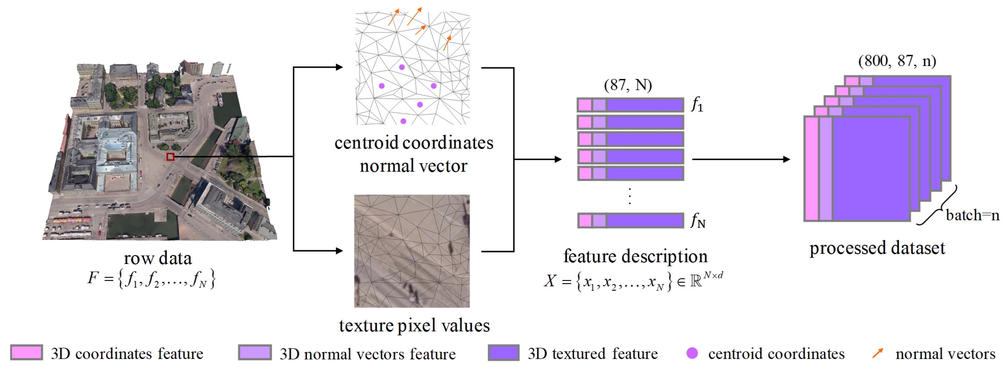
Feature Descriptors. Establishing a unified and comprehensive set of feature descriptors is crucial given the irregularity and complexity of 3D mesh scene data. Centroid coordinates capture the spatial position of each mesh, providing essential contextual information for understanding its location. Normal vectors offer crucial information about surface orientation, aiding in the understanding of geometric structure. Texture information provides rich appearance details, significantly enhancing the model’s ability to differentiate between different semantic categories. To effectively represent urban-scale environments, we combined normal vectors, centroid coordinates, and 27 texture pixel values to describe the spatial orientation and attributes of each sample. As analyzed in

Table 2. Impact of different input features on feature representation learning (%).

Model	OA	mAcc	mIoU	mF1
Ours	91.9	79.3	62.8	74.5
No Normal Vector	85.6	64.2	48.2	60.2
No Center Coordinate	87.2	67.0	51.5	63.8
No Textures	80.1	72.2	46.6	59.7

, different feature combinations impact downstream semantic segmentation performance, with texture information playing a pivotal role due to its rich attribute details. Additionally, normal vectors and centroid coordinates are essential for capturing spatial position and orientation. While we explored other feature descriptors, our evaluation confirmed that this combination best balances geometric and appearance information, making it well suited for urban 3D mesh representation.

Additionally, we observed that 3D meshes have other potential feature descriptors, such as curvature features and area features. When computing curvature features, we extracted the following curvature descriptors: principal curvatures ($k_1$, $k_2$), mean curvature (($k_1$ + $k_2$)/2), Gaussian curvature ($k_1$, $k_2$), and principal curvature directions ($d_1$, $d_2$). Subsequently, we constructed a curvature feature vector (30 dimensions) by concatenating the curvature features of the three vertices of each face. Furthermore, we also computed the area features of the 3D mesh (1 dimension). The results of the corresponding ablation experiments are shown in

Table 3. Impact of other input features on feature representation learning (%).

Model	OA	mAcc	mIoU	mF1
Ours	91.9	79.3	62.8	74.5
Add Curvature	89.6	76.3	57.3	72.0
Add Surface Area	91.0	79.0	60.4	72.3

.

In 3D-mesh-based urban scene datasets, curvature and triangular face area features are less effective due to several factors. Urban structures are predominantly flat, resulting in near-zero curvature with limited discriminative power. Variations in mesh resolution introduce noise, making curvature and area calculations less reliable. Additionally, face area is influenced by tessellation rather than intrinsic object properties, reducing its usefulness. In contrast, normal vectors and RGB textures offer more informative features, while deep learning techniques can automatically learn more robust representations. These geometric features may be more suitable for object part segmentation rather than large-scale urban scene segmentation.

(2) Network Branches

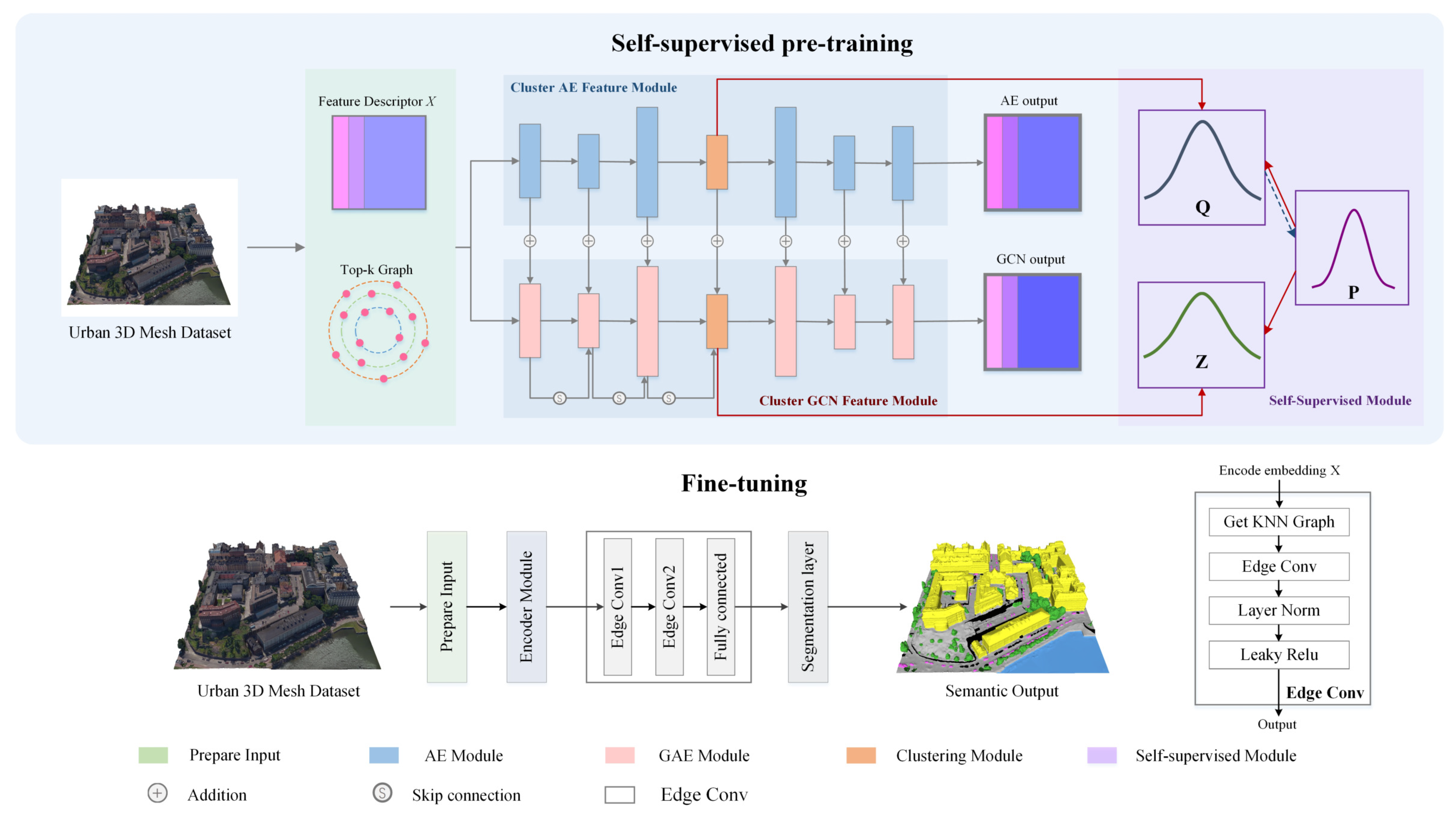
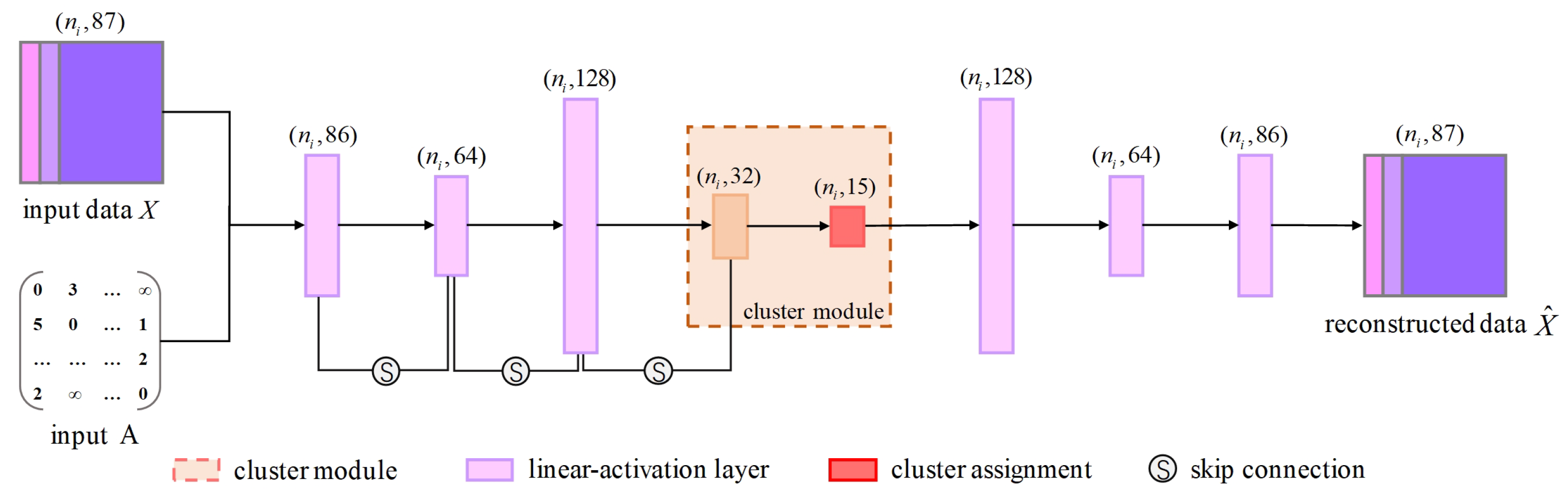
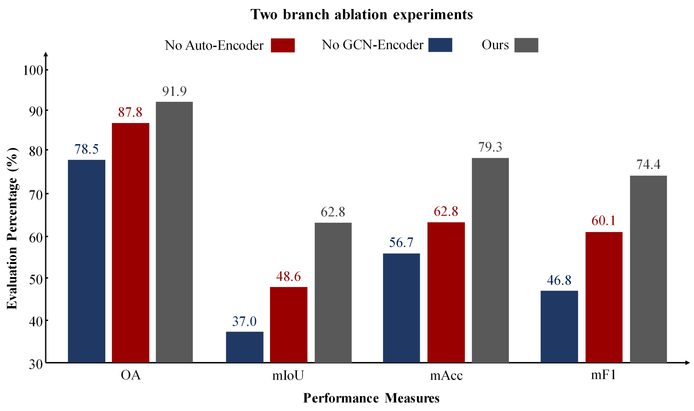
Dual-Branch Network. Our architecture combines an autoencoder and a graph encoder for representation learning. We conducted experiments to validate the effectiveness of each branch. We compared the performance of our dual-branch network with that of networks using only the autoencoder, only the graph encoder, and the fusion of both branches for feature representation in downstream semantic segmentation tasks. The results are shown in Figure 10.

The experimental results indicate that using only an autoencoder for clustering 3D mesh sample points fails to capture the structural relationships between the samples, while relying solely on a GCN leads to a lack of understanding of the data’s inherent feature attributes. Our approach, which integrates the encoded features from the autoencoder with the structural features from the GCN, achieves superior segmentation performance.

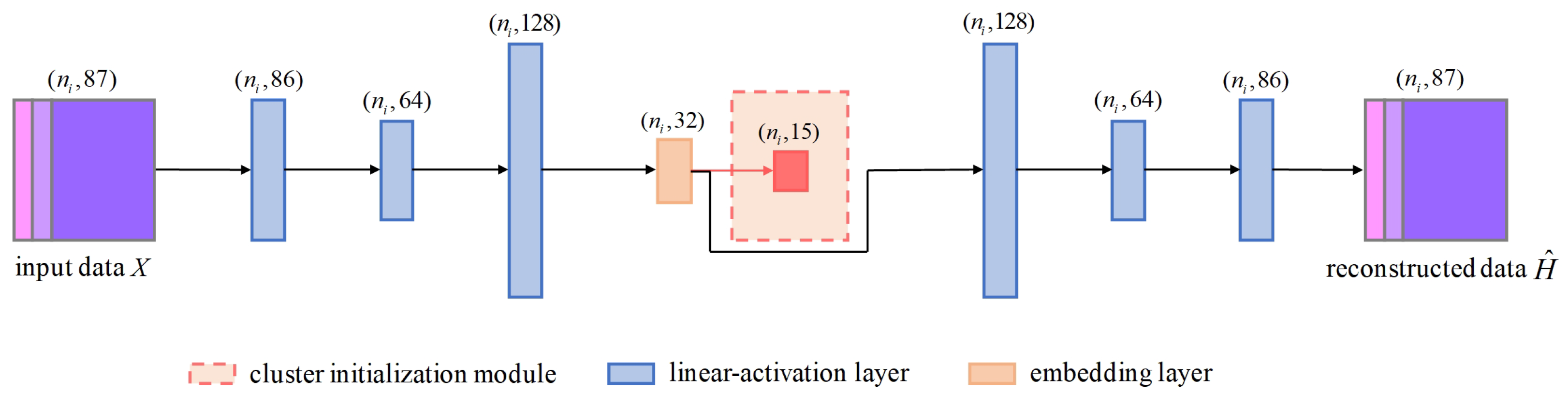
(3) Impact of Sample Size on Cluster Initialization

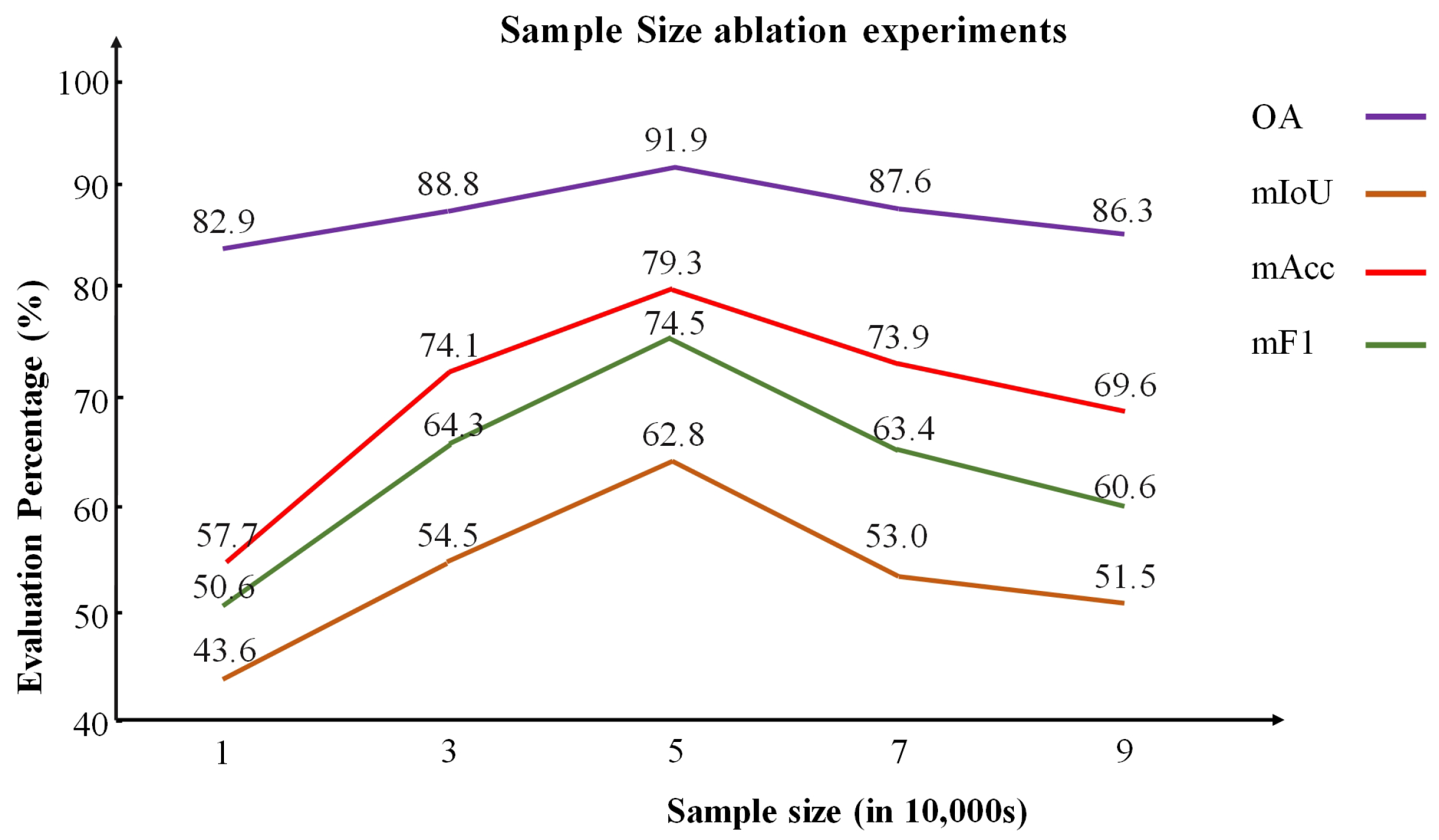
We validate the choice of selecting 50,000 points by analyzing how different numbers of initialized cluster center samples impact deep clustering and semantic segmentation performance (

Table 4. Time consumption for initializing cluster centers with different sample sizes (in seconds).

Sample Size (in 10,000 s)	1	3	5	7	9
Time Consumption (s)	2.4	6.5	10.8	14.7	19.5

). The sampled data have been preprocessed and stored in a specific file. As shown in Figure 11, using more samples provides broader coverage but increases computational and preprocessing time and is more prone to class imbalance. Conversely, using too few points fails to capture global features, reducing feature learning, while too many points introduce redundancy and affect performance. Sampling 50,000 points achieves the best balance between representativeness and efficiency, significantly enhancing semantic segmentation performance. This underscores the importance of balancing coverage and efficiency in sampling strategies.

We also compared different sampling strategies for cluster center initialization, as shown in

Table 5. Impact of different sampling methods on cluster center initialization (%).

Sampling Method	OA	mAcc	mIoU	mF1
FPS	91.9	79.3	62.8	74.5
RS	85.7	59.2	49.7	54.5
PGS	87.5	64.4	54.6	59.4

. The results show that FPS ensures more uniform coverage and better feature representativeness, while RS and PGS tend to bias towards regions with more samples, reducing clustering performance.

(4) Impact of Cluster Number on Feature Learning

Due to the complexity and diversity of urban 3D mesh scene datasets, the number of clusters cannot be directly equated to ground truth label categories [60]. To better capture the internal structure and details of 3D mesh data, we conducted experiments using different cluster numbers, as shown in

Table 6. Impact of different cluster count on feature representation learning (%).

Feature Clusters (n)	OA	mAcc	mIoU	mF1
6	82.3	65.3	41.2	51.0
9	85.8	77.1	52.6	65.1
12	90.7	76.3	57.8	68.4
15	91.9	79.3	62.8	74.5
18	91.0	77.1	59.1	70.4
21	90.7	77.8	57.7	69.5

.

Although we did not exhaustively test all possible cluster numbers, our observations indicate that when $k<12$, the number of clusters is insufficient to fully represent the semantic features of urban scenes, leading to a drop in model performance. Conversely, when $k>18$, the cluster number becomes redundant relative to the semantic features of the scene, causing a gradual performance decline. These results validate our hypothesis: for complex urban 3D mesh scenes, the number of clusters should not simply match the number of ground truth categories. Too few clusters can limit the performance of self-supervised representation learning. Therefore, we recommend setting the cluster number to 2 to 3 times the number of label categories, with 2.5 times being optimal, in deep clustering for semantic segmentation.

(5) Analysis of K-Nearest Neighbors in GCN

In the graph encoder branch, selecting an appropriate K-nearest neighbor (KNN) count is crucial for effectively capturing both local and global features in 3D mesh scene data. Experimental results indicate that when the K value is less than 7, the neighborhood information in the KNN graph is insufficient, limiting the network’s ability to learn local structures. Conversely, when the K value exceeds 10, excessive overlap occurs in the KNN graph, leading to information redundancy and degrading model performance.

Through extensive experiments, as shown in

Table 7. Impact of different numbers of K-neighbors in GCN branch of our model (%).

Nearest Neighbors (K)	OA	mAcc	mIoU	mF1
5	88.2	74.6	55.7	67.5
7	91.9	79.3	62.8	74.5
10	90.9	80.8	60.6	71.9
13	78.2	75.9	42.0	51.7

, we found that the model achieves optimal performance when the K value is set to 7, indicating that this value strikes the best balance between information aggregation and noise suppression within the local neighborhood. These findings highlight the sensitivity of graph convolutional networks to the choice of K-neighbors. Therefore, we recommend selecting a K value between 7 and 10 in practical applications to achieve optimal learning performance.

(6) Impact of Supervision Label Quantity

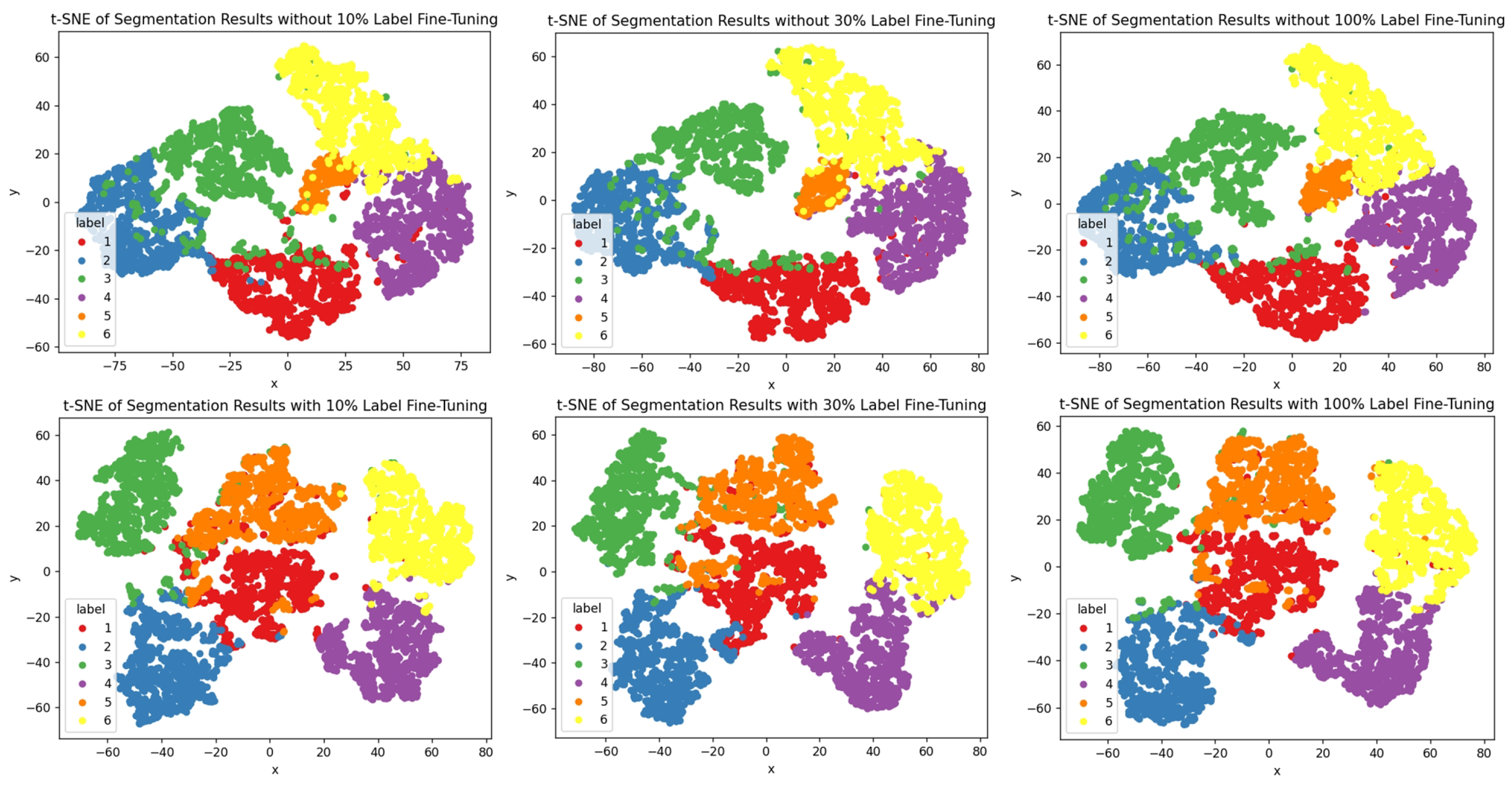
Under the self-supervised learning framework, we fine-tuned the network using 0.1%, 1%, 10%, 30%, and 100% of the labeled samples and compared their performance on downstream tasks. The experimental results shown in

Table 8. Impact of label proportion on downstream semantic segmentation performance (%).

Label Proportion (%)	OA	mAcc	mIoU	mF1
0.1	86.6	62.6	51.2	62.5
1	89.4	72.8	55.4	68.6
10	91.9	79.3	62.8	74.5
30	92.9	80.5	65.0	76.5
100	93.2	80.8	66.1	77.6

demonstrate that, even with only 10% of the labeled data, the network’s performance is nearly on par with that of using the full set of labeled data. This finding highlights the effectiveness and robustness of our self-supervised approach in feature learning, showing that it can achieve accuracy comparable to fully supervised models, even in scenarios with limited labels. Furthermore, when using only 0.1% and 1% of labeled samples, the accuracy slightly decreases due to sample imbalance; however, our method still outperforms existing approaches in comparative experiments. The specific details of the comparative experiments will be introduced in Section 4.6. 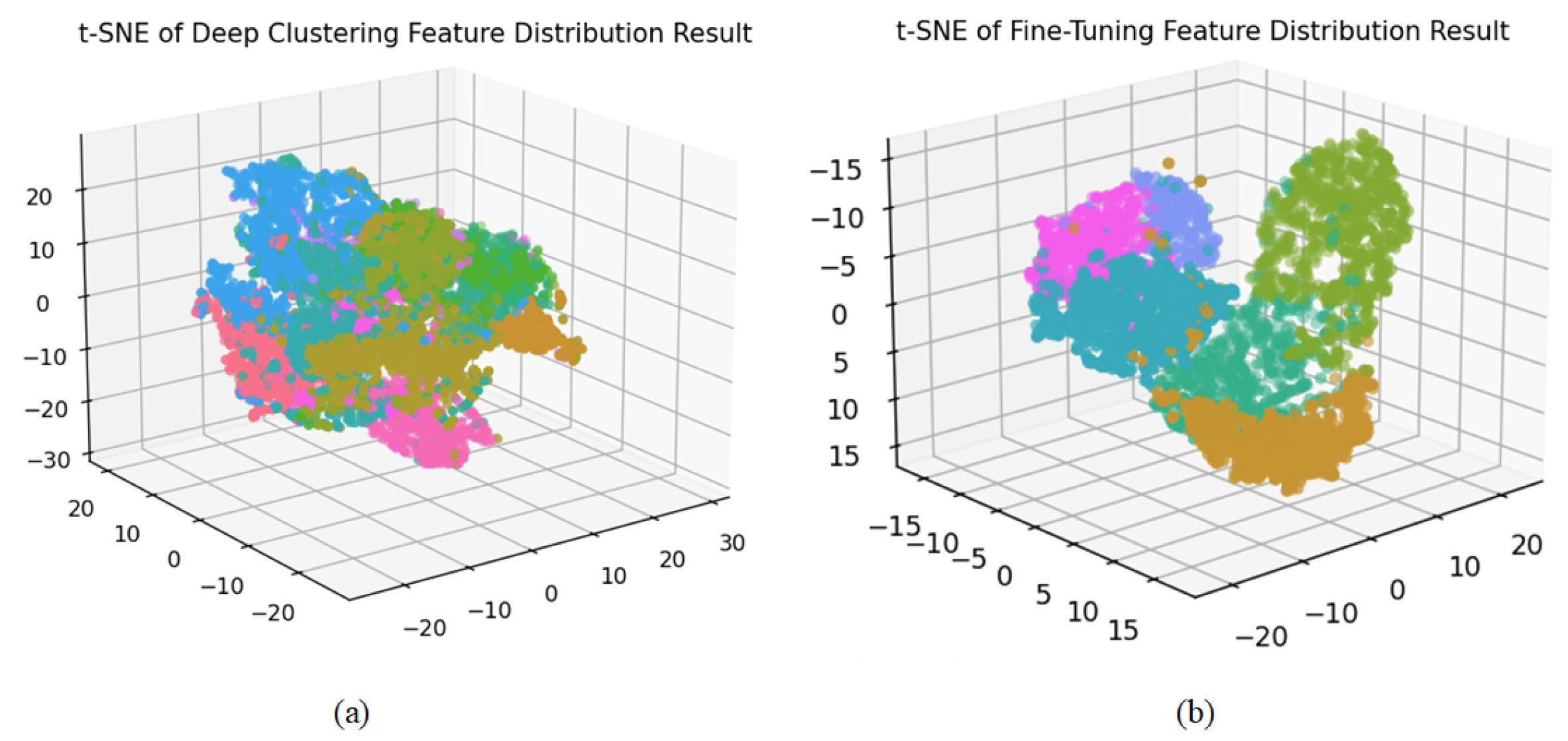Figure 12 visualizes the cluster distribution [61], where we observe similar patterns, further validating the effectiveness of our pre-trained network in feature representation.

(7) Impact of Sample Selection Strategy in Fine-Tuning

As shown in

Table 9. Impact of different fine-tuning strategy on downstream semantic segmentation performance (%).

Fine-Tuning Strategy	OA	mAcc	mIoU	mF1
Subset Fine-Tuning	91.9	79.3	62.8	74.5
In-Batch Samples Fine-Tuning	91.8	80.2	63.3	74.8

, we explored two fine-tuning strategies, with our 10% label samples selected only once at the beginning and fixed for all subsequent training epochs.

Subset Fine-Tuning Strategy. In this approach, the urban 3D mesh is first divided into batches. Then, 10% of these batches are randomly selected for fine-tuning, while the remaining 90% of the batches are skipped. This method emphasizes focusing the fine-tuning process on a smaller, randomly selected subset of the data, thereby optimizing model performance. This subset selection strategy ensures effective training on a relatively limited amount of data while reducing computational resource consumption.

In-Batch Sample Fine-Tuning Strategy. In this strategy, 10% of the samples within each batch are randomly selected for loss calculation, while the remaining 90% of the samples in the batch are excluded from loss computation. This method allows the model to process the entire urban 3D mesh while learning from only a small subset of samples in each batch.

We conducted a comprehensive evaluation of two fine-tuning strategies. The experimental results indicate that there is no significant difference in test accuracy between the two strategies. However, the subset fine-tuning strategy significantly reduces time consumption, with training time approximately ${\displaystyle \frac{1}{10}}$th that of the in-batch sample fine-tuning strategy. By randomly selecting batches of samples, the subset fine-tuning strategy minimizes training variability and human intervention, thereby enhancing robustness on large-scale scene datasets. We performed ten downstream task experiments, and the results showed that the distribution of labels in the subset fine-tuning remained consistent with the test set, and the test accuracy was relatively stable. However, it is important to note that the effectiveness of this strategy depends on the quality of feature representation learning in the pre-training task. If the pre-training task performs poorly, fine-tuning results may exhibit higher variance, leading to instability in test accuracy.

4.6. Evaluation of Competition Methods

Due to the lack of self-supervised models in urban 3D mesh segmentation, we mainly evaluated SCRM-Net by comparing it with competitive supervised models under the same training conditions to demonstrate its robustness in representation learning. We evaluated five strong baseline models for urban 3D mesh scene semantic segmentation on the SUM urban 3D mesh: PointNet [62], PointNet++ [42], dynamic graph convolutional network (DGCNN) [5], kernel point convolution (KPConv) [10], and SUM [15]. To mitigate random factors, each model was tested in ten independent experiments, with the average results reported. Additionally, we analyzed model accuracy under both 10% and 100% labeled data settings for a comprehensive performance evaluation, as shown in

Table 10. Accuracy comparisons among different methods. The results reported in this table are IOU (%) of each class, OA (%), mAcc (%), mIoU (%), and mF1 (%).

	Label Proportion	Ground	Vegetation	Building	Water	Car	Boat	OA	mAcc	mIoU	mF1
Ours	0.1%	40.5	81.4	77.8	48.8	28.0	30.7	86.6	62.6	51.2	62.5
	1%	41.0	83.8	87.8	52.2	32.5	35.1	89.4	72.8	55.4	68.6
	10%	72.4	89.2	91.9	54.3	30.4	38.7	91.9	79.3	62.8	74.5
SQN [63]	0.1%	57.3	62.7	67.2	35.5	15.7	17.8	81.0	59.3	42.7	53.0
	1%	62.6	67.6	74.3	44.2	19.8	21.3	83.8	60.7	48.3	56.3
	10%	64.1	73.2	77.7	46.3	21.0	24.9	86.5	62.2	51.2	59.0
PointNet [62]	10%	30.5	44.0	51.7	1.3	1.5	0.0	59.3	33.0	21.5	30.3
	100%	64.0	56.5	63.6	4.2	19.2	2.4	72.5	65.5	35.0	45.5
PointNet++ [42]	10%	37.0	55.4	54.5	0.2	1.4	0.0	63.6	36.6	24.7	33.2
	100%	62.5	70.4	76.6	4.0	18.1	1.8	80.0	67.2	38.9	48.0
DGCNN [5]	10%	56.3	81.0	70.1	23.9	0.0	1.5	75.6	66.6	38.8	47.6
	100%	64.4	84.5	87.1	36.6	22.9	19.9	87.6	61.3	52.6	64.5
KPConv [10]	10%	68.1	54.2	65.9	54.3	11.1	5.9	77.1	56.8	43.2	55.4
	100%	86.5	88.4	92.7	77.7	54.3	13.3	93.3	73.3	68.8	76.7
SUM [15]	10%	59.3	66.1	65.8	52.4	10.1	2.3	76.3	55.7	42.7	52.0
	100%	83.3	90.5	92.5	86.0	37.3	7.4	93.0	70.6	66.2	73.8

.

We further evaluated two representative self-supervised learning models: SQN [63] and MeshMAE [64]. Experimental results indicate that MeshMAE is suitable for small-scale, closed 3D mesh surface data. However, in large-scale urban scenarios, the dataset simplification during preprocessing leads to blurred boundaries for fine-grained semantic categories (e.g., water, cars, and boats), significantly degrading the segmentation performance. As the results were not meaningful, they are not presented. Simultaneously, we tested the SQN model on the SUM dataset, and the results revealed that traditional point-cloud-based semantic segmentation frameworks perform poorly on complex mesh structures. We attribute this performance degradation primarily to the inherent inconsistency between point cloud representations and mesh structures, with the former being unable to fully capture and leverage the rich topological and geometric information embedded in mesh surfaces. These comparative results further highlight the importance and necessity of developing specialized models tailored for mesh structures.

As shown in Table 10, the results indicate that SCRM-Net achieves strong performance in self-supervised representation learning, even on complex urban 3D mesh datasets. Unlike supervised methods that require large amounts of labeled data, SCRM-Net only needs 10% of randomly selected labels for fine-tuning to achieve competitive segmentation accuracy. Furthermore, our method does not require careful selection of fine-tuning labels, reducing annotation costs and showing good adaptability. In contrast, supervised models suffer a significant drop in accuracy without large-scale labeled samples.

Although some of the supervised learning methods listed in the table outperform our model under fully supervised conditions, when using only 10% of the sample labels, SCRM-Net’s performance far exceeds that of the other supervised methods. Specifically, compared to the other five proposed methods, SCRM-Net achieves a range from 12.7 to 46.3% in mAcc, from 17.7 to 39.4% in mIoU, and from 19.0 to 44.1% in mF1. This demonstrates that our proposed model, with its simple yet effective network structure, can achieve competitive semantic segmentation results on textured 3D mesh.

4.7. Generalization Ability

To evaluate the applicability of SCRM-Net across different datasets, we conducted an experiment to assess its generalization ability. The H3D dataset, a textured and labeled 3D mesh of Hessigheim village in Germany, shares similarities with the SUM dataset as both represent urban scenes with imbalanced label distributions, making it a suitable benchmark for generalization testing. However, despite their similarities, the two datasets differ in category definitions. To ensure consistency, we merged and remapped the H3D categories to align with the SUM dataset, unifying them into four typical urban scene classes: terrain (including low vegetation, urban furniture, impervious surface, soil/gravel), high vegetation (shrub and tree), buildings (roof, facade, chimney and vertical surface), and vehicles. To evaluate generalization, we compared our method with PSS-Net [45], and the detailed results are presented in

Table 11. Accuracy comparisons among different datasets. The results reported in this table are IoU (%) of each class and mIoU (%).

	Label Proportion	Ground	Vegetation	Building	Vehicles	mIoU
Ours	10%	55.2	57.2	51.5	16.7	45.1
	100%	66.7	64.0	49.8	17.6	49.5
PSS-Net [45]	10%	40.4	50.2	35.0	8.0	33.4
	100%	74.2	66.2	44.5	13.4	49.6

. Since it relies on supervised learning, we trained it with only 10% of labeled data to simulate a low-annotation scenario and ensure a fair comparison.

In our experiments, we first trained SCRM-Net on the SUM dataset (using 12 training tiles from Section 4.1) and then fine-tuned and evaluated it on the H3D test set. During fine-tuning, we removed the weighted cross-entropy loss to improve adaptability to different class distributions while still randomly selecting 10% of the samples to fine-tune the network. The results demonstrate that SCRM-Net maintains strong performance on H3D, indicating its generalization ability across 3D mesh datasets with similar scene characteristics. Furthermore, the comparative experiments in Section 4.6 show that our self-supervised deep clustering representation learning effectively captures the intrinsic features of urban scenes, enhancing robustness to variations in data distribution.

4.8. Visualization of Feature Learning Results

This subsection presents the visualization experiments of SCRM-Net during the feature learning and fine-tuning stages to evaluate its performance in feature learning. Specifically, we employ the t-SNE visualization technique to project the deep clustering features extracted from the pretext task and the fine-tuned features into 3D space. As shown in Figure 13, SCRM-Net achieves good inter-cluster separability during the deep clustering learning stage, with fewer ambiguous samples. In the fine-tuning stage, after adding 10% of labeled data for fine-tuning, the cluster boundaries become more distinct, further validating the effectiveness of the proposed method.

5. Further Analysis

5.1. Error Analysis

We further analyzed the misclassification patterns of SCRM-Net, as illustrated in Figure 14. Here, we summarize the key issues. 1. Category Confusion: Misclassification often occurs between visually or structurally similar categories, such as low-rise buildings misclassified as ground (f) and artificial ponds mistaken for roads (e). 2. Labeling Errors: As shown in (b) and (c), mislabeled ground truth introduces noise during training, such as trees being labeled as buildings or ground mislabeled as water, affecting the model’s ability to learn accurate features. 3. Environmental Interference: As seen in (a), factors like building shadows and reflective surfaces (e.g., car windows) can cause vehicles to be misclassified as ground. 4. Class Imbalance: Underrepresented categories (e.g., boats and cars) suffer from higher misclassification rates, likely due to limited samples during fine-tuning. 5. Texture Complexity Noise: Categories with intricate textures or noise-prone surfaces are more susceptible to errors. For example, as shown in (d), noise in boat textures leads to incorrect classification.

These misclassification regions highlight the key challenges faced by SCRM-Net in semantic segmentation. Ablation experiments on feature descriptors demonstrate that texture features are the most critical factors influencing model performance. In the future, additional preprocessing methods, including shadow removal and reflection compensation, could help mitigate the impact of lighting and shadows on texture features. Furthermore, the use of texture denoising techniques or texture-aware feature learning could enhance the model’s robustness in complex textured environments.

5.2. Noise Robustness Analysis

To evaluate the robustness of SCRM-Net in real-world complex environments, we introduced varying levels of noise and missing data in our dataset, as shown in

Table 12. Impact of different noise disturbances on semantic segmentation performance (%).

Data Perturbation	Setting	OA	mAcc	mIoU	mF1
Gaussian Noise	$\sigma$ = 0.01	91.4	77.9	60.8	70.9
	$\sigma$ = 0.05	90.3	70.0	58.9	69.1
Random Masking	mask = 10%	92.0	79.1	62.5	75.0
	mask = 30%	91.6	77.6	61.7	73.9

.

• Gaussian Noise Interference: We add two levels of Gaussian noise to assess SCRM-Net’s robustness: 0.01 for minor sensor errors and 0.05 for extreme disturbances. The model maintains high accuracy under low noise but shows degraded performance with increased noise, leading to higher misclassification in cars and boats. Nonetheless, it maintains overall classification ability, indicating a certain level of noise resistance.
• Random Masking: To evaluate SCRM-Net’s robustness to missing data, we randomly masked 10% and 30% of the data rows by setting their feature values to zero. Results show that 10% masking has minimal impact on model performance, while 30% masking causes a slight decline in semantic segmentation accuracy, particularly in small sample categories. Nonetheless, overall classification ability remains stable, indicating strong robustness to missing data.

6. Conclusions

Although 3D mesh semantic segmentation has become a popular research direction in recent years, to the best of our knowledge, this is the first study to apply self-supervised deep clustering methods to learn semantic representations for 3D mesh. We propose a balanced sampling strategy based on FPS for initializing cluster centers and utilize an improved dual-branch encoding architecture to achieve robust feature encoding for urban 3D mesh. For the semantic segmentation task, we randomly selected 10% of the ground truth labels for fine-tuning and achieved state-of-the-art segmentation results on a six-class urban 3D mesh, with overall accuracy (OA), mean precision (mP), mean recall (mR), mean F1 score (mF1), and mean intersection over union (mIoU) of 91.9%, 71.4%, 79.3%, 74.5%, 62.8%, respectively. Experimental results demonstrate that SCRM-Net can effectively represent features of urban 3D mesh scene datasets.

Furthermore, urban 3D mesh scene datasets commonly suffer from class imbalance issues, which present challenges for learning robust semantic representations under self-supervised settings—particularly for underrepresented classes. Addressing this widespread issue will be a key focus of our future work. In addition, we plan to extend our method to more diverse types of 3D data, including industrial and natural environment datasets, to further enhance the model’s representation ability and adaptability across a broader range of real-world scenarios.

References

1. Hernández, L.; Hernández, S. Application of digital 3D models on urban planning and highway design. WIT Trans. Built Environ. 1997, 33, 12. [Google Scholar]
2. Yang, X. Urban Remote Sensing: Monitoring, Synthesis and Modeling in the Urban Environment. 2011. Available online: https://searchworks.stanford.edu/view/12262036 (accessed on 16 January 2025).
3. Kaul, M.; Yang, B.; Jensen, C.S. Building accurate 3D spatial networks to enable next generation intelligent transportation systems. In Proceedings of the 2013 IEEE 14th International Conference on Mobile Data Management, Milan, Italy, 3–6 June 2013; Voulme 1, pp. 137–146. [Google Scholar]
4. Salah, I.B.; Kramm, S.; Demonceaux, C.; Vasseur, P. Summarizing large scale 3D mesh for urban navigation. Robotics Auton. Syst. 2022, 152, 104037. [Google Scholar] [CrossRef]
5. Thomas, H.; Qi, C.; Deschaud, J.-E.; Marcotegui, B.; Goulette, F.; Guibas, L.J. KPConv: Flexible and deformable convolution for point clouds. In Proceedings of the 2019 IEEE/CVF International Conference on Computer Vision (ICCV), Seoul, Republic of Korea, 27 October–2 November 2019; pp. 6410–6419. [Google Scholar]
6. Landrieu, L.; Simonovsky, M. Large-scale point cloud semantic segmentation with superpoint graphs. In Proceedings of the 2018 IEEE/CVF Conference on Computer Vision and Pattern Recognition, Honolulu, HI, USA, 21–26 July 2017; pp. 4558–4567. [Google Scholar]
7. Hu, Q.; Yang, B.; Xie, L.; Rosa, S.; Guo, Y.; Wang, Z.; Trigoni, A.; Markham, A. RandLA-Net: Efficient semantic segmentation of large-scale point clouds. In Proceedings of the 2020 IEEE/CVF Conference on Computer Vision and Pattern Recognition (CVPR), Seattle, WA, USA, 13–19 June 2019; pp. 11105–11114. [Google Scholar]
8. Nguyen, A.V.; Le, H.B. 3D point cloud segmentation: A survey. In Proceedings of the 2013 6th IEEE Conference on Robotics, Automation and Mechatronics (RAM), Manila, Philippines, 12–15 November 2013; pp. 225–230. [Google Scholar]
9. Gao, L.; Liu, Y.; Liu, Y.; Cheng, X.; Zhu, J.; Wang, J. Large-scale 3D mesh data semantic segmentation: A survey. In Proceedings of the 2023 9th International Conference on Big Data and Information Analytics (BigDIA), Haikou, China, 15–17 December 2023; pp. 81–89. [Google Scholar]
10. Zhang, R.; Zhang, G.; Yin, J.; Jia, X.; Mian, A.S. Mesh-based DGCNN: Semantic segmentation of textured 3-D urban scenes. IEEE Trans. Geosci. Remote Sens. 2023, 61, 4402812. [Google Scholar] [CrossRef]
11. Rouhani, M.; Lafarge, F.; Alliez, P. Semantic segmentation of 3D textured meshes for urban scene analysis. ISPRS J. Photogramm. Remote Sens. 2017, 123, 124–139. [Google Scholar] [CrossRef]
12. Jing, L.; Tian, Y. Self-supervised visual feature learning with deep neural networks: A survey. IEEE Trans. Pattern Anal. Mach. Intell. 2019, 43, 4037–4058. [Google Scholar] [CrossRef]
13. Balestriero, R.; Ibrahim, M.; Sobal, V.; Morcos, A.S.; Shekhar, S.; Goldstein, T.; Bordes, F.; Bardes, A.; Mialon, G.; Tian, Y.; et al. A cookbook of self-supervised learning. arXiv 2023, arXiv:abs/2304.12210. [Google Scholar]
14. Ren, Y.; Pu, J.; Yang, Z.; Xu, J.; Li, G.; Pu, X.; Yu, P.S.; He, L. Deep clustering: A comprehensive survey. IEEE Trans. Neural Netw. Learn. Syst. 2022, 36, 5858–5878. [Google Scholar] [CrossRef]
15. Gao, W.; Nan, L.; Boom, B.; Ledoux, H. SUM: A benchmark dataset of semantic urban meshes. arXiv 2021, arXiv:abs/2103.00355. [Google Scholar] [CrossRef]
16. Hershey, J.R.; Chen, Z.; Le Roux, J.; Watanabe, S. Deep clustering: Discriminative embeddings for segmentation and separation. In Proceedings of the 2016 IEEE International Conference on Acoustics, Speech and Signal Processing (ICASSP), Shanghai, China, 20–25 March 2016; pp. 31–35. [Google Scholar]
17. Zhou, S.; Xu, H.; Zheng, Z.; Chen, J.; Li, Z.; Bu, J.; Wu, J.; Wang, X.; Zhu, W.; Ester, M. A comprehensive survey on deep clustering: Taxonomy, challenges, and future directions. arXiv 2022, arXiv:abs/2206.07579. [Google Scholar] [CrossRef]
18. Caron, M.; Bojanowski, P.; Joulin, A.; Douze, M. Deep clustering for unsupervised learning of visual features. In Proceedings of the European Conference on Computer Vision, Munich, Germany, 8–14 September 2018. [Google Scholar]
19. Jabi, M.; Pedersoli, M.; Mitiche, A.; Ayed, I.B. Deep clustering: On the link between discriminative models and K-means. IEEE Trans. Pattern Anal. Mach. Intell. 2018, 43, 1887–1896. [Google Scholar] [CrossRef]
20. Hinton, G.E.; Salakhutdinov, R.R. Reducing the dimensionality of data with neural networks. Science 2006, 313, 504–507. [Google Scholar] [CrossRef] [PubMed]
21. Yang, B.; Fu, X.; Sidiropoulos, N.; Hong, M. Towards K-means-friendly spaces: Simultaneous deep learning and clustering. In Proceedings of the International Conference on Machine Learning, Sydney, NSW, Australia, 6–11 August 2016. [Google Scholar]
22. Li, G.; Müller, M.; Thabet, A.K.; Ghanem, B. DeepGCN: Can GCN be more general? In Proceedings of the 2020 IEEE/CVF Conference on Computer Vision and Pattern Recognition (CVPR), Seattle, WA, USA, 13–19 June 2020; pp. 9397–9406. [Google Scholar]
23. Gui, J.; Chen, T.; Zhang, J.; Cao, Q.; Sun, Z.; Luo, H.; Tao, D. A Survey on Self-Supervised Learning: Algorithms, Applications, and Future Trends. IEEE Trans. Pattern Anal. Mach. Intell. 2024, 46, 9052–9071. [Google Scholar] [CrossRef] [PubMed]
24. Ran, L.; Li, Y.; Liang, G.; Zhang, Y. Pseudo Labeling Methods for Semi-Supervised Semantic Segmentation: A Review and Future Perspectives. IEEE Trans. Circuits Syst. Video Technol. 2024, 35, 3054–3080. [Google Scholar] [CrossRef]
25. Bengio, Y.; Courville, A.C.; Vincent, P. Representation Learning: A Review and New Perspectives. IEEE Trans. Pattern Anal. Mach. Intell. 2012, 35, 1798–1828. [Google Scholar] [CrossRef]
26. Xie, J.; Girshick, R.B.; Farhadi, A. Unsupervised Deep Embedding for Clustering Analysis. arXiv 2015, arXiv:abs/1511.06335. [Google Scholar]
27. Guo, X.; Gao, L.; Liu, X.; Yin, J. Improved Deep Embedded Clustering with Local Structure Preservation. In Proceedings of the International Joint Conference on Artificial Intelligence, Melbourne, VIC, Australia, 19–25 August 2017. [Google Scholar]
28. Khan, M.R.; Blumenstock, J.E. Multi-GCN: Graph Convolutional Networks for Multi-View Networks, with Applications to Global Poverty. In Proceedings of the AAAI Conference on Artificial Intelligence, Honolulu, HI, USA, 27 January–1 February 2019. [Google Scholar]
29. Chung, F.R.; Graham, F.C. Spectral Graph Theory; American Mathematical Society: Providence, RI, USA, 1997. [Google Scholar]
30. Kipf, T.; Welling, M. Variational Graph Auto-Encoders. arXiv 2016, arXiv:abs/1611.07308. [Google Scholar]
31. Wang, C.; Pan, S.; Hu, R.; Long, G.; Jiang, J.; Zhang, C. Attributed Graph Clustering: A Deep Attentional Embedding Approach. In Proceedings of the International Joint Conference on Artificial Intelligence, Macao, China, 10–16 August 2019. [Google Scholar]
32. Bo, D.; Wang, X.; Shi, C.; Zhu, M.; Lu, E.; Cui, P. Structural Deep Clustering Network. In Proceedings of the Web Conference 2020, Taipei, China, 20–24 April 2020. [Google Scholar]
33. Jiao, X.; Chen, Y.; Yang, X. SCMS-Net: Self-Supervised Clustering-Based 3D Meshes Segmentation Network. Comput. Aided Des. 2023, 160, 103512. [Google Scholar] [CrossRef]
34. Adam, J.M.; Liu, W.; Zang, Y.; Afzal, M.K.; Bello, S.A.; Muhammad, A.U.; Wang, C.; Li, J. Deep learning-based semantic segmentation of urban-scale 3D meshes in remote sensing: A survey. Int. J. Appl. Earth Obs. Geoinf. 2023, 121, 103365. [Google Scholar] [CrossRef]
35. He, Y.; Yu, H.; Liu, X.-Y.; Yang, Z.; Sun, W.; Wang, Y.; Fu, Q.; Zou, Y.; Mian, A.S. Deep Learning based 3D Segmentation: A Survey. arXiv 2021, arXiv:abs/2103.05423. [Google Scholar]
36. Ray, N.; Li, W.-C.; Lévy, B.; Sheffer, A.; Alliez, P. Periodic global parameterization. ACM Trans. Graph. 2006, 25, 1460–1485. [Google Scholar] [CrossRef]
37. Li, S.; Luo, Z.; Zhen, M.; Yao, Y.; Shen, T.; Fang, T.; Quan, L. Cross-Atlas Convolution for Parameterization Invariant Learning on Textured Mesh Surface. In Proceedings of the 2019 IEEE/CVF Conference on Computer Vision and Pattern Recognition (CVPR), Long Beach, CA, USA, 15–20 June 2019; pp. 6136–6145. [Google Scholar]
38. Huang, J.; Zhou, Y.; Nießner, M.; Shewchuk, J.R.; Guibas, L.J. QuadriFlow: A Scalable and Robust Method for Quadrangulation. Comput. Graph. Forum 2018, 37, 147–160. [Google Scholar] [CrossRef]
39. Huang, J.; Zhang, H.; Yi, L.; Funkhouser, T.A.; Nießner, M.; Guibas, L.J. TextureNet: Consistent Local Parametrizations for Learning from High-Resolution Signals on Meshes. In Proceedings of the 2019 IEEE/CVF Conference on Computer Vision and Pattern Recognition (CVPR), Long Beach, CA, USA, 15–20 June 2019; pp. 4435–4444. [Google Scholar]
40. Chen, J.; Xu, Y.; Lu, S.; Liang, R.; Nan, L. 3D Instance Segmentation of MVS Buildings. IEEE Trans. Geosci. Remote Sens. 2021, 60, 5704014. [Google Scholar]
41. Grzeczkowicz, G.; Vallet, B. Semantic Segmentation of Urban Textured Meshes Through Point Sampling. arXiv 2022, arXiv:abs/2302.10635. [Google Scholar] [CrossRef]
42. Qi, C.; Yi, L.; Su, H.; Guibas, L.J. PointNet++: Deep Hierarchical Feature Learning on Point Sets in a Metric Space. arXiv 2017, arXiv:abs/1706.02413. [Google Scholar]
43. Tang, R.; Xia, M.; Yang, Y.; Zhang, C. A deep-learning model for semantic segmentation of meshes from UAV oblique images. Int. J. Remote Sens. 2022, 43, 4774–4792. [Google Scholar] [CrossRef]
44. Schult, J.; Engelmann, F.; Kontogianni, T.; Leibe, B. DualConvMesh-Net: Joint Geodesic and Euclidean Convolutions on 3D Meshes. In Proceedings of the 2020 IEEE/CVF Conference on Computer Vision and Pattern Recognition (CVPR), Seattle, WA, USA, 13–19 June 2020; pp. 8609–8619. [Google Scholar]
45. Gao, W.; Nan, L.; Boom, B.; Ledoux, H. PSSNet: Planarity-sensible Semantic Segmentation of Large-scale Urban Meshes. arXiv 2022, arXiv:abs/2202.03209. [Google Scholar] [CrossRef]
46. Liu, T.; Zhu, H.; Wei, Y.; Wei, S.; Zhao, Y.; Zhang, Y. Toward Accurate Human Parsing Through Edge Guided Diffusion. IEEE Trans. Image Process. 2024, 33, 2530–2543. [Google Scholar] [CrossRef]
47. Yang, Y.; Tang, R.; Xia, M.; Zhang, C. A surface graph based deep learning framework for large-scale urban mesh semantic segmentation. Int. J. Appl. Earth Obs. Geoinf. 2023, 119, 103322. [Google Scholar] [CrossRef]
48. Lei, H.; Akhtar, N.; Mian, A.S. Picasso: A CUDA-based Library for Deep Learning over 3D Meshes. In Proceedings of the 2021 IEEE/CVF Conference on Computer Vision and Pattern Recognition (CVPR), Nashville, TN, USA, 20–25 June 2021; pp. 13849–13859. [Google Scholar]
49. Lei, H.; Akhtar, N.; Shah, M.; Mian, A.S. Geometric Feature Learning for 3D Meshes. arXiv 2021, arXiv:abs/2112.01801. [Google Scholar]
50. Knott, M.; Groenendijk, R. Towards Mesh-Based Deep Learning for Semantic Segmentation in Photogrammetry. 2021. Available online: https://isprs-annals.copernicus.org/articles/V-2-2021/59/2021/ (accessed on 16 January 2025).
51. Zi, W.; Li, J.; Chen, H.; Chen, L.; Du, C. UrbanSegNet: An urban meshes semantic segmentation network using diffusion perceptron and vertex spatial attention. Int. J. Appl. Earth Obs. Geoinf. 2024, 129, 103841. [Google Scholar] [CrossRef]
52. Chen, T.; Kornblith, S.; Norouzi, M.; Hinton, G. A simple framework for contrastive learning of visual representations. In Proceedings of the 37th International Conference on Machine Learning, Online, 13–18 July 2020; p. 149. [Google Scholar]
53. Goodfellow, I.J.; Pouget-Abadie, J.; Mirza, M.; Xu, B.; Warde-Farley, D.; Ozair, S.; Courville, A.; Bengio, Y. Generative adversarial nets. In Proceedings of the 28th International Conference on Neural Information Processing Systems—Volume 2, Montreal, QC, Canada, 8–13 December 2014; pp. 2672–2680. [Google Scholar]
54. He, K.; Chen, X.; Xie, S.; Li, Y.; Dollár, P.; Girshick, R. Masked Autoencoders Are Scalable Vision Learners. In Proceedings of the 2022 IEEE/CVF Conference on Computer Vision and Pattern Recognition (CVPR), New Orleans, LA, USA, 18–24 June 2022; pp. 15979–15988. [Google Scholar]
55. Sohn, K.; Berthelot, D.; Li, C.L.; Zhang, Z.; Carlini, N.; Cubuk, E.D.; Kurakin, A.; Zhang, H.; Raffel, C. FixMatch: Simplifying Semi-Supervised Learning with Consistency and Confidence. Adv. Neural Inf. Process. Syst. 2020, 33, 596–608. [Google Scholar]
56. Zhu, L.; Shen, S.; Gao, X.; Hu, Z. Large Scale Urban Scene Modeling from MVS Meshes. In Proceedings of the Computer Vision—ECCV 2018, Munich, Germany, 8–14 September 2018; pp. 640–655. [Google Scholar]
57. Verdie, Y.; Lafarge, F.; Alliez, P. LOD Generation for Urban Scenes. ACM Trans. Graph. 2015, 34, 30. [Google Scholar] [CrossRef]
58. Arthur, D.; Vassilvitskii, S. k-means++: The advantages of careful seeding. In Proceedings of the ACM-SIAM Symposium on Discrete Algorithms, New Orleans, LA, USA, 7–9 January 2007. [Google Scholar]
59. Paszke, A.; Gross, S.; Massa, F.; Lerer, A.; Bradbury, J.; Chanan, G.; Killeen, T.; Lin, Z.; Gimelshein, N.; Antiga, L.; et al. PyTorch: An Imperative Style, High-Performance Deep Learning Library. arXiv 2019, arXiv:abs/1912.01703. [Google Scholar]
60. Yang, J.; Parikh, D.; Batra, D. Joint Unsupervised Learning of Deep Representations and Image Clusters. In Proceedings of the 2016 IEEE Conference on Computer Vision and Pattern Recognition (CVPR), Las Vegas, NV, USA, 27–30 June 2016; pp. 5147–5156. [Google Scholar]
61. Maaten, L.v.d.; Hinton, G.E. Visualizing Data using t-SNE. J. Mach. Learn. Res. 2008, 9, 2579–2605. [Google Scholar]
62. Qi, C.; Su, H.; Mo, K.; Guibas, L.J. PointNet: Deep Learning on Point Sets for 3D Classification and Segmentation. In Proceedings of the 2017 IEEE Conference on Computer Vision and Pattern Recognition (CVPR), Honolulu, HI, USA, 21–26 July 2017; pp. 77–85. [Google Scholar] [CrossRef]
63. Hu, Q.; Yang, B.; Fang, G.; Guo, Y.; Leonardis, A.; Trigoni, N.; Markham, A. SQN: Weakly-Supervised Semantic Segmentation of Large-Scale 3D Point Clouds; Springer: Cham, Switzerland, 2022; pp. 600–619. [Google Scholar]
64. Liang, Y.; Zhao, S.; Yu, B.; Zhang, J.; He, F. MeshMAE: Masked Autoencoders for 3D Mesh Data Analysis. arXiv 2022, arXiv:abs/2207.10228. [Google Scholar] [CrossRef]
Figure 1. Main framework of the proposed SCRM-Net (self-supervised deep clustering feature representation for urban 3D mesh semantic segmentation). The black arrows represent the input feature flow, while the red arrows illustrate the progressive alignment of the self-supervised module’s feature distribution with the standard distribution.
Remotesensing 17 01424 g001
Figure 2. Centroid coordinates, normal vectors, and 3D mesh textures are extracted to generate 3D mesh feature descriptors as general input for SCRM-Net. Then, we preprocess n 3D mesh samples into a tensor of shape (800, 87, n).
Remotesensing 17 01424 g002
Figure 3. A local example of FPS sampling based on feature descriptors. Initially, a random point is selected (red). The distance between the remaining points (blue) and the selected point is computed, and the point with the farthest distance is chosen as the second point. The process repeats by calculating the distance between the remaining points and the already selected points, selecting the maximum distance as the third point. Steps ➀ and ➁ are iterated until completion.
Remotesensing 17 01424 g003
Figure 4. Autoencoder branch of our network. It is designed for feature representation learning from urban 3D mesh data. The cluster initialization module is used only during pretraining to initialize cluster centers and is skipped during formal training. The network follows an end-to-end encoder–decoder structure, processing the input data and reconstructing the original as the output.
Remotesensing 17 01424 g004
Figure 5. GCN encoder branch of our network. It captures relational and structural information from urban 3D mesh data. Using the adjacency matrix, it aggregates features from neighboring nodes to enhance representation learning. The encoded features are fused with the autoencoder’s outputs via element-wise addition, ensuring effective integration of geometric and topological information.
Remotesensing 17 01424 g005
Figure 6. Three images on the top floor showcase a partial example of the urban 3D mesh: (a) the spatial distribution of the 3D mesh; (b) the texture image information; and (c) the semantic labels of the urban scene. The lower images sequentially demonstrate scene examples for each semantic label.
Remotesensing 17 01424 g006
Figure 7. This is an overview of the urban 3D mesh we used, showing the training set (blue boxes) and validation set (red boxes). The figure on the right shows the proportion of each semantic label during training and testing.
Remotesensing 17 01424 g007
Figure 8. An illustration of subset validation dataset results for semantic segmentation. The first column displays the textured mesh samples, the second column shows the ground truth mesh samples, the third column represents the prediction results for textured mesh samples, and the fourth column contrasts the difference between prediction and ground truth (green: correct labels; red: error labels). (a) Textured data blocks. (b) Ground truth. (c) Predictions. (d) Discrepancies.
Remotesensing 17 01424 g008
Figure 9. Confusion matrix for 3D mesh urban scene semantic segmentation results.
Remotesensing 17 01424 g009
Figure 10. Ablation study results on different branches (%). The results indicate that when using fused semantic features extracted by both the autoencoder and GCN encoder, the semantic segmentation performance is superior.
Remotesensing 17 01424 g010
Figure 11. Ablation study on the number of samples used for initializing cluster centers via FPS sampling. The results demonstrate that selecting 50,000 samples for determining the cluster centers significantly enhances the performance of semantic segmentation.
Remotesensing 17 01424 g011
Figure 12. We applied t-SNE to visualize the distribution of each semantic class. The top row shows the features directly output by the segmentation head before fine-tuning, while the bottom row shows the results after fine-tuning with 10%, 30%, and 100% labeled samples (from left to right). The results show that fine-tuning with just 10% of the true labels achieves robust segmentation results.
Remotesensing 17 01424 g012
Figure 13. Visualization of feature clustering at two stages: (a) feature clustering display of SCRM-Net (with 15 feature clusters); (b) feature clustering display after fine-tuning (with 6 ground truth classes). Each color corresponds to a distinct semantic category.
Remotesensing 17 01424 g013
Figure 14. Localized areas with the poorest segmentation performance. This figure highlights regions where the segmentation results are most inaccurate. Each row represents: textured data blocks, ground truth, predictions, discrepancies. Columns (af) respectively present six groups of misclassification cases observed in localized regions with the poorest segmentation performance.
Remotesensing 17 01424 g014