Abstract
Water pipeline leak detection in a fast and accurate way is of much importance for water utility companies and the general public. At present, the rapid development of remote sensing and computer technologies makes it possible to detect water pipeline leaks on a large scale efficiently and timely. The leakage will cause an increase in the water content and dielectric constant of the soil around the pipeline, so it is feasible to determine the leakage site by measuring the subsurface soil relative dielectric constant (SSRDC). In this paper, we combine the SAOCOM-1A L-band synthetic-aperture radar (SAR) and the ground-penetrating radar (GPR) data to develop regression models that predict the SSRDC values. The model features are selected with the Boruta wrapper algorithm based on the SAOCOM-1A images after pre-processing, and the SSRDC values at sampling locations within the research area are calculated with the reflected wave method based on the GPR data. We evaluate multiple linear regression (MLR), random forest (RF), and multi-layer perceptron neural network (MLPNN) models for their ability to predict the SSRDC values using the selected features. The experimental results show that the MLPNN model ( = 0.705, RMSE = 1.936, MAE = 1.664) can better estimate the SSRDC values. Further, in the main urban area of Tianjin, China, which has a large water pipeline system, the SSDRC values of the area are obtained with the best model, and the locations where the predicted SSDRC values exceeded a certain threshold were considered potential leak locations. The empirical results indicate an encouraging potential of the proposed method to locate the pipeline leaks. This will provide a new avenue for the monitoring and treatment of water pipeline leaks.
1. Introduction
Water loss through leaky pipes has been a global concern as well as a major challenge in water pipeline networks. Under the circumstance of resource scarcity, the waste of resources is considered especially costly, since it not only brings huge financial losses to the local water providers, but also causes indirect economic losses through damaging the foundations of roads, buildings, and other structures. In addition to the economic losses caused by leakage, transporting drinking water with leaky pipes may also threaten the public health, since soil contaminants around the pipe may enter the water distribution systems, thus resulting in water contamination as well as poor water quality when water pressure is weakened in the system. Detecting and halting water pipeline leakage is therefore of great importance for reducing economic losses and minimizing hazards for human.
To date, there have been many works addressing the pipeline leak detection problem with various working principles and approaches, including acoustic emission [1,2,3], fiber-optic sensors [4], gas sampling [5], pressure wave analysis [6], dynamic modeling [7], digital signal processing [8], and mass–volume balance [9]. In [10], these methods have been classified into two categories: externally based and internally based methods. The externally based methods use various sensors installed outside the pipelines to accomplish the detection task. The internally based approaches use sensors to monitor the internal pipeline parameters, such as pressure, temperature, density, flow rate, etc. Various techniques for detecting underwater pipeline leakage are mostly time-consuming, laborious, insensitive, and expensive; thus, their application is restricted to high-risk areas. With the accelerated development of urbanization, the distribution of water supply networks is becoming increasingly widespread, meaning that some techniques have also become unsuitable for large-scale leak detection.
Water pipeline leakage not only changes the physical parameters of the pipeline, but also causes changes in the surrounding soil moisture content. The increase in soil moisture content will lead to an increase in the soil dielectric constant: the dielectric constant of solid soil is between 6 and 10, and the dielectric constant of liquid water is greater than 70. Therefore, it is feasible to determine the leakage location by detecting changes in the soil dielectric constant. The dielectric constant is a critical parameter for ground-penetrating radar (GPR) surveys because it can record electromagnetic waves reflected from different mediums. The GPR data have been extensively studied as a non-destructive method for measuring soil moisture [3,11,12,13,14,15,16,17,18,19,20]. There have also been studies concerning the water pipeline leak detection problems by using the GPR data. For example, in [11], the scaled leakage experimental models were constructed in indoor and outdoor shallow soil environments; the abnormal features caused by pipeline voids were extracted from GPR data. Ref. [12] studied the leak detection problem of metal and polyvinyl chloride pipelines and analyzed the influence of different types of pipelines on the echo signal of GPR. In [13], the second-order variance filters were used to obtain the features of leakage sites in different disturbance modes, and a three-dimensional model was established to estimate the leakage over time. Ref. [21] used principal component analysis and a neural network model to extract 28 time-frequency features in an A-scan signal, and selected 11 important features as inputs to realize the identification of water-borne diseases on asphalt bridge deck. The experimental results show that the use of GPR to render the non-destructive observation of water pipelines can effectively detect leak locations. However, although the leak detection method using GPR profiles requires manual interaction, it can be inefficient and time-consuming. Therefore, an alternative method that can achieve large-scale leak detection in a short period of time is needed.
In recent years, synthetic-aperture radar (SAR) has been used for various research fields such as weather forecasting, agricultural planning, risk prediction, and so on. SAR has a great potential in measuring the soil moisture content due to its low cost, high resolution, and capability for real-time monitoring [22,23]. SAR transmits microwaves that can penetrate the impermeable layers of cities and reach underground soil. The penetration depth depends on the radar wavelength and the ground moisture. The longer the wavelength of the radar wave or the lower the ground moisture, the deeper the penetration depth. In addition, when the underground soil is dry, L-band SAR can penetrate the ground to a depth of several meters [24]. Therefore, several methods have been developed for leak detection based on SAR imagery. For instant, Ref. [25] defined the relationship between pipe network leakage and surface deformation by analyzing the historical soil deformation of water supply network leakage in two Italian regions using long-time-series Sentinel-1 satellite data. In [26], a 3D convolutional network was proposed, which uses L-band SAR data to extract the temporal regression features of the true value of ground soil moisture into the 3D depth regression network, and the leak detection accuracy reached 40%. Moreover, Ref. [27] proposed a PCA+SVM leak detection algorithm with the SAOCOM and Sentinel-1 datasets, which achieved leak/non-leak classification in an urban area.
In our study, the main urban area of Tianjin, China, which has a large water pipeline system, is selected as the study area. Pipeline leakage can cause an increase in the subsurface soil relative dielectric constant (SSRDC) surrounding the pipeline, making it feasible to detect leakage by estimating SSRDC. We develop a regression model to predict SSRDC values using the SAOCOM-1A imagery and identify locations with higher SSRDC values as potential leakage sites. The input variables for the regression models consist of the polarized combination features derived from the backscatter coefficients of each pixel in the SAR imagery, while the output variable is the SSRDC. To train and validate the regression models, we collect 85 sample sites. The feature values for each sample site are obtained from the corresponding pixel in the pre-processed SAR images, and the SSRDC values at sampling sites are calculated with the reflected wave method based on the GPR data. We evaluate multiple linear regression (MLR), random forest (RF), and multi-layer perceptron neural network (MLPNN) models to predict the SSRDC values. We select a new area to detect leaks using the proposed regression model. The results show that leak locations can be determined by estimating the SSRDC values around the underwater pipelines.
The rest of this paper is arranged as follows. Section 2.1 introduces the study area, Section 2.2 presents the SAR preprocessing and the SSRDC measurement based on the GPR system at the sampling sites, Section 2.3 introduces feature extraction and selection methods, and Section 2.4 constructs the SSRDC prediction models combining selected feature and SSRDC measurement data. The validation results are given in Section 3. Discussions of the results are in Section 4. Finally, Section 5 concludes the paper.
2. Materials and Models
2.1. Study Area
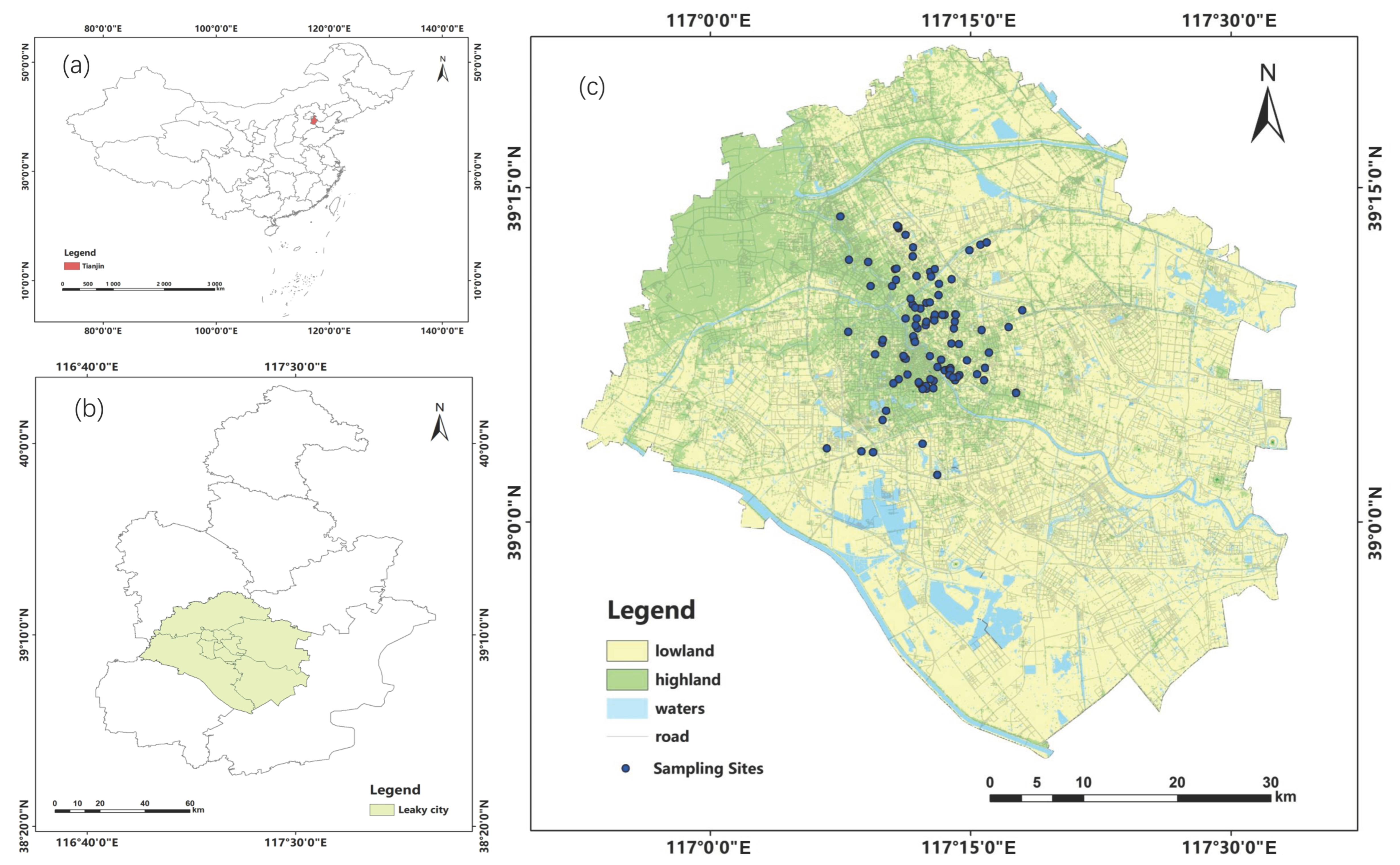
The study area is located in Tianjin city, which is an important central city in northern China. Geographically, Tianjin lies between 38°34′–40°15′N and 116°43′–118°04′E (see Figure 1a,b). The district consists of a coastal plain area in the east, a flat area in the middle, and a hilly and mountainous area in the northwest of the city (see Figure 1c). This area belongs to a temperate continental monsoon climate, the mean annual temperature is 14 °C, and the annual precipitation hovers around 360–970 mm. Winter is cold and dry, while summer is sweltering and muggy, with precipitation predominantly occurring in the latter part of summer and into autumn.
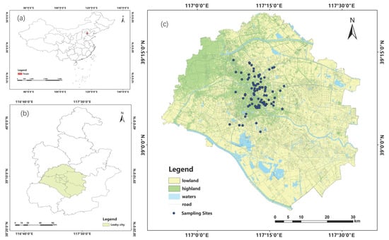
Figure 1.
Overview of the study area: (a) Location of Tianjin city in China; (b) Latitude–longitude coordinates of Tianjin city; (c) The distribution of 85 sampling sites in Tianjin city.
Tianjin is a water-scarce urban city. In 2022, Tianjin’s urban water pipeline network was 22,517.74 km long and delivered a total of 98,912.58 million cubic meters of water. However, the city’s water systems lost 13,552.40 million cubic meters, which is about 13.7 percent of the water used for public consumption (available online: https://www.mohurd.gov.cn/gongkai/fdzdgknr/sjfb/tjxx/jstjnj/index.html (accessed on 1 February 2025)). In addition, the total water savings of the study area in 2022 were merely 6.6 million cubic meters, which is significantly less than the total amount lost due to water pipeline leaks. Thus, it is a necessity to research and implement reliable, innovative leak detection technologies.
2.2. Data Collection and Preprocessing
Building an SSRDC prediction model is a systematic and complex process, and the preparation of training data is critical. This preparation involves both data collection and data processing. First, we acquire SAR data for the study area, using the backscattering coefficient of each pixel in the SAR image as input for the prediction model. Next, we select sampling sites and measure the SSRDC values at these sites using a GPR system, which serves as the target for the models.
2.2.1. SAOCOM-1A Data
The SAOCOM-1A L-band quad-polarization (HH, HV, VV, and VH) image was acquired in stripmap mode with ascending orbit direction and right-side observation. We select a SAOCOM-1A image acquired on 23 September 2021 during a dry period with almost no rainfall. The original image is the single-look complex (SLC) data with a spatial resolution of 10 m × 10 m. Data pre-processing work is carried out using the ENVI SARscape software (version 5.6). We process the data through four steps, including multi-looking, Lee filtering, geocoding, and radiometric calibration. After the pre-processing steps, the SAOCOM-1A images are converted to backscattering coefficient ; the values of vary approximately from −35 dB to 5 dB.
2.2.2. GPR System
The water pipeline leakage can cause an increase in the surrounding soil moisture content. Considering that the increase in subsurface soil moisture content will cause the increase in the soil dielectric constant. The dielectric constant of dry soil is approximately 3, and the dielectric constant of liquid water is 81 [28]. In addition, Ref. [28] indicates that the dielectric constant of soil is strongly dependent on soil moisture content and only weakly dependent on soil type, density, temperature, and the frequency range of 20 MHz to 1 GHz. Therefore, the location of pipeline water leakage can be inferred by measuring the soil dielectric constant. However, it is unrealistic to directly measure the subsurface soil moisture or dielectric constant by digging the ground. Here, we use a non-destructive measurement method based on GPR system. The review paper in [29] describes different methods for calculating the dielectric constant based on GPR measurement. In our paper, the reflected wave method is used to calculate the SSRDC. If the SSRDC at a sampling site exceeds a certain threshold, the site can be considered to have potential pipeline leakage.
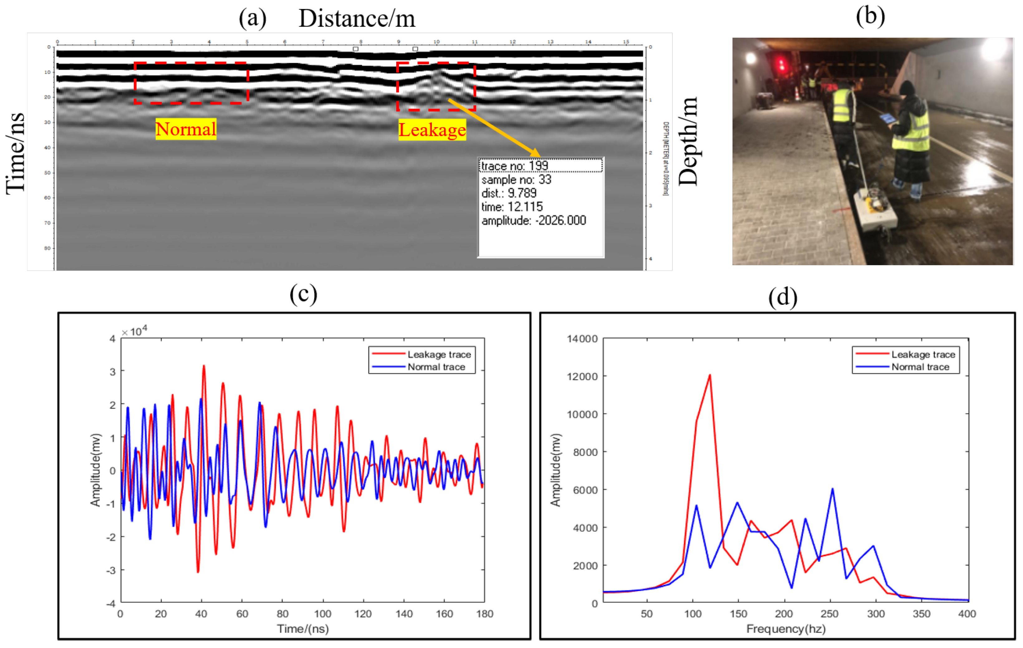
A GPR system includes a MALA ProEx unit and ground-coupled MALA 250 MHz frequency antennas. The antennas comprise transmitting and receiving antennas with a fixed spacing separation of 31 cm. The transmitting antenna emits an electromagnetic pulse into the ground, which is reflected back to the surface when it encounters subsurface discontinuities, such as soil, boundaries between different soil types, groundwater, or buried objects. The receiving antenna captures the reflected electromagnetic energy, allowing for the recording of raw data and the generation of high-resolution reflective images of subsurface features. After processing the raw data by the ReflexW software, the GPR B-scan image is presented in Figure 2a. The data processing approaches include subtracting DC-shift, moving start time, energy gain, background removal, bandpass Butterworth filter, and running average. First, we implement DC shift subtraction to correct system errors and remove DC offset, where the first time parameter is set to 66 ns and the second to 99 ns. Next, we adjust the initial sampling point to minimize interference. During this calibration, we record the time value at the first wave trough or peak and set the move time parameter to −14 ns. Then, energy gain is applied to enhance the signal amplitude, with a scaling factor set to 0.47. We utilize a bandpass Butterworth filter to eliminate signals outside the designated frequency range. In ReflexW, a lower cutoff frequency is set to 100 MHz and an upper cutoff frequency is set to 400 MHz. Finally, a running average is computed on each trace.
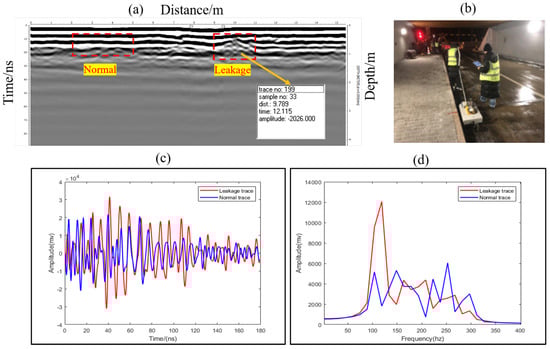
Figure 2.
GPR survey: (a) A GPR B-scan image after preprocessing; (b) Surveyor drives the GPR system; (c) The amplitude–time curves of the GPR traces; (d) The amplitude–frequency curves of the GPR traces.
Figure 2a shows a B-scan profile with leakage and non-leakage areas. In this profile, the reflected waves of leakage area have significant amplitude variations, phase shifts, or waveform distortions. In contrast, reflected waves in non-leakage areas remain relatively stable and consistent. During the measurement, the surveyor drives the equipment system along the measurement line, as shown in Figure 2b. When the antenna reaches each sampling site, its position is manually marked on the data. Meanwhile, the GPR traces are recorded in a .mrk file, which is utilized for calculating the SSRDC values. Analyzing the leak and non-leak traces, the time and frequency domain curves are shown in Figure 2c,d, where the higher moisture content can lead to greater reflected amplitudes. Higher moisture content generally increases the dielectric constant of the soil: when GPR waves encounter interfaces between materials with different dielectric constants, such as the wet and dry soil, this creates a stronger reflection of electromagnetic waves at these interfaces [30].
2.2.3. Measurement of SSRDC with GPR
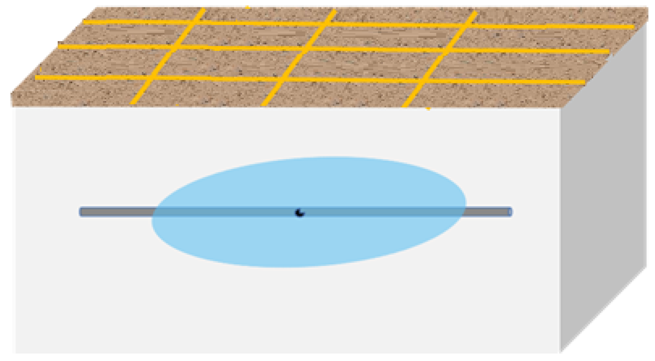
The field measurements of the SSRDC were performed simultaneously with the dates of acquisition of SAOCOM-1A satellite images. Coincident with the SAOCOM-1A satellite overpasses, each sampling site is 10 m × 10 m with no overlap between them, the coordinate data are recorded with a GPS, and the site is relatively flat. Within the sampling site, the SSRDC was measured using a GPR system. To reduce the measurement error, the SSRDC of each sampling site is computed by averaging the SSRDC values obtained from measurement points distributed within the site. The GPR followed 6 horizontal and vertical tracks with a spacing of 3 m between the acquisition tracks, as shown in Figure 3.
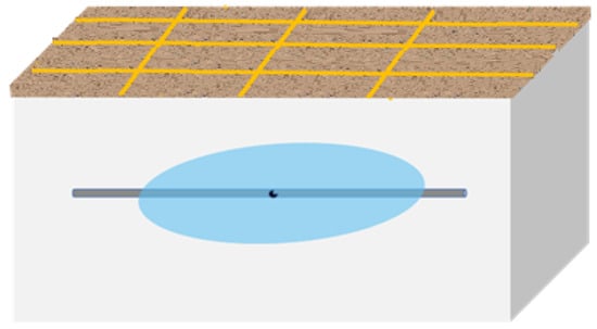
Figure 3.
The GPR follows 6 horizontal and vertical tracks.
The SSRDC values at sampling locations are calculated with the reflected wave method [31] based on the GPR data. The reflected wave methods are divided into two categories: single-offset and multi-offset measurements. The common midpoint (CMP) and wide-angle reflection and refraction (WARR) measurements are also called multi-offset measurements. We use the single-offset measurement to calculate the SSRDC; it is necessary to know the two-way travel time and the actual depth of the pipeline leakage target. The water pipeline leakage causes an increase in the surrounding soil moisture content: higher moisture content generally increases the dielectric constant of the soil [30]. When the electromagnetic waves pass through the leakage area, this creates a strong reflection of electromagnetic waves at reflection interfaces between materials with different dielectric constants, and the reflected waves have low energy, low frequency, and high amplitude characteristics. Thus, we infer the reflection interface based on the abnormal features of the reflected waves. Furthermore, the SSRDC value is calculated based on the actual depth of the leakage interface and the two-way travel time. For each sampling site, experienced leakage inspectors manually mark the leakage interfaces using Reflexw software in B-scan images that are obtained from 6 different tracks, as shown in Figure 4.
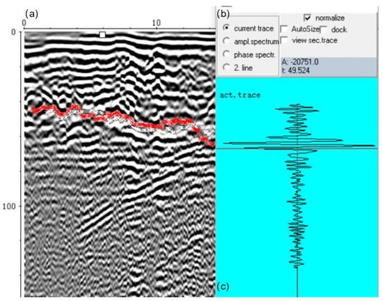
Figure 4.
(a) Leakage interface on the GPR B-scan image; (b) the amplitude and two-way travel time recorded by the Reflexw software; (c) GPR A-scan data obtained from a leakage area.
To verify and repair the pipeline leakage, we excavated the ground to expose the leakage point and measured the average depth d of the leakage interface. In each sampling site, 60 points are sparsely selected at equal intervals from the leakage interfaces, and we obtain A-scans of 60 points. For an A-scan, we extract the two-way travel time t of the reflected wave to leakage interface. In [31], the average velocity of the electromagnetic wave reaching the leakage interface, v, can be determined by
where x is the distance between the transmitted and received antennas of GPR. In a sampling site, the two-way travel times t of the reflected waves of 60 points are obtained from the corresponding A-scans, and the average velocities v of the reflected waves can be calculated by Equation (1). The results of t and v are shown in Table 1. The subsurface soil of the study area belongs to low-saline sandy soil with low-loss property; the SSRDC value of every point can be estimated by following the following equation [32]:
where c is 3 m/s. In Table 1, the SSRDC values of 60 points are calculated by Equation (2), and the SSRDC of a sampling site is computed by averaging the SSRDC values of 60 points.

Table 1.
Calculation results of subsurface soil relative dielectric constant (SSRDC) in a sampling site.
To ensure the rationality of the estimated SSRDC, we excavated the ground and exposed the leakage location to determine the leakage degree. In general, if the leakage degree is more severe, the measured SSRDC value is larger. For sampling sites that do not follow the above patterns, we remove them from the experimental data. Ultimately, 85 sampling sites (see Figure 1c) were collected in the study area, and the calculation results of SSRDC are shown in Table 2. The SSRDC value increases with the degree of leakage. The sampling site with ID-5 has a serious pipeline leak, and the SSRDC value of this point is relatively large, which is 26.51. The ID-2 sampling site has a minor leak, and the SSRDC value is 10.16.
Table 2.
Calculation results of SSRDC in 85 sampling sites.
2.3. Feature Extraction and Selection
Using SAR backscattering coefficients to directly predict soil dielectric constant may have limitations, as these coefficients are affected by various factors such as soil properties, surface roughness, vegetation cover, and moisture content [33]. In contrast, polarization combinations can provide more feature dimensions, which help machine learning models to learn the complex relationships between input features and the soil dielectric constant. In this subsection, we extract the feature variables from preprocessed SAOCOM-1A imagery. Then, the Boruta algorithm is applied to select the most informative characteristic variables from the feature space.
2.3.1. Feature Variable Extraction
Full-polarimetric SAR data capture comprehensive scattering information by utilizing all possible polarization states of the radar signal [34]. We extract VH, VV, HH, and HV backscattering coefficients from SAOCOM-1A imagery. The backscattering coefficients of radar images with different polarization modes emphasize different features of ground objects. For instance, water usually exhibits greater temporal variability in the VV polarization than in the HH polarization [35]. Moreover, L-band SAR cross-polarization (HV and VH) generally exhibit largely improved sensitivity compared with conventional co-polarization (VV and HH). Meanwhile, some research has indicated that relying solely on single-polarimetric data for model inputs may not yield optimal outcomes [36]. Therefore, it is essential to incorporate various polarization combinations as the feature variables in the prediction models. Based on the SAOCOM-1A imagery, 26 feature variables are extracted as candidate variables for the regression model (see Table 3), including 4 single-polarimetric variables and 22 polarization combination variables.
Table 3.
Feature variables extracted from SAR data.
2.3.2. Feature Variable Selection
A total of 26 candidate feature variables of the regression model were extracted with SAR data. However, when the number of variables greatly exceeds the optimal level, the accuracy of the regression model declines [37]. Feature variable selection is used to obtain optimal features from a larger set of features. Generally, principal component analysis (PCA) [38] and singular-value decomposition (SVD) [39] are considered to reduce the dimensionality of data. These techniques are unsupervised methods of feature selection, which do not take into account information between feature variables and outcome variables. The Boruta algorithm aims to identify all the important features that are relevant to the outcome variable. In this study, the Boruta algorithm is chosen due to its ability to capture nonlinear relationships and its robust discriminative power compared to classical statistical methods [40].
The Boruta algorithm is a wrapper that can iteratively remove irrelevant features. This algorithm classifies all variables into important, tentative, and unimportant [41]. The selection of important variables is based on their importance scores, which reflect their contribution to the regression model. The Boruta algorithm consists of three key steps. Firstly, it creates a copy of the original dataset and generates random shadow features for each attribute by randomly rearranging their values. This process helps to mitigate collinearity with the independent variables. Secondly, the algorithm calculates Z-scores by comparing the magnitudes of the true feature values with those of the shadow features at each iteration. Thirdly, the Boruta algorithm evaluates the importance of each feature by comparing the Z-scores, and classifies all attributes into important, unimportant, and tentative groups. The attributes that have higher Z-scores compared to shadow features are considered important. This algorithm was performed in the computer program R3.6.3 using the package “Boruta”.
2.4. Models
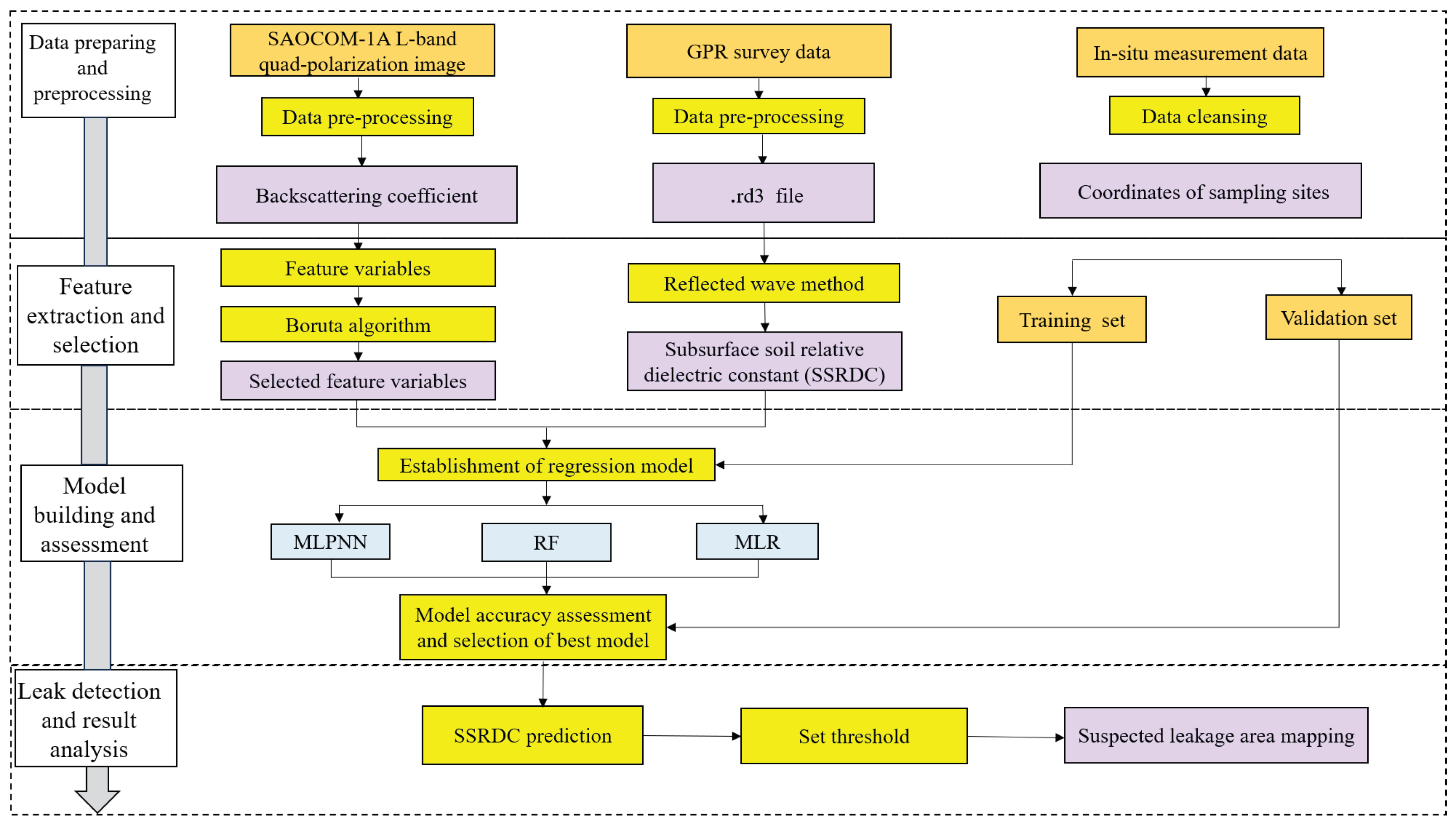
We develop three regression models to predict SSRDC values. The input variables for the regression models consist of the polarized combination features derived from the backscatter coefficients of each pixel in the SAR imagery, while the output variable is the SSRDC. We utilize the MLPNN, RF, and MLR to train three regression models based on the feature variables and the SSRDC measurement values of sampling sites. We evaluate the MLR, RF, and MLPNN models for their ability to predict the SSRDC values using the SAOCOM-1A imagery. A flowchart of the proposed method is shown in Figure 5.
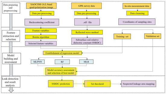
Figure 5.
Flowchart of the proposed method for detecting the pipeline leaks based on the SAOCOM-1A image and the GPR data.
2.4.1. Machine Learning Regression Model
In [42,43,44], the machine learning regression models have been used to predict soil moisture based on SAR data. In this paper, we present three methods to train the regression models based on the SAOCOM-1A image and the GPR data. The MLR, RF, and MLPNN methods are used to fit the complex relationships between the input and output variables, with the selected features serving as input variables and measured SSRDC as the output variable.
(1) Multiple Linear Regression
MLR is a widely utilized statistical method primarily aimed at establishing a linear model that relates a dependent variable to several independent variables. In comparison to simple linear regression, the inclusion of multiple independent variables enhances the accuracy of the regression, providing a more nuanced reflection of changes in the dependent variable. By thoughtfully increasing both the variety and number of independent variables, one can improve the model’s fit and strengthen its capacity to predict trends in the dependent variable. Thus, the introduced independent variables must be statistically reasonable and explanatory to prevent overfitting.
The general form of a MLR model is
where is the dependent variable, contains the independent feature variables, n is the number of variables, contains unknown parameters, and b is the error term. The best-fit line in regression analysis is found by minimizing the sum of squared variances between the actual data point and the corresponding points on that line. These differences are called residuals and represent the vertical distance from each observed data point to the straight line.
In an MLR model, the goal is to find a set of regression coefficients that minimizes the sum of squares of residuals between the predicted and observed values. The loss function used by the least squares method is the residual sum of squares (RSS), which accurately represents the sum of squares of the difference between the measured values and predicted values of m sampling sites, as follows:
By minimizing the RSS, we can determine the optimal regression coefficients and error term, which allows the model to better fit the data and improve the accuracy of the prediction.
(2) Random Forest
RF algorithm is a predictive model composed of multiple decision trees, each implementing a distinct method for making predictions. Specifically, each tree classifies the data using its own criteria and then classifies the data by assigning as many pixels as possible to the corresponding category [45]. The process is as follows. Firstly, n samples are extracted from the original sample set, multiple subsample sets are constructed, and then n decision trees are constructed based on these subsample sets [46,47]. In the growth process of the decision tree, m features (the total number of features is M, ) are randomly selected from each node of each tree, and the features with the highest classification power are chosen based on the criterion of minimizing the Gini coefficient. Finally, the RF classifier is formed by the generated decision tree, and the regression results are obtained by means of average. In this process, two parameters need to be set: the number of decision trees N and the number of features per node of each tree m. RF is widely utilized in remote sensing for regression tasks, benefiting from its ability to handle a large number of input features while maintaining low computational costs [48,49].
(3) Multi-Layer Perceptron Neural Network
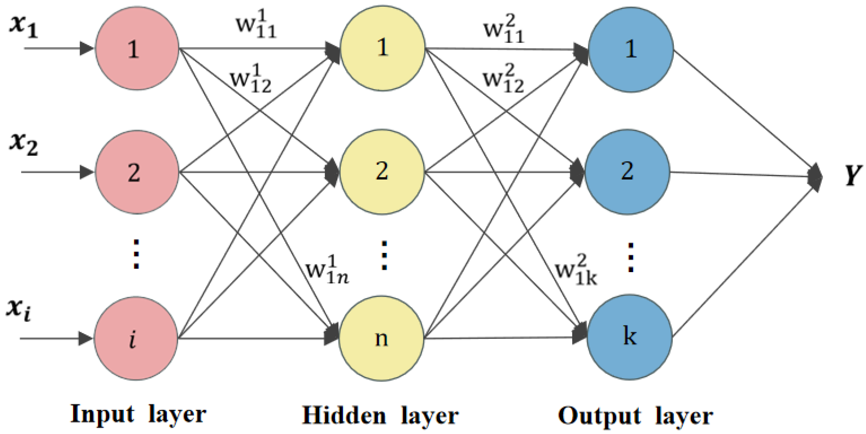
MLPNN consists of an input layer, an output layer, and at least one hidden layer, as shown in Figure 6. The hidden layer contains multiple neurons that receive the output and weights of the previous layer and perform nonlinear transformations via activation functions to learn complex relationships in the data [50]. The output layer receives the output from the last hidden layer and converts it into the final predicted result. The number of neurons in the output layer usually matches the number of classes or output dimensions that the model needs to distinguish [51,52,53,54]. Neural networks can effectively model the nonlinear relationship between input and output layers.
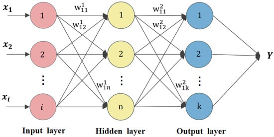
Figure 6.
Multi-layer perceptron neural network (MLPNN) structure.
2.4.2. Model Evaluation
We use the root mean square error (RMSE), the coefficient of determination (), and mean absolute error (MAE) to evaluate the performance of three machine learning regression models. The three statistical indicators are widely used in regression analysis models to assess the difference between the observed and predicted values [55,56]. RMSE and MAE can intuitively measure the prediction error of the model, reflecting the accuracy of the model. represents the proportion of target variance that can be explained by the model: a higher value indicates better model performance. They can be calculated by
where represents the measured SSRDC of the i-th sampling site, represents the predicted SSRDC of i-th site, and represents the average value of field-measured SSRDC.
3. Results
3.1. Feature Variable Selection Result
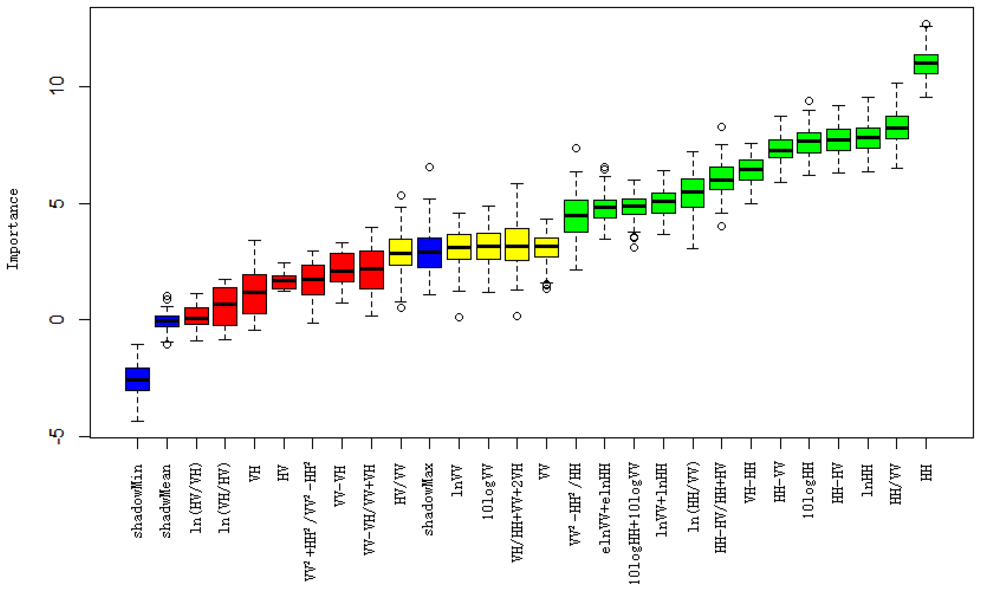
Utilizing SAOCOM-1A imagery, we first extracted 26 feature variables as candidate variables for our regression models. These variables included 4 single-polarimetric variables and 22 polarization combination variables (Table 3). Then, we used the Boruta algorithm package in R-3.6.4 for feature selection; the maximum number of iterations was assigned a value of 300, and other parameters were set to their default values. The results of the importance of all feature variables are shown in Figure 7, from which we selected 13 feature variables with high importance. Further, we calculated the Pearson correlation coefficients between 13 selected variables. If the correlation coefficient between two variables is greater than 0.8, the one with lower importance is removed. Ultimately, we retain 10 features with lower correlations and take them as inputs to the regression model—see Table 4.
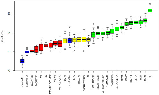
Figure 7.
Importance results of all feature variables.
Table 4.
Feature variable selection results based on Boruta.
The selected feature variables are mostly composed of HH and VV polarization combinations, as the penetration ability of the same polarization is greater than that of cross-polarization. In [57], the experimental result shows that the HH/VV co-polarized backscatter coefficient is used to represent soil dielectric constant and surface roughness. For variable HH − HV, the difference between HH polarization and HV polarization can obtain soil information under the impermeable layer; the feature variable can be used for leak detection. The feature VH/(HH + VV + 2VH) can eliminate the influence of urban vegetation on soil moisture measurements. Other feature derived from soil moisture retrieval studies are related to soil dielectric constant and can serve as feature variables in regression models.
3.2. Model Training and Validation
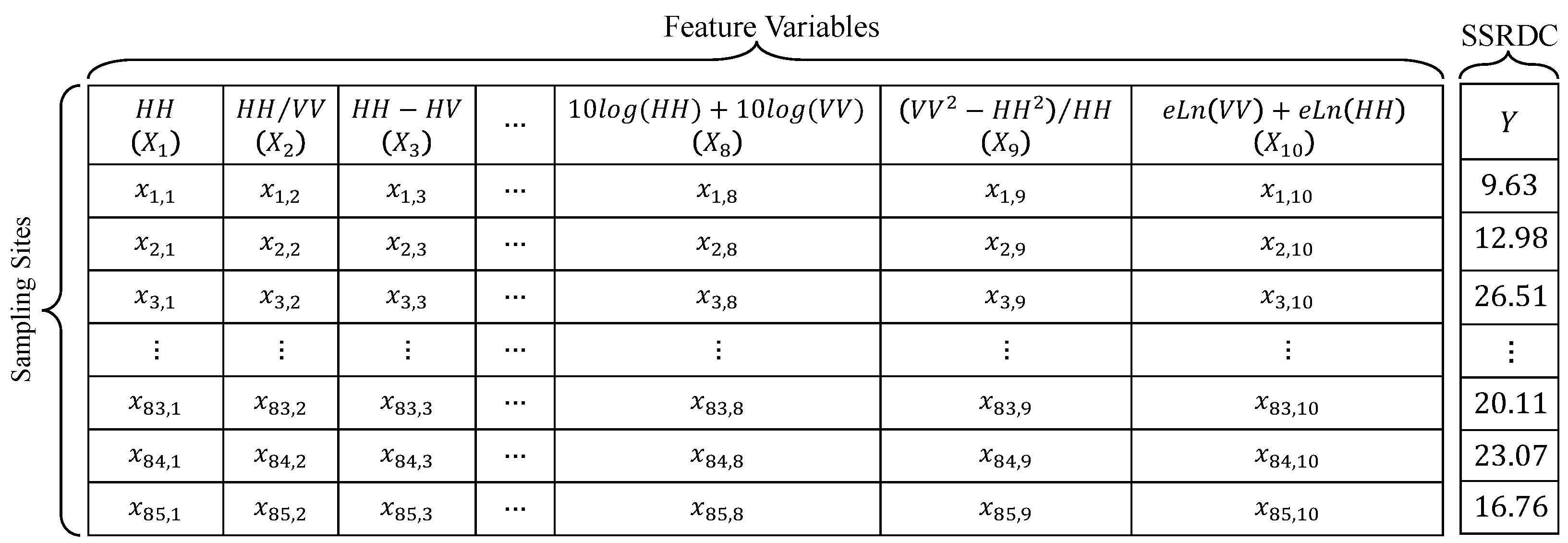
We collected 85 high-quality sampling sites with different degrees of leakage. Using sampling sites with different degrees of leakage helps to improve the accuracy of the regression model. The data collected for each sample site include 10 feature values and the estimated SSRDC value. The data for all sample sites are prepared and organized as shown in Figure 8. All sites can be arranged row by row, while their 10 feature values and the estimated SSRDC value are arranged column by column. Columns 1 to 10 correspond to the 10 features, and the last column corresponds to the estimated SSRDC.

Figure 8.
Training and validation datasets for all sampling sites.
We divided the complete set of 85 samples into a training set and a validation set, with 42 samples in the training set and 43 samples in the validation set. We applied three statistical metrics (, RMSE, MAE) to evaluate the regression models by using the validation dataset.
We run the MLR algorithm using the LinearRegression function from sklearn.linear model library, and run the RF algorithm with trees using the RandomForestRegressor.svm function from sklearn.ensemble library with the default parameter settings. By training the regression models with the collected dataset, we obtained the regression coefficients and error term of the MLR model, as well as the parameters of the RF model.
The number of neurons in the output layer of the network is consistent with the expected number of classifications, and the number of neurons in the input layer is aligned with the number of attributes. The number of hidden layers and neurons is uncertain. Although adding hidden layers can improve classification accuracy and meet specific recognition requirements, networks with multiple hidden layers are often more prone to training problems compared to networks with a single hidden layer [54]. As a result, our network has one hidden layer. Different numbers of hidden layer neurons were attempted, ranging from 1 to 10. When the number of neurons in the hidden layer increases from 1 to 7, increases from 0.583 to 0.705. However, as the number of hidden neurons continues to increase, it is found that the predictive performance actually decreases. Thus, the SSRDC is estimated by using a neural network with ten input neurons, seven hidden neurons, and one output neuron.
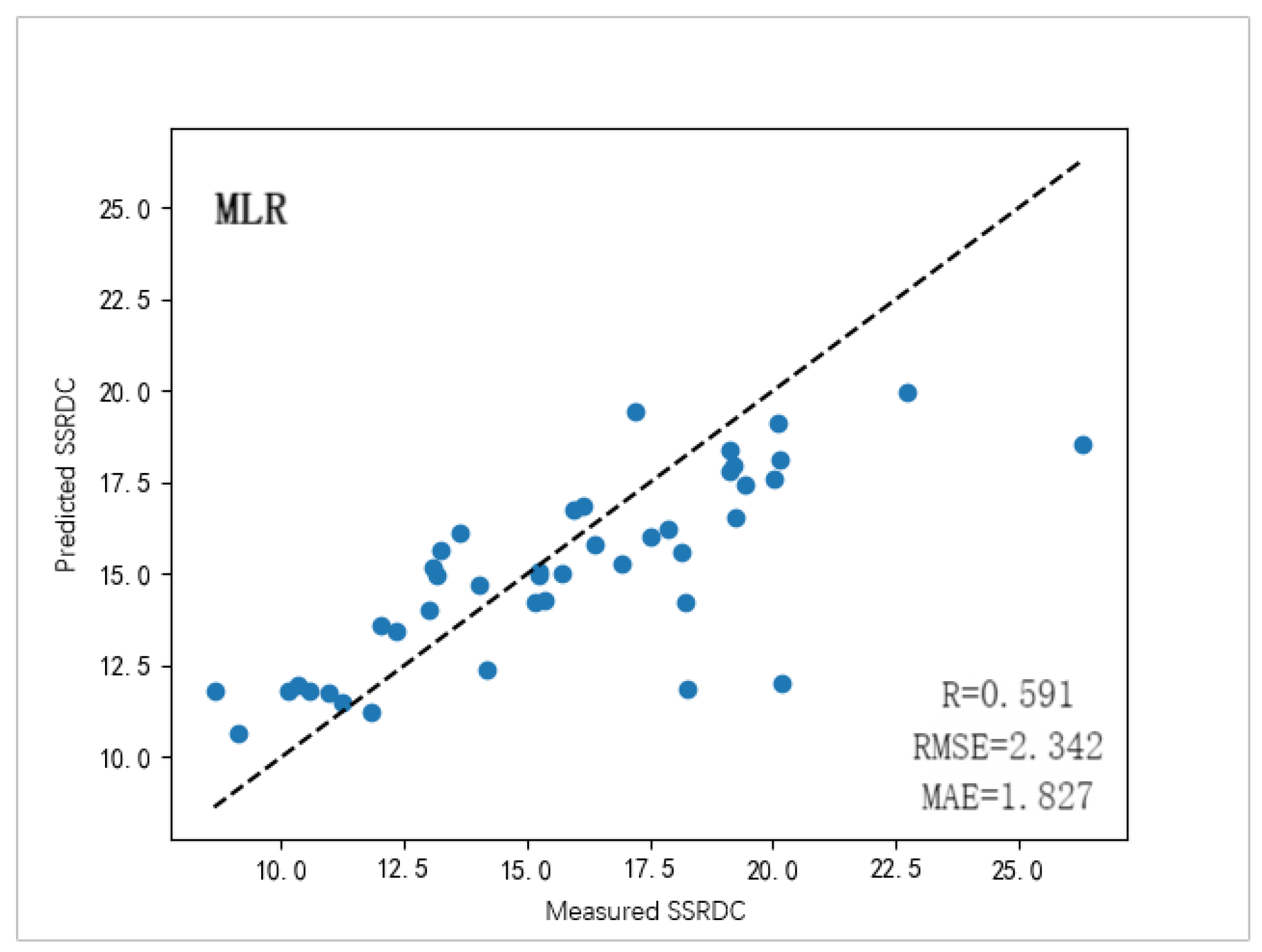
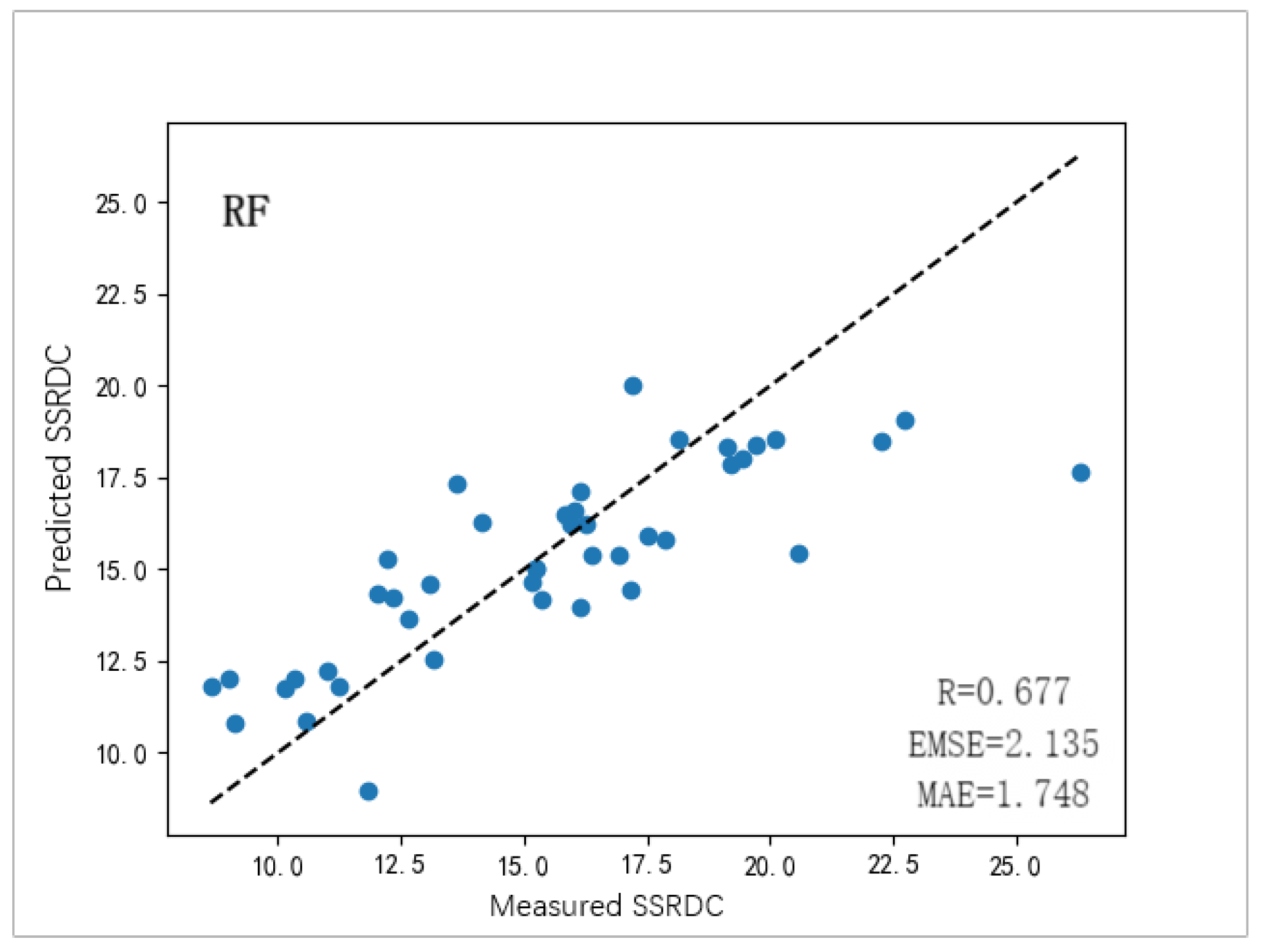
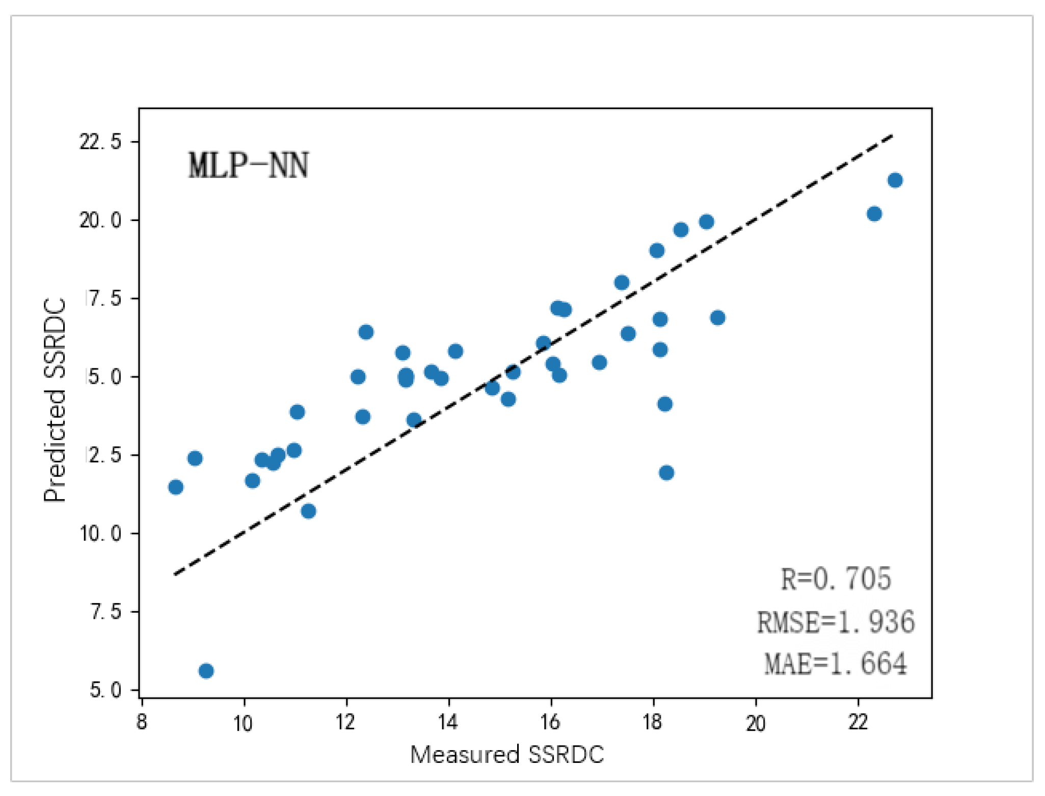
Table 5 shows the performance of leak detection models in the validation dataset. The MLR model exhibits a low coefficient of determination ( = 0.591), high root mean square error (RMSE = 2.342), high mean absolute error (MAE = 1.827), poor predictive performance, and low fit. On the contrary, the MLPNN model exhibits a high coefficient of determination ( = 0.705), small root mean square error (RMSE = 1.936), small mean absolute error (MAE = 1.664), excellent predictive performance, and good fit in Figure 9, Figure 10 and Figure 11. Overall, the MLPNN model has high fitting accuracy and small errors for sample points. By comprehensively comparing the evaluation indicators of the three models, the predictive performance of dielectric constant estimation is as follows: MLPNN > RF > MLR. Therefore, the MLPNN model can more accurately achieve dielectric constant inversion. For n sample sites, the computational complexities of the MLR and RF models are and , respectively. The MLPNN computation each iteration occupies complexity. The MLPNN model has the highest accuracy in estimating SSRDC on the study area, but it requires more processing time than the MLR and RF models.
Table 5.
Performance of leak detection models on the validation dataset.
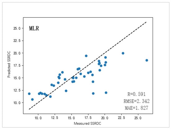
Figure 9.
Result of MLR.

Figure 10.
Result of RF.
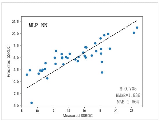
Figure 11.
Result of MLPNN.
3.3. Leak Detection Result
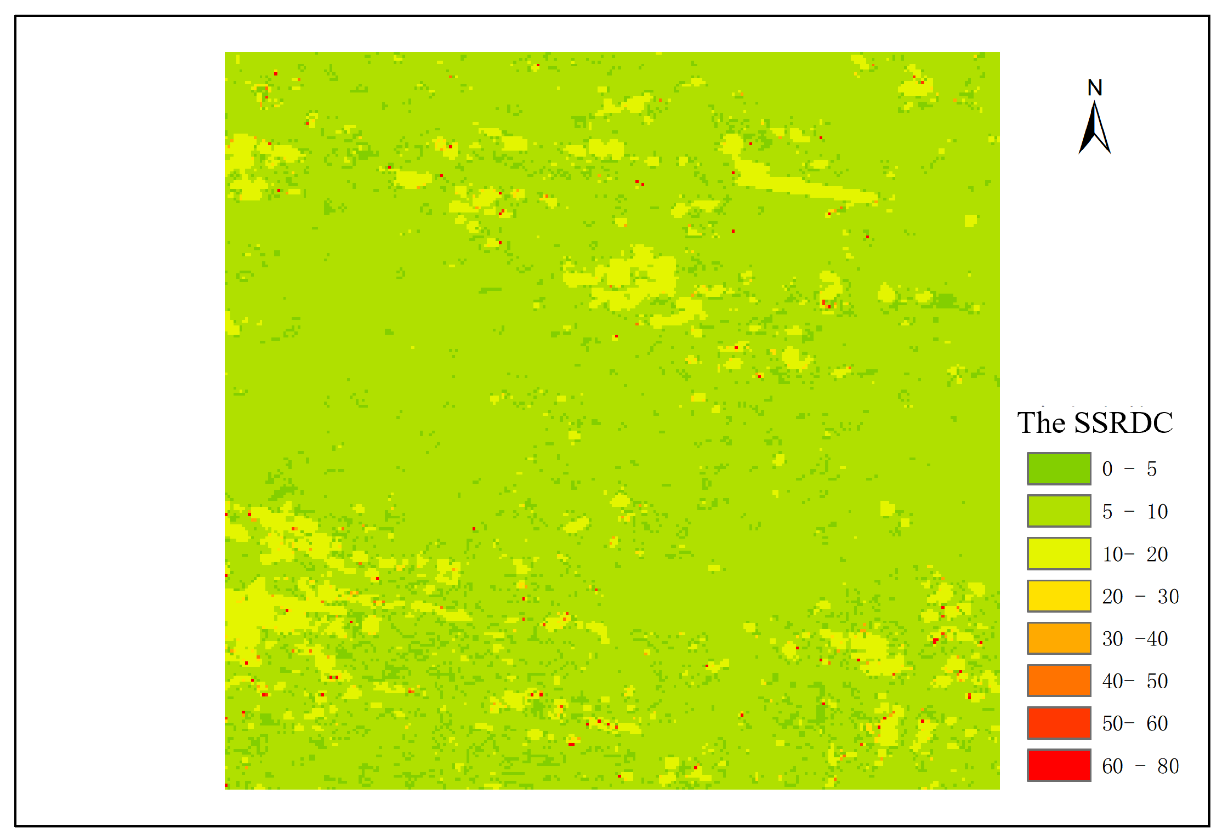
Based on the fully polarized SAOCOM-1A data and GPR measured data, we have developed three SSRDC predictive models. A comparison of the evaluation indices across different models indicated that the MLPNN model yielded the best performance, and it was subsequently employed for dielectric constant inversion in the study area. In contrast to the study area used for training and validating the regression model, we selected a new area for leak detection. We first acquired SAR imagery from a new area, then extracted feature values from the SAR images and input them into the developed prediction model to obtain the SSRDC values for all locations. The results indicated that the predicted SSRDC values generally fall within the range of 0 to 30 (Figure 12), which is consistent with the SSRDC values measured by GPR.
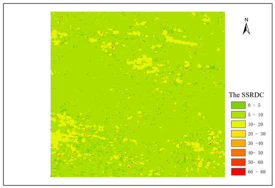
Figure 12.
SSRDC prediction results.
We consider locations where the predicted SSDRC values exceed a certain threshold as potential leak locations. In Figure 12, all points that fall on the pipes are sorted in descending order according to the predicted SSDRC values. The top 10% of points are identified as possible leakage points, and the threshold is defined as the minimum predicted SSDRC value among these points. Here, 10% are empirical data, which is the probability of urban pipeline leakage from a water supply company’s survey data. In this area, the threshold is approximately 10. The threshold may be influenced by soil moisture conditions; this threshold selection method combined the empirical data and the predicted SSRDC data, which could be applied to various areas.
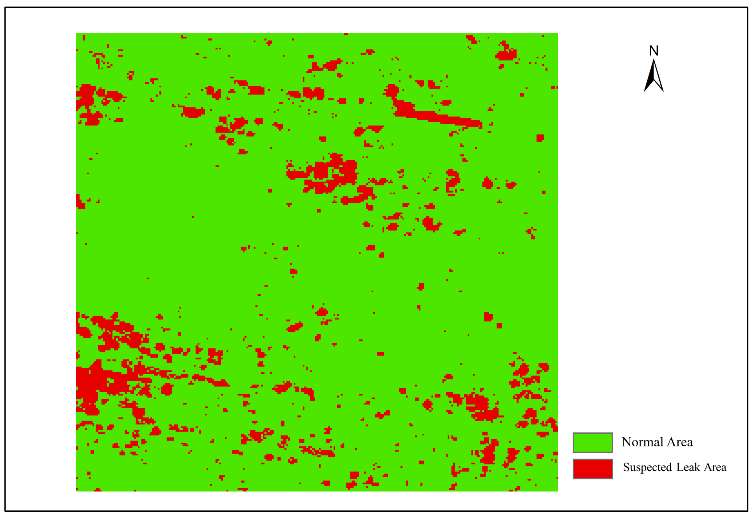
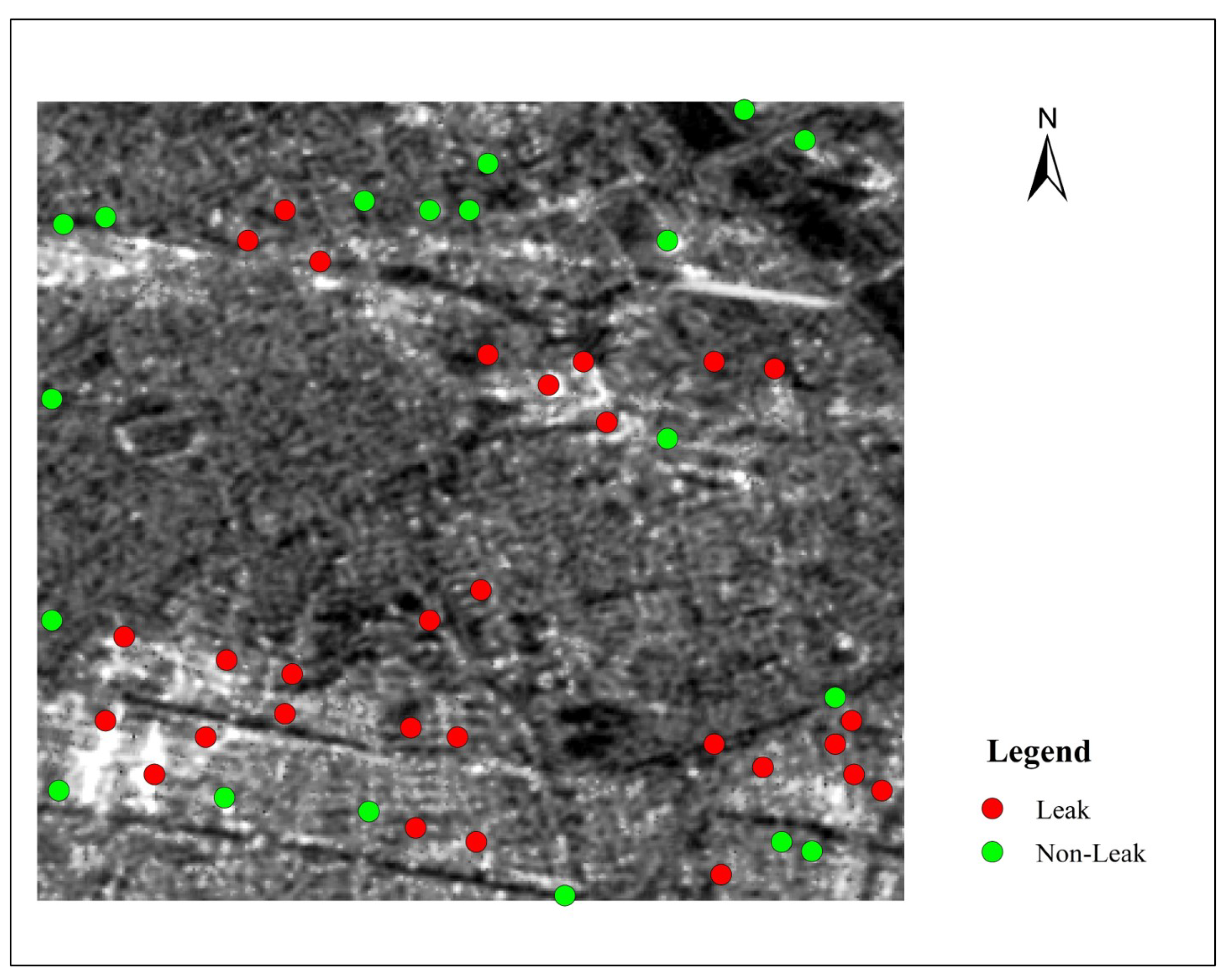
In Figure 13, most of the suspected leakage areas extracted showed a planar aggregation distribution, indicating that the detection results are highly reliable. The extracted suspected leakage area and pipe network data are superimposed under the same spatial reference, and the area with an abnormal dielectric constant caused by other reasons is eliminated to obtain the suspected leakage locations. The field verification is produced at 48 suspected leakage locations. In Figure 14, leakage is found at the red points, while no leakage is detected at the green points. As a result, the accuracy of the model’s leakage detection is 60.42%. The empirical results indicate an encouraging potential of the proposed method to locate the pipeline leaks.
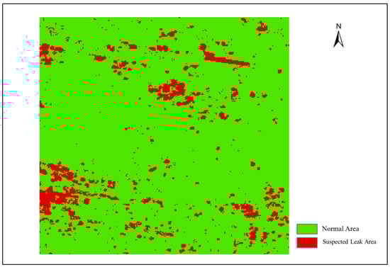
Figure 13.
Suspected leakage area.

Figure 14.
Leak detection result.
We also train a 0–1 classification model using SAR data and leak/non-leak data. Due to the limited training data, the accuracy of the classification model is relatively low. In addition, we use only GPR data and the wave reflection method to detect pipeline leaks, achieving approximately 75% accuracy. However, the GPR method requires manual operation, making it difficult to detect rapidly in large areas. This paper combines SAR and GPR data to develop a regression model. The regression model estimates SSRDC values based on polarization combination features of SAR. Compared to the leak/non-leak classification model, our approach uses more detailed sampling data to train regression models and it obtains better results. Moreover, the SAR-based leakage detection method is more suitable for large-scale, rapid detection in a short period.
4. Discussion
(1) Feature Variable Extraction
Effective feature extraction plays a crucial role in accurately predicting the SSRDC values, which are pivotal for identifying water pipeline leaks. The feature selection process using the Boruta algorithm is particularly advantageous due to its ability to handle interactions among features and its capacity for identifying important variables without overfitting. This is significant for our regression models because irrelevant or redundant features could obscure the relationship between the independent variables and the SSRDC values. Future work could explore the impact of environmental factors on SSRDC, such as variations in soil moisture or temperature.
(2) SSRDC Estimation
The SSRDC values at sampling locations are calculated with the reflected wave method, which has some limitations. Firstly, the method requires the actual leakage depth to be known, which may have errors in the actual measurement. Because of the complex underground environment, there are errors in determining the leakage interface. Secondly, leakage phenomena are often accompanied by problems such as land subsidence and urban cavities. The interference signals caused by these problems are easy to be confused with the leakage signals, resulting in a deviation in the selection of leakage interface, thus affecting the accuracy and reliability of the reflected wave method. Furthermore, we utilize the richer information from reflected waves to estimate the dielectric constant in order to improve the estimation accuracy.
(3) Model Accuracy
This article uses fully polarized SAOCOM-1A satellite images, with the constructed polarization combination index and dielectric constant as feature variables and machine learning algorithms as modeling methods. Through a comparison of model evaluation indicators, MLPNN has the best detection model evaluation indicators: = 0.705, RMSE = 1.936, MAE = 1.664. For the problems of small sample size and insufficient data diversity in the experiment, we will continue to cooperate with the water company to collect more first-hand leaked data to enrich the sample size. At the same time, we will use GAN and Diffusion Model methods in deep learning to expand the sample data and improve the robustness and universality of downstream training models. After increasing or expanding the sample data, deep learning methods can be introduced for regression fitting to improve the accuracy of model detection.
5. Conclusions
We interpreted the problem of detecting the pipeline leakage as a regression problem and presented a method by combining the SAOCOM-1A image and the GPR data to develop the MLPNN, RF, and MLR regression models. The method makes use of the Boruta algorithm to select feature variables based on the SAOCOM-1A images after pre-processing, and calculated the SSRDC values of sampling locations with reflected wave algorithm based on the GPR data. We evaluated three regression models for their ability to predict the SSRDC values using the selected features. The experimental results show that, compared with the RF and MLR models, the MLPNN model can better estimate the SSRDC values. The MLPNN possesses strong nonlinear modeling capabilities, allowing it to fit complex features through multiple hidden layers. This enables it to effectively capture the intricate relationships between input features, resulting in superior performance when processing the complex nonlinear relationship between SSDRC and the radar image backscattering coefficient. After obtaining the optimal SSRDC prediction model, we acquired the SAR imagery of a new area. We then extracted feature values from the SAR images and input them into the developed prediction model to obtain the SSRDC values for all locations. The locations with higher SSRDC values were identified as potential leak points; a total of 48 suspected leak areas were detected, of which 29 had leak points, with a detection accuracy of 60%. Experimental results verify the applicability and effectiveness of regression models. Overall, our method can achieve the rapid, large-scale, and non-destructive detection of leaks in water supply networks and give a satisfying result.
Author Contributions
Conceptualization, F.D. and Y.Z.; methodology, F.D. and Y.Z.; software, Y.Z.; validation, F.D., Y.Z. and H.G.; formal analysis, Y.Z.; investigation, Y.Z.; resources, H.G.; data curation, F.D.; writing—original draft preparation, Y.Z.; writing—review and editing, F.D. and H.G.; visualization, Y.Z.; supervision, H.G. and F.D.; project administration, H.G. and F.D.; funding acquisition, H.G. All authors have read and agreed to the published version of the manuscript.
Funding
This research was funded by the Research Project on Leakage Detection Method of Urban Water Supply Network based on Long-wave Radar Satellite Image (No. 24220010038) and Construction Funding for the Engineering Research Center of Ministry of Education on Spatial Information Technology (No. 24550110002).
Data Availability Statement
The data that support the findings of this study are available from the corresponding author, upon reasonable request.
Acknowledgments
The authors are grateful to the Tianjin Water Group Co., Ltd., for providing the in situ data used in this study. We would also like to thank the editors and the anonymous reviewers for their valuable comments.
Conflicts of Interest
The authors declare no conflicts of interest.
References
- Meng, L.; Li, Y.; Wang, W.; Fu, J. Experimental study on leak detection and location for gas pipeline based on acoustic method. J. Loss Prev. Process Ind. 2012, 25, 90–102. [Google Scholar] [CrossRef]
- Lee, S.; Kim, B. Machine learning model for leak detection using water pipeline vibration sensor. Sensors 2023, 23, 8935. [Google Scholar] [CrossRef]
- Singh, S.; Agrawal, S.; Sahu, T.; Das, D. iPipe: Water pipeline monitoring and leakage detection. In Proceedings of the 2021 IEEE International Symposium on Smart Electronic Systems (ISES), Jaipur, India, 18–22 December 2021; pp. 367–372. [Google Scholar]
- Lim, K.; Wong, L.; Chiu, W.K.; Kodikara, J. Distributed fiber optic sensors for monitoring pressure and stiffness changes in out-of-round pipes. Struct. Control Health Monit. 2016, 23, 303–314. [Google Scholar] [CrossRef]
- Chen, Q.; Shen, G.; Jiang, J.; Diao, X.; Wang, Z.; Ni, L.; Dou, Z. Effect of rubber washers on leak location for assembled pressurized liquid pipeline based on negative pressure wave method. Process Saf. Environ. Prot. 2018, 119, 181–190. [Google Scholar] [CrossRef]
- Kam, S.I. Mechanistic modeling of pipeline leak detection at fixed inlet rate. J. Pet. Sci. Eng. 2010, 70, 145–156. [Google Scholar] [CrossRef]
- Li, X.; Chen, G.; Zhang, R.; Zhu, H.; Fu, J. Simulation and assessment of underwater gas release and dispersion from subsea gas pipelines leak. Process Saf. Environ. Prot. 2018, 119, 46–57. [Google Scholar]
- Gao, Y.; Liu, Y.; Ma, Y.; Cheng, X.; Yang, J. Application of the differentiation process into the correlation-based leak detection in urban pipeline networks. Mech. Syst. Signal Process. 2018, 112, 251–264. [Google Scholar] [CrossRef]
- Yin, S.; Weng, Y.; Song, Z.; Cheng, B.; Gu, H.; Wang, H.; Yao, J. Mass transfer characteristics of pipeline leak-before-break in a nuclear power station. Appl. Therm. Eng. 2018, 142, 194–202. [Google Scholar] [CrossRef]
- Cramer, R.; Shaw, D.; Tulalian, R.; Angelo, P.; van Stuijvenberg, M. Detecting and correcting pipeline leaks before they become a big problem. Mar. Technol. Soc. J. 2015, 49, 31–46. [Google Scholar] [CrossRef]
- Demirci, S.; Yigit, E.; Eskidemir, I.H.; Ozdemir, C. Ground penetrating radar imaging of water leaks from buried pipes based on back-projection method. NDT E Int. 2012, 47, 35–42. [Google Scholar] [CrossRef]
- Lai, W.W.; Chang, R.K.; Sham, J.F. A blind test of nondestructive underground void detection by ground penetrating radar (GPR). J. Appl. Geophys. 2018, 149, 10–17. [Google Scholar] [CrossRef]
- Ocaña-Levario, S.J.; Ayala-Cabrera, D.; Izquierdo, J.; Pérez-García, R. 3D model evolution of a leak based on GPR image interpretation. Water Sci. Technol. Water Supply 2015, 15, 1312–1319. [Google Scholar] [CrossRef]
- Zhao, W.; Forte, E.; Pipan, M.; Tian, G. Ground penetrating radar (GPR) attribute analysis for archaeological prospection. J. Appl. Geophys. 2013, 97, 107–117. [Google Scholar] [CrossRef]
- Atef, A.; Zayed, T.; Hawari, A.; Khader, M.; Moselhi, O. Multi-tier method using infrared photography and GPR to detect and locate water leaks. Autom. Constr. 2016, 61, 162–170. [Google Scholar] [CrossRef]
- Cataldo, A.; De Benedetto, E.; Cannazza, G.; Leucci, G.; De Giorgi, L.; Demitri, C. Enhancement of leak detection in pipelines through time-domain reflectometry/ground penetrating radar measurements. IET Sci. Meas. Technol. 2017, 11, 696–702. [Google Scholar] [CrossRef]
- Wunderlich, T.; Majchczack, B.S.; Wilken, D.; Segschneider, M.; Rabbel, W. What is beyond hyperbola detection and characterization in ground-penetrating radar data?—implications from the archaeological site of Goting, Germany. Remote Sens. 2024, 16, 4080. [Google Scholar] [CrossRef]
- Abdulraheem, M.I.; Chen, H.; Li, L.; Moshood, A.Y.; Zhang, W.; Xiong, Y.; Zhang, Y.; Taiwo, L.B.; Farooque, A.A.; Hu, J. Recent advances in dielectric properties-based soil water content measurements. Remote Sens. 2024, 16, 1328. [Google Scholar] [CrossRef]
- Guan, Y.; Grote, K. Assessing the potential of UAV-based multispectral and thermal data to estimate soil water content using geophysical methods. Remote Sens. 2023, 16, 61. [Google Scholar] [CrossRef]
- Lu, Q.; Liu, K.; Zeng, Z.; Liu, S.; Li, R.; Xia, L.; Guo, S.; Li, Z. Estimation of the soil water content using the early time signal of ground-penetrating radar in heterogeneous soil. Remote Sens. 2023, 15, 3026. [Google Scholar] [CrossRef]
- Zhang, J.; Zhang, C.; Lu, Y.; Zheng, T.; Dong, Z.; Tian, Y.; Jia, Y. In-situ recognition of moisture damage in bridge deck asphalt pavement with time-frequency features of GPR signal. Constr. Build. Mater. 2020, 244, 118295. [Google Scholar] [CrossRef]
- Shi, J.; Wang, J.; Hsu, A.Y.; O’Neill, P.E.; Engman, E.T. Estimation of bare surface soil moisture and surface roughness parameter using L-band SAR image data. IEEE Trans. Geosci. Remote Sens. 1997, 35, 1254–1266. [Google Scholar]
- Gururaj, P.; Umesh, P.; Shetty, A. Assessment of surface soil moisture from ALOS PALSAR-2 in small-scale maize fields using polarimetric decomposition technique. Acta Geophys. 2021, 69, 579–588. [Google Scholar] [CrossRef]
- Lasne, Y.; Paillou, P.; August-Bernex, T.; Ruffié, G.; Grandjean, G. A phase signature for detecting wet subsurface structures using polarimetric L-band SAR. IEEE Trans. Geosci. Remote Sens. 2004, 42, 1683–1694. [Google Scholar] [CrossRef]
- Mazzarotto, G.; Tessari, G.; Pizzaia, P.; Salandin, P. Identifying pipeline leak positions potentially connected to soil deformations through SAR data analysis. J. Infrastruct. Syst. 2023, 29, 04023017. [Google Scholar] [CrossRef]
- Pongrac, B.; Gleich, D. Polarimetric SAR based water leakage detection using 3D regression neural network. In Proceedings of the IGARSS 2022—2022 IEEE International Geoscience and Remote Sensing Symposium, Kuala Lumpur, Malaysia, 17–22 July 2022; pp. 3700–3703. [Google Scholar]
- Le, X.; Yu, H.; Wang, Y. An interpretable neural network algorithm for leaking detection in the urban water and sewer pipeline network, Tianjin, China. In Proceedings of the IGARSS 2023—2023 IEEE International Geoscience and Remote Sensing Symposium, Pasadena, CA, USA, 16–21 July 2023; pp. 2053–2056. [Google Scholar]
- Topp, G.C.; Davis, J.L.; Annan, A.P. Electromagnetic determination of soil water content: Measurements in coaxial transmission lines. Water Resour. Res. 1980, 16, 574–582. [Google Scholar] [CrossRef]
- Liu, X.; Chen, J.; Cui, X.; Liu, Q.; Cao, X.; Chen, X. Measurement of soil water content using ground-penetrating radar: A review of current methods. Int. J. Digit. Earth 2019, 12, 95–118. [Google Scholar] [CrossRef]
- Nakashima, Y.; Zhou, H.; Sato, M. Estimation of groundwater level by GPR in an area with multiple ambiguous reflections. J. Appl. Geophys. 2001, 47, 241–249. [Google Scholar] [CrossRef]
- Huisman, J.A.; Hubbard, S.S.; Redman, J.D.; Annan, A.P. Measuring soil water content with ground penetrating radar: A review. Vadose Zone J. 2003, 2, 476–491. [Google Scholar] [CrossRef]
- Davis, J.L.; Annan, A.P. Ground-penetrating radar for high-resolution mapping of soil and rock stratigraphy 1. Geophys. Prospect. 1989, 37, 531–551. [Google Scholar] [CrossRef]
- Xing, M.; Chen, L.; Wang, J.; Shang, J.; Huang, X. Soil moisture retrieval using SAR backscattering ratio method during the crop growing season. Remote Sens. 2022, 14, 3210. [Google Scholar] [CrossRef]
- Haldar, D.; Das, A.; Mohan, S.; Pal, O.; Hooda, R.S.; Chakraborty, M. Assessment of L-band SAR data at different polarization combinations for crop and other landuse classification. Prog. Electromagn. Res. B 2012, 36, 303–321. [Google Scholar] [CrossRef]
- Park, N.W.; Chi, K.H. Integration of multitemporal/polarization C-band SAR data sets for land-cover classification. Int. J. Remote Sens. 2008, 29, 4667–4688. [Google Scholar] [CrossRef]
- Lee, J.S.; Grunes, M.R.; Pottier, E. Quantitative comparison of classification capability: Fully polarimetric versus dual and single-polarization SAR. IEEE Trans. Geosci. Remote Sens. 2001, 39, 2343–2351. [Google Scholar]
- Kohavi, R.; John, G.H. Wrappers for feature subset selection. Artif. Intell. 1997, 97, 273–324. [Google Scholar] [CrossRef]
- Chamundeeswari, V.V.; Singh, D.; Singh, K. An analysis of texture measures in PCA-based unsupervised classification of SAR images. IEEE Geosci. Remote Sens. Lett. 2009, 6, 214–218. [Google Scholar] [CrossRef]
- Wall, M.E.; Rechtsteiner, A.; Rocha, L.M. Singular value decomposition and principal component analysis. In A Practical Approach to Microarray Data Analysis; Springer: Berlin/Heidelberg, Germany, 2003; pp. 91–109. [Google Scholar]
- Saleem, J.; Zakar, R.; Butt, M.S.; Aadil, R.M.; Ali, Z.; Bukhari, G.M.J.; Ishaq, M.; Fischer, F. Application of the Boruta algorithm to assess the multidimensional determinants of malnutrition among children under five years living in southern Punjab, Pakistan. BMC Public Health 2024, 24, 167. [Google Scholar] [CrossRef]
- Kursa, M.B.; Rudnicki, W.R. Feature selection with the Boruta package. J. Stat. Softw. 2010, 36, 1–13. [Google Scholar] [CrossRef]
- Wang, J.; Wang, W.; Hu, Y.; Tian, S.; Liu, D. Soil moisture and salinity inversion based on new remote sensing index and neural network at a salina-alkaline wetland. Water 2021, 13, 2762. [Google Scholar] [CrossRef]
- Wang, J.; Wu, F.; Shang, J.; Zhou, Q.; Ahmad, I.; Zhou, G. Saline soil moisture mapping using Sentinel-1A synthetic aperture radar data and machine learning algorithms in humid region of China’s east coast. Catena 2022, 213, 106189. [Google Scholar] [CrossRef]
- Yadav, V.P.; Prasad, R.; Bala, R.; Vishwakarma, A.K. An improved inversion algorithm for spatio-temporal retrieval of soil moisture through modified water cloud model using C-band Sentinel-1A SAR data. Comput. Electron. Agric. 2020, 173, 105447. [Google Scholar] [CrossRef]
- Zhang, N.; Chen, M.; Yang, F.; Yang, C.; Yang, P.; Gao, Y.; Shang, Y.; Peng, D. Forest height mapping using feature selection and machine learning by integrating multi-source satellite data in Baoding City, North China. Remote Sens. 2022, 14, 4434. [Google Scholar] [CrossRef]
- Breiman, L. Random forests. Mach. Learn. 2001, 45, 5–32. [Google Scholar] [CrossRef]
- Gupta, S.; Singh, D.; Singh, K.P.; Kumar, S. An efficient use of random forest technique for SAR data classification. In Proceedings of the 2015 IEEE International Geoscience and Remote Sensing Symposium (IGARSS), Milan, Italy, 26–31 July 2015; pp. 3286–3289. [Google Scholar]
- Du, P.; Samat, A.; Waske, B.; Liu, S.; Li, Z. Random forest and rotation forest for fully polarized SAR image classification using polarimetric and spatial features. ISPRS J. Photogramm. Remote Sens. 2015, 105, 38–53. [Google Scholar] [CrossRef]
- Omoniyi, T.O.; Sims, A. Enhancing the precision of forest growing stock volume in the estonian national forest inventory with different predictive techniques and remote sensing data. Remote Sens. 2024, 16, 3794. [Google Scholar] [CrossRef]
- Jin, B.; Yin, K.; Li, Q.; Gui, L.; Yang, T.; Zhao, B.; Guo, B.; Zeng, T.; Ma, Z. Susceptibility analysis of land subsidence along the transmission line in the salt lake area based on remote sensing interpretation. Remote Sens. 2022, 14, 3229. [Google Scholar] [CrossRef]
- Haykin, S. Neural Networks: A Comprehensive Foundation; Prentice Hall PTR: Upper Saddle River, NJ, USA, 1998. [Google Scholar]
- Miller, D.M.; Kaminsky, E.J.; Rana, S. Neural network classification of remote-sensing data. Comput. Geosci. 1995, 21, 377–386. [Google Scholar] [CrossRef]
- Prost, C.; Zerger, A.; Dare, P. A multilayer feedforward neural network for automatic classification of eucalyptus forests in airborne video imagery. Int. J. Remote Sens. 2005, 26, 3275–3293. [Google Scholar] [CrossRef]
- Amini, J.; Sumantyo, J.T.S. Employing a method on SAR and optical images for forest biomass estimation. IEEE Trans. Geosci. Remote Sens. 2009, 47, 4020–4026. [Google Scholar] [CrossRef]
- Huang, T.; Ou, G.; Wu, Y.; Zhang, X.; Liu, Z.; Xu, H.; Xu, X.; Wang, Z.; Xu, C. Estimating the aboveground biomass of various forest types with high heterogeneity at the provincial scale based on multi-source data. Remote Sens. 2023, 15, 3550. [Google Scholar] [CrossRef]
- Salazar Villegas, M.H.; Qasim, M.; Csaplovics, E.; González-Martinez, R.; Rodriguez-Buritica, S.; Ramos Abril, L.N.; Salazar Villegas, B. Examining the potential of sentinel imagery and ensemble algorithms for estimating aboveground biomass in a tropical dry forest. Remote Sens. 2023, 15, 5086. [Google Scholar] [CrossRef]
- Oh, Y. Quantitative retrieval of soil moisture content and surface roughness from multipolarized radar observations of bare soil surfaces. IEEE Trans. Geosci. Remote Sens. 2004, 42, 596–601. [Google Scholar] [CrossRef]

Disclaimer/Publisher’s Note: The statements, opinions and data contained in all publications are solely those of the individual author(s) and contributor(s) and not of MDPI and/or the editor(s). MDPI and/or the editor(s) disclaim responsibility for any injury to people or property resulting from any ideas, methods, instructions or products referred to in the content. |
© 2025 by the authors. Licensee MDPI, Basel, Switzerland. This article is an open access article distributed under the terms and conditions of the Creative Commons Attribution (CC BY) license (https://creativecommons.org/licenses/by/4.0/).