Article

How Accurately and in What Detail Can Land Use and Land Cover Be Mapped Using Copernicus Sentinel and LUCAS 2022 Data?

by
Babak Ghassemi
1,
Emma Izquierdo-Verdiguier
1,
Raphaël d’Andrimont
2 and
Francesco Vuolo
1,*
1
Institute of Geomatics, Department of Ecosystem Management, Climate and Biodiversity, University of Natural Resources and Life Sciences, Peter Jordan Str. 82, 1190 Vienna, Austria
2
European Commission, Joint Research Centre (JRC), 21027 Ispra, Italy
*
Author to whom correspondence should be addressed.
Remote Sens. 2025, 17(8), 1379; https://doi.org/10.3390/rs17081379
Submission received: 29 January 2025 / Revised: 27 March 2025 / Accepted: 10 April 2025 / Published: 12 April 2025
(This article belongs to the Section Remote Sensing in Agriculture and Vegetation)

Abstract

:
This study explored the potential of the Land Use/Cover Area frame Survey (LUCAS) data for generating detailed Land Use and Land Cover (LULC) maps. Although earth observation (EO) satellites provide extensive temporal and spatial coverage, limited representative field data often results in LULC maps with broad classification schemes. In this research, we investigated the classification of detailed vegetation cover classes in 27 countries that are part of the European Union (EU) in 2022 using incrementally refined classification schemes, intending to increase the thematic depth and maintain meaningful accuracy. The LUCAS 2022 field survey dataset with 52 LULC classes and a Random Forest (RF) classifier was used to test flat and hierarchical classification approaches, along with class imbalance analysis. Based on balanced and imbalanced datasets, a 26-class classification scheme balances accuracy and detail. This study emphasized the potential of LUCAS data to provide thematic depth in vegetation cover mapping. In contrast, our previous studies focused on crop type classification utilizing Copernicus Sentinel-1 and -2 imagery and LUCAS data on a broader LULC scheme. The study also showed the importance of data balancing for achieving better classification outcomes and provides insights for large-scale LULC mapping applications in agriculture.

1. Introduction

Land Use and Land Cover (LULC) maps are crucial for effective agricultural management and policy monitoring [1], particularly when they provide thematically detailed classification schemes [2,3]. For instance, crop type maps enabled studies on crop diversity [4], monitoring the impact of intensification on biodiversity [5], and assessing pesticide use near urban areas [6]. Moreover, these maps are valuable for analyzing historical and future land-use changes and their effects on crop production [7,8]. A notable example is the use of satellite-based crop maps to evaluate the impact of the Russian invasion of Ukraine on crop production [9,10].
With the rise of open-access earth observation (EO) data, along with machine learning (ML) algorithms and cloud computing platforms, the generation of comprehensive and precise LULC maps has improved [11]. EO data from satellite platforms has been instrumental in creating LULC products with spatial resolutions ranging from 10 m to 1 km [12]. Long-term EO satellite missions provide access to large datasets of temporally consistent and regularly updated imagery, further increasing the potential for comprehensive monitoring of LULC [13]. On the other hand, cloud computing platforms like Google Earth Engine (GEE) have become essential for creating and updating large-scale LULC maps. GEE’s extensive satellite imagery collection, geospatial analysis tools, and parallel processing capabilities make comprehensive LULC mapping more feasible and scalable due to its extensive satellite imagery collection, geospatial analysis tools, and parallel processing capabilities [14].
However, obtaining field data to train and validate LULC maps is a significant challenge. In Europe, the Land Use/Cover Area frame Survey (LUCAS), conducted every three years from 2006 to 2018 and in 2022, collects comprehensive field data across the European Union (EU) countries (EU-27 in 2022 after Brexit) for standardized LULC reporting [15]. Enhanced in 2018 with the “Copernicus module,” the survey improved compatibility with EO data [16]. Using Sentinel-1 (S1) radar data, d’Andrimont et al. created a 10 m crop type map with 76.1% accuracy for 19 crop types and broader classes like Woodland and Shrubland, as well as Grassland [16]. Ghassemi et al. increased this accuracy to 77.6% by incorporating Sentinel-2 (S2) data [17] and mitigated cloud-induced gaps by integrating S1 and S2 time series [18]. In 2022, Ghassemi et al. published an updated 10 m resolution wall-to-wall map for the EU-27 and Ukraine, achieving 79.3% accuracy for 7 major land cover classes and 70.6% for 25 detailed classes. The model was successfully extended to Ukraine without using local training data [12].
Previous studies using Sentinel and LUCAS data focused on predefined classification schemes (e.g., 19 crop types in d’Andrimont et al. [16] or 25 classes in Ghassemi et al. [12]). However, the maximum level of detail achievable across all 52 LUCAS 2022 vegetation classes remains unexplored. This study addressed this gap by examining how accurately and in what detail—referred to as thematic depth or granularity of class distinctions—LULC can be mapped across the EU. We tested incrementally refined schemes to balance thematic detail and accuracy.
It is important to note that a broad classification scheme simplifies LULC into fewer general categories (e.g., Arable land, Woodland and Shrubland, Grassland), reduces thematic detail, and potentially increases accuracy. In contrast, a ‘detailed classification scheme’ includes more specific classes (e.g., Common wheat, Maize). Additionally, this study compares ‘flat classification’, which assigns classes in a single step, with ‘hierarchical classification’, which organizes classes into levels for a step-by-step refinement process.
A flat classification, characterized by the lack of hierarchical structure and with a single level of labels, is typically used for LULC classification, but it is insufficient when dealing with heterogeneous and diverse datasets [19]. Therefore, hierarchical classification schemes have been introduced, which classify land cover in a tiered, step-by-step fashion, often improving performance [19]. Various studies have proved the benefits of hierarchical classification over flat techniques. Avci et al. found that hierarchical classification improved overall accuracy from 47% to 91% compared with flat classification of eight land cover types using Landsat TM data [20]. Demirkan et al. discovered that applying a hierarchical method led to a 4 to 10 percent increase in OA discriminating seven land cover classes using S2 data in Turkey (Ankara and Izmir) [21]. Pena et al. reported that the accuracy of crop type classification (9 classes) in California improved from 72% for a flat classification to 86% for an SVM hierarchical classification [22]. Waśniewski et al. showed an increase of three to nine percentage points in OA utilizing a hierarchical methodology based on S2 data in central Poland [19]. Gavish et al. applied a hierarchical and flat approach utilizing two land cover and one habitat classification scheme using WorldView-2 and Quickbird datasets in Italy [23]. The flat approach outperformed the hierarchical models in simple hierarchical structures, whereas the hierarchical models outperformed the flat approach in more complex thematic hierarchies.
Even though these studies highlight the benefits of hierarchical classification, they mostly focused on small-scale studies or a limited number of LULC classes. Neither of these studies has evaluated the hierarchical approach on a large scale or across a wide range of land cover types. To address this additional gap, this study also evaluated hierarchical classification performance with numerous land cover classes (between 3 and 26 classes) across the EU-wide dataset in order to gain insight into its wider application and effectiveness. Accordingly, the study employed a hierarchical classification approach, in which land cover categories would be further subdivided into more specific categories to define a proper classification scheme. This would be compared to flat classification methods that classify land cover directly without a hierarchical structure. This comparison will allow the researchers to determine which method is best suited for various types of land cover and classification goals by assessing each approach’s relative strengths and weaknesses.

2. Materials and Methods

This section introduces the field data, the different classification schemes, the EO data used to prepare suitable features, and the classification procedure. The general overview of the study is shown in Figure 1.

2.1. Field Data

LUCAS is a three-yearly LULC survey conducted in the EU from 2006 to 2018, as well as in 2022. The LUCAS surveys have collected 1,351,293 observations at 651,780 unique locations. In addition, 5.4 million landscape photographs have been collected as part of five editions of LUCAS surveys [15].
The LUCAS collection strategy was enhanced by the addition of the Copernicus module, which contains 58,462 polygon geometries representing homogeneous polygons of LC of approximately 0.5 hectares. They were designed specifically to facilitate the extraction of data from satellite imagery, such as S1 and S2, which operate at a 10 m resolution. The polygons specified in this module include detailed information on 66 LC classes and 38 LU classes [15].
In 2022, 137,966 polygons were generated, covering 92.3% of the original 149,408 Copernicus module points. Following a new protocol for generation, 75 LCs and 40 LUs are covered by these LUCAS Copernicus 2022 polygons, which average 0.35 hectares in size [24,25].
This research utilized LUCAS Copernicus module 2022 polygons as in situ observations. Based on LUCAS 2022 data, there are eight primary Level-1 LC classes: A—Artificial Land, B—Cropland, C—Woodland, D—Shrubland, E—Grassland, F—Bare Land, G—Water, and H—Wetlands. The LUCAS survey legend was recoded based on the framework proposed by d’Andrimont et al. in [16]. In particular, the four vegetation classes of LUCAS (B—Cropland, C—Woodland, D—Shrubland, and E—Grassland), which are the focus of this study for detailed classification, are grouped into three main categories: Arable land, Woodlands and Shrubland, and Grassland. Additionally, there are 18 Level-2 classes representing various crop types or groups within the Arable land class.
This research employed 7 broad categories at Level-1, 20 categories at Level-2, and 52 detailed classes at Level-3, as detailed in Table 1 [12,16]. The goal was to develop a thorough and precise classification model, aiming for maximum detail and accuracy in land cover type classification.

2.2. Classification Schemes

Initially, a baseline classification was established using the original 52 vegetation cover classes (P52). The hierarchical classification approach was then applied to gradually reduce the number of classes in each phase (P3, P20, P22, P23, and P26), which is described in the following paragraph and displayed in Table 2. The extent of improvement was assessed by comparing the refinement schemes with the original 52-class classification.
  • Phase 1 (P3): Samples were first categorized into three broad Level-1 classes: 200—Arable land, 300—Woodland and Shrubland, and 500—Grassland, as outlined in Table 1.
  • Phase 2 (P20): Samples classified as Arable land were further divided into 18 detailed sub-classes, resulting in a total of 20 classes.
  • Phase 3: Samples assigned to Woodland and Shrubland underwent further analysis across three sub-levels:
    Phase 3-1 (P22): Woodland and Shrubland were split into three categories: B78—Permanent Crops (including: B71—Apple fruit, B72—Pear fruit, B73—Cherry fruit, B74—Nuts trees, B75—Other fruit trees and berries, B76—Oranges, B77—Other citrus fruit, B81—Olive groves, B82—Vineyards, B83—Nurseries, B84—Permanent industrial crops), C123—Broadleaved, Coniferous, and Mixed Woodlands (covering: C10—Broadleaved woodland, C21—Spruce-dominated coniferous woodland, C22—Pine-dominated coniferous woodland, C23—Other coniferous woodland, C31—Spruce-dominated mixed woodland, C32—Pine-dominated mixed woodland, C33—Other mixed woodland), and D12—Shrubland (encompassing: D10—Shrubland with sparse tree cover, D20—Shrubland without tree cover), yielding 22 classes in total.
    Phase 3-2 (P23): The B78—Permanent Crops category was further separated into B7—Orchards (B71–B88) and B8-Groves (B81–B84), increasing the total number of classes to 23.
    Phase 3-3 (P26): C123 and D12 classes were also divided into C10— Broadleaved woodland, C20—Coniferous woodland, C30—Mixed woodland, and D10—Shrubland with sparse tree cover, D20—Shrubland without tree cover, correspondingly bringing the total to 26 classes. The distribution of classification points in this scheme over EU-27 is displayed in Figure 2.
This hierarchical classification approach was applied to both the original and balanced training samples, and the results were evaluated. Additionally, a flat classification was conducted on the finalselected classification category, and the outcomes were compared.

2.3. Earth Observation Data

Multiple EO datasets were used to generate the LULC map for the entire desired area. In addition to high-resolution reflectance data from S2, backscattering coefficients from S1 were used. Textural features derived from both S1 and S2 data, along with auxiliary datasets such as Land Surface Temperature (LST) and Digital Elevation Model (DEM), were also employed.

2.3.1. Sentinel-2 Data

As part of the Copernicus program, the S2 satellite mission features two identical satellites, Sentinel-2A (S2A) and Sentinel-2B (S2B). These satellites capture high-resolution images of the Earth’s surface using a multispectral sensor with 13 spectral bands, ranging from visible to infrared wavelengths and pixel sizes between 10 and 60 m. This broad spectral range allows for detailed analysis of the land and coastal areas, providing valuable data on vegetation, land cover, water bodies, and more. This data, freely accessible and updated every five days, supports various environmental and agricultural applications.
The study utilized Harmonized Sentinel-2 MSI Level-2A (S2-L2A) products (available on GEE), which offer atmospherically corrected surface reflectance values. The “harmonized” designation ensures seamless correction for reflectance offsets introduced by ESA, with the dataset including Scene Classification (SCL) information for cloud, shadow, and haze detection.
This study analyzed S2 temporal series data from 1 January to 31 December 2022. Using the SCL information, we selected images with a cloud probability of less than 50%, masked pixels with a probability higher than 75%, and those with Saturated or Defective, Clouds High Probability, Cirrus, and Snow/Ice labels. These thresholds were determined through a visual, trial-and-error approach. The nearest neighbor method was used to resample the 20 m bands to 10 m to standardize the spatial resolution of the S2 images.
Specific S2 spectral bands, namely B02–B08, B8A, B11, and B12, were utilized to calculate 11 spectral indices and a biophysical parameter namely Leaf Area Index (LAI) [26]. These features were used to enhance the analysis by providing additional insights. Four indices for vegetation differences were examined: Enhanced Vegetation Index 2 (EVI2) [27], Leaf Area Index green (LAIg) [28], Leaf Chlorophyll Content Index (LCCI) [29], and Normalized Difference Vegetation Index (NDVI) [30]. Additionally, three soil-specific indices were employed: Modified Soil-Adjusted Vegetation Index (MSAVI) [31], Normalized Difference Tillage Index (NDTI) [32], and Soil-Adjusted Vegetation Index (SAVI) [33].
To distinguish between urban and water areas, the Built-up Land Features Extraction Index (BLFEI) [34] and the Modified Normalized Difference Water Index (MNDWI) [35] were used, respectively. The difference between the Red and SWIR1 bands (DIRESWIR) [36] and the ratio between the NIR and Red bands (SRNIRR) [37] were also calculated. Table 3 summarizes the spectral bands and indices used in this work. In total, 242 features (22 × (8 monthly median + 3 yearly percentile)) are obtainable from S2 data for the year 2022. It is worth noting that due to the high missing pixel values caused by the cloud cover issue, the median of the first three months was considered a single feature, and no monthly median features were extracted for November and December.

2.3.2. Sentinel-1 Data

The S1 satellite mission, part of the EU’s Copernicus program, includes the Sentinel-1A (S1A) and Sentinel-1B (S1B) satellites. These provide global coverage with a revisit time of 6 days, though this increased to 12 days after the S1B failure in December 2021. The S1 constellation was successfully reestablished with the launch of the S1C in December 2024
S1 employs synthetic aperture radar (SAR) operating at C-band frequency (5.4 GHz). SAR is an active remote sensing technique that transmits microwave signals with vertical polarization (V) towards the Earth’s surface and receives their backscattered signals with both vertical and horizontal polarizations (H). The C-band’s insensitivity to atmospheric conditions allows S1 to capture images during the day or night under any weather conditions. Interferometric wide (IW) mode with 10 m sampling spacing is the default beam mode for global land.
Copernicus S1 data is available in Level-1 formats (GRD and SLC), which are not ready for immediate use. These need processing to geocode and calibrate the backscatter coefficients. In GEE, GRD scenes are preprocessed using the S1 SNAP Toolbox (http://step.esa.int, accessed on 1 August 2024) and the SRTM 90 m DEM for geocoding. This results in sigma-naught backscatter coefficients (σ0) available in the COPERNICUS/S1_GRD_FLOAT collection. In IW mode, both VV and VH bands are used. A focal median method with a circular kernel radius of 30 m was later applied as a speckle filter to reduce image noise.
We opted for 15-day intervals instead of monthly to better monitor land cover using S1 data considering that, unlike S2, S1 is not affected by cloud cover and has fewer bands. With 15-day intervals, we captured more frequent data points throughout the year, providing a clearer picture of temporal changes in land cover. Utilizing four bands and indices (VV, VH, VV/VH, modified Dual Polarimetric SAR Vegetation Index (DPSVIm) [38]), 108 features (4 × (24 15-day median + 3 yearly percentile)) are retrieved from S1 data as described in Table 4.

2.3.3. Texture Data

In addition to the S1 and S2 features, textural features were also extracted to enhance classification accuracy, especially for species with similar spectral characteristics but different spatial patterns. By capturing spatial patterns that spectral data might miss, textural features have been proven to improve classification performance [39].
Five key textural variables were derived: Contrast (Cont), Correlation (Corr), Dissimilarity (Diss), Entropy (Ent), and Inverse Difference Moment (IDM). These variables were calculated from 12 S2 features (B2, B3, B4, B8, B8A, B11, B12, BLFEI, LAIg, MNDWI, NDVI, and SAVI) across 11 time periods (8 monthly and 3 yearly), resulting in 660 features. Likewise, four S1 features (VV, VH, VV/VH, and DPSVIm) were analyzed over 15 time periods (12 monthly and 3 yearly), contributing another 300 features. In total, 960 textural features were extracted.
These textures were computed utilizing the Gray-Level Co-Occurrence Matrix (GLCM) statistical approach with a 5 × 5 window size implemented in GEE. The GLCM is a tabulation of the frequency at which different combinations of pixel brightness values (grey levels) occur in an image. This tabulation determines how often pixels with a value of X are adjacent to pixels with a value of Y in a specified direction and distance [40,41].
The selected features and window size were based on successful implementations in previous studies and were optimized for the specific conditions of the study area [42,43,44]. Table 5 details the formulas and applications of these textural measures.

2.3.4. Auxiliary Temperature and Elevation Data

In this study, alongside features from S1 and S2, additional data on Land Surface Temperature (LST) and elevation were included to consider local climate and terrain variations. In order to refine the classification algorithm, LST data was utilized to distinguish subtle differences in land cover types influenced by varying temperatures. MOD21C3, a monthly composite LST product from MODIS, gives insights into temperature changes at 1 km resolution [45]. Additionally, the Global Digital Elevation Model (GDEM) v3 from ASTER provided terrain features such as elevation, slope, aspect, and hillshade at 30 m resolution [46]. These 16 auxiliary features, derived from 12 monthly LST variables and 4 DEM attributes, were standardized to a 10 m resolution for integrated analysis, enhancing our understanding of land cover dynamics concerning climate and topography.

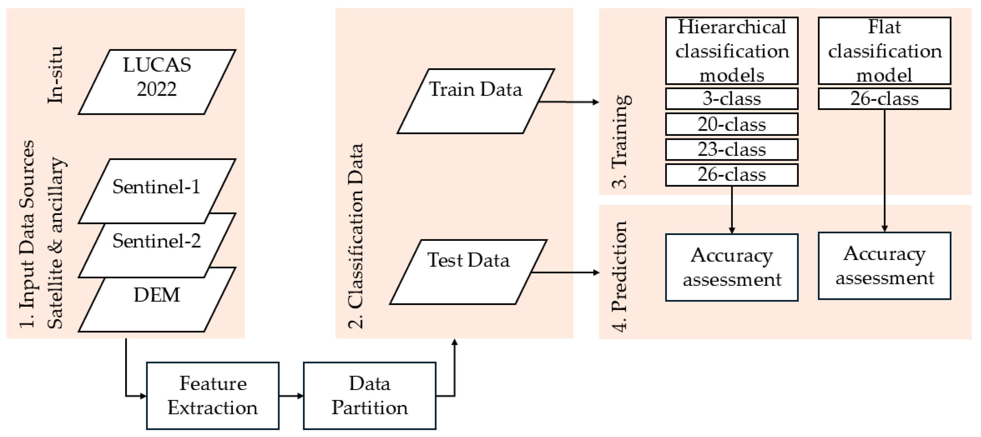
2.4. Classification Process

2.4.1. Classification Method

The Random Forest (RF) classifier was chosen for its strength, speed, and robustness in handling noisy data [47]. Introduced by Breiman, RF is known for its high classification accuracy and ability to quantify feature importance [48]. RF uses bagging (bootstrap + aggregation) to create an ensemble of decision trees. The algorithm trains using random subsets of samples and features in each decision tree instead of the entire dataset. A majority vote is used to combine the outputs of all trained trees, which helps to reduce variance and improve classification accuracy [49].
The RF classifier was configured with 140 trees, and the minimum number of samples at each leaf node was set to two. All other parameters were kept at their default settings. These choices were based on the successful performance of similar parameters in generating the previous EU-27 LULC map [12].
Both flat and hierarchical classifications are based on the RF algorithm. When applied to flat classification, the classification was performed in one step, treating all classes as equally distinctive. In contrast, in the hierarchical classification, we applied the RF algorithm sequentially: first to classify the broad Level-1 classes, and then to classify subcategories within the Level-1 classes. This tiered approach leveraged the robustness of the RF algorithm while managing class complexity.
A feature selection process was performed to optimize model efficiency. The classification and feature selection were conducted using the Scikit-learn package (Version: 1.3.2) in Python [50]. Features were selected based on their importance, as provided by the RF model, with only those exceeding their standard deviation retained for classification. As a result, the number of features was reduced from 1326 (including 242 from S2, 108 from S1, 960 from texture data, and 16 from auxiliary data) to 176. The utilized features are shown in Table S1.
Among the 176 important out of 1326 available features, 111 features belonged to S2 data, in which B11 and B12 bands were more effective than other spectral bands. Although most spectral features were useful, DIRESWIR, LAI, and LCCI were particularly influential. VH and DPSVIm had the most influence of all 39 essential S1 characteristics. Furthermore, all 14 texture features were obtained from S1 data, emphasizing the importance of radar data in texture-based discrimination. The remaining 12 were LST data demonstrating the significance of temperature data in LULC classification.

2.4.2. Train and Test Data

From the initial 137,966 LUCAS samples, 3753 were excluded because their Level-3 LC classes were missing or undefined. Next, Level-1 and Level-2 class labels were assigned based on Table 1 specifications. From the aforementioned EO data, 1326 features were extracted for the centroids of available 134,204 polygons out of 134,213. The dataset was refined to 121,229 samples, focusing only on vegetation classes within Level-1 LC (B—Cropland, C—Woodland, D—Shrubland, and E—Grassland) classes.
To establish both training and testing datasets, the samples underwent clustering using the K-means Lloyd method [51]. Spatial clustering enabled samples to be distributed across different zones of the EU-27 region by dividing them into 5 clusters. Within each cluster, samples were partitioned at the Level-3 stage into training and testing datasets in a ratio of 2/3 and 1/3, respectively. After merging these datasets, 81,101 samples were allocated to the training dataset and 40,114 samples to the testing dataset. Due to an insufficient number of subclass samples available, 84 samples were excluded from the process. Null values in samples were eliminated, thus reducing training and testing samples to 65,765 and 32,384, respectively.

2.4.3. Train Data Balancing

Apart from the centroid of the LUCAS Copernicus module polygon, data can also be derived from other points within these polygons. However, adding more samples could result in longer training times without necessarily improving classification accuracy [17]. Furthermore, extracting points from homogeneous polygons might result in redundant data, which can overfit the model performance.
In order to address the imbalanced distribution of classes in the training dataset, steps were taken to achieve a more balanced distribution of samples. To achieve this, the number of samples for underrepresented classes was increased by including additional samples from within the polygons in addition to those from the centroids.
The balancing procedure was applied at the Level-3 class stage. In classes with fewer than 1000 samples, if the total count of centroids and polygon samples remained below 1000, all samples from the polygons were included. Otherwise, the most dissimilar samples from the polygons were selected using a similarity measure to bring the total to 1000. This criterion was empirically defined to balance the class counts while avoiding oversampling.
The Euclidean Distance (ED) metric in feature space was used to measure similarities between samples within each polygon. Samples were sorted by their ED values (starting with the most dissimilar), and only a certain proportion of these were retained to ensure diversity.
This resulted in an increase from 65,765 to 90,361 training samples. Table 6 provides a detailed breakdown of the total available samples, initial samples, and balanced training samples for each Level-3 class.

3. Results

In order to evaluate the proposed classification workflows, 32,384 independent test samples were assessed using the confusion matrix (CM). Six assessment metrics were determined from the CM, including User’s Accuracy (UA), Producer’s Accuracy (PA), F1-score (a weighted average of UA and PA), Overall Accuracy (OA, which represents the number of correctly predicted samples compared to the total number of samples), and Kappa coefficient (K, a measure of how reliable the classification). The findings were examined using F1-scores and PA across individual classes, as well as OA and K. All results are provided in Tables S2 through S13. Each approach had various advantages and drawbacks depending on the class characteristics and sample size.
The study results led to refining the classification scheme up to P26. The balanced dataset was initially classified using 52 vegetation cover classes (P52) as a baseline, yielding an OA of 57.2% and K of 0.52 when applied to the balanced dataset. The hierarchical classification approach was then employed stepwise to reduce the number of classes at different phases (P3, P20, P22, P23, and P26), allowing gradual scheme refinement (see results in Table 7). The results are consistent with those reported in previous studies employing hierarchical classification methods. However, the smaller spatial extent of the study areas in earlier works contributed to their comparatively better results. As demonstrated in studies such as Balrriere et al. [52], which used a neural network, and Ratanopad Suwanlee et al. [53], which applied a RF classifier, classification performance tends to decrease as the scheme classification complexity is reduced. To assess how far the hierarchical approach improved the results, each classification level was compared to the original 52-class scheme.
Stopping at P26 was based on several considerations. As the classification scheme became more refined, particularly for the categories of Orchards, Groves, Woodland, and Grassland, high uncertainty among these classes presented a significant challenge. Because their spatial and spectral characteristics overlapped substantially, the model was restricted in producing meaningful separations and resulted in diminishing returns to OA and K. With hierarchical classification at P26, 62.2% of OA was achieved, which was improved to 64.8% with flat classification on a balanced dataset, representing a significant improvement over the full P52 classification (OA = 57.2%). Figure 3 illustrates the trends in OA and K along the number of classes (P3–P52), showing that accuracy declines as complexity scheme increases. According to these results, the classification depth achieved at P26 provides a practical balance between detail and accuracy for LULC classification.
Considering these factors, we stopped and analyzed the results at P26 since further refinement beyond this point would not significantly improve classification accuracy. It provided a satisfactory classification scheme that enhanced the depth of vegetation cover mapping while maintaining meaningful accuracy. The classification experiment compared four alternative strategies, with a focus on hierarchical versus flat classification approaches, which were applied to both balanced and imbalanced datasets. Thereafter, an analysis based on class-specific performance was performed. Lastly, the advantages and disadvantages of each method were discussed. For convenience, F1-scores of each class calculated by flat and hierarchical classification on original and balanced data are displayed in Table 8, and F1-scores and PA of each class are compared for flat and hierarchical classification on balanced data in Table 9. The following analysis will be mainly based on those tables.

3.1. Overall Accuracy and Kappa Scores

Flat classification on balanced data had the greatest overall performance in terms of OA and K, with an OA of 64.8% and a K of 0.58. This strategy regularly generated high F1-scores, indicating that balancing the dataset increased the model’s ability to classify major and minor classes reliably. In contrast, the flat classification method on original (imbalanced) data achieved slightly lower OA (64.3%) and K (0.57). Clearly, this drop reflects the difficulties associated with working with imbalanced data, in which classes with fewer samples are frequently misclassified or underrepresented.
The hierarchical classification on balanced data had a slightly lower OA of 62.2% and a K of 0.56. Although it did not outperform the flat classification approach overall, it had certain strengths, especially in dealing with underrepresented classes. However, the hierarchical classification on imbalanced data achieved an OA of 63.3% and a K of 0.57. Although OA for the hierarchical method on balanced data was lower than for imbalanced data, the F1-scores within classes mainly performed better.

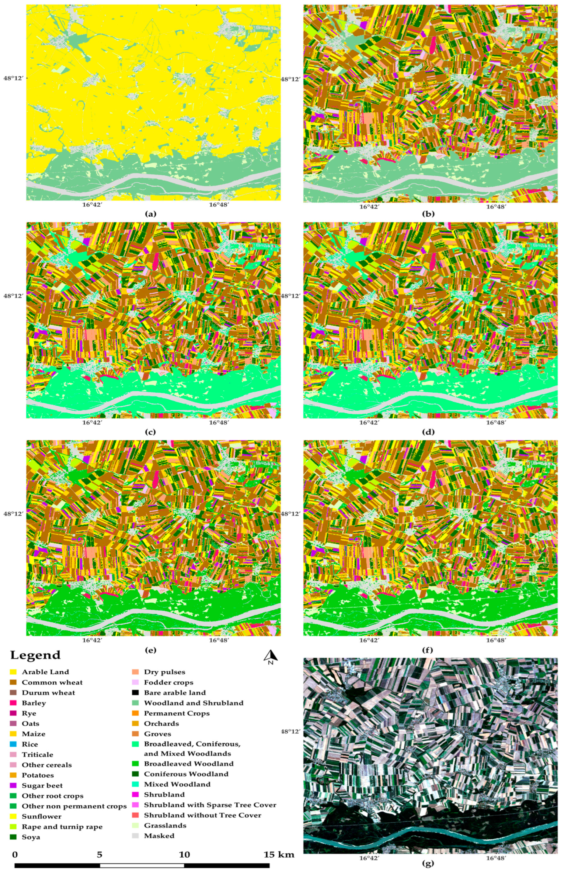
3.2. Visual Analysis of Classification Maps

Although the classification model is trained for EU27, for having a visual perspective, we mapped the LULC classification models across a 15 × 15 km subsection in the Marchfeld area near Vienna. Figure 4 presents these maps, revealing distinct spatial patterns among the schemes. In P3, the map shows large, uniform areas, suggesting broad categories with minimal differentiation. The P20 map introduces more varied patch sizes, which illustrates increased detail in LC types. Further fragmentation is evident in the P22 and P23 maps, showing smaller and more numerous patches that indicate progressive refinements in classification. The P26 hierarchical map displays some irregular patterns with jagged edges, implying challenges in delineating complex boundaries. In contrast, the P26 flat map presents smoother transitions between patches, suggesting improved consistency in spatial representation. It is worth noting that non-vegetation classes, including water bodies, settlements, and other non-vegetated areas, were masked using the CLCplus Backbone 2021 map (https://doi.org/10.2909/71fc9d1b-479f-4da1-aa66-662a2fff2cf7, accessed on 1 December 2024) in order to better focus the analysis on vegetation cover and enhance its relevance for agricultural and forest studies. While original S2 data provides a basic visual overview of the location, these maps illustrate the balance between thematic detail and spatial coherency.

3.3. Class-Specific Performance Analysis Based on F1-Scores

3.3.1. Large Sample Count Arable Land Classes

In the classes with a large test sample count (>1000), which includes Common wheat, Maize, and Barley, the classification performance exhibited a consistent trend across methods. For Common wheat, the flat classification on balanced data resulted in 70.2% of the F1-score, a little higher than the flat classification on original data, which scored 69.2%. Hierarchical methods produced similar results, scoring 70.0% for balanced data and 67.4% for original data. Hence, data balancing improved performance slightly, whereas the hierarchical approach did not enhance accuracy significantly.
Maize performed best with the flat classification based on balanced data, with an F1-score of 79.6%, followed closely by the flat classification based on original data, which scored 77.6%. Hierarchical classification on balanced data scored 77.7%, while hierarchical classification on original data received 74.6%. These findings show that, while hierarchical approaches perform relatively well, flat classification has a tiny advantage, particularly when the data is balanced.
Barley followed a similar trend, with the highest F1-score of 56.1% using a flat classification on balanced data, followed closely by 55.1% using a flat classification on original data. Hierarchical methods did not improve much, scoring 56.9% on balanced data and 54.9% on original data. Flat classification on balanced data appears to be the most effective method for large sample classes in Arable land.

3.3.2. Medium-Sample Arable Land Classes

In the medium sample category (test sample count between 200 and 1000), which includes crops like Durum wheat, Rape and turnip rape, Rye, Oats, Triticale, Sunflower, Fodder crops, and Soya, classification results varied across methods. Durum wheat achieved the highest F1-score with flat classification on balanced data (36.9%), surpassing the other approaches, particularly flat classification on original data (31.5%). Hierarchical techniques did not improve the outcomes, with 34.8% for balanced data and 33.0% for original data. In the case of Durum wheat, balancing the data enhances performance.
Rape and turnip rape performed well across all methods, with the highest F1-score of 76.8% for flat classification. Hierarchical approaches scored comparably well, ranging from 76.1% to 76.7%, indicating that all methods perform well for this crop and that other considerations, such as computation efficiency, may influence the choice of approach.
Rye and Oats displayed weaker results overall, with the flat classification on balanced data yielding the highest F1-scores at 37.9% for Rye and 30.7% for Oats. Hierarchical methods did not significantly improve performance, and only marginal gains were seen in some cases, like hierarchical classification on balanced data, which reached 39.4% for Rye.
Triticale fared badly across all techniques, with the maximum F1-score of 25.9% obtained using flat classification on balanced data, indicating a struggle in effectively classifying this crop.
For Sunflower, the flat classification of balanced data had an F1 score of 74.8%. In the hierarchical approaches, the Sunflower classification is slightly better (75.7% on balanced data), indicating its efficiency. Soya performed best using hierarchical classification on balanced data with an F1-score of 57.7%, which suggests that hierarchical methods might be helpful. Fodder crops only had moderate success, with the best result of 30.7% obtained from flat classification.

3.3.3. Small-Sample Arable Land Classes

For small sample classes (test sample count less than 200), including Potatoes, Other non-permanent industrial crops, Sugarbeet, Other root crops, and Other cereals, classification performance was highly variable, reflecting the difficulty of classifying small sample classes. Potatoes and Sugarbeet performed well in all methods tested. Sugarbeet received the greatest overall F1-score of 79.9% with flat classification on balanced data, followed by potatoes at 65.1%. Hierarchical approaches improved these crops slightly (80.6 and 65.3%, respectively).
Other non-permanent industrial crops and Other root crops had relatively low F1-scores due to classification challenges. Other non-permanent industrial crops had the finest performance with hierarchical classification on balanced data at 40.8%, whereas Other root crops performed poorly overall, with the highest score being 21.1% using the flat method. Similarly, Other cereals showed weak performance, with the best F1-score reaching 30.8% with flat classification on balanced data, reflecting the difficulty of accurately classifying small sample classes.
Rice, the smallest class, consistently performed poorly, with F1-scores of only 34.8% when employing hierarchical classification on balanced data. This shows that the small sample size makes any procedure difficult to perform satisfactorily. Hierarchical classification on balanced data seems to be an effective strategy for small sample classes on Arable land.

3.3.4. Permanent Crops and Orchards

The performance of permanent crops, such as Orchards and Groves, varied with their spectral complexity. For Orchards, all methods failed to achieve high accuracy, with F1-scores ranging from 8.2% to 25.6%. Although hierarchical classification is effective for heterogeneous classes, the results did not improve very much. A possible reason for this difficulty is that the spectral behaviors of Orchards and Other vegetation types are similar.
On the other hand, Groves performed better with an F1-score of 43.5% based on the hierarchical classification of the original data, indicating that this class has more distinguishable features, improving classification accuracy.

3.3.5. Grassland, Woodland, and Shrubland Classes

Woodland classes, including Broadleaved, Coniferous, and Mixed woodland, generally demonstrated a strong performance. The F1-scores for these classes were relatively high across all methods, indicating that they would be relatively easy to categorize. For example, Broadleaved woodland and Coniferous woodland achieved an F1-score of 71.3% and 73.5% using flat classification on balanced data, which indicates that flat classification methods may be sufficient for these well-defined groups. In addition, Mixed woodland performed well while utilizing this method, achieving an F1 score of 53.8%
Grassland performed well, with an F1-score of 72.8%, using hierarchical classification on original data. The results of this class were consistently positive, demonstrating that this class can be effectively classified with minimal impact on the selected method.
Shrubland classes, such as Shrubland with sparse tree cover and Shrubland without tree cover, were among the most challenging to classify. Shrubland with sparse tree cover achieved very low F1-scores across all methods, with a maximum of 12.6% using hierarchical classification on the original data. Because of its spectral similarity to other vegetation types, even hierarchical methods could not classify it accurately. In the Shrubland without tree cover classification, an F1-score of 32.8% was achieved, but it remained a challenging class overall.

3.4. Performance Based on Producer’s Accuracy

Upon comparing the flat and hierarchical methods based on balanced data, it becomes evident that the hierarchical approach frequently yields better PA results, particularly in more heterogeneous or less-represented classes.
For example, in large-sample Arable land classes such as Common wheat (75.1% PA in flat vs. 78.8% in hierarchical) and Maize (80.5% PA in flat vs. 83.4% in hierarchical), and in small-sample Arable Land classes like Durum wheat (30.3% PA in flat vs. 33.8% in hierarchical), Rice (20.0% PA in flat vs. 26.7% in hierarchical), and Soya (44.0% PA in flat vs. 48.0% in hierarchical), hierarchical classification consistently outperformed flat classification. Even in Woodland and Shrubland classes like Groves (34.3% PA in flat vs. 44.3% in hierarchical), Broadleaved woodland (77.3% PA in flat vs. 83.7% in hierarchical), and Shrubland without tree cover (20.4% PA in flat vs. 28.3% in hierarchical), hierarchical methods provided significant gains in PA.
Nevertheless, it must be noted that the hierarchical method does not consistently outperform the flat method. For Grassland, a class with a large number of samples (8589), the flat method achieved a higher PA of 83.1% compared to 62.0% with the hierarchical method. This suggests that the flat method can sometimes be more efficient for well-represented classes, as the complexity added by the hierarchical approach may not always be advantageous.

4. Discussion

This study investigated how deeply the original 52 vegetation cover classes can be explored using different classification schemes, aiming to increase classification thematic depth while maintaining meaningful accuracy across diverse LULC categories. This comprises LULC classifications based on EO data, including S1, and S2 satellite imagery, as well as auxiliary datasets such as LST and DEM. The RF classifier using both flat and hierarchical classification strategies was utilized to classify LC types across the EU, employing a balanced and imbalanced dataset for accuracy assessment. A suitable classification scheme was defined, and a hierarchical approach to classification was compared against flat classification methods concerning the level of LC detail at different levels.
Initially, classification on all 52 individual Level-3 classes led to low accuracy (OA = 57.2%, and K = 0.52) due to strong correlations among certain classes. Using trial and error, we refined our approach in order to explore how deeply and discriminatively we could classify the data. Nevertheless, as we advanced to the finer classification phases, the high correlation between classes limited the depth of separation, making it impossible to go further. We eventually settled on P26 with 26 classes, which partly made a trade-off between accuracy and discrimination.
The highest accuracy was obtained with a flat classification on balanced data (OA = 64.8% and K = 0.58), indicating that balancing the dataset was critical in enhancing model performance, particularly for underrepresented classes. Based on this finding, balanced datasets can improve classification results by addressing the underrepresentation of minority classes. Crops such as Maize and Durum wheat, for example, showed a gain in classification accuracy when their data was balanced, most likely because balancing allowed these smaller classes to be better represented in the dataset. Higher F1-scores across classes demonstrate the importance of balancing.
Although the flat classification method yielded the best overall results, the hierarchical classification approach demonstrated its value in handling heterogeneous and underrepresented classes. The flat classification method on balanced data showed strong F1-scores for several well-represented classes. For example, Maize achieved an F1-score of 79.6%, Common wheat reached 70.2%, and Grassland scored 72.7%. This shows the flat method’s ability to classify large, distinct classes with enough data representation efficiently. Other well-defined crops, such as Sugar beet (79.9%) and Rape and turnip rape (76.8%), also performed remarkably under the flat method. However, flat classification struggles with certain underrepresented or heterogeneous classes like Oats (30.7%) and Shrubland with sparse tree cover (9.2%). This indicates that the method’s simplicity is less successful in heterogeneous classes or with insufficient training data. The hierarchical classification strategy increased PA, especially for complicated or underrepresented classes. For example, Oats increased from 23.2% (flat) to 28.7% (hierarchical), Groves from 34.3% to 44.3%, and Rice from 20.0% to 26.7%. Even heterogeneous classes, such as Shrubland without tree cover, exhibited PA increases (from 20.4% to 28.3%). Despite this, hierarchical classification did not consistently increase F1-scores in all classes. Hierarchical techniques provided little improvement for well-defined crops such as Potatoes, Sugar beet, and Soya. Furthermore, the hierarchical technique performed poorly in the well-represented Grassland class, with PA decreasing from 83.1% to 62.0%.
Flat classification performed best on balanced data, particularly for large and medium arable land classes, resulting in higher F1-scores and OA for large sample classes like Maize and Common wheat compared to hierarchical methods. However, it struggled with imbalanced data, particularly for smaller or underrepresented classes, negatively impacting its performance. The model could focus on specific distinctions by dividing the classification process into phases.
Hierarchical techniques performed significantly better in terms of PA for most classes. The main disadvantage of hierarchical classification was a slight drop in OA and K, adding complexity that was not always necessary for well-represented classes, such as Grassland, where the flat method achieved a higher PA. While flat classification excels with balanced data and large classes, hierarchical classification is advantageous for smaller or more heterogeneous classes, particularly in PA. The choice of method should be based on class distribution and specific classification needs.
When comparing the two methods, flat classification outperforms the other for well-represented and distinct classes in terms of F1 scores. In contrast, hierarchical classification improves PA in complicated or underrepresented classes. Flat classification is suitable for big, well-defined classes where simplicity and OA are essential. Balancing the dataset remains critical in both techniques for improving performance across classes.

5. Conclusions

This work investigates how well different classification schemes can classify 52 vegetation cover classes, aiming to increase the classification depth and maintain desirous accuracy across various Land Use and Land Cover (LULC) categories. First, the approach extracted Earth Observation (EO) features, including Sentinel-1 and Sentinel-2 imagery, supplementary temperature, and elevation data for the European Land Use/Cover Area frame Survey (LUCAS) field dataset. The Random Forest classifier, later with flat and hierarchical classification strategies, was used for LULC classification across the European Union, refining the classification schemes and evaluating the impact of classification depth on accuracy, especially when using balanced and imbalanced datasets.
The results showed that the highest accuracy (overall accuracy (OA) = 64.8% and Kappa coefficient (K) = 0.58) was achieved with flat classification on balanced data, indicating the importance of addressing class imbalance to improve performance. Refining to 26 classes (P26) provided a practical balance, as accuracy declined with increasing detail (Figure 3). Increasing classification depth beyond this point did not yield significant improvements due to strong correlations among certain classes.
The flat classification method successfully provided higher F1-scores for well-represented classes such as Maize, Common wheat, and Grassland. Nevertheless, it struggled to deal with heterogeneous or underrepresented classes. The hierarchical classification achieved better producer’s accuracy (PA) in heterogeneous and underrepresented classes despite lower OA. Although high correlations between some classes hindered further refinement, hierarchical models dealt with class complexity effectively. Users can select between the faster, simpler flat classification method, which delivers better OA, and the hierarchical approach, which produces more precise results, notably in PA for challenging or underrepresented classes with higher processing demands. Decisions should be made based on particular applications, including large-scale monitoring, precision agriculture, forest management, or environmental protection.
To improve classification accuracy, we explored two additional experiments: incorporating training samples from LUCAS 2018 [54], selected based on class-specific sample counts, and evaluating phenological and productivity features from the HR-VPP dataset [55] in selected regions of Spain and Poland. Neither method significantly improved outcomes, probably due to existing limitations in LULC mapping, such as overlapping in spectral bands between vegetation types (for example, Grassland versus Woodland) and reliance on single-year data that does not fully consider the phenological variations. However, these experiments provide a basis for further research. It would be possible to capture temporal variability through a more comprehensive analysis that integrates multiple years of LUCAS data (2018 and 2022). In parallel, advanced deep learning techniques might better extract features, manage thematic complexity, and enhance accuracy and depth beyond the current 64.8% achieved OA at P26.

Supplementary Materials

The following supporting information can be downloaded at: https://www.mdpi.com/article/10.3390/rs17081379/s1.

Author Contributions

Conceptualization, all authors; methodology, B.G., E.I.-V. and F.V.; formal analysis, B.G.; writing—original draft preparation, B.G., E.I.-V. and F.V.; writing—review and editing, all authors; supervision, E.I.-V. and F.V. All authors have read and agreed to the published version of the manuscript.

Funding

This project was co-funded by the European Union’s Expert Contract No CT-EX2023D752321-101 under the EU Crop Map 2022—a 10 m crop type map of the EU based on the Earth Observation satellite and LUCAS Copernicus 2022. This research was also co-funded by the European Union’s Horizon Europe Research and Innovation Program under Grant Agreement No 101060423 LAMASUS project.

Data Availability Statement

The data supporting this study’s findings are available from the first author upon request.

Conflicts of Interest

The authors declare no conflicts of interest.

References

  1. European Commission: Joint Research Centre; Soille, P.; Lumnitz, S.; Albani, S. From Foresight to Impact. In Proceedings of the 2023 Conference on Big Data from Space (BiDS’23), Vienna, Austria, 6–9 November 2023; Publications Office of the European Union: Luxembourg, 2023. [Google Scholar]
  2. Common Agricultural Policy for 2023–2027. 28 CAP Strategic Plans at a Glance. Available online: https://agriculture.ec.europa.eu/document/download/a435881e-d02b-4b98-b718-104b5a30d1cf_en?filename=csp-at-a-glance-eu-countries_en.pdf (accessed on 23 November 2023).
  3. Sishodia, R.P.; Ray, R.L.; Singh, S.K. Applications of Remote Sensing in Precision Agriculture: A Review. Remote Sens. 2020, 12, 3136. [Google Scholar] [CrossRef]
  4. Machefer, M.; Zampieri, M.; van der Velde, M.; Dentener, F.; Claverie, M.; d’Andrimont, R. Earth Observation based multi-scale analysis of crop diversity in the European Union: First insights for agro-environmental policies. Agric. Ecosyst. Environ. 2024, 374, 109143. [Google Scholar] [CrossRef]
  5. Abdi, A.M.; Carrié, R.; Sidemo-Holm, W.; Cai, Z.; Boke-Olén, N.; Smith, H.G.; Eklundh, L.; Ekroos, J. Biodiversity decline with increasing crop productivity in agricultural fields revealed by satellite remote sensing. Ecol. Indic. 2021, 130, 108098. [Google Scholar] [CrossRef]
  6. Guilpart, N.; Bertin, I.; Valantin-Morison, M.; Barbu, C.M. How much agricultural land is there close to residential areas? An assessment at the national scale in France. Build. Environ. 2022, 226, 109662. [Google Scholar] [CrossRef]
  7. MohanRajan, S.N.; Loganathan, A.; Manoharan, P. Survey on Land Use/Land Cover (LU/LC) change analysis in remote sensing and GIS environment: Techniques and Challenges. Environ. Sci. Pollut. Res. Int. 2020, 27, 29900–29926. [Google Scholar] [CrossRef]
  8. Potapov, P.; Turubanova, S.; Hansen, M.C.; Tyukavina, A.; Zalles, V.; Khan, A.; Song, X.-P.; Pickens, A.; Shen, Q.; Cortez, J. Global maps of cropland extent and change show accelerated cropland expansion in the twenty-first century. Nat. Food 2022, 3, 19–28. [Google Scholar] [CrossRef]
  9. Chen, B.; Tu, Y.; An, J.; Wu, S.; Lin, C.; Gong, P. Quantification of losses in agriculture production in eastern Ukraine due to the Russia-Ukraine war. Commun. Earth Environ. 2024, 5, 336. [Google Scholar] [CrossRef]
  10. Panek-Chwastyk, E.; Dąbrowska-Zielińska, K.; Kluczek, M.; Markowska, A.; Woźniak, E.; Bartold, M.; Ruciński, M.; Wojtkowski, C.; Aleksandrowicz, S.; Gromny, E.; et al. Estimates of Crop Yield Anomalies for 2022 in Ukraine Based on Copernicus Sentinel-1, Sentinel-3 Satellite Data, and ERA-5 Agrometeorological Indicators. Sensors 2024, 24, 2257. [Google Scholar] [CrossRef]
  11. Gomes, V.; Queiroz, G.; Ferreira, K. An Overview of Platforms for Big Earth Observation Data Management and Analysis. Remote Sens. 2020, 12, 1253. [Google Scholar] [CrossRef]
  12. Ghassemi, B.; Izquierdo-Verdiguier, E.; Verhegghen, A.; Yordanov, M.; Lemoine, G.; Moreno Martínez, Á.; de Marchi, D.; van der Velde, M.; Vuolo, F.; d’Andrimont, R. European Union crop map 2022: Earth observation’s 10-meter dive into Europe’s crop tapestry. Sci. Data 2024, 11, 1048. [Google Scholar] [CrossRef]
  13. Zioti, F.; Ferreira, K.R.; Queiroz, G.R.; Neves, A.K.; Carlos, F.M.; Souza, F.C.; Santos, L.A.; Simoes, R.E. A platform for land use and land cover data integration and trajectory analysis. Int. J. Appl. Earth Obs. Geoinf. 2022, 106, 102655. [Google Scholar] [CrossRef]
  14. Gorelick, N.; Hancher, M.; Dixon, M.; Ilyushchenko, S.; Thau, D.; Moore, R. Google Earth Engine: Planetary-scale geospatial analysis for everyone. Remote Sens. Environ. 2017, 202, 18–27. [Google Scholar] [CrossRef]
  15. d’Andrimont, R.; Yordanov, M.; Martinez-Sanchez, L.; Eiselt, B.; Palmieri, A.; Dominici, P.; Gallego, J.; Reuter, H.I.; Joebges, C.; Lemoine, G.; et al. Harmonised LUCAS in-situ land cover and use database for field surveys from 2006 to 2018 in the European Union. Sci. Data 2020, 7, 352. [Google Scholar] [CrossRef] [PubMed]
  16. d’Andrimont, R.; Verhegghen, A.; Lemoine, G.; Kempeneers, P.; Meroni, M.; van der Velde, M. From parcel to continental scale—A first European crop type map based on Sentinel-1 and LUCAS Copernicus in-situ observations. Remote Sens. Environ. 2021, 266, 112708. [Google Scholar] [CrossRef]
  17. Ghassemi, B.; Dujakovic, A.; Żółtak, M.; Immitzer, M.; Atzberger, C.; Vuolo, F. Designing a European-Wide Crop Type Mapping Approach Based on Machine Learning Algorithms Using LUCAS Field Survey and Sentinel-2 Data. Remote Sens. 2022, 14, 541. [Google Scholar] [CrossRef]
  18. Ghassemi, B.; Immitzer, M.; Atzberger, C.; Vuolo, F. Evaluation of Accuracy Enhancement in European-Wide Crop Type Mapping by Combining Optical and Microwave Time Series. Land 2022, 11, 1397. [Google Scholar] [CrossRef]
  19. Waśniewski, A.; Hościło, A.; Chmielewska, M. Can a Hierarchical Classification of Sentinel-2 Data Improve Land Cover Mapping? Remote Sens. 2022, 14, 989. [Google Scholar] [CrossRef]
  20. Avci, M.; Akyurek, Z. A Hierarchical Classificaton of Landsat Tm Imagery for Landcover Mapping. Geogr. Pannonica 2004, 22, 4087. [Google Scholar]
  21. Demirkan, D.Ç.; Koz, A.; Düzgün, H.Ş. Hierarchical classification of Sentinel 2-a images for land use and land cover mapping and its use for the CORINE system. J. Appl. Rem. Sens. 2020, 14, 026524. [Google Scholar] [CrossRef]
  22. Peña, J.; Gutiérrez, P.; Hervás-Martínez, C.; Six, J.; Plant, R.; López-Granados, F. Object-Based Image Classification of Summer Crops with Machine Learning Methods. Remote Sens. 2014, 6, 5019–5041. [Google Scholar] [CrossRef]
  23. Gavish, Y.; O’Connell, J.; Marsh, C.J.; Tarantino, C.; Blonda, P.; Tomaselli, V.; Kunin, W.E. Comparing the performance of flat and hierarchical Habitat/Land-Cover classification models in a NATURA 2000 site. ISPRS J. Photogramm. Remote Sens. 2018, 136, 1–12. [Google Scholar] [CrossRef]
  24. d’Andrimont, R.; Yordanov, M.; Sedano, F.; Verhegghen, A.; Strobl, P.; Zachariadis, S.; Camilleri, F.; Palmieri, A.; Eiselt, B.; Rubio Iglesias, J.M.; et al. Advancements in LUCAS Copernicus 2022: Enhancing Earth Observation with Comprehensive In-Situ Data on EU Land Cover and Use. Earth Syst. Sci. Data 2024, 16, 5723–5735. [Google Scholar] [CrossRef]
  25. European Commission, Joint Research Centre. LUCAS Copernicus 2022; European Commission, Joint Research Centre (JRC): Brussels, Belgium, 2023. [Google Scholar]
  26. Boegh, E.; Soegaard, H.; Broge, N.; Hasager, C.B.; Jensen, N.O.; Schelde, K.; Thomsen, A. Airborne multispectral data for quantifying leaf area index, nitrogen concentration, and photosynthetic efficiency in agriculture. Remote Sens. Environ. 2002, 81, 179–193. [Google Scholar] [CrossRef]
  27. JIANG, Z.; HUETE, A.; DIDAN, K.; MIURA, T. Development of a two-band enhanced vegetation index without a blue band. Remote Sens. Environ. 2008, 112, 3833–3845. [Google Scholar] [CrossRef]
  28. Pasqualotto, N.; Delegido, J.; van Wittenberghe, S.; Rinaldi, M.; Moreno, J. Multi-Crop Green LAI Estimation with a New Simple Sentinel-2 LAI Index (SeLI). Sensors 2019, 19, 904. [Google Scholar] [CrossRef] [PubMed]
  29. Wulf, H.; Stuhler, S. Sentinel-2: Land Cover, Preliminary User Feedback on Sentinel-2A Data. In Proceedings of the Sentinel-2A Expert Users Technical Meeting, Frascati, Italy, 29–30 September 2015. [Google Scholar]
  30. Kriegler, F.J.; Malila, W.A.; Nalepka, R.F.; Richardson, W. Preprocessing Transformations and Their Effects on Multispectral Recognition. In Proceedings of the Sixth International Symposium on Remote Sensing of Environment, Ann Arbor, MI, USA, 13–16 October 1969; Volume II, p. 97. [Google Scholar]
  31. Qi, J.; Chehbouni, A.; Huete, A.R.; Kerr, Y.H.; Sorooshian, S. A modified soil adjusted vegetation index. Remote Sens. Environ. 1994, 48, 119–126. [Google Scholar] [CrossRef]
  32. van Deventer, A.P.; Ward, A.D.; Gowda, P.H.; Lyon, J.G. Using thematic mapper data to identify contrasting soil plains and tillage practices. Photogramm. Eng. Remote Sens. 1997, 63, 87–93. [Google Scholar]
  33. Huete, A. A soil-adjusted vegetation index (SAVI). Remote Sens. Environ. 1988, 25, 295–309. [Google Scholar] [CrossRef]
  34. Bouhennache, R.; Bouden, T.; Taleb-Ahmed, A.; Cheddad, A. A new spectral index for the extraction of built-up land features from Landsat 8 satellite imagery. Geocarto Int. 2019, 34, 1531–1551. [Google Scholar] [CrossRef]
  35. Xu, H. Modification of normalised difference water index (NDWI) to enhance open water features in remotely sensed imagery. Int. J. Remote Sens. 2006, 27, 3025–3033. [Google Scholar] [CrossRef]
  36. Jacques, D.C.; Kergoat, L.; Hiernaux, P.; Mougin, E.; Defourny, P. Monitoring dry vegetation masses in semi-arid areas with MODIS SWIR bands. Remote Sens. Environ. 2014, 153, 40–49. [Google Scholar] [CrossRef]
  37. Blackburn, G.A. Quantifying Chlorophylls and Caroteniods at Leaf and Canopy Scales. Remote Sens. Environ. 1998, 66, 273–285. [Google Scholar] [CrossRef]
  38. dos Santos, E.P.; Da Silva, D.D.; do Amaral, C.H. Vegetation cover monitoring in tropical regions using SAR-C dual-polarization index: Seasonal and spatial influences. Int. J. Remote Sens. 2021, 42, 7581–7609. [Google Scholar] [CrossRef]
  39. Gini, R.; Sona, G.; Ronchetti, G.; Passoni, D.; Pinto, L. Improving Tree Species Classification Using UAS Multispectral Images and Texture Measures. IJGI 2018, 7, 315. [Google Scholar] [CrossRef]
  40. Conners, R.W.; Trivedi, M.M.; Harlow, C.A. Segmentation of a high-resolution urban scene using texture operators. Comput. Vis. Graph. Image Process. 1984, 25, 273–310. [Google Scholar] [CrossRef]
  41. Haralick, R.M.; Shanmugam, K.; Dinstein, I. Textural Features for Image Classification. IEEE Trans. Syst. Man. Cybern. 1973, 6, 610–621. [Google Scholar] [CrossRef]
  42. Chatziantoniou, A.; Psomiadis, E.; Petropoulos, G. Co-Orbital Sentinel 1 and 2 for LULC Mapping with Emphasis on Wetlands in a Mediterranean Setting Based on Machine Learning. Remote Sens. 2017, 9, 1259. [Google Scholar] [CrossRef]
  43. Mohammadpour, P.; Viegas, D.X.; Viegas, C. Vegetation Mapping with Random Forest Using Sentinel 2 and GLCM Texture Feature—A Case Study for Lousã Region, Portugal. Remote Sens. 2022, 14, 4585. [Google Scholar] [CrossRef]
  44. Nizalapur, V.; Vyas, A. Texture analysis for land use land cover (lulc) classification in parts of ahmedabad, gujarat. Int. Arch. Photogramm. Remote Sens. Spat. Inf. Sci. 2020, 43, 275–279. [Google Scholar] [CrossRef]
  45. Hulley, G.; Hook, S. MODIS/Terra Land Surface Temperature/3-Band Emissivity Monthly L3 Global 0.05Deg CMG V061; NASA EOSDIS Land Processes Distributed Active Archive Center: Sioux Falls, SD, USA, 2021.
  46. NASA/METI/AIST/Japan Space Systems, and U.S./Japan ASTER Science Team. ASTER Global Digital Elevation Model V003; LP DAAC: Sioux Falls, SD, USA, 2019. [CrossRef]
  47. Izquierdo-Verdiguier, E.; Zurita-Milla, R. An evaluation of Guided Regularized Random Forest for classification and regression tasks in remote sensing. Int. J. Appl. Earth Obs. Geoinf. 2020, 88, 102051. [Google Scholar] [CrossRef]
  48. Breiman, L. Random Forests. Mach. Learn. 2001, 45, 5–32. [Google Scholar] [CrossRef]
  49. Criminisi, A. Decision Forests: A Unified Framework for Classification, Regression, Density Estimation, Manifold Learning and Semi-Supervised Learning. FNT Comput. Graph. Vis. 2011, 7, 81–227. [Google Scholar] [CrossRef]
  50. Pedregosa, F.; Varoquaux, G.; Gramfort, A.; Michel, V.; Thirion, B.; Grisel, O.; Blondel, M.; Prettenhofer, P.; Weiss, R.; Dubourg, V.; et al. Scikit-learn: Machine Learning in Python. J. Mach. Learn. Res. 2011, 12, 2825–2830. [Google Scholar]
  51. Lloyd, S. Least squares quantization in PCM. IEEE Trans. Inform. Theory 1982, 28, 129–137. [Google Scholar] [CrossRef]
  52. Barriere, V.; Claverie, M.; Schneider, M.; Lemoine, G.; d’Andrimont, R. Boosting crop classification by hierarchically fusing satellite, rotational, and contextual data. Remote Sens. Environ. 2024, 305, 114110. [Google Scholar] [CrossRef]
  53. Ratanopad Suwanlee, S.; Keawsomsee, S.; Izquierdo-Verdiguier, E.; Som-Ard, J.; Moreno-Martinez, A.; Veerachit, V.; Polpinij, J.; Rattanasuteerakul, K. Mapping sugarcane plantations in Northeast Thailand using multi-temporal data from multi-sensors and machine-learning algorithms. Big Earth Data 2025, 1–30. [Google Scholar] [CrossRef]
  54. d’Andrimont, R.; Verhegghen, A.; Meroni, M.; Lemoine, G.; Strobl, P.; Eiselt, B.; Yordanov, M.; Martinez-Sanchez, L.; van der Velde, M. LUCAS Copernicus 2018: Earth-observation-relevant in situ data on land cover and use throughout the European Union. Earth Syst. Sci. Data 2021, 13, 1119–1133. [Google Scholar] [CrossRef]
  55. Copernicus Land Monitoring Service: High Resolution Vegetation Phenology and Productivity (Hr-Vpp), Seasonal Trajectories and VPP Parameters. Available online: https://land.copernicus.eu/en/technical-library/product-user-manual-of-seasonal-trajectories/@@download/file (accessed on 24 September 2024).
Figure 1. Study overview and main steps.
Remotesensing 17 01379 g001
Figure 2. Phase 3-3 (P26) classification scheme class distribution over EU-27.
Remotesensing 17 01379 g002
Figure 3. Overall Accuracy (OA, blue) and Kappa (K, orange) vs. classes (P3, P20, P22, P23, P26, P52) based on the balanced dataset (Table 7). P26 could represent a good trade-off between class details and classification accuracy.
Remotesensing 17 01379 g003
Figure 4. LULC classification maps for a 15 × 15 km Marchfeld area near Vienna for the year 2022. (a) P3 (3 classes), (b) P20 (20 classes), (c) P22 (22 classes), (d) P23 (23 classes), (e) P26 hierarchical (26 classes), (f) P26 flat (26 classes), (g) original Sentinel-2 data. Non-vegetation areas are masked.
Remotesensing 17 01379 g004
Table 1. The classification scheme contains three levels: Level-1 with four broad vegetation land cover classes, Level-2 with 20 classes, and Level-3 with 52 classes, correspondingly. Source: d’Andrimont et al. (2018) [16].
Level-1Level-2
EU-Map CodeEU-Map CodeClasses or CategoriesLevel-3 LUCAS Land Cover
200 Arable landSee below
211Common wheatB11—Common wheat
212Durum wheatB12—Durum wheat
213BarleyB13—Barley
214RyeB14—Rye
215OatsB15—Oats
216MaizeB16—Maize
217RiceB17—Rice
218TriticaleB18—Triticale
219Other cerealsB19—Other cereals
221PotatoesB21—Potatoes
222Sugar beetB22—Sugar beet
223Other root cropsB23—Other root crops
230Other non-permanent industrial cropsB34—Cotton | B35—Other fiber and oleaginous crops | B36—Tobacco | B37—Other non-permanent industrial crops
231SunflowerB31—Sunflower
232Rape and turnip rapeB32—Rape and turnip rape
233SoyaB33—Soya
240Dry pulses, vegetables, and
flowers
B41—Dry pulses | B42—Tomatoes | B43—Other fresh vegetables | B44—Floriculture and ornamental plants | B45—Strawberries
250Fodder cropsB51—Clovers | B52—Lucerne | B53—Other leguminous and mixtures for fodder | B54—Mixed cereals for fodder
300 Woodland and ShrublandB71—Apple fruit, B72—Pear fruit, B73—Cherry fruit, B74—Nuts trees, B75—Other fruit trees and berries, B76—Oranges, B77—Other citrus fruit | B81—Olive groves, B82—Vineyards, B83—Nurseries, B84—Permanent industrial crops | C10—Broadleaved woodland | C21—Spruce-dominated coniferous woodland | C22—Pine-dominated coniferous woodland | C23—Other coniferous woodland | C31—Spruce-dominated mixed woodland | C32—Pine-dominated mixed woodland | C33—Other mixed woodland | D10—Shrubland with sparse tree cover | D20—Shrubland without tree cover
500 GrasslandB55—Temporary grasslands | E10—Grassland with sparse tree/shrub cover | E20—Grassland without tree/shrub cover | E30—Spontaneously vegetated surfaces
Table 2. Assessed different hierarchical classification schemes. Please see Table 1 for details on the class code abbreviations.
P3P20P22P23P26
200211211211211 (B11)
212212212212 (B12)
213213213213 (B13)
214214214214 (B14)
215215215215 (B15)
216216216216 (B16)
217217217217 (B17)
218218218218 (B18)
219219219219 (B19)
221221221221 (B21)
222222222222 (B22)
223223223223 (B23)
230230230230 (B34 |B35 |B36 |B37)
231231231231 (B31)
232232232232 (B32)
233233233233 (B33)
240240240240 (B41 | B42 | B43 | B44 | B45)
250250250250 (B51 | B52 | B53 | B54)
300300B78B7B7 (B71 | B72 | B73 | B74 | B75 | B76 | B77)
B8B8 (B81 | B82 | B83 | B84)
C123C123C10
C20 (C21 | C22 | C23)
C30 (C31 | C32 | C33)
D12D12D10
D20
500500500500500 (B55 | E10 | E20 | E30)
Table 3. Utilized S2 extracted spectral bands and indices, as well as a biophysical parameter. [Notation: NIR = Near Infrared; SWIR = Shortwave Infrared].
Feature NameDescription
Spectral BandsB2: Blue (WL: 496.6 nm (S2A)/492.1 nm (S2B))
B3: Green (WL: 560 nm (S2A)/559 nm (S2B))
B4: Red (WL: 664.5 nm (S2A)/665 nm (S2B))
B5: Red Edge 1 (WL: 703.9 nm (S2A)/703.8 nm (S2B))
B6: Red Edge 2 (WL: 740.2 nm (S2A)/739.1 nm (S2B))
B7: Red Edge 3 (WL: 782.5 nm (S2A)/779.7 nm (S2B))
B8: NIR (WL: 835.1 nm (S2A)/833 nm (S2B))
B8A: NIR narrow (WL: 864.8 nm (S2A)/864 nm (S2B))
B11: SWIR 1 (WL: 1613.7 nm (S2A)/1610.4 nm (S2B))
B12: SWIR 2 (WL: 2202.4 nm (S2A)/2185.7 nm (S2B))
Spectral Indices and biophysical parameter BLFEI :   ( ( ( B 3 + B 4 + B 12 ) / 3 ) B 11 ) / ( ( ( B 3 + B 4 + B 12 ) / 3 ) + B 11 )
DIRESWIR :   B 4 B 11
EVI 2 :   ( ( B 8 B 4 ) ) / ( ( B 8 + B 4 + 1 ) ) 2.4
LAI :   3.618   ( 2.5     ( ( B 8 B 4 ) / ( B 8 + 6     B 4 7.5     B 2 + 1 ) ) ) 0.118
LAIg :   5.405   ( ( B 8 A B 5 ) / ( B 8 A + B 5 ) ) 0.114
LCCI :   B 7 / B 5
MNDWI :   ( ( B 3 B 11 ) ) / ( ( B 3 + B 11 ) )
MSAVI :   0.5     ( 2     B 8 + 1 s q r t ( ( 2     B 8 + 1 ) 2 8     ( B 8 B 4 ) ) )
NDBI :   ( ( B 11 B 8 ) ) / ( ( B 11 + B 8 ) )
NDTI :   ( ( B 11 B 12 ) ) / ( ( B 11 + B 12 ) )
NDVI :   ( ( B 8 B 4 ) ) / ( ( B 8 + B 4 ) )
SAVI :   ( ( B 8 B 4 ) ) / ( ( B 8 + B 4 + 0.5 ) ) 1.5
SRNIRR :   B 8 / B 4
Table 4. S1-derived microwave bands and indices.
Feature NameDescription
Microwave featuresVV: Single co-polarization, vertical transmit/vertical receive
VH: Dual-band cross-polarization, vertical transmit/horizontal receive
VV/VH: The ratio between the VV polarization and the VH polarization
DPSVIm : σ V V 0 σ V V 0 + σ V V 0 σ V H 0 2
Table 5. Utilized texture formulations and applications. [Notation: (i, j): row and column indices of the GLCM matrix. P(i, j): value at position (i, j) in the GLCM matrix. (μi, μj): mean values of i and j. (σi, σj): standard deviations of i and j. Ng: Number of gray levels.
Texture Feature NameFormulationApplication
Cont n = 0 N g 1 n 2 i = 1 N g j = 1 N g P ( i , j ) i j = n Analyzes the local variations in an image. Having a high contrast value indicates that there is a large difference between the intensities of neighboring pixels.
Corr i j i j P i , j μ i μ j σ i σ j Measures the linear relationship between pixel pairs. A higher correlation value means a more predictable texture.
Diss i , j = 0 N g 1 P i , j i j Calculates the average intensity difference between neighboring pixels. The greater the dissimilarity value, the greater the heterogeneity of the texture.
Ent i j P ( i , j )   l o g ( P ( i , j ) ) Measures image disorder or complexity. When the image is not texturally uniform, the entropy is large. The entropy of complex textures tends to be high.
IDM i j P i , j 1 + ( i j ) 2 Describes how close the GLCM distribution is to the GLCM diagonal. A high homogeneity value implies that elements are concentrated along the diagonal, inferring a more uniform texture.
Table 6. Available samples for classification at two classification levels: Level-1, with four broad vegetation LC classes, and Level-3, with 52 LC classes and their counts. The number of samples for initial and balanced training samples is included as well.
LUCAS Level-1 Land CoverLUCAS Level-3 Land CoverTotal Class CountInitial Training Sample CountBalanced Training Sample Count
B—CroplandB11—Common wheat814542114211
B12—Durum wheat9365761000
B13—Barley392921042104
B14—Rye10195501000
B15—Oats11535971000
B16—Maize633834193419
B17—Rice4427918
B18—Triticale10075161000
B19—Other cereals2171161000
B21—Potatoes7513811000
B22—Sugar beet7103411000
B23—Other root crops2331141000
B31—Sunflower15339011000
B32—Rape and turnip rape276714781478
B33—Soya4392541000
B34—Cotton143951000
B35—Other fiber and oleaginous crops
B36—Tobacco
B37—Other non—permanent industrial crops
4672291000
199335
99491000
B41—Dry pulses5583051000
B42—Tomatoes64401000
B43—Other fresh vegetables4352391000
B44—Floriculture and ornamental plants4621996
B45—Strawberries43211000
B51—Clovers3701821000
B52—Lucerne11016561000
B53—Other leguminous and mixtures for fodder7653831000
B54—Mixed cereals for fodder3732291000
B55—Temporary grasslands250913291329
B71—Apple fruit6513381000
B72—Pear fruit133671000
B73—Cherry fruit1851091000
B74—Nuts trees6734271000
B75—Other fruit trees and berries5143031000
B76—Oranges93601000
B77—Other citrus fruit5030955
B81—Olive groves158010431043
B82—Vineyards10686511000
B83—Nurseries73371000
B84—Permanent industrial crops97581000
C—Woodland C10—Broadleaved woodland22,61312,97812,978
C21—Spruce-dominated coniferous woodland384919451945
C22—Pine-dominated coniferous woodland510226422642
C23—Other coniferous woodland12786971000
C31—Spruce-dominated mixed woodland355818501850
C32—Pine-dominated mixed woodland266613181318
C33—Other mixed woodland244512881288
D—Shrubland D10—Shrubland with sparse tree cover383922632263
D20—Shrubland without tree cover378821912191
E—GrasslandE10—Grassland with sparse tree/shrub cover362321012101
E20—Grassland without tree/shrub cover22,49911,31611,316
E30—Spontaneously vegetated surfaces463926812681
Table 7. Classification results on defined hierarchical classification schemes based on the balanced dataset.
Classification PhaseOA and K for the Balanced Dataset
P384.3%, 0.75
P2076.5%, 0.66
P2269.2%, 0.61
P2369.0%, 0.61
P2662.2%, 0.56
P5257.2%, 0.52
Table 8. F1-scores of each class derived by flat and hierarchical classification on original and balanced data for P26.
Class NameLabelTest CountF1-Balance-FlatF1-Original-FlatF1-Balance-HierarchicalF1-Original-Hierarchical
Common wheat211209070.2%69.2%70.0%67.4%
Durum wheat21228436.9%31.5%34.8%33.0%
Barley213102856.1%55.1%56.9%54.9%
Rye21427337.9%27.6%39.4%36.8%
Oats21531030.7%24.1%34.7%24.9%
Maize216164179.6%77.6%77.7%74.6%
Rice2171528.6%0.0%34.8%0.0%
Triticale21826125.9%7.8%22.5%16.7%
Other cereals2196130.8%6.3%27.3%20.3%
Potatoes22118465.1%65.4%65.3%64.5%
Sugar beet22216979.9%79.5%80.6%81.7%
Other root crops2236421.1%5.9%20.5%5.9%
Other non-permanent industrial crops23018340.5%32.8%40.8%32.9%
Sunflower23144074.8%74.3%75.7%72.6%
Rape and turnip rape23274276.8%76.6%76.7%76.1%
Soya23312554.5%42.9%57.7%38.6%
Dry pulses, vegetables, and flowers24032241.8%33.9%34.6%38.6%
Fodder crops25070730.7%12.9%31.7%26.5%
Grassland500858972.7%71.8%70.9%72.8%
Orchards B763525.6%8.2%24.8%12.1%
Groves B889039.9%40.4%39.5%43.5%
Broadleaved woodlandC10638871.3%71.1%68.8%68.6%
Coniferous woodlandC20261173.5%73.7%73.5%73.1%
Mixed woodland C30218353.8%54.2%53.4%54.4%
Shrubland with sparse tree coverD1011059.2%11.1%10.5%12.6%
Shrubland without tree coverD20108428.0%27.4%32.6%32.8%
OA64.8%64.3%62.2%63.3%
K0.580.570.560.57
Table 9. PA of each class calculated by flat and hierarchical classification on balanced data in P26.
Class NameLabelTest CountPA-Balance-FlatPA-Balance-Hierarchical
Common wheat211209075.1%78.8%
Durum wheat21228430.3%33.8%
Barley213102854.5%57.8%
Rye21427329.7%34.1%
Oats21531023.2%28.7%
Maize216164180.5%83.4%
Rice2171520.0%26.7%
Triticale21826118.0%15.7%
Other cereals2196123.0%24.6%
Potatoes22118459.8%59.2%
Sugar beet22216978.7%78.7%
Other root crops2236412.5%12.5%
Other non-permanent industrial crops23018332.2%33.3%
Sunflower23144070.0%73.9%
Rape and turnip rape23274268.1%68.3%
Soya23312544.0%48.0%
Dry pulses, vegetables, and flowers24032247.2%50.6%
Fodder crops25070723.2%35.4%
Grassland500858983.1%62.0%
Orchards B763523.8%30.9%
Groves B889034.3%44.3%
Broadleaved woodlandC10638877.3%83.7%
Coniferous woodlandC20261173.0%74.1%
Mixed woodland C30218346.3%46.5%
Shrubland with sparse tree coverD1011055.2%6.4%
Shrubland without tree coverD20108420.4%28.3%
Disclaimer/Publisher’s Note: The statements, opinions and data contained in all publications are solely those of the individual author(s) and contributor(s) and not of MDPI and/or the editor(s). MDPI and/or the editor(s) disclaim responsibility for any injury to people or property resulting from any ideas, methods, instructions or products referred to in the content.

