Global Distribution and Local Variation of Pre-Rain Green-Up in Tropical Dryland

Abstract

Pre-rain green-up is a distinctive phenological phenomenon observed in arid and semi-arid regions, featuring the sprouting of plants before the onset of the rainy season. This phenomenon indicates the intricate controls of vegetation phenology other than precipitation, yet its global distribution patterns and underlying causes remain unclear. In this study, we used remotely sensed phenology and rainfall data to map the global distribution of pre-rain green-up vegetation for the first time in arid and semi-arid savanna areas. The results revealed that over one-third of pre-rain green-up vegetation is in mountainous regions. Furthermore, to explore the potential effect of groundwater accessibility on pre-rain green-up, we employed high-resolution imagery to quantify phenological parameters and analyzed the relationship between pre-rain green-up and elevation at the watershed scale in a typical mountainous pre-rain green-up region in Africa. We found that within the pre-rain green-up area, 60.64% of sub-watersheds show a significant negative correlation (p < 0.05) between the start of the season (SOS) and elevation, indicating that the SOS occurs earlier at higher elevations despite the complex spatial variability overall. Our study provides a global picture of the pre-rain green-up phenomenon in tropical drylands and suggests that tree internal water regulation mechanisms rather than groundwater accessibility control the pre-rain green-up.

1. Introduction

A unique phenological phenomenon known as pre-rain green-up, that is, vegetation green-up before the onset of the rainy season, has been observed in tropical semi-arid ecosystems where vegetation growth was thought to be driven by precipitation [1,2,3]. For instance, in the tropical eucalypt savannas of Australia, evergreen species exhibit leaf flushing throughout the dry season, while some semi-deciduous species display leaf flushing at the end of the dry season [4]. Similarly, in the dry monsoon forests of Thailand and India, new leaf growth occurs 1–2 months before the first monsoon rains [5]. In the savannas of Brazil and Africa, the greening and senescence of woody-dominated vegetation do not always align precisely with the onset and cessation of the rainy season [6,7].

The pre-rain green-up phenomenon reflects distinct vegetation responses to the timing of rainfall onset, which contradicts the precipitation-driven vegetation growth hypothesis. Therefore, understanding the mechanisms behind the pre-rain green-up phenomenon has noteworthy importance in the improvement of vegetation dynamics modeling [8,9]. One of the critical tasks is to map where pre-rain green-up is happening across global tropical savannas and woodlands characterized by the coexistence of grasses and trees with alternating dry and wet seasons [10], which has not yet been accomplished.

Woody and herbaceous plants interact by many mechanisms and maintain a competitive balance [11,12]. Savannas, as one of the valuable carbon sinks, holds the competitive balance between trees and grasses, with notable implications for primary productivity, carbon sequestration, and emissions dynamics [13,14]. The fractions of tree cover and grass cover in savannas are complementary, and a higher tree cover fraction potentially leads to more pronounced pre-rain green-up phenomena [15,16]. Conversely, areas with dominating herbaceous plants and lower tree cover fractions exhibit varying occurrences of pre-rain leaf flushing [17].

Current research is mostly conducted at species and plot scales [18,19] and regional scales [1,20], but few studies have explored the detailed global distribution of pre-rain green-up vegetation under different tree cover fractions in arid and semi-arid savannas. Research on hotspots of pre-rain green-up has relied mainly on moderate-resolution satellite imagery from MODIS [7,21]. Ryan [1] and Adole [7] used remote sensing observations to derive the spatial variation of the difference between vegetation green-up time and the start of the rainy season of different vegetation types in Africa at a 500 m resolution. Considering the scale effect of phenology, this could be not enough for investigating the spatial variation at the local scale of the phenomenon. To gain a more comprehensive understanding of the pre-rain green-up phenomenon, it is necessary to incorporate higher-resolution remote sensing data.

Besides the distribution, the mechanisms of pre-rain green-up are also under the veil. In the tropical savannas and woodlands, vegetation green-up is closely linked to photoperiod and precipitation patterns [22,23]. However, the occurrence of pre-rain green-up phenomena suggests that vegetation growth is not dependent on precipitation, implying that the water required for premature growth could possibly be sourced from deep soil water storage, accessed through deep roots [24,25]. Nevertheless, due to the coarse resolution of groundwater data, the hypothesis is yet to be verified.

The mountainous regions cover nearly one-third of the global land area. The distribution of heat and groundwater varies rapidly with elevation in the mountainous regions, creating a unique opportunity to study the cues of environmental impacts on vegetation phenological behaviors. We hypothesize that the distribution of groundwater is associated with elevation and will influence the extent of the pre-rain green-up phenomena. Therefore, we propose an investigation of pre-rain green-up in mountainous regions to delineate the detailed patterns and explore the underlying mechanisms of the phenomenon.

Overall, in this study, we aim to understand the large-scale distribution of pre-rain green-up and to investigate the relationship between the pre-rain green-up phenomenon and local scale topographical variation (as a proxy for groundwater accessibility), utilizing remote sensing earth observations of different scales and climate data. The specific research objectives are as follows:

• To describe the global distribution of the pre-rain green-up phenomenon by vegetation type and topography conditions using coarse-resolution imagery.
• To observe and compare the spring phenology of pre-rain green-up and post-rain green-up vegetation in mountainous regions at the small watershed scale and to analyze the relationship between spring phenology and elevation using high-resolution satellite data.
• To conduct regional-scale mapping and quantitative analysis of the aforementioned relationships.

2. Materials and Methods

2.1. Data

2.1.1. Phenology and Rainfall Data

The occurrence of pre-rain green-up in vegetation can be represented by the difference in days between the start of the growing season (SOS) and the start of the rainy season (SRS). Two sources of SOS were used in this study: Firstly, the ESA Copernicus Harmonized Sentinel-2 Level-2A (L2A) Collection was utilized to calculate the two-band enhanced vegetation index (EVI2) and to determine SOS. The L2A product provides atmospheric-corrected surface reflectance. Secondly, the MODIS phenology product (MCD12Q2) was employed in our study to explore the prevalence of pre-rain green-up in global savannas and to validate the results derived from Sentinel-2 observations. The onset of the growing season in the MODIS product was also derived from the EVI2 time series data [26].

For SRS estimates, we used Climate Hazards Group InfraRed Precipitation with Station data (CHIRPS), which were developed by the Climate Hazards Group at UCSB and scientists at the U.S. Geological Survey Earth Resources Observation and Science Center. It was proved to be more accurate in estimating the entire rainfall season cycle [27].

2.1.2. Land Cover and Topography Data

Two land cover products were adopted, which are the MCD12Q1 datasets of the International Geosphere-Biosphere Program (IGBP) classification and the European Space Agency (ESA) WorldCover 10 m 2020 product. Specifically, the former was utilized to delineate the global extent of savannas, while the latter was resampled to 30 m resolution and employed to determine the land cover types.

For topographic conditions, Sayre’s world mountain map was employed to determine the extent of mountainous regions [28]. Meanwhile, we used NASADEM in conjunction with sub-watershed delineations from HydroBASINS for the terrain analysis [29,30]. It is a reprocessed product of Shuttle Radar Topography Mission (SRTM) data [31]. Details of the above data are given in

Table 1. Dataset information for this study.

Datasets	Spatial Resolution	Time	References
Harmonized Sentinel-2 Level-2A Collection	10 m	2019–2020	ESA, 2020 [32]
MCD12Q1	500 m	2019	Sulla-Menashe & Friedl, 2018 [26]
MCD12Q2	500 m	2019–2020	Gray et al., 2019 [33]
CHIRPS	0.05°	2000–2020	Funk et al., 2015 [27]
ESA WorldCover product	10 m	2020	Zanaga et al., 2021 [34]
Sayre’s world mountain map	250 m	2018	Sayre et al., 2018 [28]
HydroBASINS	-	2013	Lehner & Grill, 2013 [29]
NASADEM	30 m	2019	Crippen et al., 2016 [30]

.

2.2. Study Area

We first selected savanna regions in arid and semi-arid areas, within the latitude range of 40°N to 40°S, to investigate the extension of the pre-rain green-up phenomenon on the whole globe in 2019 (Figure 1a). Savannas with tree cover ranging from 10 to 30% constitute 70.65% of the total study area, while woody savannas with tree cover ranging from 30 to 60% account for 29.35% of the total study area.

Further, we chose a mountain-concentrated area ranging from 2°S to 22°S and from 23°E to 41°E to explore the terrain effect on the phenomenon of pre-rain green-up (Figure 1b). The region exhibited evident pre-rain green-up with vast tropical and subtropical grasslands, savannas, and shrublands [35]. On topographic conditions, the region has elevations mainly varying from 300 to 1500 m and a wide range of low mountains and scattered low mountains, which account for 42 percent of the African mountainous area. Based on the topographic and hydrologic features, the region was divided into 6474 sub-watersheds in [data source].

2.3. Methods

2.3.1. Extraction of the Start of the Growing Season

At the global scale, we designated the date when EVI2 first surpassed 15% of the segment EVI2 amplitude as the start of the growing season (SOS) from MCD12Q2 [33]. Furthermore, by utilizing the NumCycles band of MCD12Q2, we excluded pixels with multiple growing seasons to maintain a one-to-one correspondence between growing and rainy seasons.

At the local scale, to extract higher-resolution SOS, we selected Sentinel-2 images in the blue, green, red, and near-infrared (NIR) bands of 10 m resolution to calculate EVI2 for time series reconstruction. Additionally, the scene classification (SCL) band was applied to mask pixels classified as cloud shadow, cloud, thin cirrus, water, and snow. Moreover, pixels with zero EVI2 observation for the two months from 1 December 2019 to 1 February 2020 were also filtered out to ensure at least one valid observation in cloudy summer weather, as they were found to affect the reconstruction of EVI2.

To mitigate the impact of missing values and noise, we employed the Harmonic Analysis of Time Series (HANTS) algorithm on Google Earth Engine (GEE) to reconstruct the EVI2 time series, which has been demonstrated to be a robust and effective method for reconstructing a wide range of time series data [36]. Following the reconstruction of the EVI2 time series, we applied a dynamic threshold approach to derive the vegetation phenological metric, SOS [37]. The method involved calculating the amplitude in the reconstructed EVI2 time series. A threshold value of 20% was selected [38,39], and SOS was subsequently defined as the date on which the reconstructed EVI2 time series reaches the minimum value plus 20% of the amplitude during the vegetation growth phase (Figure 2a). Given the study area’s location in the Southern Hemisphere and the fact that the vegetation phenology period transcends calendar years, we designated 1 June 2019 as the starting point for the annual cycle in our calculations, thereby establishing a consistent temporal reference frame for our analysis.

To minimize the influence of vegetation with two or more growing seasons in a year, a harmonic analysis was used to determine the number of seasons of the entire EVI2 time series [40]. We filtered pixels based on the amplitude ratio of the second to first harmonics, retaining only those with a ratio < 1, which corresponds to a single growing season pattern. Consistent with prior satellite-based phenology research, we masked sparse vegetation (i.e., annual mean EVI2 < 0.1) and weakly seasonal vegetation pixels (i.e., annual EVI2 amplitude < 0.1) [41]. In addition, we retained only the vegetation types relevant to our study, including trees (37.2% of all pixels), shrubs (33.37%), and grasses (16.38%), categorized in accordance with the ESA WorldCover map. Finally, we resampled the SOS image to a 30 m resolution to facilitate subsequent altitude analysis.

For the validation of the result, we compare the spatial consistency and details with MODIS products at the pixel scale. We randomly sampled 1,500,000 points within the study area and computed the correlation between the SOS calculated by GEE (GEE-SOS) and the MCD12Q2 product at woody vegetation pixel purity ratios of 0.9, 0.8, and 0.7. The GEE-SOS showed good agreement (R > 0.5) with the MCD12Q2 product. Furthermore, a higher purity ratio results in greater consistency between the SOS results and the MCD12Q2 product (Appendix A Figure A1).

2.3.2. Extraction of the Start of the Rainy Season

The Liebmann’s [42] method was used to determine the onset day of the rainy season in our study. The method, demonstrated to be effective in retrieving seasonal parameters of rainfall in tropical regions [43,44], is used to define the rainy season in a more objective and climate-based manner. It is divided into three steps.

Firstly, applying a harmonic analysis similar to that used for computing the vegetation SOS to remove pixels with multiple rainy seasons. Secondly, identifying the period of the year during which the rainy season typically occurs. This period is defined as the climatic water season. Specifically, the cumulative daily precipitation anomaly for the calendar year, C(d), was computed using the following formula:

$$\mathrm{C}\left(\mathrm{d}\right)={\sum }_{i=1Jan}^d{Q}_i-\overline{Q},$$

(1)

where $Q_i$ represents the climatological daily average of precipitation, where i goes from 1 January to 31 December and $\overline{Q}$ is the climatological annual-mean daily average precipitation. The date corresponding to the minimum value in C(d) denotes the onset of the climatic water season, indicating the day after which the daily precipitation exceeds the annual precipitation average. Conversely, the date corresponding to the maximum value in C(d) denotes the end of the climatic water season. Finally, the cumulative daily precipitation anomaly for the study year was calculated as the sum of the differences between daily precipitation and the climatological annual mean daily precipitation, over a period of 50 days preceding the start of the climatic water year to 50 days after the end of the climatic water year (Figure 2b). The date corresponding to the minimum value of the cumulative daily precipitation anomaly represents the start of the rainy season. In addition, the data were resampled to a spatial resolution of 500 m and 30 m using the nearest neighbor resampling method.

2.3.3. Covariation Between SOS and Elevation

We analyzed the spatial relationships between the SOS of the pre-rain green-up woody vegetation and elevation. Initially, a linear regression was performed on each sub-watershed. The slopes of the regression were then calculated to interpret the spatial relationships between SOS and elevation. A positive slope indicates a positive elevational gradient in phenology, where the SOS of vegetation is delayed with increasing altitudes. Conversely, a negative slope corresponds to a negative elevational gradient, where the SOS of vegetation is advanced with increasing altitudes. Then, a comparative analysis of elevation gradients in the SOS of pre-rain green-up woody vegetation and post-rain green-up woody vegetation was performed, providing further evidence to support the elevation-related feature of pre-rain green-up vegetation SOS.

We used the boxplot method to eliminate outliers of the SOS [45]. In each sub-watershed, the elevation range was restricted to 50–2000 m, where vegetation density is relatively high, and a minimum elevation difference of 50 m was required. After these filtering procedures, a minimum of 2000 valid pixels was required for each sub-watershed to ensure sufficient sample size for conducting the linear regression analysis.

3. Results

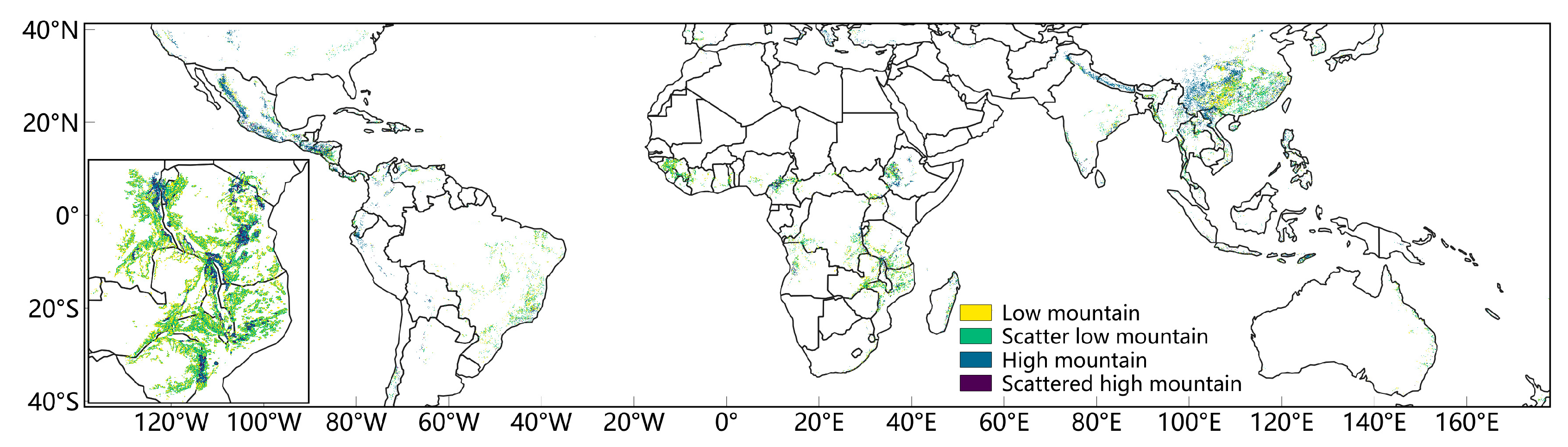
3.1. Spatial Distribution of the Pre-Rain Green-Up Phenomenon in the Mid to Low Latitudes

Across the arid and semi-arid savannas, pre-rain green-up vegetation was predominantly concentrated between the northern and southern 30° of latitudes, with notable hotspots in Africa, southern North America, southeastern Brazil, eastern India, northern Australia, and southern China. Africa accounted for the largest proportion of 47.04% of the global pre-rain green-up vegetation, followed by Brazil and China, which accounted for 13.34% and 12.11%, respectively (Figure 3a).

The distribution of this phenomenon was associated with vegetation type and topography. In the woody savannas, which occupy a smaller proportion (38.42%) of the study area, the proportion of pre-rain green-up vegetation with more than 30 days (66.54%) is higher (Figure 3b). More than one-third of the savannas exhibiting pre-rain green-up were located in mountainous regions (Appendix A Figure A2). Moreover, pre-rain green-up is more prevalent in low mountains and scattered low mountains, accounting for 65.07% of the phenomenon (Figure 3c).

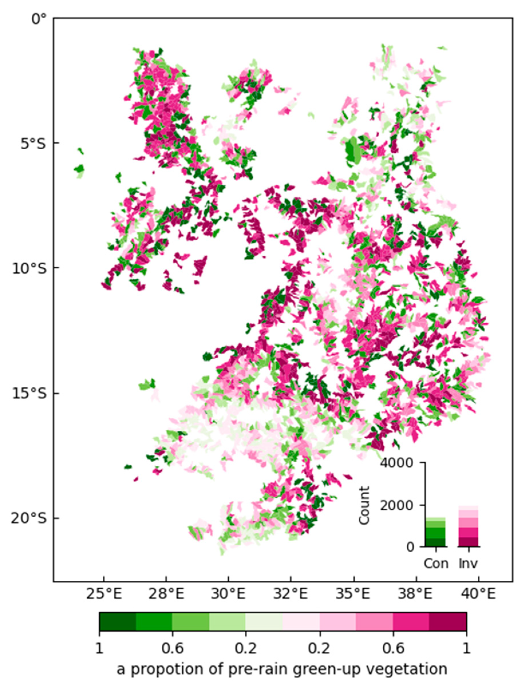
3.2. High-Resolution Mapping of the Pre-Rain Green-Up Phenomenon in African Mountainous Areas

The SOS demonstrated marked spatial heterogeneity across the study area, with earlier SOS in the Congo Basin (SOS c. 200) and later SOS in central Malawi (SOS > 350) (Figure 4a). The spatial distribution of the SRS exhibits a similar spatial pattern to that of the SOS (Figure 4b). The rainy season first fell on the Congo Basin (about 270 DOY on average) and then spread south-eastwards. Mozambique experienced the latest rainy season, with the SRS at around 350 DOY (Figure 4b).

The spatial patterns of SOS and pre-rain green-up exhibited distinct differences, and earlier vegetation growth did not necessarily imply the occurrence of pre-rain green-up. Regionally, the pre-rain green-up phenomenon was concentrated in the southern parts of the West Rift Valley Ranges and East Rift Valley Ranges, the eastern part of the Zambia Plateau, the northwestern and eastern parts of the Zimbabwe Plateau, the central and western parts of the Malawi Highlands, and the central part of the Central East Africa Plateau (Figure 4c). A substantial proportion (65%) of vegetation displayed an advance of more than 7 days between the SRS and the SOS, with distinct variations among different vegetation types (Figure 4c,e). Specifically, trees accounted for 52% of the total pre-rain green-up vegetation, with a concentrated difference of 8–33 days between the SRS and the SOS. Shrublands accounted for 30% of the total, with a concentrated difference of −5–17 days between the SRS and the SOS. In contrast, grasslands did not exhibit a significant pre-rain green-up phenomenon (Figure A3).

3.3. The SOS–Elevation Relationship of Pre-Rain Green-Up Areas

We characterized the effect of elevation on vegetation by a regression relationship between SOS and elevation. We chose three watersheds with a medium percentage of pre-rain green-up vegetation (about 50%) and examined the variations in SOS along the elevation gradient at the watershed scale by pre-rain and post-rain green-up groups (Figure 5a). The SOS and elevation for the three watersheds are detailed in Appendix A (Figure A4). In all three watersheds, the pre-rain green-up vegetation exhibited a negative correlation between the SOS and elevation (Figure 5b,d,f), which is noted as a negative elevational gradient in SOS. Contrarily, the post-rain green-up vegetation either showed a positive elevational gradient or had low significance in a negative trend between SOS and elevation (Figure 5c,e,g).

Extending to the entire region, we investigated the elevational gradients of SOS for pre-rain green-up vegetation in each sub-watershed. We found that in most sub-watersheds (60.64%), the pre-rain green-up vegetation showed a significant (p < 0.05) negative elevational gradient (Figure 6). Moreover, the sub-watersheds with a proportion of pre-rain green-up vegetation between 60 and 80% showed the most pronounced negative elevation gradient.

Further regional analysis revealed significant differences in the phenology–elevation relationships between pre-rain green-up vegetation and post-rain green-up vegetation. In 61.49% of the sub-watersheds, the elevational gradients for the two types of vegetation were inversed (Figure 7). Notably, 69.03% of the inversed cases were in the pattern that the SOS of pre-rain green-up vegetation showed a negative elevational gradient, while the SOS of post-rain green-up vegetation showed a positive elevational gradient. This inversed pattern was most pronounced in sub-watersheds with a proportion of pre-rain green-up vegetation between 60 and 80%.

4. Discussion

In this study, we explored the patterns of vegetation pre-rain green-up globally and in hotspot regions (Figure 3 and Figure 4). The results for pre-rain green-up vegetation distribution align with previous findings [46,47]. However, our analysis revealed that this phenomenon is more widespread globally than previously reported. Additionally, we quantitatively assessed the extent of pre-rain green-up across various mountain types and vegetation categories. Given the complexity of mountain microclimates, we investigated the impact of elevation on pre-rain green-up vegetation in mountain-rich regions of Africa (Figure 5 and Figure 6). Our findings indicate that pre-rain green-up vegetation is widespread in arid and semi-arid tropical savanna regions. At both global and local scales, pre-rain green-up vegetation exhibits a significantly inverse elevational gradient compared to post-rain green-up vegetation.

Numerous studies have explored the influence of elevation on the spatial variation of vegetation phenology [48,49,50,51], but investigations into the relationship between pre-rain green-up and African topography still need to be made available. Our study establishes a clear relationship between pre-rain green-up phenology and topographical factors, including elevation and regional terrain features. The inverse elevation gradient observed in pre-rain green-up phenology suggests that vegetation at higher elevations tends to initiate pre-rain leaf flushing earlier within the same sub-watershed. In most cases, vegetation spring phenology is delayed with increasing elevation due to temperature decreases. However, negative elevation gradients in vegetation phenology have also been documented. For instance, in a small valley in the United States, deciduous forest leaf-out at lower elevations occurred later, a phenomenon attributed to unique microclimatic conditions where cold air pooling led to lower temperatures at the valley bottom [52]. In arid and semi-arid regions, where sufficient thermal energy for vegetation growth is available, temperature is not the primary limiting factor for phenological responses to elevation. Instead, decreasing temperatures at higher elevations reduce evapotranspiration and carbon losses, making woody vegetation more prone to pre-rain leaf flushing. For example, in the Malawi-Lanwe mountains, the semi-evergreen ironwood A. johnsonii has been observed to leaf out by intercepting and absorbing humid air and light rainfall at higher altitudes [53]. In addition, the causes of this phenomenon also require consideration of soil moisture and soil texture. In the Luki Man and Biosphere Reserve of the Republic of Congo, the synergistic effects of oceanic influences and hilly topography create a microclimate characterized by elevated atmospheric humidity, even during the dry season, thereby facilitating new foliage production in trees [54]. Pre-rain green-up tends to occur preferentially in southern Africa on granitic substrates, whereas delayed greening is commonly observed on basaltic plains with heavier soils [53].

The drivers of the pre-rain green-up phenomenon remain uncertain. Some studies suggest that increasing temperature, increasing photoperiod, and decreasing atmospheric vapor pressure deficits (VPDs) may act as potential drivers of early greening [17,46,55,56,57]. Among these, the most widely accepted explanation for the pre-rain green-up phenomenon is temporal niche partitioning, whereby vegetation initiates early greening to reduce intra-species competition. Scholes and Walker [55] first proposed that trees avoid competition with grasses for water and nutrients by starting their growth before the onset of the growing season. The coexistence of grass and trees can lead to competition for water following the first rainfall, with grass typically having easier access to shallow soil moisture [58]. The degree of pre-rain green-up in savannas also varies with tree cover (Figure 3b). Here, we briefly examine the distribution of pre-rain green-up days at the different percentages of tree cover (Figure A5). When grass and trees are equally distributed in savannas, the competition for surface water between them may be more intense. The early green mechanism highlights the dependence of pre-rain green-up vegetation on groundwater. Our findings indirectly suggest that the relationship between groundwater depth and topography is not simply a linear positive correlation. Moreover, differences in the functional traits of woody vegetation, particularly rooting depth, influence water utilization strategies. Studies have shown that more drought-resistant species exhibit higher root water content in arid and semi-arid regions, with high xylem volume roots helping to mitigate water loss through evaporation [19,59]. Given the spatial heterogeneity of pre-rain green-up vegetation, further research on the spatial distribution of different species could enhance our understanding of this phenomenon by combining ground-based measurements with remote sensing data. Such studies could clarify how variations in rooting traits and groundwater availability shape the timing and extent of pre-rain leaf flushing across diverse landscapes.

We utilized Sentinel-2 imagery to calculate phenological parameters, which provided spatial patterns comparable to those derived from MODIS imagery used in previous studies [26]. However, the coarser resolution of MODIS imagery (250 m pixels) exacerbates the issue of mixed pixels in savanna regions, where shrubs, trees, and grasslands are interspersed, thereby increasing the ambiguity in distinguishing different types of pre-rain green-up vegetation [60]. In contrast, high-resolution satellite systems are more effective in retrieving detailed spatial patterns of vegetation phenology [61]. They can also be used to precisely identify the locations of early greening well-wooded stands within the tropical savanna landscapes of Africa, facilitating more localized investigations [62].

Compared to other arid and semi-arid ecosystems, the mechanisms of the savanna ecosystem are relatively complex [63]. It poses a challenge for improving the simulation of vegetation dynamics in the ecosystem and earth system models. Understanding the distribution of pre-rain green-up can aid in developing phenological mechanisms in global vegetation dynamic models. Additionally, we hope these results can be integrated with more detailed eco-physiological studies to enhance our understanding of the drivers of plant phenology and their spatial variability, thereby improving the accuracy of predictions regarding the potential impacts of global change on the structure and function of the biosphere. Our study highlights that the influence of terrain on the pre-rain green-up phenomenon in savannas cannot be neglected. Trees in South Africa have exhibited more frequent early green-up strategies, suggesting that the risks associated with early green-up may be lower in this region. As future rainfall patterns change, the ecology of early green-up vegetation will likely be disrupted [64]. Moreover, topography plays a role in influencing the resilience of vegetation to such disturbances [65]. To further investigate the resilience of early green-up vegetation, the impact of topography on the pre-rain green-up phenomenon must be considered.

5. Conclusions

This study elucidated the global distribution of pre-rain green-up vegetation in arid and semi-arid savannas using remote sensing phenological and rainfall data. We generated the first global map of the pre-rain green-up phenomenon and revealed its distribution on each non-polar continent. We proved the pre-rain green-up to be the most prevalent in Africa and noted a large portion (more than one-third) of mountainous regions for the phenomenon.

Furthermore, we try to dig deeper into the geological drivers behind pre-rain green-up on a finer scale. Based on the hypothesis that pre-rain green-up relies on the supply from groundwater, whose distribution is modulated by topography, high-resolution satellite data were employed to quantify vegetation phenology in a mountainous African region with typical pre-rain green-up, thereby examining the relationship between pre-rain green-up vegetation phenology and topography. Our findings indicate that the pre-rain green-up phenomenon is closely related to vegetation type and is subject to topographic control. Notably, the phenology of pre-rain green-up vegetation exhibits an inverse phenological gradient along elevation (60.64%), contrasting with the elevational gradient of post-rain green-up vegetation. Our findings may suggest that tree internal water regulation mechanisms rather than groundwater influenced by topography accessibility control the pre-rain green-up, which should be further investigated through, for example, more detailed tree species mapping and spatial distribution analysis.

References

1. Ryan, C.M.; Williams, M.; Grace, J.; Woollen, E.; Lehmann, C.E.R. Pre-rain Green-up Is Ubiquitous across Southern Tropical Africa: Implications for Temporal Niche Separation and Model Representation. New Phytol. 2017, 213, 625–633. [Google Scholar] [CrossRef]
2. Verger, A.; Filella, I.; Baret, F.; Peñuelas, J. Vegetation Baseline Phenology from Kilometric Global LAI Satellite Products. Remote Sens. Environ. 2016, 178, 1–14. [Google Scholar] [CrossRef]
3. Di Lucchio, L.M.; Fensholt, R.; Markussen, B.; Ræbild, A. Leaf Phenology of Thirteen African Origins of Baobab (Adansonia digitata (L.)) as Influenced by Daylength and Water Availability. Ecol. Evol. 2018, 8, 11261–11272. [Google Scholar] [CrossRef] [PubMed]
4. Williams, R.J.; Myers, B.A.; Muller, W.J.; Duff, G.A.; Eamus, D. Leaf phenology of woody species in a north Australian tropical savanna. Ecology 1997, 78, 2542–2558. [Google Scholar] [CrossRef]
5. Elliott, S.; Baker, P.J.; Borchert, R. Leaf Flushing during the Dry Season: The Paradox of Asian Monsoon Forests. Glob. Ecol. Biogeogr. 2006, 15, 248–257. [Google Scholar] [CrossRef]
6. Arantes, A.E.; Ferreira, L.G.; Coe, M.T. The Seasonal Carbon and Water Balances of the Cerrado Environment of Brazil: Past, Present, and Future Influences of Land Cover and Land Use. ISPRS J. Photogramm. Remote Sens. 2016, 117, 66–78. [Google Scholar] [CrossRef]
7. Adole, T.; Dash, J.; Atkinson, P.M. Large-Scale Prerain Vegetation Green-up across Africa. Glob. Chang. Biol. 2018, 24, 4054–4068. [Google Scholar] [CrossRef]
8. Chen, X.; Chen, W.; Xu, M. Remote-Sensing Monitoring of Postfire Vegetation Dynamics in the Greater Hinggan Mountain Range Based on Long Time-Series Data: Analysis of the Effects of Six Topographic and Climatic Factors. Remote Sens. 2022, 14, 2958. [Google Scholar] [CrossRef]
9. Afuye, G.A.; Kalumba, A.M.; Orimoloye, I.R. Characterisation of Vegetation Response to Climate Change: A Review. Sustainability 2021, 13, 7265. [Google Scholar] [CrossRef]
10. Wigley, B.J.; Coetsee, C.; February, E.C.; Dobelmann, S.; Higgins, S.I. Will Trees or Grasses Profit from Changing Rainfall Regimes in Savannas? New Phytol. 2024, 241, 2379–2394. [Google Scholar] [CrossRef]
11. Dohn, J.; Dembélé, F.; Karembé, M.; Moustakas, A.; Amévor, K.A.; Hanan, N.P. Tree Effects on Grass Growth in Savannas: Competition, Facilitation and the Stress-Gradient Hypothesis. J. Ecol. 2013, 101, 202–209. [Google Scholar] [CrossRef]
12. House, J.I.; Archer, S.; Breshears, D.D.; Scholes, R.J. NCEAS Tree–Grass Interactions Participants Conundrums in Mixed Woody–Herbaceous Plant Systems. J. Biogeogr. 2003, 30, 1763–1777. [Google Scholar] [CrossRef]
13. Dobson, A.; Hopcraft, G.; Mduma, S.; Ogutu, J.O.; Fryxell, J.; Anderson, T.M.; Archibald, S.; Lehmann, C.; Poole, J.; Caro, T.; et al. Savannas Are Vital but Overlooked Carbon Sinks. Science 2022, 375, 392. [Google Scholar] [CrossRef]
14. Zhou, Y.; Bomfim, B.; Bond, W.J.; Boutton, T.W.; Case, M.F.; Coetsee, C.; Davies, A.B.; February, E.C.; Gray, E.F.; Silva, L.C.R.; et al. Soil Carbon in Tropical Savannas Mostly Derived from Grasses. Nat. Geosci. 2023, 16, 710–716. [Google Scholar] [CrossRef]
15. Guan, K.; Wood, E.F.; Medvigy, D.; Kimball, J.; Pan, M.; Caylor, K.K.; Sheffield, J.; Xu, X.; Jones, M.O. Terrestrial Hydrological Controls on Land Surface Phenology of African Savannas and Woodlands. J. Geophys. Res. Biogeosciences 2014, 119, 1652–1669. [Google Scholar] [CrossRef]
16. Seghieri, J.; Do, F.C.; Devineau, J.-L.; Fournier, A.; Seghieri, J.; Do, F.C.; Devineau, J.-L.; Fournier, A. Phenology of Woody Species Along the Climatic Gradient in West Tropical Africa. In Phenology and Climate Change; IntechOpen: London, UK, 2012; ISBN 978-953-51-0336-3. [Google Scholar]
17. Whitecross, M.A.; Witkowski, E.T.F.; Archibald, S. Savanna Tree-Grass Interactions: A Phenological Investigation of Green-up in Relation to Water Availability over Three Seasons. South Afr. J. Bot. 2017, 108, 29–40. [Google Scholar] [CrossRef]
18. Venter, S.M.; Witkowski, E.T.F. Phenology, Flowering and Fruit-Set Patterns of Baobabs, Adansonia Digitata, in Southern Africa. For. Ecol. Manag. 2019, 453, 117593. [Google Scholar] [CrossRef]
19. Godlee, J.L.; Ryan, C.M.; Siampale, A.; Dexter, K.G. Tree Species Diversity Drives the Land Surface Phenology of Seasonally Dry Tropical Woodlands. J. Ecol. 2024, 112, 1978–1991. [Google Scholar] [CrossRef]
20. Adole, T.; Dash, J.; Atkinson, P.M. Characterising the Land Surface Phenology of Africa Using 500 m MODIS EVI. Appl. Geogr. 2018, 90, 187–199. [Google Scholar] [CrossRef]
21. Cizek, A.; Aplin, P.; Powell, I. Measuring the Timing of Woody Green-Up in African Savannas—Which Modis Data to Use? In Proceedings of the 2021 IEEE International Geoscience and Remote Sensing Symposium IGARSS, Brussels, Belgium, 11–16 July 2021; pp. 1398–1401. [Google Scholar]
22. Guan, K.; Good, S.P.; Caylor, K.K.; Medvigy, D.; Pan, M.; Wood, E.F.; Sato, H.; Biasutti, M.; Chen, M.; Ahlström, A.; et al. Simulated Sensitivity of African Terrestrial Ecosystem Photosynthesis to Rainfall Frequency, Intensity, and Rainy Season Length. Environ. Res. Lett. 2018, 13, 025013. [Google Scholar] [CrossRef]
23. Adole, T.; Dash, J.; Rodriguez-Galiano, V.; Atkinson, P.M. Photoperiod Controls Vegetation Phenology across Africa. Commun. Biol. 2019, 2, 391. [Google Scholar] [CrossRef] [PubMed]
24. Stocker, B.D.; Tumber-Dávila, S.J.; Konings, A.G.; Anderson, M.C.; Hain, C.; Jackson, R.B. Global Patterns of Water Storage in the Rooting Zones of Vegetation. Nat. Geosci. 2023, 16, 250–256. [Google Scholar] [CrossRef] [PubMed]
25. Li, H.; Si, B.; Ma, X.; Wu, P. Deep Soil Water Extraction by Apple Sequesters Organic Carbon via Root Biomass Rather than Altering Soil Organic Carbon Content. Sci. Total Environ. 2019, 670, 662–671. [Google Scholar] [CrossRef] [PubMed]
26. Sulla-Menashe, D.; Friedl, M.A. User Guide to Collection 6 MODIS Land Cover (MCD12Q1 and MCD12C1) Product; USGS: Reston, VA, USA, 2018. [Google Scholar]
27. Funk, C.; Peterson, P.; Landsfeld, M.; Pedreros, D.; Verdin, J.; Shukla, S.; Husak, G.; Rowland, J.; Harrison, L.; Hoell, A.; et al. The Climate Hazards Infrared Precipitation with Stations—A New Environmental Record for Monitoring Extremes. Sci. Data 2015, 2, 150066. [Google Scholar] [CrossRef]
28. Sayre, R.; Frye, C.; Karagulle, D.; Krauer, J.; Breyer, S.; Aniello, P.; Wright, D.J.; Payne, D.; Adler, C.; Warner, H.; et al. A New High-Resolution Map of World Mountains and an Online Tool for Visualizing and Comparing Characterizations of Global Mountain Distributions. Mt. Res. Dev. 2018, 38, 240–249. [Google Scholar] [CrossRef]
29. Lehner, B.; Grill, G. Global River Hydrography and Network Routing: Baseline Data and New Approaches to Study the World’s Large River Systems. Hydrol. Process. 2013, 27, 2171–2186. [Google Scholar] [CrossRef]
30. Crippen, R.; Buckley, S.; Agram, P.; Belz, E.; Gurrola, E.; Hensley, S.; Kobrick, M.; Lavalle, M.; Martin, J.; Neumann, M.; et al. Nasadem global elevation model: Methods and progress. Int. Arch. Photogramm. Remote Sens. Spat. Inf. Sci. 2016, 41, 125–128. [Google Scholar] [CrossRef]
31. Buckley, S.M.; Agram, P.S.; Belz, J.E.; Crippen, R.E.; Gurrola, E.M.; Hensley, S.; Kobrick, M.; Lavalle, M.; Martin, J.M.; Neumann, M.; et al. NASADEM: User Guide. 2020. Available online: https://lpdaac.usgs.gov/documents/592/NASADEM_User_Guide_V1.pdf (accessed on 1 September 2022).
32. ESA. Level-2A Algorithm Theoretical Basis Document; Remote Sensing Systems: Santa Rosa, CA, USA, 2021. [Google Scholar]
33. Gray, J.; Sulla-Menashe, D.; Friedl, M.A. User Guide to Collection 6 MODIS Land Cover Dynamics (MCD12Q2) Product; NASA EOSDIS Land Processes DAAC: Missoula, MT, USA, 2019. [Google Scholar]
34. Zanaga, D.; Van De Kerchove, R.; De Keersmaecker, W.; Souverijns, N.; Brockmann, C.; Quast, R.; Wevers, J.; Grosu, A.; Paccini, A.; Vergnaud, S.; et al. ESA WorldCover 10 m 2020 V100. 2021. Available online: https://pure.iiasa.ac.at/id/eprint/17832/ (accessed on 1 September 2022).
35. Campbell, J.T. Middle Passages: African American Journeys to Africa, 1787–2005; Penguin Books: New York, NY, USA, 2007; ISBN 978-0-14-311198-6. [Google Scholar]
36. Zhou, J.; Menenti, M.; Jia, L.; Gao, B.; Zhao, F.; Cui, Y.; Xiong, X.; Liu, X.; Li, D. A Scalable Software Package for Time Series Reconstruction of Remote Sensing Datasets on the Google Earth Engine Platform. Int. J. Digit. Earth 2023, 16, 988–1007. [Google Scholar] [CrossRef]
37. Jonsson, P.; Eklundh, L. Seasonality Extraction by Function Fitting to Time-Series of Satellite Sensor Data. IEEE Trans. Geosci. Remote Sens. 2002, 40, 1824–1832. [Google Scholar] [CrossRef]
38. Wang, L.; Tian, F.; Wang, Y.; Wu, Z.; Schurgers, G.; Fensholt, R. Acceleration of Global Vegetation Greenup from Combined Effects of Climate Change and Human Land Management. Glob. Chang. Biol. 2018, 24, 5484–5499. [Google Scholar] [CrossRef]
39. Jönsson, P.; Eklundh, L. TIMESAT—A Program for Analyzing Time-Series of Satellite Sensor Data. Comput. Geosci. 2004, 30, 833–845. [Google Scholar] [CrossRef]
40. Dunning, C.M.; Black, E.C.L.; Allan, R.P. The Onset and Cessation of Seasonal Rainfall over Africa. J. Geophys. Res. Atmos. 2016, 121, 11405–11424. [Google Scholar] [CrossRef]
41. Bolton, D.K.; Gray, J.M.; Melaas, E.K.; Moon, M.; Eklundh, L.; Friedl, M.A. Continental-Scale Land Surface Phenology from Harmonized Landsat 8 and Sentinel-2 Imagery. Remote Sens. Environ. 2020, 240, 111685. [Google Scholar] [CrossRef]
42. Liebmann, B.; Bladé, I.; Kiladis, G.N.; Carvalho, L.M.V.; Senay, G.B.; Allured, D.; Leroux, S.; Funk, C. Seasonality of African Precipitation from 1996 to 2009. J. Clim. 2012, 25, 4304–4322. [Google Scholar] [CrossRef]
43. Tian, J.; Luo, X.; Xu, H.; Green, J.K.; Tang, H.; Wu, J.; Piao, S. Slower Changes in Vegetation Phenology than Precipitation Seasonality in the Dry Tropics. Glob. Chang. Biol. 2024, 30, e17134. [Google Scholar] [CrossRef]
44. Dunning, C.M.; Black, E.; Allan, R.P. Later Wet Seasons with More Intense Rainfall over Africa under Future Climate Change. J. Clim. 2018, 31, 9719–9738. [Google Scholar] [CrossRef]
45. Ding, C.; Li, Y.; Xie, Q.; Li, H.; Zhang, B. Impacts of Terrain on Land Surface Phenology Derived from Harmonized Landsat 8 and Sentinel-2 in the Tianshan Mountains, China. GIScience Remote Sens. 2023, 60, 2242621. [Google Scholar] [CrossRef]
46. Higgins, S.I.; Delgado-Cartay, M.D.; February, E.C.; Combrink, H.J. Is There a Temporal Niche Separation in the Leaf Phenology of Savanna Trees and Grasses? J. Biogeogr. 2011, 38, 2165–2175. [Google Scholar] [CrossRef]
47. Yan, D.; Zhang, X.; Yu, Y.; Guo, W. Characterizing Land Cover Impacts on the Responses of Land Surface Phenology to the Rainy Season in the Congo Basin. Remote Sens. 2017, 9, 461. [Google Scholar] [CrossRef]
48. Gao, M.; Piao, S.; Chen, A.; Yang, H.; Liu, Q.; Fu, Y.H.; Janssens, I.A. Divergent Changes in the Elevational Gradient of Vegetation Activities over the Last 30 Years. Nat. Commun. 2019, 10, 2970. [Google Scholar] [CrossRef]
49. An, S.; Zhang, X.; Chen, X.; Yan, D.; Henebry, G.M. An Exploration of Terrain Effects on Land Surface Phenology across the Qinghai–Tibet Plateau Using Landsat ETM+ and OLI Data. Remote Sens. 2018, 10, 1069. [Google Scholar] [CrossRef]
50. Hua, X.; Ohlemüller, R.; Sirguey, P. Differential Effects of Topography on the Timing of the Growing Season in Mountainous Grassland Ecosystems. Environ. Adv. 2022, 8, 100234. [Google Scholar] [CrossRef]
51. Ding, C.; Huang, W.; Liu, M.; Zhao, S. Change in the Elevational Pattern of Vegetation Greenup Date across the Tianshan Mountains in Central Asia during 2001–2020. Ecol. Indic. 2022, 136, 108684. [Google Scholar] [CrossRef]
52. Fisher, J.; Mustard, J.; Vadeboncoeur, M. Green Leaf Phenology at Landsat Resolution: Scaling from the Field to the Satellite. Remote Sens. Environ. 2006, 100, 265–279. [Google Scholar] [CrossRef]
53. Cizek, A.F. Complex Spatial Patterns of Leaf Phenology within Semi-arid African Savanna Landscapes Driven by Rainfall and Topo-edaphic Variation Revealed Using Satellite Remote Sensing; Edge Hill University: Ormskirk, UK, 2024. [Google Scholar]
54. Angoboy Ilondea, B.; Beeckman, H.; Van Acker, J.; Van Den Bulcke, J.; Fayolle, A.; Couralet, C.; Hubau, W.; Kafuti, C.; Rousseau, M.; Kaka di-Makwala, A.; et al. Variation in Onset of Leaf Unfolding and Wood Formation in a Central African Tropical Tree Species. Front. For. Glob. Chang. 2021, 4, 673575. [Google Scholar] [CrossRef]
55. Scholes, R.J.; Walker, B.H. An African Savanna: Synthesis of the Nylsvley Study, 1st ed.; Cambridge University Press: Cambridge, UK, 1993; ISBN 978-0-521-41971-0. [Google Scholar]
56. Archibald, S.; Scholes, R.J. Leaf Green-up in a Semi-Arid African Savanna -Separating Tree and Grass Responses to Environmental Cues. J. Veg. Sci. 2007, 18, 583–594. [Google Scholar] [CrossRef]
57. Do, F.C.; Goudiaby, V.A.; Gimenez, O.; Diagne, A.L.; Diouf, M.; Rocheteau, A.; Akpo, L.E. Environmental Influence on Canopy Phenology in the Dry Tropics. For. Ecol. Manag. 2005, 215, 319–328. [Google Scholar] [CrossRef]
58. Bond, W.J. What Limits Trees in C4 Grasslands and Savannas? Annu. Rev. Ecol. Evol. Syst. 2008, 39, 641–659. [Google Scholar] [CrossRef]
59. Zhou, Y.; Wigley, B.J.; Case, M.F.; Coetsee, C.; Staver, A.C. Rooting Depth as a Key Woody Functional Trait in Savannas. New Phytol. 2020, 227, 1350–1361. [Google Scholar] [CrossRef]
60. Cheng, Y.; Vrieling, A.; Fava, F.; Meroni, M.; Marshall, M.; Gachoki, S. Phenology of Short Vegetation Cycles in a Kenyan Rangeland from PlanetScope and Sentinel-2. Remote Sens. Environ. 2020, 248, 112004. [Google Scholar] [CrossRef]
61. Tian, F.; Cai, Z.; Jin, H.; Hufkens, K.; Scheifinger, H.; Tagesson, T.; Smets, B.; Van Hoolst, R.; Bonte, K.; Ivits, E.; et al. Calibrating Vegetation Phenology from Sentinel-2 Using Eddy Covariance, PhenoCam, and PEP725 Networks across Europe. Remote Sens. Environ. 2021, 260, 112456. [Google Scholar] [CrossRef]
62. Abdi, A.M.; Brandt, M.; Abel, C.; Fensholt, R. Satellite Remote Sensing of Savannas: Current Status and Emerging Opportunities. J. Remote Sens. 2022, 2022. [Google Scholar] [CrossRef]
63. Haverd, V.; Smith, B.; Raupach, M.; Briggs, P.; Nieradzik, L.; Beringer, J.; Hutley, L.; Trudinger, C.M.; Cleverly, J. Coupling Carbon Allocation with Leaf and Root Phenology Predicts Tree–Grass Partitioning along a Savanna Rainfall Gradient. Biogeosciences 2016, 13, 761–779. [Google Scholar] [CrossRef]
64. Whitecross, M.A.; Witkowski, E.T.F.; Archibald, S. Assessing the Frequency and Drivers of Early-greening in Broad-leaved Woodlands along a Latitudinal Gradient in Southern Africa. Austral Ecol. 2017, 42, 341–353. [Google Scholar] [CrossRef]
65. Sang, Y.; Tian, F.; Jin, H.; Cai, Z.; Feng, L.; Dou, Y.; Eklundh, L. Assessing Topographic Effects on Forest Responses to Drought with Multiple Seasonal Metrics from Sentinel-2. Int. J. Appl. Earth Obs. Geoinf. 2024, 128, 103789. [Google Scholar] [CrossRef]
Figure 1. (a) Global distribution of savannas in arid and semi-arid regions (b) Location of sub-watersheds over the study region and (c) spatial distribution of elevation.
Remotesensing 17 01377 g001
Figure 2. The concept diagrams illustrating the extraction of parameters: (a) the start of the growing season (SOS); (b) the start of the rainy season (SRS) for a specific pixel (central coordinate: 35.61°E, 3.17°S). DOY, day of the year.
Remotesensing 17 01377 g002
Figure 3. Spatial distribution of the pre-rain green-up phenomenon in the mid to low latitudes. The pre-rain green-up phenomenon is indicated by the number of days that the start of growing season precedes the start of the rainy season. (a) Spatial distribution of the pre-rain green-up phenomenon. Pre-rain green-up hotspots are demarcated by the red boxes. (b) Variations in pre-rain green-up days among diverse savanna ecosystems. (c) Variations in pre-rain green-up days by mountain type.
Remotesensing 17 01377 g003
Figure 4. The spatial distribution of (a) SOS, (b) SRS, (c) pre-rain green-up phenomenon, (d) elevation, and (e) land cover map in the research region.
Remotesensing 17 01377 g004
Figure 5. (a) Three sub-watersheds were randomly selected across the research area, located in the east (I), south (II), and west (III) of the region. (b,d,f) The elevational gradients of SOS for pre-rain green-up vegetation in each sub-watershed. (c,e,g) The elevational gradients of SOS for post-rain green-up vegetation in each sub-watershed.
Remotesensing 17 01377 g005
Figure 6. The elevation gradients for pre-rain green-up vegetation. The color scheme employed here denotes elevation gradients, with purple indicating a negative trend and green signifying a positive trend. The gradual color transition from light to dark represents a proportion of pre-rain green-up vegetation, categorized into five distinct ranges: 0–0.2, 0.2–0.4, 0.4–0.6, 0.6–0.8, and 0.8–1.
Remotesensing 17 01377 g006
Figure 7. The relative relationship between elevation gradients of pre-rain green-up vegetation and post-rain green-up vegetation. Purple indicates an inverse elevation gradient between the two vegetation types, while green indicates a consistent elevation gradient. The transition from light to dark colors has the same meaning as in Figure 6.
Remotesensing 17 01377 g007