
Detecting Flooded Areas Using Sentinel-1 SAR Imagery


Abstract
1. Introduction
2. Methodology
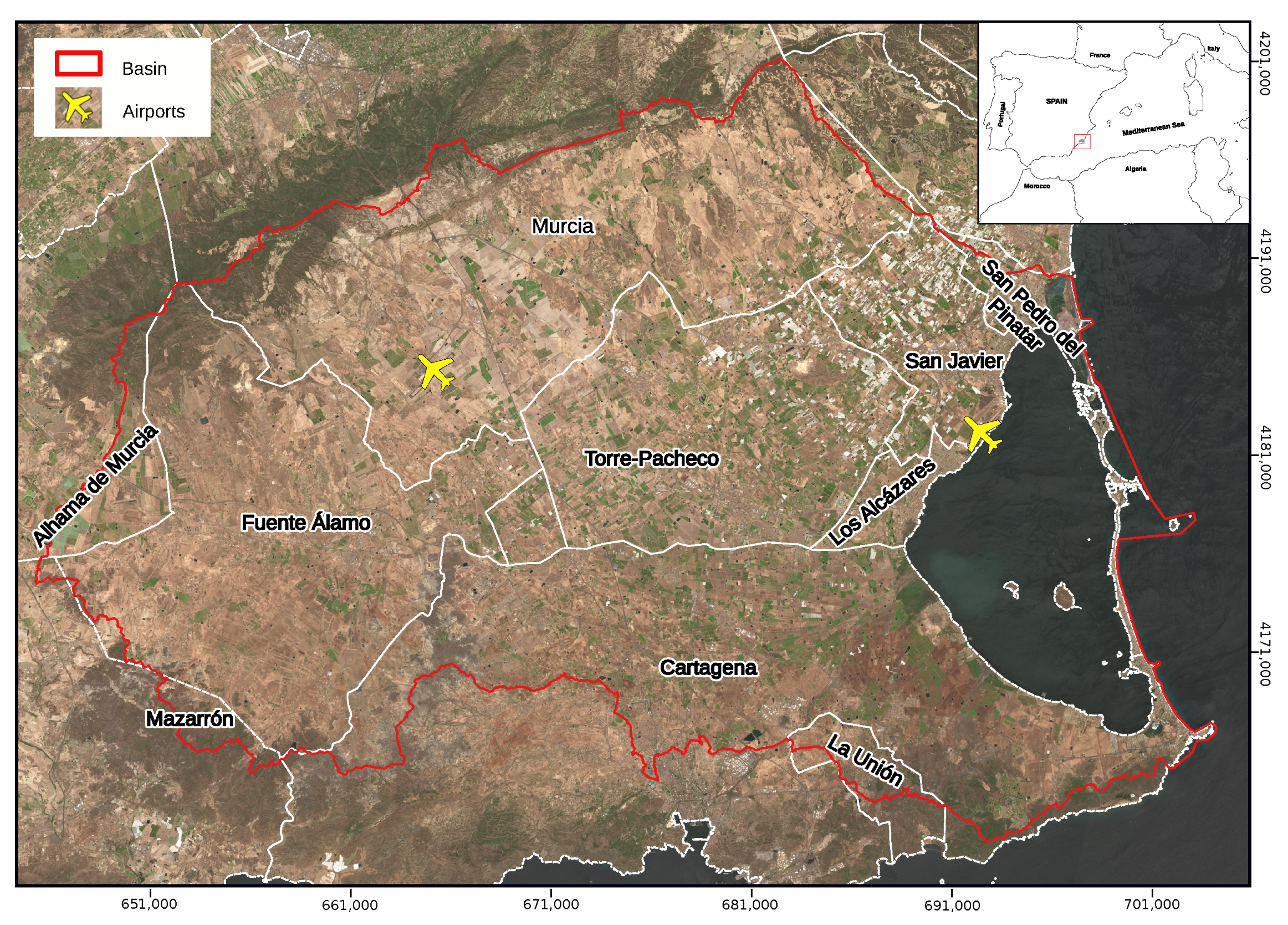
2.1. Study Area
2.2. Data
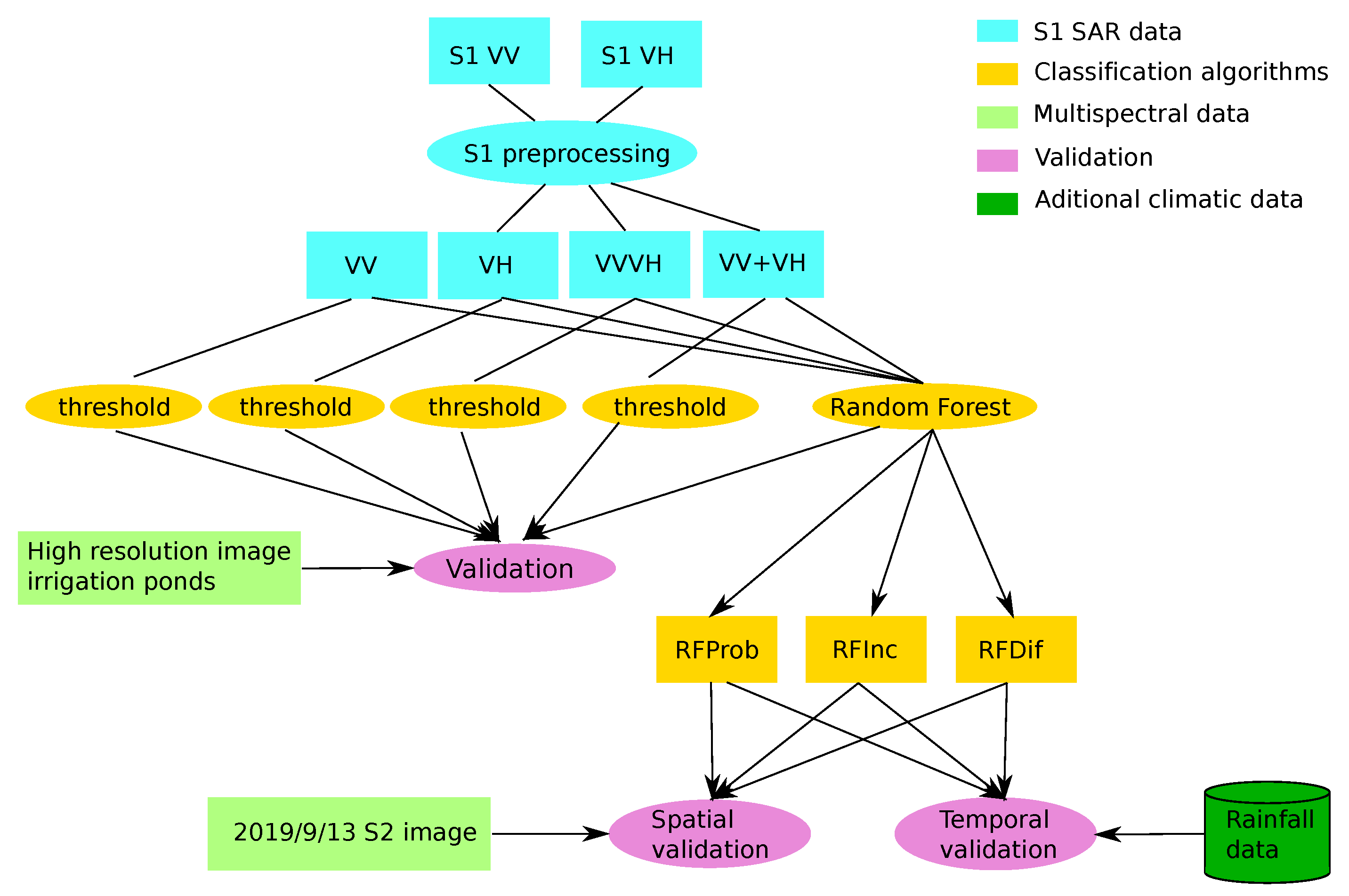
2.3. Algorithms
2.3.1. Thresholding
2.3.2. Random Forest Classification
2.3.3. Detection of Permanent Water Bodies and Infrastructures
2.3.4. Change Detection
- Calculate the increase in probability from an image previous to the event as where P is the probability of water presence after the event and is the probability of water presence before the event.
- Compute the difference in probability of water presence in two consecutive images before the event, compute the empirical distribution function of the differences (EDFp), and compute the p-value of the probability difference before and after the event for each pixel in the study area.
2.3.5. Slope Correction
2.4. Validation
3. Results
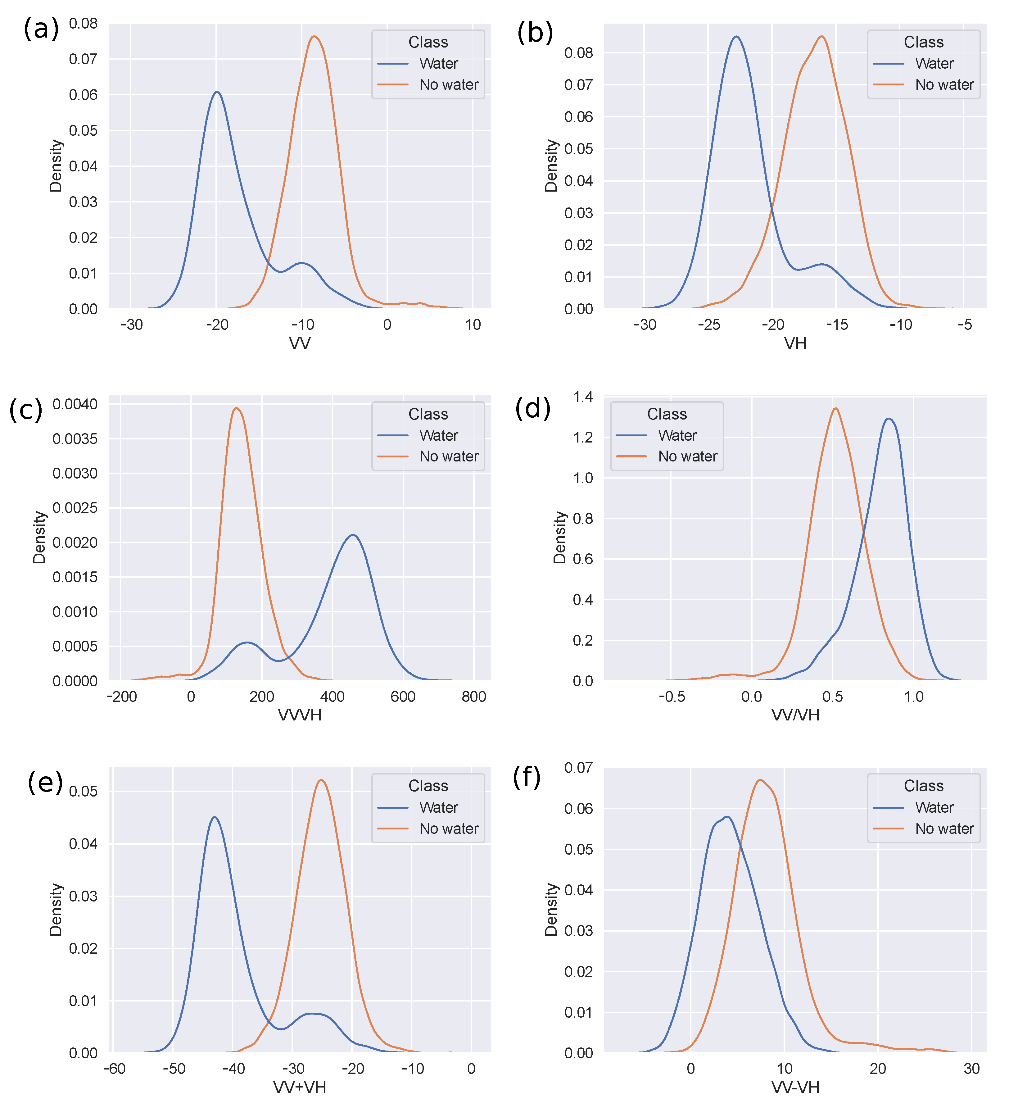
3.1. Thresholding
3.2. Classification
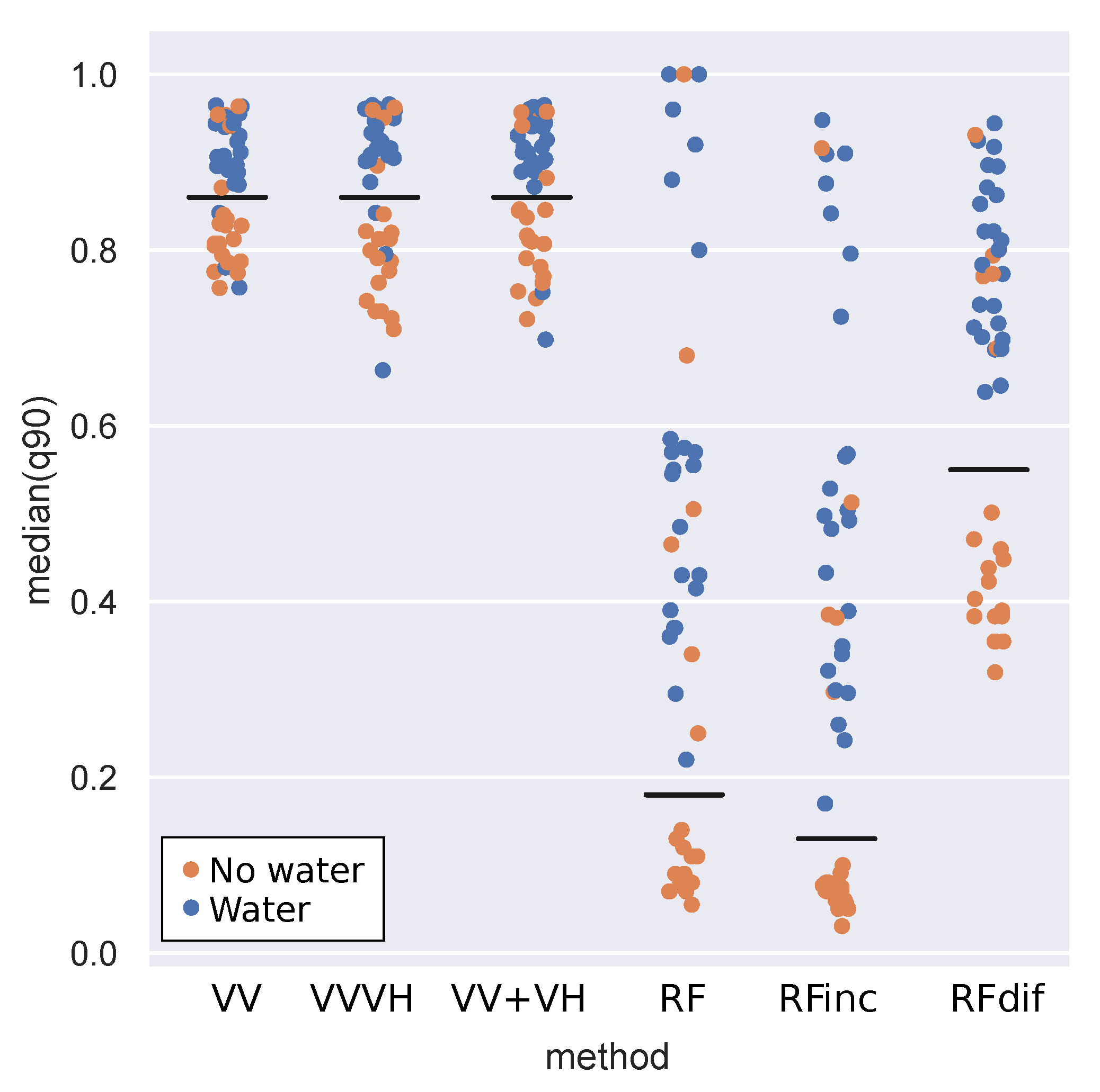
3.3. Differences
4. Discussion
5. Conclusions
Author Contributions
Funding
Data Availability Statement
Conflicts of Interest
Abbreviations
| RF | Random Forest |
| SAR | Synthetic Aperture Radar |
References
- Jongman, B.; Ward, P.; Aerts, J. Global exposure to river and coastal flooding: Long term trends and changes. Global Environ. Chang. 2012, 22, 823–835. [Google Scholar] [CrossRef]
- Hallegatte, S.; Green, C.; Nicholls, R.; Corfee-Morlot, J. Future flood losses in major coastal cities. Nat. Clim. Chang. 2013, 3, 802–806. [Google Scholar] [CrossRef]
- Muhadi, N.; Abdullah, A.; Bejo, S.; Mahadi, M.; Mijic, A. Image Segmentation Methods for Flood Monitoring System. Water 2020, 12, 1825. [Google Scholar] [CrossRef]
- Roy, R.; Gain, A.; Hurlbert, M.; Samat, N.; Tan, M.; Chan, N. Designing adaptation pathways for flood-affected households in Bangladesh. Environ. Dev. Sustain. 2020, 23, 5386–5410. [Google Scholar] [CrossRef]
- Pall, P.; Aina, T.; Stone, D.; Stott, P.; Nozawa, T.; Hilberts, A.; Lohmann, D.; Allen, M. Anthropogenic greenhouse gas contribution to flood risk in England and Wales in autumn 2000. Nature 2011, 470, 382–385. [Google Scholar] [CrossRef]
- Simonovic, S.; Kundzewicz, Z.; Wright, N. Floods and the COVID-19 pandemic—A new double hazard problem. WIREs Water 2021, 8, e1509. [Google Scholar] [CrossRef]
- Masson-Delmotte, V.; Zhai, P.; Pirani, A.; Connors, S.L.; Péan, C.; Berger, S.; Caud, N.; Chen, Y.; Goldfarb, L.; Gomis, M.I.; et al. Climate Change 2021: The Physical Science Basis. Contribution of Working Group I to the Sixth Assessment Report of the Intergovernmental Panel on Climate Change; Technical Summary; Cambridge University Press: Cambridge, UK, 2021. [Google Scholar] [CrossRef]
- CRED. A2023 Disasters in Numbers; Technical Report; Centre for Research on the Epidemiology of Disasters (CRED): Brussels, Belgium, 2023. [Google Scholar]
- Nabinejad, S.; Schüttrumpf, H. Flood risk management in arid and semi-arid areas: A comprehensive review of challenges, needs, and opportunities. Water 2023, 15, 3113. [Google Scholar] [CrossRef]
- Dokić, D.; Gavran, M.; Gregić, M.; Gantner, V. The impact of trade balance of agri-food products on the state’s ability to withstand the crisis. HighTech Innov. J. 2020, 1, 107–111. [Google Scholar] [CrossRef]
- Zhang, X.; Chan, N.; Pan, B.; Ge, X.; Yang, H. Mapping Flood by the Object-Based Method Using Backscattering Coefficient and Interference Coherence of Sentinel-1 Time Series. Sci. Total. Environ. 2021, 794, 148388. [Google Scholar] [CrossRef]
- Jongman, B.; Wagemaker, J.; Revilla-Romero, B.; De Perez, E. Early flood detection for rapid humanitarian response: Harnessing near real-time satellite and Twitter signals. ISPRS Int. J. Geo Inf. 2015, 4, 2246–2266. [Google Scholar] [CrossRef]
- Shen, X.; Anagnostou, E.; Allen, G.; Brakenridge, G.; Kettner, A. Near-real-time non-obstructed flood inundation mapping using synthetic aperture radar. Remote Sens. Environ. 2019, 221, 302–315. [Google Scholar] [CrossRef]
- McFeeters, S. The use of the Normalized Difference Water Index (NDWI) in the delineation of open water features. Int. J. Remote Sens. 1996, 17, 1425–1432. [Google Scholar] [CrossRef]
- Xu, H. Modification of normalised difference water index (NDWI) to enhance open water features in remotely sensed imagery. Int. J. Remote Sens. 2006, 27, 3025–3033. [Google Scholar] [CrossRef]
- Gu, Y.; Hunt, E.; Wardlow, B.; Basara, J.; Brown, J.; Verdin, J. Evaluation of MODIS NDVI and NDWI for vegetation drought monitoring using oklahoma mesonet soil moisture data. Geophys. Res. Lett. 2008, 35, 5. [Google Scholar] [CrossRef]
- Qiao, C.; Luo, J.; Sheng, Y.; Shen, Z.; Zhu, Z.; Ming, D. An adaptive water extraction method from remote sensing image based on NDWI. J. Indian Soc. Remote Sens. 2012, 40, 421–433. [Google Scholar] [CrossRef]
- Tao, S.; Fang, J.; Zhao, X.; Zhao, S.; Shen, H.; Hu, H.; Tang, Z.; Wang, Z.; Guo, Q. Rapid loss of lakes on the mongolian plateau. Proc. Natl. Acad. Sci. USA 2015, 112, 2281–2286. [Google Scholar] [CrossRef]
- Yan, P.; Zhang, Y.; Zhang, Y. A Study on Information Extraction of Water System in Semi-arid Regions with the Enhanced Water Index (EWI) and GIS Based Noise Remove Techniques. Remote Sens. Inf. 2007, 6, 62–67. [Google Scholar]
- Feyisa, G.; Meilby, H.; Fensholt, R.; Proud, S. Automated Water Extraction Index: A new technique for surface water mapping using Landsat imagery. Remote Sens. Environ. 2014, 140, 23–35. [Google Scholar] [CrossRef]
- Gstaiger, V.; Huth, J.; Gebhardt, S.; Kuenzer, C.; Wehrmann, T. Multi-sensoral and automated derivation of inundated areas using TerraSAR-X and ENVISAT ASAR data. Int. J. Remote Sens. 2012, 33, 7291–7304. [Google Scholar] [CrossRef]
- Lira, J. Segmentation and morphology of open water bodies from multispectral images. Int. J. Remote Sens. 2006, 27, 4015–4038. [Google Scholar] [CrossRef]
- Ko, B.; Kim, H.; Nam, J. Classification of potential water bodies using Landsat 8 OLI and a combination of two boosted random forest classifiers. Sensors 2015, 15, 13763–13777. [Google Scholar] [CrossRef] [PubMed]
- Sheng, Y.; Shah, C.; Smith, L. Automated image registration for hydrologic change detection in the lake-rich Arctic. IEEE Geosci. Remote Sensing Lett. 2008, 5, 414–418. [Google Scholar] [CrossRef]
- Jiang, Z.; Qi, J.; Su, S.; Zhang, Z.; Wu, J. Water body delineation using index composition and HIS transformation. Int. J. Remote Sens. 2012, 33, 3402–3421. [Google Scholar] [CrossRef]
- Sun, F.; Sun, W.; Chen, J.; Gong, P. Comparison and improvement of methods for identifying waterbodies in remotely sensed imagery. Int. J. Remote Sens. 2012, 33, 6854–6875. [Google Scholar] [CrossRef]
- Verpoorter, C.; Kutser, T.; Tranvik, L. Automated mapping of water bodies using Landsat multispectral data. Limnol. Oceanogr. Methods 2012, 10, 1037–1050. [Google Scholar] [CrossRef]
- Dong, Z.; Wang, G.; Amankwah, S.; Wei, X.; Hu, Y.; Feng, A. Monitoring the Summer Flooding in the Poyang Lake Area of China in 2020 Based on Sentinel-1 Data and Multiple Convolutional Neural Networks. Int. J. Appl. Earth Obs. Geoinf. 2021, 102, 102400. [Google Scholar] [CrossRef]
- Long, S.; Fatoyinbo, T.; Policelli, F. Flood extent mapping for namibia using change detection and thresholding with SAR. Environ. Res. Lett. 2014, 9, 035002. [Google Scholar] [CrossRef]
- Tian, H.; Wu, M.; Niu, Z.; Wang, C.; Zhao, X. Dryland crops recognition under complex planting structure based on radarsat-2 images. Trans. Chin. Soc. Agric. Eng. 2015, 31, 154–159. [Google Scholar]
- Li, S.; Tan, H.; Liu, Z.; Zhou, Z.; Liu, Y.; Zhang, W.; Liu, K.; Qin, B. Mapping High Mountain Lakes Using Space-Borne Near-Nadir SAR Observations. Remote Sens. 2018, 10, 1418. [Google Scholar] [CrossRef]
- Cui, J.; Zhang, X.; Wang, W.; Shen, Y. Integration of optical and SAR remote sensing images for crop-type mapping based on a novel object-oriented feature selection method. Int. J. Agric. Biol. Eng. 2020, 13, 178–190. [Google Scholar] [CrossRef]
- Liang, D.; Guo, H.; Zhang, L.; Li, H.; Wang, X. Sentinel-1 EW Mode Dataset for Antarctica from 2014–2020 Produced by the CASEarth Cloud Service Platform. Big Earth Data 2022, 6, 385–400. [Google Scholar] [CrossRef]
- Luo, X.; Hu, Z.; Liu, L. Investigating the seasonal dynamics of surface water over the Qinghai–Tibet Plateau using Sentinel-1 imagery and a novel gated multiscale ConvNet. Int. J. Digit. Earth 2023, 16, 1372–1394. [Google Scholar] [CrossRef]
- Torres, R.; Snoeij, P.; Geudtner, D.; Bibby, D.; Davidson, M.; Attema, E.; Potin, P.; Rommen, B.; Floury, N.; Brown, M. Gmes Sentinel-1 mission. Remote Sens. Environ. 2012, 120, 9–24. [Google Scholar] [CrossRef]
- Huth, J.; Gessner, U.; Klein, I.; Yesou, H.; Lai, X.; Oppelt, N.; Kuenzer, C. Analyzing water dynamics based on Sentinel-1 time series—a study at the Dongting Lake wetlands in China. Remote Sens. 2020, 12, 1761. [Google Scholar] [CrossRef]
- Singha, M.; Dong, J.; Sarmah, S.; You, N.; Zhou, Y.; Zhang, G.; Xiao, X. Identifying floods and flood-affected paddy rice fields in Bangladesh based on Sentinel-1 imagery and Google Earth Engine. ISPRS J. Photogramm. Remote Sens. 2020, 166, 278–293. [Google Scholar] [CrossRef]
- Gašparović, M.; Dobrinić, D. Comparative assessment of machine learning methods for urban vegetation mapping using multitemporal sentinel-1 imagery. Remote Sens. 2020, 12(12), 1952. [Google Scholar] [CrossRef]
- Li, Y.; Martinis, S.; Wieland, M. Urban Flood Mapping with an Active Self-Learning Convolutional Neural Network Based on TerraSAR-X Intensity and Interferometric Coherence. ISPRS J. Photogramm. Remote Sens. 2019, 152, 178–191. [Google Scholar] [CrossRef]
- Ordoyne, C.; Friedl, M. Using MODIS data to characterize seasonal inundation patterns in the Florida Everglades. Remote Sens. Environ. 2008, 112, 4107–4119. [Google Scholar] [CrossRef]
- Mahdianpari, M.; Salehi, B.; Mohammadimanesh, F.; Motagh, M. Random forest wetland classification using ALOS-2 L-band, RADARSAT-2 C-band, and TerraSAR-X imagery. ISPRS J. Photogramm. Remote Sens. 2017, 130, 13–31. [Google Scholar] [CrossRef]
- Mahdavi, S.; Salehi, B.; Granger, J.; Amani, M.; Brisco, B.; Huang, W. Remote sensing for wetland classification: A comprehensive review. GISci. Remote Sens. 2018, 55, 623–658. [Google Scholar] [CrossRef]
- Bao, Y.; Lin, L.; Wu, S.; Deng, K.; Petropoulos, G. Surface soil moisture retrievals over partially vegetated areas from the synergy of Sentinel-1 and Landsat 8 data using a modified water-cloud model. Int. J. Appl. Earth Obs. Geoinf. 2018, 72, 76–85. [Google Scholar] [CrossRef]
- Tian, H.; Li, W.; Wu, M.; Huang, N.; Li, G.; Li, X.; Niu, Z. Dynamic Monitoring of the Largest Freshwater Lake in China Using a New Water Index Derived from High Spatiotemporal Resolution Sentinel-1A Data. Remote Sens. 2017, 9, 521. [Google Scholar] [CrossRef]
- Oberstadler, R.; Hönsch, H.; Huth, D. Assessment of the mapping capabilities of ERS-1 SAR data for flood mapping: A case study in Germany. Hydrol. Process. 1997, 11, 1415–1425. [Google Scholar] [CrossRef]
- Bazi, Y.; Bruzzone, L.; Melgani, F. An unsupervised approach based on the generalized Gaussian model to automatic change detection in multitemporal SAR images. IEEE Trans. Geosci. Remote Sens. 2005, 43, 874–887. [Google Scholar] [CrossRef]
- Hostache, R. Estimation de niveaux d’eau en plaine inondée à partir d’images satellites radar et de données topographiques fines. Revue Télédétection (Remote Sens. J.) 2006, 6, 325–343. [Google Scholar]
- Pierdicca, N.; Chini, M.; Pulvirenti, L.; Macina, F. Integrating physical and topographic information into a fuzzy scheme to map flooded area by SAR. Sensors 2008, 8, 4151–4164. [Google Scholar] [CrossRef]
- Chini, M.; Piscini, A.; Cinti, F.; Amici, S.; Nappi, R.; DeMartini, P. The 2011 Tohoku (Japan) tsunami inundation and liquefaction investigated through optical, thermal, and SAR data. IEEE Geosci. Remote Sens. Lett. 2013, 10, 347–351. [Google Scholar] [CrossRef]
- Schumann, G.; Hostache, R.; Puech, C.; Hoffmann, L.; Matgen, P.; Pappenberger, F.; Pfister, L. High-resolution 3-D flood information from radar imagery for flood hazard management. IEEE Trans. Geosci. Remote Sens. 2007, 45, 1715–1725. [Google Scholar] [CrossRef]
- Chini, M.; Pelich, R.; Pulvirenti, L.; Pierdicca, N.; Hostache, R.; Matgen, P. Sentinel-1 InSAR coherence to detect floodwater in urban areas: Houston and Hurricane Harvey as a test case. Remote Sens. 2019, 11, 107. [Google Scholar] [CrossRef]
- Chini, M.; Hostache, R.; Giustarini, L.; Matgen, P. A hierarchical split-based approach for parametric thresholding of SAR images: Flood inundation as a test case. IEEE Trans. Geosci. Remote Sens. 2017, 55, 6975–6988. [Google Scholar] [CrossRef]
- Twele, A.; Cao, W.; Plank, S.; Martinis, S. Sentinel-1-based flood mapping: A fully automated processing chain. Int. J. Remote Sens. 2016, 37, 2990–3004. [Google Scholar] [CrossRef]
- De Roo, A.; Van Der Knijff, J.; Horritt, M.; Schmuck, G.; De Jong, S. Assessing flood damages of the 1997 Oder flood and the 1995 Meuse flood. In Proceedings of the Second International ITC Symposium on Operationalization of Remote Sensing, Enschede, The Netherlands; 1999; pp. 16–20. [Google Scholar]
- Townsend, P. Relationships between forest structure and the detection of flood inundation in forested wetlands using C-band SAR. Int. J. Remote Sens. 2002, 23, 443–460. [Google Scholar] [CrossRef]
- Pulvirenti, L.; Pierdicca, N.; Chini, M.; Guerriero, L. Monitoring flood evolution in vegetated areas using COSMO-SkyMed data: The Tuscany 2009 case study. IEEE J. Sel. Topics Appl. Earth Observ. Remote Sens. 2013, 6, 1807–1816. [Google Scholar] [CrossRef]
- Liang, J.; Liu, D. A local thresholding approach to flood water delineation using Sentinel-1 SAR imagery. ISPRS J. Photogramm. Remote Sens. 2020, 159, 53–62. [Google Scholar] [CrossRef]
- Otsu, N. A Threshold Selection Method from Gray-Level Histograms. IEEE Trans. Syst. Cybern. 1979, 9, 62–66. [Google Scholar] [CrossRef]
- Han, B.; Wu, Y. A novel active contour model driven by J-divergence entropy for SAR river image segmentation. Pattern Anal. Appl. 2018, 21, 613–627. [Google Scholar] [CrossRef]
- Huo, W.; Huang, Y.; Pei, J.; Zhang, Q.; Gu, Q.; Yang, J. Ship detection from ocean SAR image based on local contrast variance weighted information entropy. Sensors 2018, 18, 1196. [Google Scholar] [CrossRef]
- Huang, W.; DeVries, B.; Huang, C.; Lang, M.; Jones, J.; Creed, I.; Carroll, M. Automated Extraction of Surface Water Extent from Sentinel-1 Data. Remote Sens. 2018, 10, 797. [Google Scholar] [CrossRef]
- Insom, P.; Cao, C.; Boonsrimuang, P.; Liu, D.; Saokarn, A.; Yomwan, P.; Xu, Y. A Support Vector Mawchine-Based Particle Filter Method for Improved Flooding Classification. IEEE Geosci. Remote. Sens. Lett. 2015, 12, 1943–1947. [Google Scholar] [CrossRef]
- Skakun, S. A Neural Network Approach to Flood Mapping Using Satellite Imagery. Comput. Informatics 2010, 29, 1013–1024. [Google Scholar]
- Zeng, L.; Schmitt, M.; Li, L.; Zhu, X. Analysing Changes of the Poyang Lake Water Area Using Sentinel-1 Synthetic Aperture Radar Imagery. Int. J. Remote. Sens. 2017, 38, 7041–7069. [Google Scholar] [CrossRef]
- Mason, D.; Speck, R.; Devereux, B.; Schumann, G.; Neal, J.; Bates, P. Flood detection in urban areas using TerraSAR-X. IEEE Trans. Geosci. Remote Sens. 2010, 48, 882–894. [Google Scholar] [CrossRef]
- Mason, D.; Schumann, G.; Neal, J.; Garcia-Pintado, J.; Bates, P. Automatic near real-time selection of flood water levels from high resolution Synthetic Aperture Radar images for assimilation into hydraulic models: A case study. Remote Sens. Environ. 2012, 124, 705–716. [Google Scholar] [CrossRef]
- O’Grady, D.; Leblanc, M.; Gillieson, D. Use of ENVISAT ASAR Global Monitoring Mode to complement optical data in the mapping of rapid broad-scale flooding in Pakistan. Hydrol. Earth Syst. 2011, 15, 3475–3494. [Google Scholar] [CrossRef]
- Martinis, S.; Twele, A.; Voigt, S. Towards operational near real-time flood detection using a split-based automatic thresholding procedure on high resolution TerraSAR-X data. Nat. Hazard. Earth Syst. Sci. 2009, 9, 303–314. [Google Scholar] [CrossRef]
- Giustarini, L.; Hostache, R.; Kavetski, D.; Chini, M.; Corato, G.; Schlaffer, S.; Matgen, P. Probabilistic flood mapping using synthetic aperture radar data. IEEE Trans. Geosci. Remote Sens. 2016, 54, 6958–6969. [Google Scholar] [CrossRef]
- Pulvirenti, L.; Chini, M.; Pierdicca, N.; Guerriero, L.; Ferrazzoli, P. Flood monitoring using multi-temporal COSMO-SkyMed data: Image segmentation and signature interpretation. Remote Sens. Environ. 2011, 115, 990–1002. [Google Scholar] [CrossRef]
- Matgen, P.; Hostache, R.; Schumann, G.; Pfister, L.; Hoffmann, L.; Savenije, H. Towards an automated SAR-based flood monitoring system: Lessons learned from two case studies. Phys. Chem. Earth 2011, 36, 241–252. [Google Scholar] [CrossRef]
- Tong, X.; Luo, X.; Liu, S.; Xie, H.; Chao, W.; Liu, S.; Liu, S.; Makhinov, A.; Makhinova, A.; Jiang, Y. An Approach for Flood Monitoring by the Combined use of Landsat 8 Optical Imagery and COSMO-SkyMed Radar Imagery. ISPRS J. Photogramm. Remote Sens. 2018, 136, 144–153. [Google Scholar] [CrossRef]
- Cazals, C.; Rapinel, S.; Frison, P.; Bonis, A.; Mercier, G.; Mallet, C.; Corgne, S.; Rudant, J. Mapping and characterization of hydrological dynamics in a Coastal Marsh Using High Temporal Resolution Sentinel-1A Images. Remote Sens. 2016, 8, 570. [Google Scholar] [CrossRef]
- Bhardwaj, A.; Singh, M.; Joshi, P.; Snehmani; Singh, S.; Sam, L.; Gupta, R.; Kumar, R. A lake detection algorithm (LDA) using Landsat 8 data: A comparative approach in glacial environment. Int. J. Appl. Earth Obs. Geoinf. 2015, 38, 150–163. [Google Scholar] [CrossRef]
- Sheng, Y.; Song, C.; Wang, J.; Lyons, E.; Knox, B.; Cox, J.; Gao, F. Representative lake water extent mapping at continental scales using multi-temporal Landsat-8 imagery. Remote Sens. Environ. 2016, 185, 129–141. [Google Scholar] [CrossRef]
- Jiang, H.; Feng, M.; Zhu, Y.; Lu, N.; Huang, J.; Xiao, T. An automated method for extracting rivers and lakes from Landsat imagery. Remote Sens. 2014, 6, 5067–5089. [Google Scholar] [CrossRef]
- Yang, K.; Li, M.; Liu, Y.; Cheng, L.; Huang, Q.; Chen, Y. River detection in remotely sensed imagery using Gabor filtering and path opening. Remote Sens. 2015, 7, 8779–8802. [Google Scholar] [CrossRef]
- Li, W.; Gong, P. Continuous monitoring of coastline dynamics in western Florida with a 30-year time series of Landsat imagery. Remote Sens. Environ. 2016, 179, 196–209. [Google Scholar] [CrossRef]
- Wang, D.; Cui, X.; Xie, F.; Jiang, Z.; Shi, Z. Multi-feature sea–land segmentation based on pixel-wise learning for optical remote-sensing imagery. Int. J. Remote Sens. 2017, 38, 4327–4347. [Google Scholar] [CrossRef]
- Yang, X.; Qin, Q.; Grussenmeyer, P.; Koehl, M. Urban surface water body detection with suppressed built-up noise based on water indices from Sentinel-2 MSI imagery. Remote Sens. Environ. 2018, 219, 259–270. [Google Scholar] [CrossRef]
- Ngoc, D.; Loisel, H.; Jamet, C.; Vantrepotte, V.; Duforêt-Gaurier, L.; Minh, C.; Mangin, A. Coastal and inland water pixels extraction algorithm (WiPE) from spectral shape analysis and HSV transformation applied to Landsat 8 OLI and Sentinel-2 MSI. Remote Sens. Environ. 2019, 223, 208–228. [Google Scholar] [CrossRef]
- Cai, Y.; Li, X.; Zhang, M.; Lin, H. Mapping wetland using the object-based stacked generalization method based on multi-temporal optical and SAR data. Int. J. Appl. Earth Obs. Geoinf. 2020, 92, 102164. [Google Scholar] [CrossRef]
- Hossain, M.; Chen, D. Segmentation for Object-Based Image Analysis (OBIA): A review of algorithms and challenges from remote sensing perspective. ISPRS J. Photogramm. Remote Sens. 2019, 150, 115–134. [Google Scholar] [CrossRef]
- Phiri, D.; Morgenroth, J.; Xu, C.; Hermosilla, T. Effects of pre-processing methods on Landsat OLI-8 land cover classification using OBIA and random forests classifier. Int. J. Appl. Earth Obs. Geoinf. 2018, 73, 170–178. [Google Scholar] [CrossRef]
- Isikdogan, F.; Bovik, A.; Passalacqua, P. Surface Water Mapping by Deep Learning. IEEE J. Sel. Top. Appl. Earth Obs. Remote Sens. 2017, 10, 4909–4918. [Google Scholar] [CrossRef]
- Isikdogan, L.; Bovik, A.; Passalacqua, P. Seeing through the clouds with deepwatermap. IEEE Geosci. Remote Sens. Lett. 2019, 17, 1662–1666. [Google Scholar] [CrossRef]
- Fang, W.; Wang, C.; Chen, X.; Wan, W.; Li, H.; Zhu, S.; Fang, Y.; Liu, B.; Hong, Y. Recognizing global reservoirs from landsat 8 images: A deep learning approach. RIEEE J. Sel. Top. Appl. Earth Obs. Remote Sens. 2019, 12, 3168–3177. [Google Scholar] [CrossRef]
- Luo, X.; Tong, X.; Hu, Z. An Applicable and Automatic Method for Earth Surface Water Mapping Based on Multispectral Images. Int. J. Appl. Earth Obs. Geoinf. 2021, 103, 102472. [Google Scholar] [CrossRef]
- Jiang, W.; He, G.; Long, T.; Ni, Y.; Liu, H.; Peng, Y.; Lv, K.; Wang, G. Multilayer Perceptron Neural Network for Surface Water Extraction in Landsat 8 OLI Satellite Images. Remote Sens. 2018, 10(5), 755. [Google Scholar] [CrossRef]
- Romero Díaz, A.; Belmonte Serrato, F.; Hernández Bastida, J. El Campo de Cartagena una visión global. Recorridos por el Campo de Cartagena. Control de la Degradación y uso Sostenible del Suelo; Instituto Mediterráneo del Agua: Murcia, Spain, 2011; pp. 17–48. [Google Scholar]
- CARM. Estadística Agraria de Murcia. 2022–2023. Technical Report, Comunidad Autónoma de la Región de Murcia. 2023. Available online: https://esam.carm.es/wp-content/uploads/2024/10/ESTADISTICA-AGRARIA-DE-MURCIA2022-2023-rev1.pdf (accessed on 29 January 2024).
- Martínez, J.; Esteve, M.; Martínez-Paz, J.; Carreño, F.; Robledano, F.; Ruiz, M.; Alonso, F. Simulating management options and scenarios to control nutrient load to Mar Menor, Southeast Spain. Transitional Waters Monogr. TWM Transit. Waters Monogr 2007, 1. [Google Scholar] [CrossRef]
- Giménez-Casalduero, F.; Gomariz-Castillo, F.; Alonso-Sarría, F.; Cortés, E.; Izquierdo-Muñoz, A.; Ramos-Esplá, A. Pinna nobilis in the Mar Menor coastal lagoon: A story of colonization and uncertainty. Mar. Ecol. Prog. Ser. 2020, 652, 77–94. [Google Scholar] [CrossRef]
- Pérez Morales, A.; Romero Díaz, A.; Caballero Pedraza, A. The Urbanisation Process and its Influence on the Increase in Flooding (Region of Murcia, Campo de Cartagena-Mar Menor, South-east Spain). In Crisis, Globalizations and Social and Regional Imbalances in Spain; Asociación de Geógrafos Españolas (AGE): Madrid, Spain, 2016; pp. 92–103. [Google Scholar]
- Pérez-Morales, A.; Gil-Guirado, S.; Olcina-Cantos, J. Housing bubbles and the increase of flood exposure. Failures in flood risk management on the Spanish south-eastern coast (1975–2013). J. Flood Risk Manag. 2015, 2015, S302–S313. [Google Scholar] [CrossRef]
- MITECO. Informe de Seguimiento del Plan de Gestión del Riesto de Inundación de la Demarcación Hidrográfica del Segura; Technical Report; Ministerio para la Transición Ecológica y el Reto Demográfico. Gobierno de España.: Madrid, Spain, 2019. [Google Scholar]
- Cortés-Melendreras, E.; Gomariz-Castillo, F.; Alonso-Sarría, F.; Martín, F.J.G.; Murcia, J.; Canales-Cáceres, R.; Esplá, A.A.R.; Barberáe, C.; Giménez-Casalduero, F. The relict population of Pinna nobilis in the Mar Menor is facing an uncertain future. Mar. Pollut. Bull. 2022, 185, 114376. [Google Scholar] [CrossRef]
- European Space Agency. Sentinel-2 Data; Technical Report; European Space Agency: Paris, France, 2023. [Google Scholar]
- Lang, M.W.; Townsend, P.A.; Kasischke, E.S. Influence of incidence angle on detecting flooded forests using C-HH synthetic aperture radar data. Remote Sens. Environ. 2008, 112, 3898–3907. [Google Scholar] [CrossRef]
- Filipponi, F. Sentinel-1 GRD preprocessing workflow. Proceedings 2019, 18, 11. [Google Scholar] [CrossRef]
- Breiman, L. Random Forests. Mach. Learn. 2001, 45, 5–32. [Google Scholar] [CrossRef]
- Masís, S. Interpretable Machine Learning with Python; Packt Publishing: Birmingham, UK, 2021; p. 715. [Google Scholar]
- Chen, Y.; Qiao, S.; Zhang, G.; Xu, Y.; Chen, L. Wu, L. Investigating the potential use of Sentinel-1 data for monitoring wetland water level changes in China’s Momoge National Nature Reserve. PeerJ 2020, 8, 20. [Google Scholar]

| Event | Images S1A | Images S1B |
|---|---|---|
| 1 | S1A_IW_GRDH_1SDV_20161124T061008_20161124T061033_014080_016B63_DABC | S1B_IW_GRDH_1SDV_20161224T060925_20161224T060950_003534_0060AE_C881 |
| S1A_IW_GRDH_1SDV_20161124T061008_20161124T061033_014080_016B63_DABC | ||
| S1A_IW_GRDH_1SDV_20161206T061007_20161206T061032_014255_0170E4_37C1 | ||
| S1A_IW_GRDH_1SDV_20161206T061032_20161206T061057_014255_0170E4_B0B3 | ||
| S1A_IW_GRDH_1SDV_20161218T061007_20161218T061032_014430_017666_2AF7 | ||
| S1A_IW_GRDH_1SDV_20161218T061032_20161218T061057_014430_017666_CA83 | ||
| 2 | S1A_IW_GRDH_1SDV_20170111T061005_20170111T061030_014780_01811D_9DA1 | S1B_IW_GRDH_1SDV_20170117T060923_20170117T060948_003884_006B01_CCA8 |
| S1A_IW_GRDH_1SDV_20170111T061030_20170111T061055_014780_01811D_E66E | ||
| S1A_IW_GRDH_1SDV_20170123T061005_20170123T061030_014955_018698_AE68 | ||
| S1A_IW_GRDH_1SDV_20170123T061030_20170123T061055_014955_018698_1FBC | ||
| 3 | S1A_IW_GRDH_1SDV_20170827T061008_20170827T061033_018105_01E680_CC5A | S1B_IW_GRDH_1SDV_20170821T060945_20170821T061010_007034_00C646_C9A9 |
| S1A_IW_GRDH_1SDV_20170827T061033_20170827T061058_018105_01E680_8DAE | S1B_IW_GRDH_1SDV_20170902T060945_20170902T061010_007209_00CB57_12A7 | |
| 4 | S1A_IW_GRDH_1SDV_20180118T061007_20180118T061032_020205_022790_28AD | S1B_IW_GRDH_1SDV_20180124T060944_20180124T061009_009309_010B3B_A34D |
| S1A_IW_GRDH_1SDV_20180118T061032_20180118T061057_020205_022790_0687 | ||
| S1A_IW_GRDH_1SDV_20180130T061006_20180130T061031_020380_022D20_124A | ||
| S1A_IW_GRDH_1SDV_20180130T061031_20180130T061056_020380_022D20_C24E | ||
| 5 | S1A_IW_GRDH_1SDV_20180506T061008_20180506T061033_021780_025963_F8C4 | S1B_IW_GRDH_1SDV_20180430T060945_20180430T061010_010709_0138F2_C906 |
| S1A_IW_GRDH_1SDV_20180506T061033_20180506T061058_021780_025963_AB5D | S1B_IW_GRDH_1SDV_20180512T060946_20180512T061011_010884_013E97_6108 | |
| 6 | S1A_IW_GRDH_1SDV_20180518T061009_20180518T061034_021955_025EF3_CB2A | S1B_IW_GRDH_1SDV_20180524T060946_20180524T061011_011059_014449_A2C7 |
| S1A_IW_GRDH_1SDV_20180518T061034_20180518T061059_021955_025EF3_85A8 | S1B_IW_GRDH_1SDV_20180605T060947_20180605T061012_011234_0149EC_FF2D | |
| S1A_IW_GRDH_1SDV_20180530T061009_20180530T061034_022130_026493_4F1B | ||
| S1A_IW_GRDH_1SDV_20180530T061034_20180530T061059_022130_026493_C1EE | ||
| 7 | S1A_IW_GRDH_1SDV_20180903T061015_20180903T061040_023530_028FEB_799C | S1B_IW_GRDH_1SDV_20180828T060952_20180828T061017_012459_016F9A_6935 |
| S1A_IW_GRDH_1SDV_20180903T061040_20180903T061105_023530_028FEB_ECF4 | S1B_IW_GRDH_1SDV_20180909T060953_20180909T061018_012634_017500_5662 | |
| S1A_IW_GRDH_1SDV_20180915T061015_20180915T061040_023705_029586_A4EA | S1B_IW_GRDH_1SDV_20180921T060953_20180921T061018_012809_017A59_B633 | |
| S1A_IW_GRDH_1SDV_20180915T061040_20180915T061105_023705_029586_0057 | ||
| 7 | S1A_IW_GRDH_1SDV_20181114T061016_20181114T061041_024580_02B2D5_5589 | S1B_IW_GRDH_1SDV_20181003T060953_20181003T061018_012984_017FB6_0281 |
| S1A_IW_GRDH_1SDV_20181114T061041_20181114T061106_024580_02B2D5_EE00 | S1B_IW_GRDH_1SDV_20181108T060953_20181108T061018_013509_018FF3_AD05 | |
| S1B_IW_GRDH_1SDV_20181120T060953_20181120T061018_013684_019579_7E62 | ||
| 9 | S1A_IW_GRDH_1SDV_20190407T061013_20190407T061038_026680_02FE88_359D | S1B_IW_GRDH_1SDV_20190413T060951_20190413T061016_015784_01DA0A_1C2E |
| S1A_IW_GRDH_1SDV_20190407T061038_20190407T061103_026680_02FE88_34E6 | S1B_IW_GRDH_1SDV_20190425T060951_20190425T061016_015959_01DFD4_B029 | |
| S1A_IW_GRDH_1SDV_20190419T061013_20190419T061038_026855_0304E2_5040 | ||
| S1A_IW_GRDH_1SDV_20190419T061038_20190419T061103_026855_0304E2_9FB5 | ||
| 10 | S1A_IW_GRDH_1SDV_20190910T061021_20190910T061046_028955_034891_EDAB | S1B_IW_GRDH_1SDV_20190904T060959_20190904T061024_017884_021A81_9492 |
| S1A_IW_GRDH_1SDV_20190910T061046_20190910T061111_028955_034891_D799 | ||
| S1A_IW_GRDH_1SDV_20190916T180159_20190916T180224_029050_034BE2_3693 | ||
| S1A_IW_GRDH_1SDV_20190916T180224_20190916T180249_029050_034BE2_F390 | ||
| 11 | S1A_IW_GRDH_1SDV_20191121T061022_20191121T061047_030005_036CD8_C962 | S1B_IW_GRDH_1SDV_20191127T060959_20191127T061024_019109_024106_5C20 |
| S1A_IW_GRDH_1SDV_20191121T061047_20191121T061112_030005_036CD8_D8B5 | S1B_IW_GRDH_1SDV_20191209T060959_20191209T061024_019284_02468F_3DE6 | |
| S1A_IW_GRDH_1SDV_20191203T061021_20191203T061046_030180_0372EA_EB2D | ||
| S1A_IW_GRDH_1SDV_20191203T061046_20191203T061111_030180_0372EA_EA7B | ||
| 12 | S1A_IW_GRDH_1SDV_20200114T180209_20200114T180234_030800_03886B_6543 | S1B_IW_GRDH_1SDV_20191221T060958_20191221T061023_019459_024C21_7934 |
| S1A_IW_GRDH_1SDV_20200126T180208_20200126T180233_030975_038E95_75DB | S1B_IW_GRDH_1SDV_20200120T180118_20200120T180143_019904_025A67_3AEA | |
| S1B_IW_GRDH_1SDV_20200120T180143_20200120T180208_019904_025A67_0A0D | ||
| 13 | S1A_IW_GRDH_1SDV_20200314T180208_20200314T180233_031675_03A6D3_461A | S1B_IW_GRDH_1SDV_20200320T180118_20200320T180143_020779_02766F_D3C8 |
| S1A_IW_GRDH_1SDV_20200326T180208_20200326T180233_031850_03ACFC_08DF | S1B_IW_GRDH_1SDV_20200320T180143_20200320T180208_020779_02766F_7126 | |
| S1A_IW_GRDH_1SDV_20200407T180208_20200407T180233_032025_03B327_FE7E | S1B_IW_GRDH_1SDV_20200401T180118_20200401T180143_020954_027BF7_C274 | |
| S1B_IW_GRDH_1SDV_20200401T180143_20200401T180208_020954_027BF7_AF41 | ||
| 14 | S1A_IW_GRDH_1SDV_20201227T180216_20201227T180241_035875_043370_8BB4 | S1B_IW_GRDH_1SDV_20210102T180125_20210102T180150_024979_02F915_487F |
| S1A_IW_GRDH_1SDV_20210108T180215_20210108T180240_036050_043984_D6D1 | S1B_IW_GRDH_1SDV_20210102T180150_20210102T180215_024979_02F915_E8E3 | |
| S1B_IW_GRDH_1SDV_20210114T180125_20210114T180150_025154_02FEB3_C368 | ||
| S1B_IW_GRDH_1SDV_20210114T180150_20210114T180215_025154_02FEB3_1C3D | ||
| 15 | S1A_IW_GRDH_1SDV_20210225T180214_20210225T180239_036750_0451E1_B229 | S1B_IW_GRDH_1SDV_20210303T180123_20210303T180148_025854_031561_9DD0 |
| S1A_IW_GRDH_1SDV_20210309T180214_20210309T180239_036925_0457FF_DAB6 | S1B_IW_GRDH_1SDV_20210303T180148_20210303T180213_025854_031561_413C | |
| S1B_IW_GRDH_1SDV_20210315T180123_20210315T180148_026029_031B0C_8AF2 | ||
| S1B_IW_GRDH_1SDV_20210315T180148_20210315T180213_026029_031B0C_B917 | ||
| 16 | S1A_IW_GRDH_1SDV_20210402T180214_20210402T180239_037275_046426_6E19 | S1B_IW_GRDH_1SDV_20210327T180124_20210327T180149_026204_03209B_E1CC |
| S1A_IW_GRDH_1SDV_20210414T180214_20210414T180239_037450_046A34_6D58 | S1B_IW_GRDH_1SDV_20210327T180149_20210327T180214_026204_03209B_4CE6 | |
| S1A_IW_GRDH_1SDV_20210426T180215_20210426T180240_037625_04703C_0C1D | S1B_IW_GRDH_1SDV_20210408T180124_20210408T180149_026379_032624_B065 | |
| S1B_IW_GRDH_1SDV_20210408T180149_20210408T180214_026379_032624_4D64 | ||
| S1B_IW_GRDH_1SDV_20210420T180125_20210420T180150_026554_032BC7_B070 | ||
| S1B_IW_GRDH_1SDV_20210420T180150_20210420T180215_026554_032BC7_42BB | ||
| S1B_IW_GRDH_1SDV_20210502T180125_20210502T180150_026729_033160_AEC5 | ||
| S1B_IW_GRDH_1SDV_20210502T180150_20210502T180215_026729_033160_3792 | ||
| 17 | S1A_IW_GRDH_1SDV_20210520T180216_20210520T180241_037975_047B69_58A3 | S1B_IW_GRDH_1SDV_20210514T180126_20210514T180151_026904_0336D6_D9F3 |
| S1B_IW_GRDH_1SDV_20210514T180151_20210514T180216_026904_0336D6_80F5 | ||
| S1B_IW_GRDH_1SDV_20210526T180126_20210526T180151_027079_033C2F_3EDB | ||
| S1B_IW_GRDH_1SDV_20210526T180151_20210526T180216_027079_033C2F_19C8 | ||
| 18 | S1A_IW_GRDH_1SDV_20220214T061030_20220214T061055_041905_04FD4E_6B2E | |
| S1A_IW_GRDH_1SDV_20220214T061055_20220214T061120_041905_04FD4E_F6EB | ||
| S1A_IW_GRDH_1SDV_20220220T180219_20220220T180244_042000_0500A2_3CF0 | ||
| S1A_IW_GRDH_1SDV_20220226T061030_20220226T061055_042080_050355_6088 | ||
| S1A_IW_GRDH_1SDV_20220226T061055_20220226T061120_042080_050355_B606 | ||
| S1A_IW_GRDH_1SDV_20220304T180219_20220304T180244_042175_050694_B224 | ||
| S1A_IW_GRDH_1SDV_20220310T061030_20220310T061055_042255_050941_03BA | ||
| S1A_IW_GRDH_1SDV_20220310T061055_20220310T061120_042255_050941_8676 | ||
| S1A_IW_GRDH_1SDV_20220316T180219_20220316T180244_042350_050C8C_F393 | ||
| S1A_IW_GRDH_1SDV_20220322T061031_20220322T061056_042430_050F38_EA76 | ||
| S1A_IW_GRDH_1SDV_20220322T061056_20220322T061121_042430_050F38_2BDD | ||
| S1A_IW_GRDH_1SDV_20220328T180220_20220328T180245_042525_05127F_A171 | ||
| S1A_IW_GRDH_1SDV_20220403T061031_20220403T061056_042605_051528_75D1 | ||
| S1A_IW_GRDH_1SDV_20220403T061056_20220403T061121_042605_051528_1418 | ||
| 19 | S1A_IW_GRDH_1SDV_20220924T180229_20220924T180254_045150_056567_4E1C | |
| S1A_IW_GRDH_1SDV_20220930T061040_20220930T061105_045230_056802_42A6 | ||
| S1A_IW_GRDH_1SDV_20220930T061105_20220930T061130_045230_056802_6199 | ||
| S1A_IW_GRDH_1SDV_20221006T180229_20221006T180254_045325_056B40_4506 | ||
| S1A_IW_GRDH_1SDV_20221012T061040_20221012T061105_045405_056DEA_C6B7 | ||
| S1A_IW_GRDH_1SDV_20221012T061105_20221012T061130_045405_056DEA_9C11 |
| Event | Initial Date | Final Date | Mean Rainfall | Max Rainfall | Duration |
|---|---|---|---|---|---|
| 1 | 04/12/2016:09 | 20/12/2016:00 | 210.6 | 316.0 | 15.62 |
| 2 | 19/01/2017:08 | 19/01/2017:21 | 58.4 | 84.2 | 0.54 |
| 3 | 29/08/2017:10 | 30/08/2017:14 | 30.4 | 44.2 | 1.17 |
| 4 | 27/01/2018:22 | 28/01/2018:16 | 30.3 | 46.27 | 0.75 |
| 5 | 09/05/2018:11 | 10/05/2018:21 | 7.7 | 35.75 | 1.42 |
| 6 | 29/05/2018:09 | 03/06/2018:03 | 12.1 | 32.8 | 4.75 |
| 7 | 08/09/2018:05 | 15/09/2018:16 | 35.6 | 61.2 | 6.46 |
| 8 | 14/11/2018:19 | 19/11/2018:12 | 92.7 | 135.6 | 4.71 |
| 9 | 19/04/2019:00 | 22/04/2019:21 | 101.7 | 132.4 | 3.87 |
| 10 | 10/09/2019:15 | 12/09/2019:20 | 195.2 | 283.7 | 2.21 |
| 11 | 01/12/2019:22 | 04/12/2019:08 | 65.6 | 157.5 | 2.41 |
| 12 | 19/01/2020:00 | 22/01/2020:11 | 81.4 | 110.3 | 3.46 |
| 13 | 21/03/2020:00 | 04/04/2020:23 | 144.9 | 186.8 | 14.96 |
| 14 | 04/01/2021:00 | 12/01/2021:23 | 43.7 | 72.3 | 8.96 |
| 15 | 05/03/2021:00 | 12/03/2021:23 | 54.7 | 80.6 | 7.96 |
| 16 | 06/04/2021:00 | 28/04/2021:23 | 51.9 | 85.6 | 22.96 |
| 17 | 22/05/2021:00 | 25/05/2021:23 | 57.6 | 79.2 | 3.96 |
| 18 | 23/02/2022:00 | 28/03/2022:23 | 165 | 231.9 | 5.96 |
| 19 | 04/10/2022:00 | 11/10/2022:23 | 32.4 | 118.8 | 7.96 |
| Predictor | Mean Error | Std Error | Mean Threshold | Std Threshold | Mean Accuracy |
|---|---|---|---|---|---|
| VV | 0.169 | 0.083 | −14.098 | 1.085 | 0.831 |
| VH | 0.263 | 0.109 | −20.451 | 0.963 | 0.737 |
| VVHV | 0.140 | 0.081 | 444.224 | 42.669 | 0.86 |
| VV/VH | 0.443 | 0.109 | 0.788 | 0.061 | 0.557 |
| VV+VH | 0.142 | 0.080 | −34.838 | 2.226 | 0.858 |
| VV-VH | 0.667 | 0.124 | 6.664 | 0.882 | 0.333 |
| VV | VVVH | VV+VH | RFprob | RFinc | RFdif | |||||||
|---|---|---|---|---|---|---|---|---|---|---|---|---|
| N | W | N | W | N | W | N | W | N | W | N | W | |
| N | 15 | 5 | 15 | 5 | 15 | 5 | 14 | 6 | 15 | 5 | 15 | 5 |
| W | 3 | 21 | 3 | 21 | 2 | 22 | 1 | 23 | 0 | 24 | 0 | 24 |
| accuracy | 0.818 | 0.818 | 0.841 | 0.841 | 0.886 | 0.886 | ||||||
| kappa | 0.63 | 0.63 | 0.675 | 0.672 | 0.766 | 0.766 | ||||||
| Metric | Accuracy 0.5 | AUC | Threshold | Accuracy Th |
|---|---|---|---|---|
| VV | 0.569 | 0.56 | 0.86 | 0.6207 |
| VVVH | 0.599 | 0.59 | 0.834 | 0.632 |
| VV+VH | 0.596 | 0.594 | 0.815 | 0.633 |
| RFprob | 0.599 | 0.665 | 0.04 | 0.651 |
| RFinc | 0.597 | 0.598 | 0.091 | 0.642 |
| RFdif | 0.617 | 0.513 | 0.436 | 0.645 |
| RFprob | RFFA | RFinc | RFIncFA | RFDif | |
|---|---|---|---|---|---|
| Precipitation | −0.005 | 0.322 | 0.141 | 0.516 | −0.053 |
| Max. precipit. | 0.067 | 0.371 | 0.234 | 0.572 | −0.091 |
Disclaimer/Publisher’s Note: The statements, opinions and data contained in all publications are solely those of the individual author(s) and contributor(s) and not of MDPI and/or the editor(s). MDPI and/or the editor(s) disclaim responsibility for any injury to people or property resulting from any ideas, methods, instructions or products referred to in the content. |
© 2025 by the authors. Licensee MDPI, Basel, Switzerland. This article is an open access article distributed under the terms and conditions of the Creative Commons Attribution (CC BY) license (https://creativecommons.org/licenses/by/4.0/).
Share and Cite
Alonso-Sarria, F.; Valdivieso-Ros, C.; Molina-Pérez, G. Detecting Flooded Areas Using Sentinel-1 SAR Imagery. Remote Sens. 2025, 17, 1368. https://doi.org/10.3390/rs17081368
Alonso-Sarria F, Valdivieso-Ros C, Molina-Pérez G. Detecting Flooded Areas Using Sentinel-1 SAR Imagery. Remote Sensing. 2025; 17(8):1368. https://doi.org/10.3390/rs17081368
Chicago/Turabian StyleAlonso-Sarria, Francisco, Carmen Valdivieso-Ros, and Gabriel Molina-Pérez. 2025. "Detecting Flooded Areas Using Sentinel-1 SAR Imagery" Remote Sensing 17, no. 8: 1368. https://doi.org/10.3390/rs17081368
APA StyleAlonso-Sarria, F., Valdivieso-Ros, C., & Molina-Pérez, G. (2025). Detecting Flooded Areas Using Sentinel-1 SAR Imagery. Remote Sensing, 17(8), 1368. https://doi.org/10.3390/rs17081368