Article

AGCD: An Attention-Guided Graph Convolution Network for Change Detection of Remote Sensing Images

1
College of Computer Science and Software Engineering, Hohai University, Nanjing 211100, China
2
Key Laboratory of Water Big Data Technology of Ministry of Water Resources, Hohai University, Nanjing 211100, China
*
Author to whom correspondence should be addressed.
Remote Sens. 2025, 17(8), 1367; https://doi.org/10.3390/rs17081367
Submission received: 25 January 2025 / Revised: 2 April 2025 / Accepted: 8 April 2025 / Published: 11 April 2025

Abstract

:
Change detection is a crucial field in remote sensing image analysis for tracking environmental dynamics. Although convolutional neural networks (CNNs) have made impressive strides in this field, their grid-based processing structures struggle to capture abundant semantics and complex spatial-temporal correlations of bitemporal features, leading to high uncertainty in distinguishing true changes from pseudo changes. To overcome these limitations, we propose the Attention-guided Graph convolution network for Change Detection (AGCD), a novel framework that integrates a graph convolutional network (GCN) and an attention mechanism to enhance change-detection performance. AGCD introduces three novel modules, including Graph-level Feature Difference Module (GFDM) for enhanced feature interaction, Multi-scale Feature Fusion Module (MFFM) for detailed semantic representation and Spatial-Temporal Attention Module (STAM) for refined spatial-temporal dependency modeling. These modules enable AGCD to reduce pseudo changes triggered by seasonal variations and varying imaging conditions, thereby improving the accuracy and reliability of change-detection results. Extensive experiments on three benchmark datasets demonstrate that AGCD’s superior performance, achieving the best F1-score of 90.34% and IoU of 82.38% on the LEVIR-CD dataset and outperforming existing state-of-the-art methods by a notable margin.

1. Introduction

Change detection is of significance in the field of remote sensing images, offering critical insights into the temporal dynamics of our environments [1]. These changes may encompass the constructions of new infrastructures, the demolitions of existing structures and the shifts in land-use forms. The importance of change detection lies in its wide range of applications, such as urban planning, environmental monitoring, disaster management and infrastructure development [2]. Advances in satellite technology has remarkably improved the availability and quality of satellite images, which enables more accurate monitoring of land cover types and more comprehensive analysis of land cover changes [3,4,5,6,
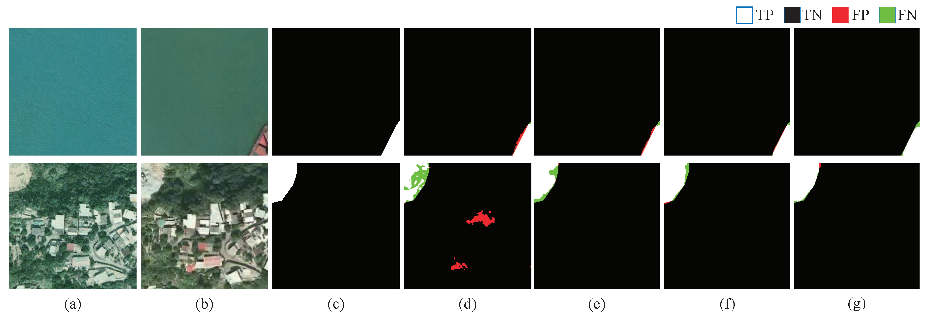
7]. However, as shown in 
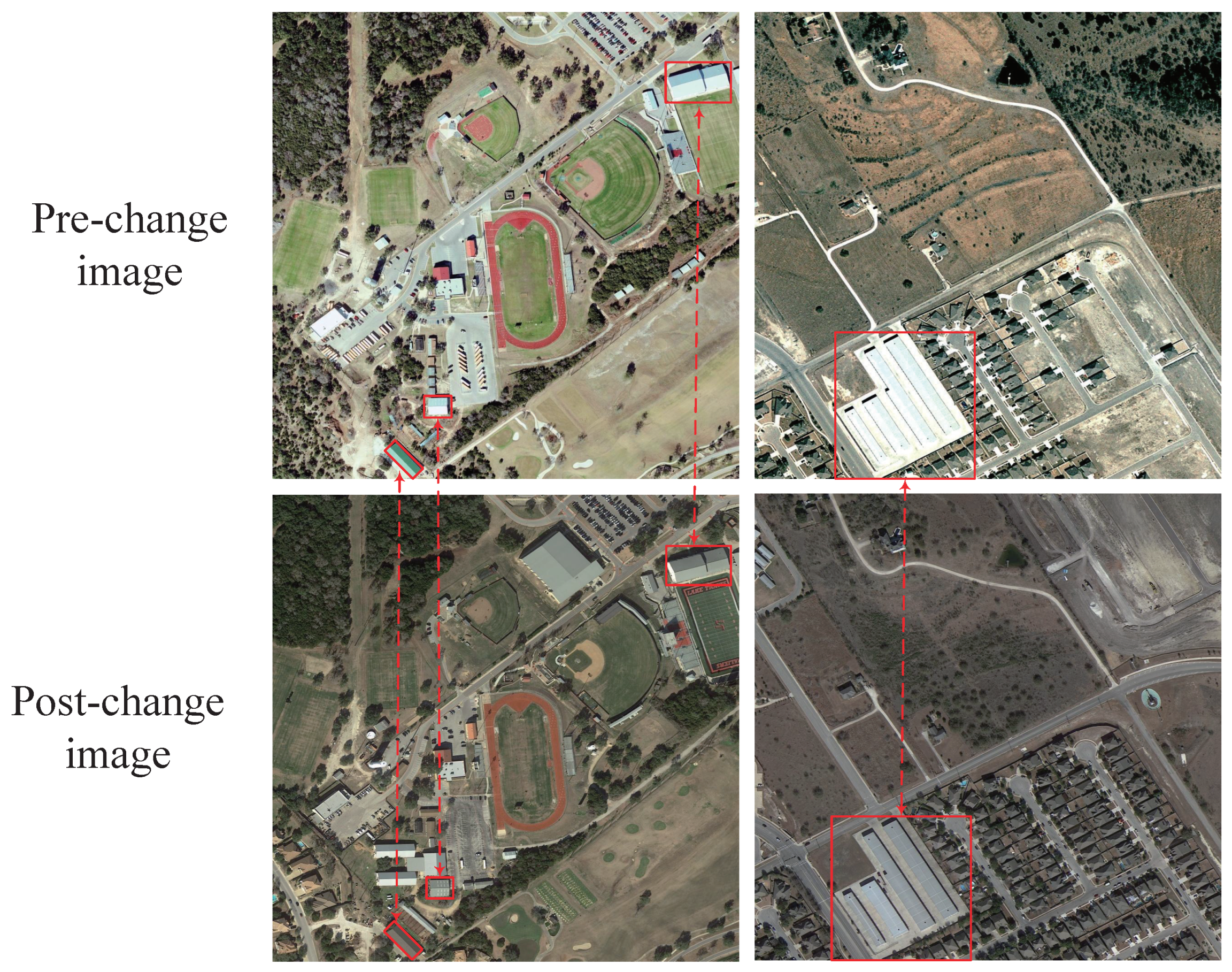
Figure 1, change detection in remote sensing images remains challenging due to the presence of pseudo changes caused by seasonal variations, varying imaging conditions and sensor noise. In light of this, mitigating pseudo change influence and thereby improving change-detection accuracy remain critical research objectives.
Traditional methods for change detection in remote sensing images such as pixel-based [8,9,10,11] and object-based approaches [12,13,14,15] have been widely studied. Pixel-based methods analyze changes between bitemporal images on a pixel-by-pixel basis, while object-based methods group pixels into homogeneous objects and analyze changes at the object level. However, both approaches are sensitive to noise and threshold selection, and their robustness to pseudo changes caused by illumination variations and seasonal changes is also limited, leading to poor change-detection performance.
Recently, with the development of deep learning (DL) techniques, DL-based methods have emerged as powerful alternatives to effectively improve change-detection performance. DL-based methods, represented by CNN-based and Transformer-based methods, leverage neural networks to effectively mine rich semantic features [16,17,18,19], enabling precise identification of changes over time in remote sensing images. For example, Daudt et al. [20] proposed fully convolution siamese networks, marking the first integration of siamese networks with fully convolutional architectures for change detection. However, this method struggles to effectively capture deep semantic information within images, resulting in suboptimal detection performance. Since then, many efforts have been dedicated to improving the ability to reduce pseudo changes and enhancing change-detection accuracy. Specifically, Zhang et al. [21] proposed feature difference CNN, which utilized a carefully designed loss function to learn the magnitude of changes. The learned change magnitude serves as prior knowledge to mitigate the impacts of pseudo changes. Shi et al. [22] proposed a deeply supervised network for change detection. By incorporating a metric module and a convolutional block attention module (CBAM), this approach effectively reduced the influence of pseudo changes and enhanced change-detection performance. However, the limited size of the receptive field in CNN structures poses challenges in capturing long-range dependencies across both space and time [23,24], thus hindering their further advancements in change detection. To address these limitations, Transformers, introduced in 2017 [25], have emerged as promising solutions. Unlike CNNs, Transformers excel at capturing global features and modeling long-range dependencies [26,27], which has contributed to their growing prominence in remote sensing image change detection. For instance, Chen et al. [28] introduced a lightweight Transformer-based model known as BIT for change detection; BIT identified change areas by extracting a concise token set that captures high-level features, demonstrating enhanced efficiency and accuracy over purely convolutional methods. Zhao et al. [29] introduced a hybrid network combining CNNs with a Transformer decoder. This approach employed multi-stage siamese CNNs to extract bitemporal features, which were then transformed into semantic tokens by the Transformer decoder to enhance feature interaction, demonstrating notable robustness against pseudo changes. Similarly, to mitigate the interference of pseudo changes, Xu et al. [30] proposed a Transformer-based network that encapsulated bitemporal features into semantic tokens for effective information exchange and incorporated graph reasoning to refine the contours of change areas.
Although Transformer architectures have demonstrated strong performance in change detection tasks, their efficiency is often hindered by high computational demands and quadratic complexity. To address these limitations, Mamba was introduced, leveraging a selective state-space model [31]. Since then, researchers have actively explored the incorporation of Mamba into change detection. For instance, Zhao et al. [32] proposed RSMamba, an innovative framework that introduced an omnidirectional scanning technique to capture contextual information across eight directions in remote sensing images. Benefiting from the linear complexity of the space state model, this method eliminated the need for cropping of large-scale remote sensing images, reducing semantic loss while maintaining high precision and computational efficiency. Chen et al. [33] introduced ChangeMamba, which integrated sequential, cross and parallel modeling mechanisms into a visual Mamba architecture, effectively modeling spatial-temporal relationships between bitemporal images and facilitating precise change detection. Beyond the computational challenges, Transformers also inherently face challenges due to their intrinsic sequence-based structure. While this structure allows Transformers to effectively model dependencies in sequential data, it also presents limitations when dealing with non-Euclidean data, making them less flexible for capturing complex, non-sequential relationships in remote sensing images, where interactions between different objects and landforms cannot be easily modeled as sequences. Recently, GCNs have gained traction across a wide range of domains, starting with their first proposal in [34] for semi-supervised classification, and expanding to graph-representation learning [35], social network analysis [36] and bioinformatics [37]. Compared to CNNs and Transformers, GCNs excel in feature learning on non-Euclidean data by aggregating node features based on their adjacency within the graph structure, offering a flexible and powerful approach for feature extraction and interaction in remote sensing change-detection tasks. For example, Song et al. [38] proposed GCN-based siamese network, which integrated a hybrid backbone combining over-parameterized CNN and vision graph neural network (ViG) to reduce the number of parameters while maintaining high change-detection performance. Yu et al. [39] proposed a multi-scale graph reasoning network for change detection. This method projected image features to graph vertices and utilized GCN for information propagation across vertices, improving feature fusion and interaction. Jiang et al [40] proposed a hybrid method that combined GCN and Transformer. The method utilized GCN to generate a coarse change map and to mine reliable tokens extracted from bitemporal images. Cui et al. [41] proposed a bitemporal graph semantic interaction network, which utilized soft clustering to group pixels into graph vertices and introduced a graph semantic interaction module to model bitemporal feature relationships. This method demonstrated superior performance in change detection. Wang et al. [42] proposed a GCN-based method for change detection, which introduced two well-designed GCN-based modules: a coordinate space GCN for spatial information interaction and a feature interaction GCN for semantic information exchange. Furthermore, to alleviate the reliance on extensive annotations, GCNs have increasingly been applied to unsupervised and semi-supervised change detection, offering effective solutions for scenarios with limited labeled data. Tang et al. [43] proposed an unsupervised change-detection method that leveraged multi-scale GCN to capture rich contextual patterns and to extract spatial-spectral features from deep difference feature maps, enabling accurate change detection in a fully unsupervised manner. Saha et al. [44] proposed a GCN-based method for semi-supervised change detection, where bitemporal images were mapped into multi-scale parcels. Each parcel, treated as a node in the graph, encapsulates homogeneous information and spatial features. GCN was then employed to propagate information between neighboring nodes, enhancing contextual relationship modeling. Jian et al. [45] introduced a self-supervised learning framework for hyperspectral image change detection. This method leveraged node- and edge-level data augmentations to enhance the diversity of contrastive sample pairs. It also introduced an uncertainty-aware loss function to refine the graph structures, improving the ability to capture subtle changes. These advancements highlight the potential of GCNs to enhance the accuracy and robustness of change detection. However, many existing GCN-based methods still face challenges in fully exploiting the relationships between bitemporal images. For instance, some methods mainly focus on using GCN for information propagation within individual images, while others are restricted to single-scale graph-level feature interaction, resulting in insufficient feature interaction and relationship exploitation between bitemporal images at the graph level. Therefore, there remains a need for further exploration of multi-scale and cross-temporal feature interaction to fully unlock the potential of GCNs in remote sensing change detection.
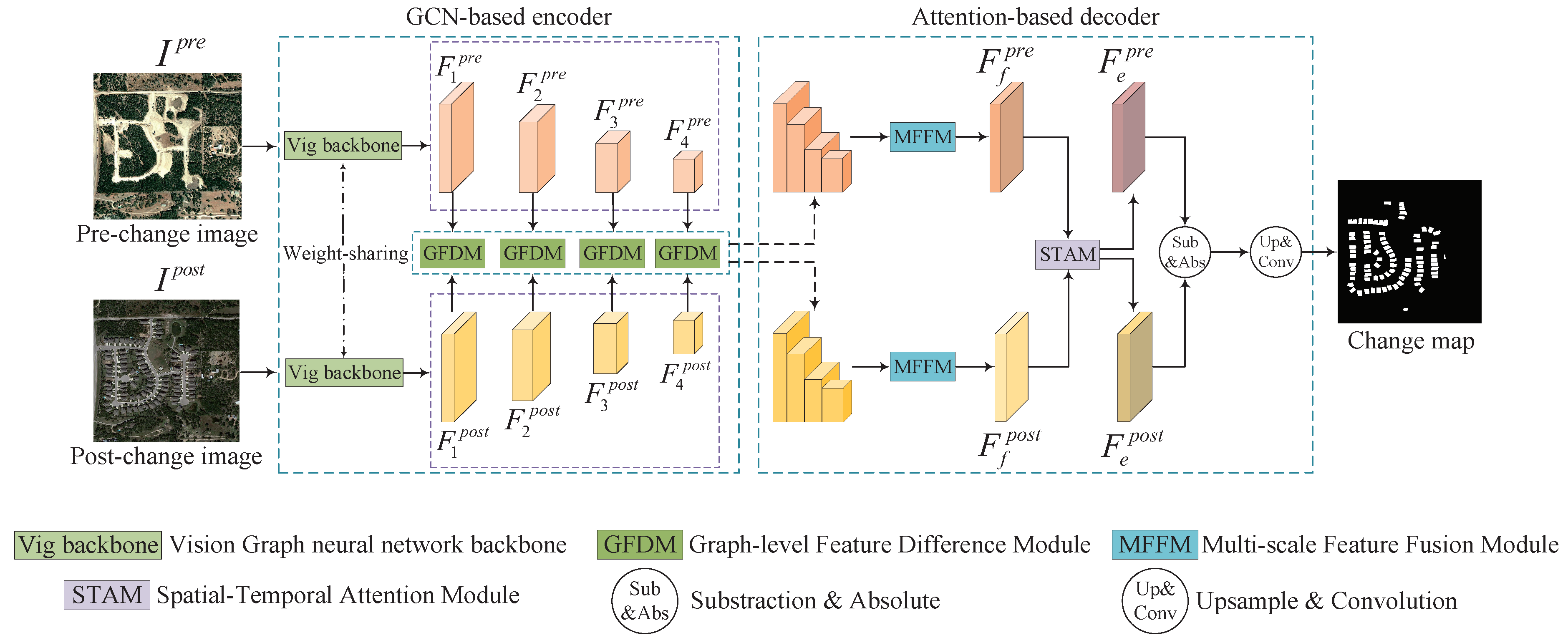
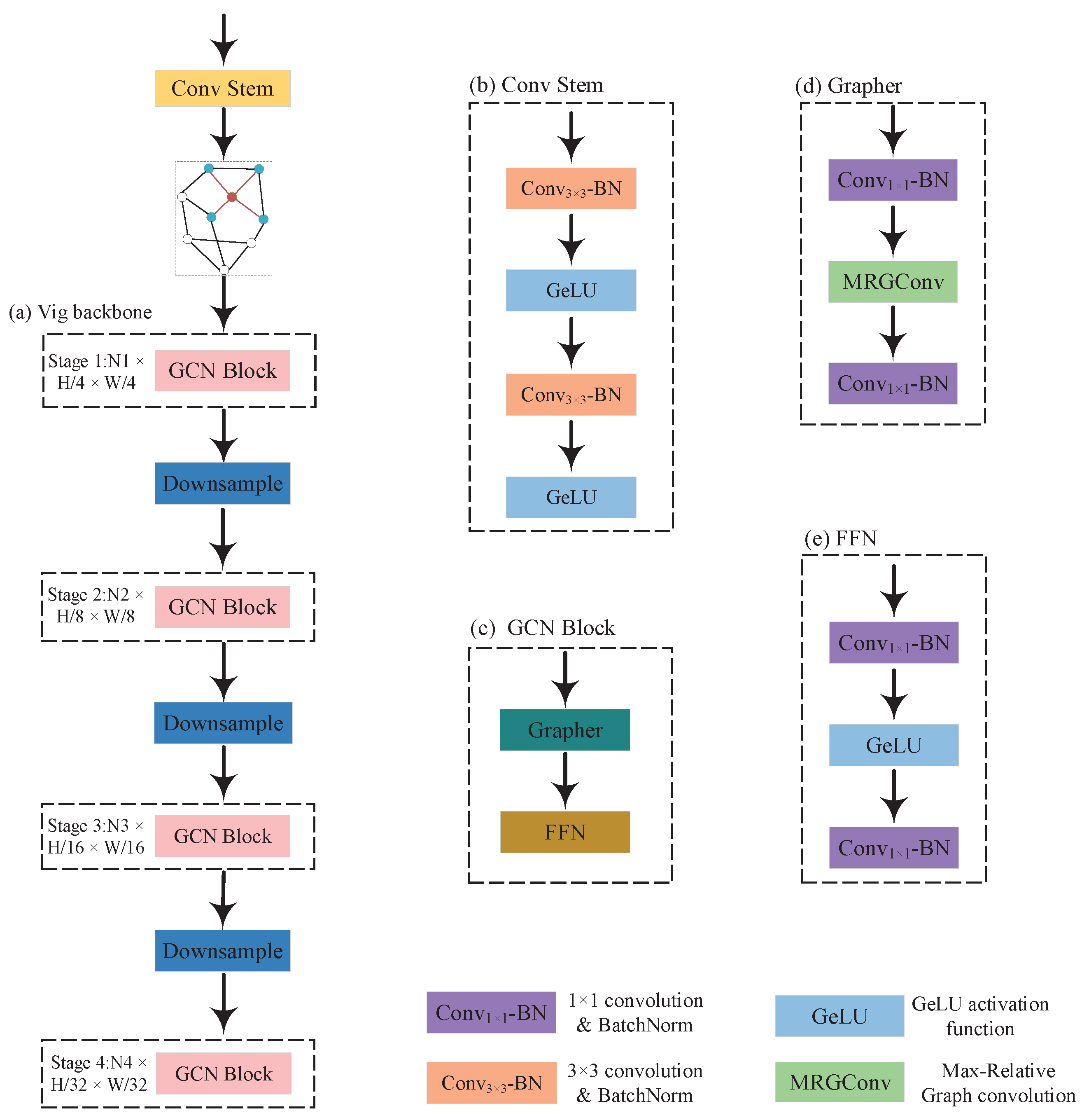
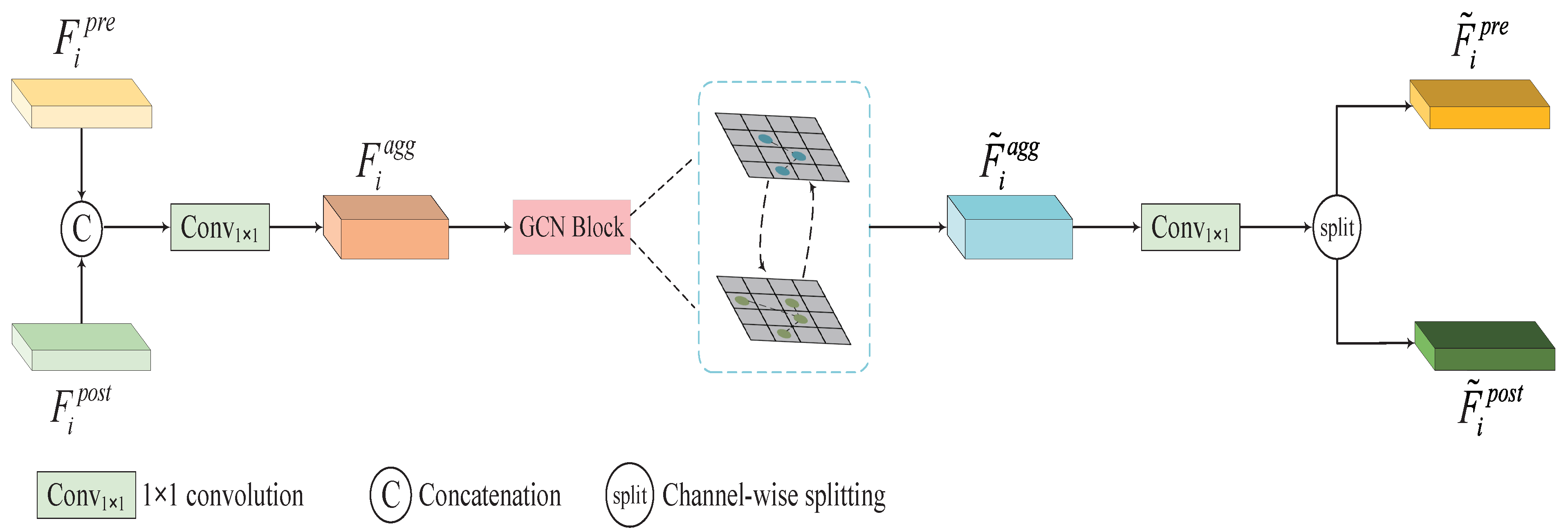
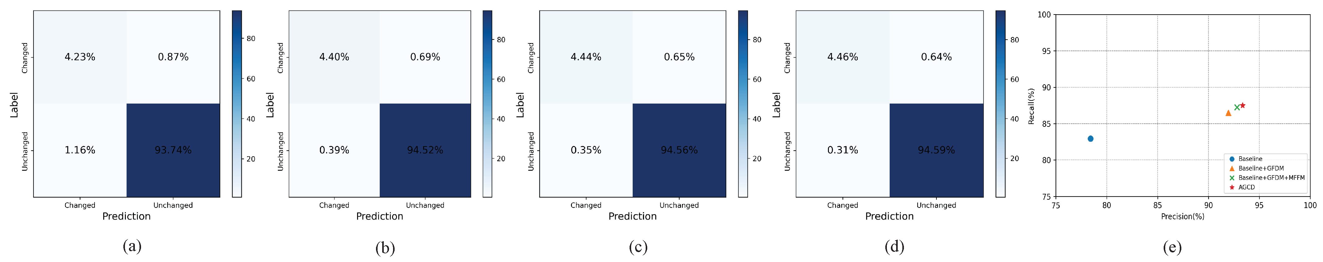
In this article, we put forward AGCD for change detection, which aims to address the challenge of pseudo changes and improve detection accuracy. The motivation for this study stems from the finding that existing methods are susceptible to pseudo changes due to two main reasons: (1) insufficient semantic understanding within individual images and (2) inadequate feature interaction between bitemporal images, which ultimately leads to suboptimal change-detection performance. To address these challenges, AGCD integrates GCN and attention mechanisms into a unified framework, with the following two core objectives: (1) Enhance semantic understanding: To capture nuanced features, AGCD leverages the hierarchical ViG backbone, enabling graph-level feature extraction for detailed representation of individual images. Additionally, MFFM is introduced to synthesize multi-scale features, facilitating comprehensive contextual understanding. (2) Improve bitemporal feature interaction: AGCD promotes effective interaction between features of bitemporal images through the proposed GFDM and STAM. GFDM facilitates multi-scale interactions at the graph level, comprehensively modeling feature similarities and disparities, while STAM employs spatial-temporal attention to enhance the identification of unchanged regions, ensuring accurate classification of changes. The core hypothesis is that our AGCD, with the integration of these modules for refined semantic understanding and enhanced feature interaction, will effectively address the problem of pseudo changes and deliver reliable change-detection results. To validate this hypothesis, extensive experiments on multiple benchmark datasets are conducted to assess both the overall performance of the AGCD and the individual contributions of each proposed module.
The main contributions of this work are summarized as follows:
(1)
We propose a novel change-detection network, namely AGCD, which integrates a GCN-based encoder with an attention-based decoder, aiming at effectively addressing the issue of pseudo changes and enhancing change-detection precision.
(2)
The GCN-based encoder utilizes a weight-sharing ViG backbone to extract hierarchical graph-level features, complemented by a straightforward but efficient module, GFDM, to facilitate graph-level feature interaction, improving the network’s ability to discern differential clues and alleviating the impact of pseudo changes.
(3)
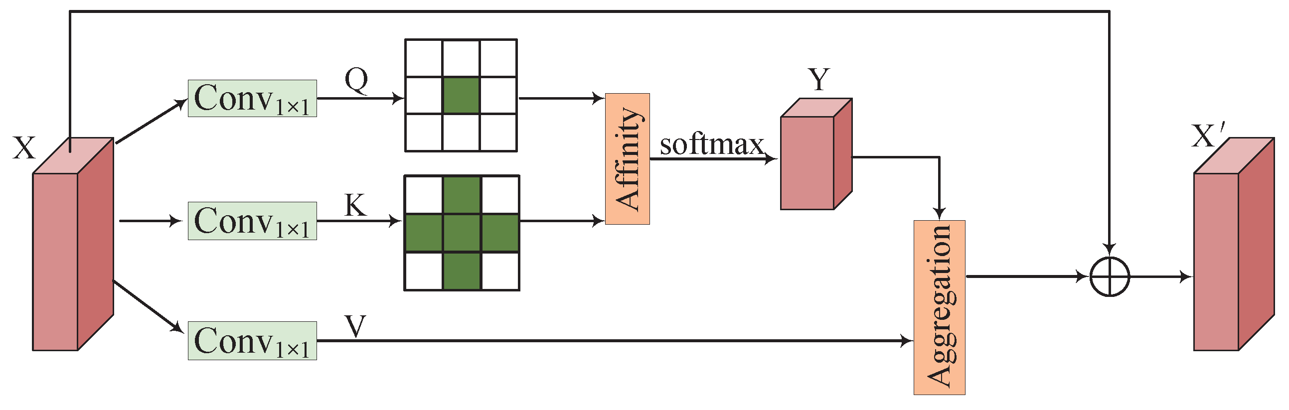
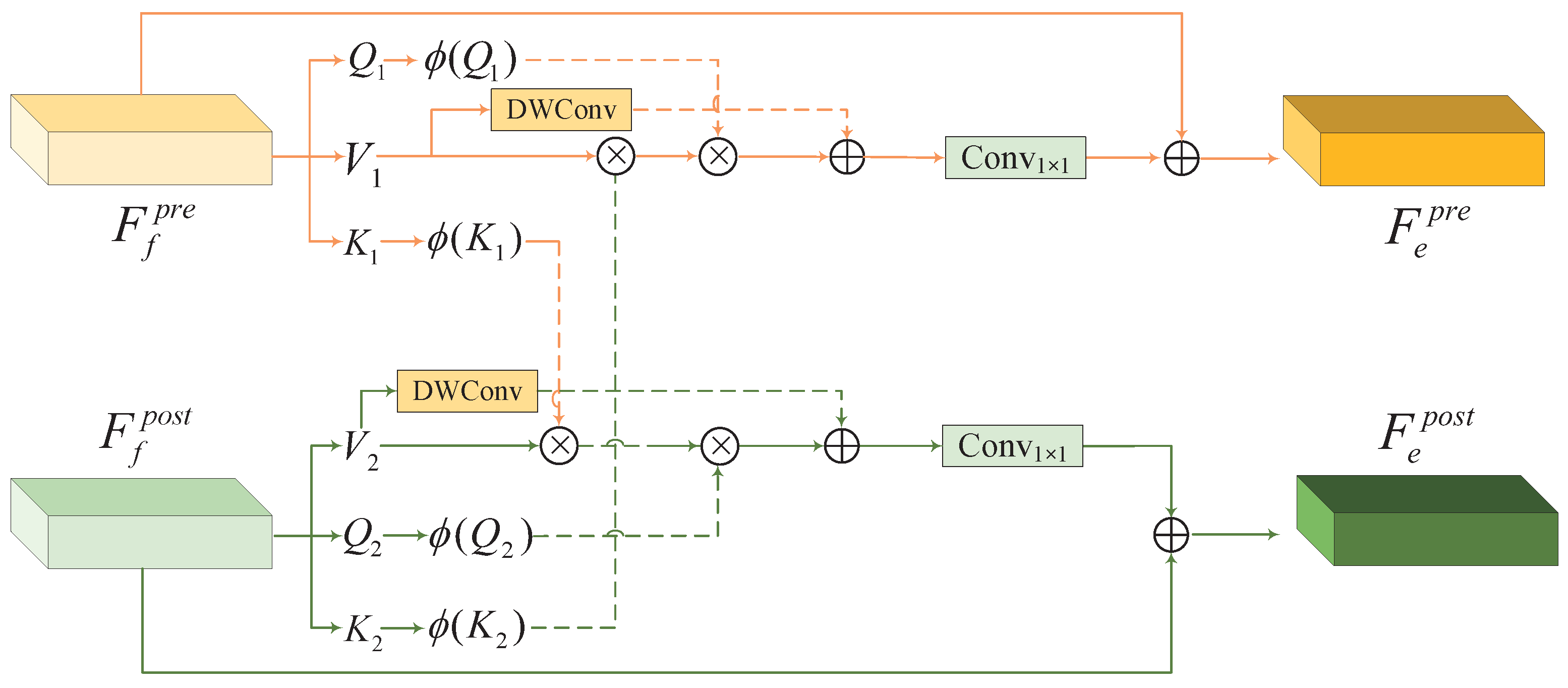
The attention-based decoder consists of MFFM and STAM. MFFM uses criss-cross attention (CCA) to refine multi-scale features, while STAM models spatial-temporal dependencies, enhancing the semantic clarity of change areas and reducing pseudo changes for accurate change detection.

2. Methods

In this section, we first present an overview of the entire framework of AGCD. Then, detailed descriptions of the individual component that constitutes AGCD are provided.

2.1. Overview

Figure 2 shows the overall architecture of AGCD, which is composed of two main components: a hierarchical GCN-based encoder for processing graph-level feature maps and an attention-based decoder for feature enhancement. Specifically, given bitemporal images, the encoder utilizes a weight-sharing ViG backbone to extract multi-scale graph-level features, which capture both local and contextual information. To uncover subtle changes over time, GFDM is designed to facilitate interactions between multi-scale bitemporal features at a graph level, enabling the model to effectively capture both similarities and differences. The attention-based decoder consists of MFFM and STAM. MFFM synthesizes cross-scale feature maps of each image passed by GFDM, empowering the model to discern objects of diverse sizes. This strategic feature fusion across scales is crucial for a holistic understanding of the image content, as it allows the model to embrace both the global semantics and the local details. STAM is devised to model spatial-temporal dependencies of bitemporal features, focusing on unchanged areas and enriching the overall interpretative power of the attention-based decoder. Together, these components work in unison to refine the feature maps, effectively mitigating the influence of pseudo changes and improving the accuracy of change detection. Finally, the whole process culminates in the generation of a pixel-level feature map after a simple processing of the enhanced features.

2.2. GCN-Based Encoder

2.2.1. ViG Backbone

We aim to construct the graph representation G ( V , E ) of bitemporal images, where V and E represent the node and edge set, respectively. We adopt ViG [46] as the foundation of our GCN-based encoder. As showcased in Figure 3, the input bitemporal images first pass through a convolutional stem, generating N feature patches X = { x 1 , x 2 , x 3 , . . . , x N } , each serving as a unique node v i in V. The edge set E is formed by connecting each node v i to its K nearest neighbors N ( v i ) based on feature similarity.
From the perspective of the full graph, the graph convolution operation is implemented by the aggregation and update operations in sequence:
G = U p d a t e ( A g g r e g a t e ( G , W a g g ) , W u p d a t e )
where W a g g and W u p d a t e represent learnable weights for the aggregation and the update operations, respectively. For each individual node within the graph, the process of graph convolution is expressed as:
v i = h ( v i , g ( v i , N ( v i ) ) , W a g g , W u p d a t e )
Here, max-relative graph convolution is adopted for node aggregation. Then:
g ( · ) = v i = [ v i , m a x { v i v j } | v j N ( v i ) ]
h ( · ) = v i = v i W u p d a t e
where [·, ·] indicates channel-wise concatenation.
As illustrated in Figure 3, the ViG backbone consists of four stages, each comprising multiple GCN blocks. Downsampling operations reduce spatial resolution while increasing feature richness between stages. Specifically, the ViG backbone extracts four levels of features F i p r e , F i p o s t , i = 1 , 2 , 3 , 4 from bitemporal images I p r e , I p o s t , respectively. As the network deepens, the ViG backbone progressively refines and distills features, enhancing the model’s ability to uncover the complex patterns embedded within the graph representation. Unlike the grid-like structure of CNNs and the sequence-like structure of Transformers, ViG backbone extracts graph-level features, offering greater flexibility for handling complex objects in remote sensing images and facilitating subsequent graph-level interactions.

2.2.2. Graph-Level Feature Difference Module

GFDM is specifically designed to address the insufficient feature interaction between bitemporal images, which often leads to feature misalignment and pseudo changes. As illustrated in Figure 4, the module first concatenates the bitemporal features extracted from the ViG backbone. A 1 × 1 convolution is applied after concatenation for initial aggregation of information from both temporal phases while also reducing dimensionality, producing F i a g g which preserves both graph-level pre- and post-change contexts. This aggregated feature map is then fed into the GCN block, unlike the GCN block in the ViG backbone, which captures robust semantic features by leveraging regional similarity within individual images. The GCN block in GFDM operates to explicitly enhance feature interactions between the two temporal phases, modeling the cross-temporal relationships between bitemporal features. Specifically, the GCN block in GFDM builds connections based on the similarity between bitemporal feature representations. Regions that remain unchanged tend to have highly similar feature representations across time. Through information propagation across bitemporal features, GCN enhances the semantic consistency of unchanged regions, which in return strengthens the distinction of changed areas. Following this graph-level interaction, the resulting feature map F ˜ i a g g is obtained. F ˜ i a g g first undergoes a 1 × 1 convolution for dimensionality restoration, and then it is split into distinct refined feature maps F ˜ i p r e and F ˜ i p o s t corresponding to the pre- and post-change features, respectively.
The process of GFDM engages in a mathematical formulation outlined as below:
F i a g g = C o n v 1 × 1 ( [ F i p r e , F i p o s t ] )
F ˜ i a g g = G C N B l o c k ( F i a g g )
F ˜ i p r e , F ˜ i p o s t = s p l i t ( C o n v 1 × 1 ( F ˜ i a g g ) ) , i = 1 , 2 , 3 , 4
Here, C o n v 1 × 1 means 1 × 1 convolution, s p l i t ( · ) denotes channel-wise splitting, and G C N B l o c k ( · ) represents the GCN block used in ViG backbone.
GFDM is independently applied to feature maps at different scales. This multi-scale graph-level interaction mechanism ensures that bitemporal features at various scales are adaptively aligned across time, effectively capturing both large-scale and fine-grained similarities and distinctions. By optimizing feature interactions at multiple levels, GFDM mitigates feature misalignment, provides better-aligned features for downstream fusion, and reduces pseudo changes, ultimately improving change-detection accuracy.

2.3. Attention-Based Decoder

2.3.1. Multi-Scale Feature Fusion Module

Following GFDM in the GCN-based encoder, we obtain four levels of feature maps, denoted as F ˜ i p r e , F ˜ i p o s t , i = 1 , 2 , 3 , 4 , which encapsulate spatial and channel-wise information at across different scales. This four-level hierarchy follows the convention of modern vision backbones [47,48] to optimally balance multi-scale representation and computational efficiency. Empirically, Low-level, high-resolution feature maps preserve local details, while high-level, low-resolution maps focus on global semantics. Inspired by previous works [22,49,50,51], we integrate CCA [52] and CBAM [53] by leveraging their complementary properties. Specifically, CCA is applied to high-level feature maps to model long-range dependencies and enrich global semantic understanding, whereas CBAM refines spatial and channel-wise representations to preserve critical local details for precise change detection. While both modules have been widely utilized individually in prior studies, their joint utilization in our framework allows us to effectively combine their strengths for improved feature integration. Since comprehensive information from each image is essential for aligning features and discerning changes between bitemporal images, MFFM plays a key role in mitigating pseudo changes and enhancing performance. Take F ˜ i p r e for example, this process can be mathematically expressed as follows:
F ^ k p r e = C o n v 3 × 3 ( [ C B A M ( F ˜ k p r e ) , C C A ( F ˜ k p r e ) ] , k = 2 , 3 , 4
where F ^ k p r e denote high-level semantic feature maps, C o n v 3 × 3 signifies a 3 × 3 convolution layer. Although coarse-grained feature maps are rich in contextual semantics, they lack local features. We enhance the coarse-grained global semantics with local features to derive a refined feature map in more detail, which could be expressed as:
F f p r e = C o n v 1 × 1 ( [ ( σ ( F ˜ 1 p r e ) + I ) · U p ( F ˜ 2 p r e ) , ( σ ( F ˜ 1 p r e ) + I ) · U p ( F ˜ 3 p r e ) , ( σ ( F ˜ 1 p r e ) + I ) · U p ( F ˜ 4 p r e ) ] )
where F f p r e of size H / 4 × W / 4 × C 4 represents the fused feature map for pre-change image, U p ( · ) refers to upsampling operation, I means identity matrix, and σ denotes softmax function. CCA was not applied to the lowest-level feature map, as long-range dependencies are less critical for low-level features. The analogous process for the post-change scenario yields F f p o s t in a manner reflective of its pre-change counterpart. This approach empowers our attention-based decoder to capture the intricate details and broader context within the images. The above process of MFFM is depicted in Figure 5.
As depicted in Figure 6, CCA effectively encapsulates both vertical and horizontal contextual correlations via processes of affinity computation and aggregation. Upon receiving an input tensor X R H × W × C , CCA employs a 1 × 1 convolution layer to generate both a query map Q and a key map K, each with dimensions H × W × C , where C = C / 8 represents a reduced channel dimension. For a given position u within Q, the horizontally and vertically aligned vectors at the corresponding position in K form a collective set Ω u R ( H + W 1 ) × C . Subsequently, CCA calculates the affinity matrix Y R ( H + W 1 ) × ( H × W ) to quantify these relationships:
Y = σ ( d i , u ) = σ ( Q u Ω i , u T )
Here, d i , u quantifies the affinity between Q u and the i-th element Ω i , u of the set Q u . The vector Q u R C represents the query features at a given location u. In parallel, V R H × W × C is generated from input X via 1 × 1 convolution. The aggregation process subsequently amalgamates these features to produce the refined feature set X , expressed as:
X u = i Φ u Y i , u Φ i , u + X u
where X u refers to the feature vector at each position u in the enhanced map X . Y i , u is the normalized affinity at the i-th channel and position u within the affinity matrix Y. Φ u is the feature vector extracted from V at position u, and Φ i , u corresponds to the i-th element of this vector.

2.3.2. Spatial-Temporal Attention Module

During the feature-fusion process, misalignment between multi-scale features can lead to inevitable distortion, which may disrupt the correspondence between bitemporal features and consequently affect the accurate identification of changed regions. To minimize the loss of correspondence, we have developed STAM, which harnesses focused linear cross-attention [54] for modeling spatial-temporal inter-dependencies inherent in bitemporal features. The architectural schema of STAM is depicted in Figure 7.
STAM initiates its process by receiving the fused bitemporal feature maps from MFFM. It projects the bitemporal features F f p r e into Query Q 1 , Key K 1 , and Value V 1 . Analogously, it applies the same projection to F f p o s t to obtain Q 2 , K 2 , and V 2 , then the cross affinity between F f p r e and F f p o s t is gauged via a vanilla cross-attention calculus, delineated as follows:
S 1 = Q 1 × K 2 T
S 2 = Q 2 × K 1 T
Focused linear cross-attention employs a carefully designed kernel as the approximation of the original similarity function, then Formulas (12) and (13) could be rewritten to obtain the linear cross affinity between F f p r e and F f p o s t :
S 1 = ϕ p ( Q 1 ) × ϕ p ( K 2 ) T
S 2 = ϕ p ( Q 2 ) × ϕ p ( K 1 ) T
where:
ϕ p ( x ) = f p ( R e L U ( x ) )
f p ( x ) = | | x | | | | x * * p | | x * * p
Here, f p denotes a mapping function tailored to modulate the directional alignment of query and key features and foster convergency of similar query–key pairs while diverging dissimilar counterparts. The notation x * * p signifies an element-wise exponentiation to the power of p (default set to 3). Subsequently, the enhanced feature map is obtained through the following formulation:
F e p r e = F f p r e + C o n v 1 × 1 ( ϕ p ( Q 1 ) × ( ϕ p ( K 2 ) T × V 1 ) ) + D W C o n v ( V 1 )
F e p o s t = F f p o s t + C o n v 1 × 1 ( ϕ p ( Q 2 ) × ( ϕ p ( K 1 ) T × V 2 ) ) + D W C o n v ( V 2 )
where D W C o n v ( · ) denotes depth-wise convolution [55] used to maintain feature diversity. With the integration of this refined attention mechanism, STAM could fully capture complex spatial-temporal relationship between bitemporal features, improving the certainty of the change pixel. Ultimately, the process culminates in the generation of the predicted change map:
C h a n g e m a p = C o n v 1 × 1 ( U p ( | F e p o s t F e p r e | ) ) .

3. Datasets and Experimental Settings

In this subsection, three benchmark datasets employed in our experiments are introduced first. Then, the implementation details and evaluation metrics are provided. Finally, the comparative methods are briefly described.

3.1. Dataset Descriptions

We carried out our experiments on three renowned public datasets, the LEVIR-CD dataset [56], the WHU-CD dataset [57], and the SYSU-CD dataset [22].
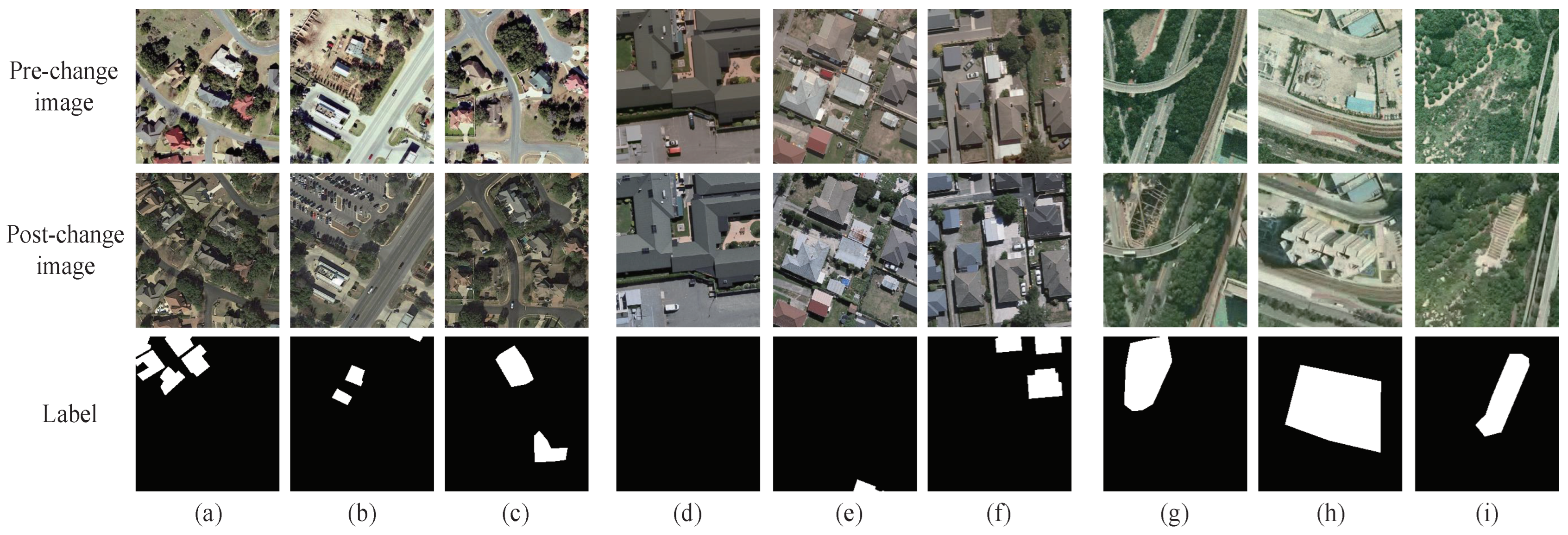
The LEVIR-CD is composed of 637 pairs of high-resolution images, each measuring 1024 × 1024 pixels. These images, taken over a span of 5 to 14 years, illustrate a wide range of urban changes, including building construction and demolition. The dataset includes 31,333 instances of building alterations. For our study, we cropped the original image pairs to a size of 256 × 256 pixels and split the dataset into training, validation, and testing sets containing 7120, 1024, and 2048 pairs, respectively.
The WHU-CD dataset contains two high-resolution aerial images, each with a resolution of 0.075 m and dimensions of 32,507 × 15,354 pixels. These images record the urban development in Christchurch, New Zealand, from 2012 to 2016, with a focus on building structure changes. In our experiments, we extracted non-overlapping 256 × 256 patches from these images and organized the dataset into training, validation, and testing subsets, which include 6096, 762, and 762 pairs, respectively.
The SYSU-CD dataset offers a comprehensive set of 20,000 pairs of very high-resolution aerial images, each with a 0.5 m resolution and originally sized at 256 × 256 pixels. It captures a spectrum of intricate urban changes in Hong Kong between 2007 and 2014, encompassing the rise of new structures and the broadening of roadways. For our analysis, we allocated the dataset into training, validation, and testing segments, comprising 7120, 1024, and 2048 pairs, respectively.
Examples of the three datasets are shown in Figure 8.

3.2. Implementation Details

We constructed our model utilizing the PyTorch 1.11.0 framework and trained it on a single NVIDIA Tesla V40 GPU. Standard data-augmentation techniques are employed on the input image, including random flipping and random rotating. In terms of model optimization, we employ the AdamW optimizer. The decay rates for the estimation of the first and second moments are set to their default values of 0.9 and 0.999, respectively. The weight decay is configured to 0.01. The initial learning rate is carefully chosen to be 0.0005, 0.0002, and 0.0006 for LEVIR-CD, WHU-CD, and SYSU-CD datasets, respectively. The batch size and the number of epochs for training are set to 32 and 100, respectively.

3.3. Evaluation Metrics

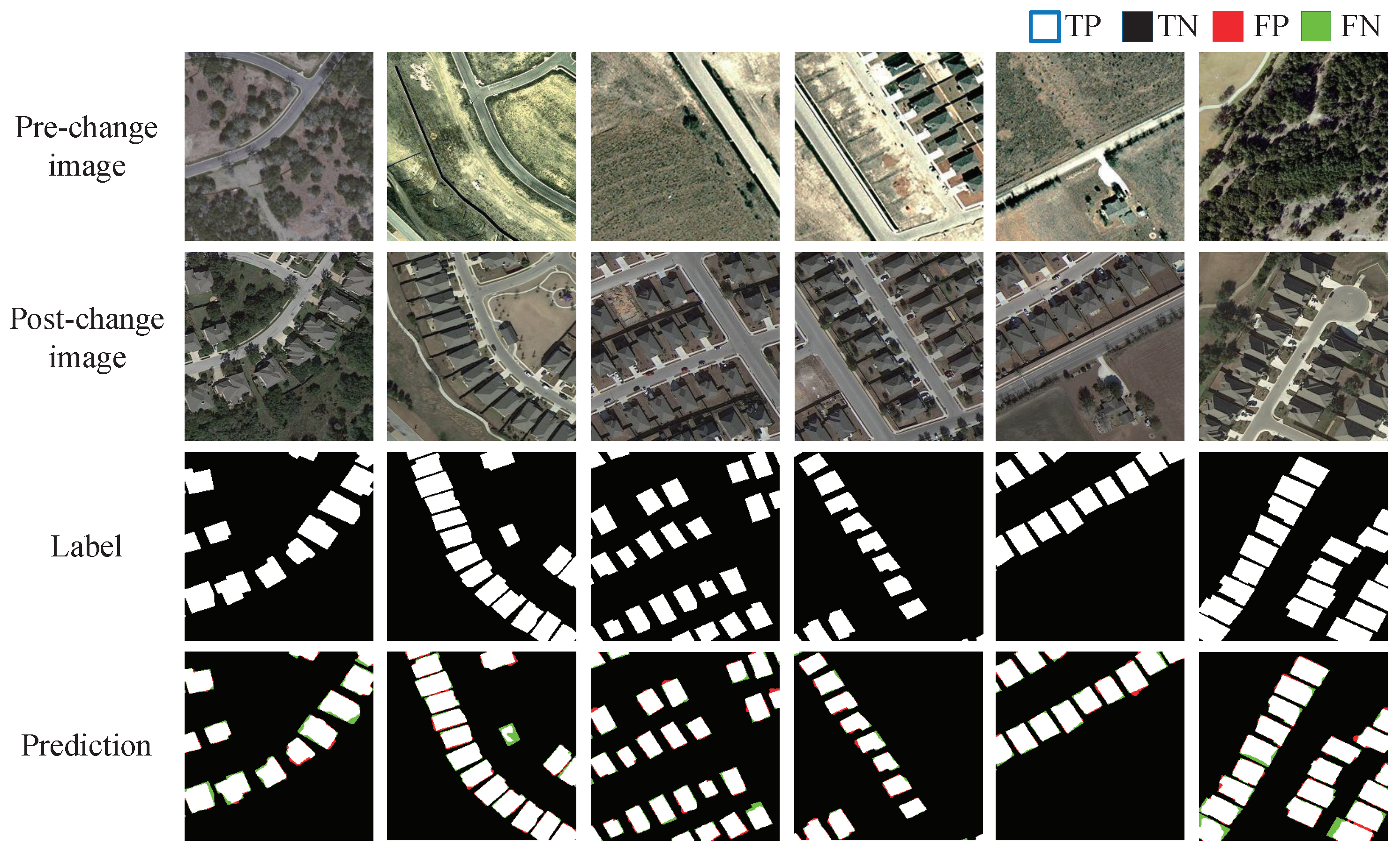
In our experiment, we selected precision (Pre), recall (Rec), F1-score (F1), overall accuracy (OA), and intersection over union (IoU) as the main evaluation indices. The definitions of these metrics are as follows:
P r e = T P T P + F P
R e c = T P T P + F N
I o U = T P T P + F N + F P
O A = T P + T N T P + T N + F N + F P
F 1 = 2 · P r e · R e c P r e + R e c
where TP, FP, TN, and FN represent the number of true positive (TP), false positive (FP), true negative (TN), and false negative (FN), respectively.

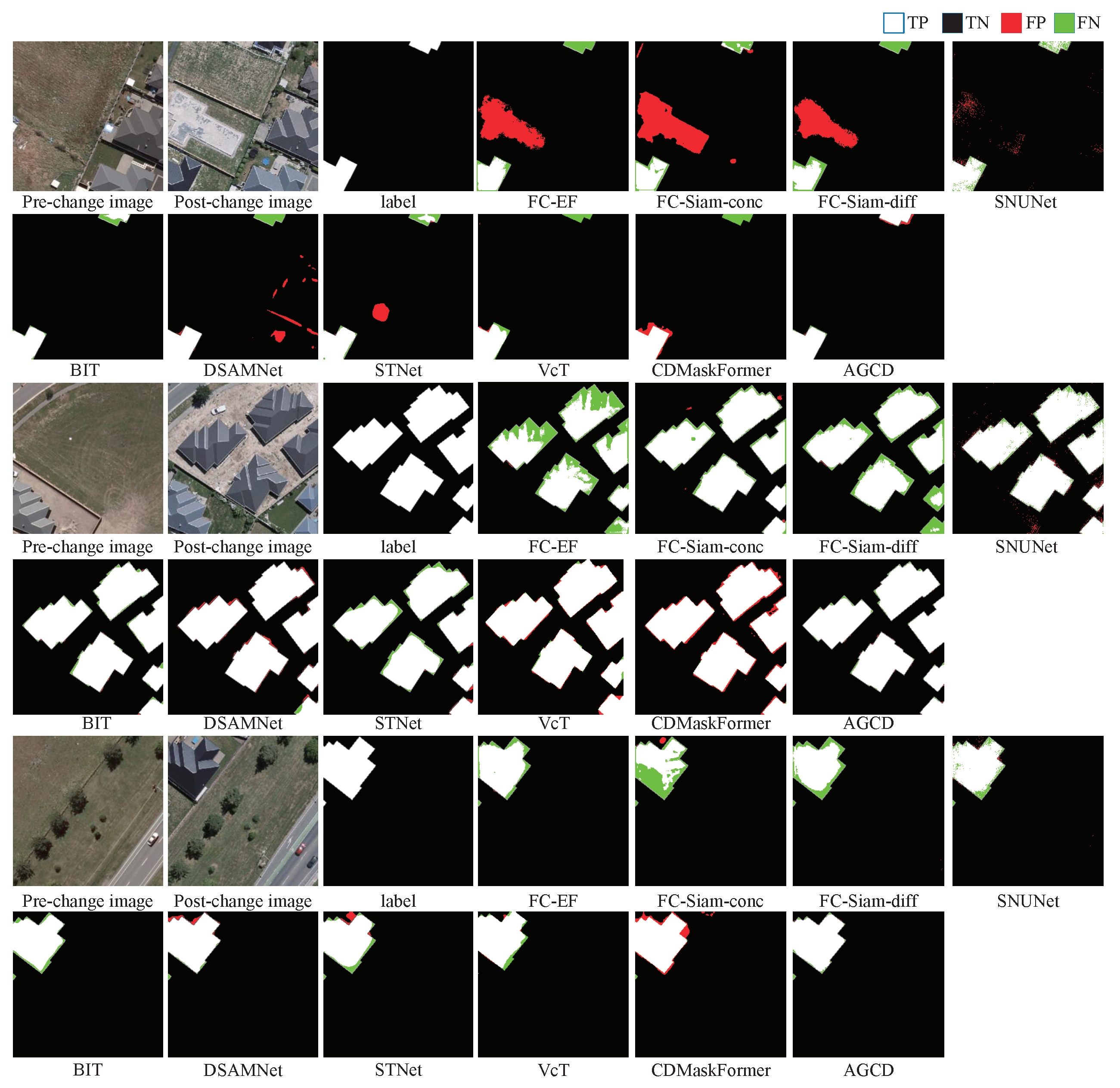
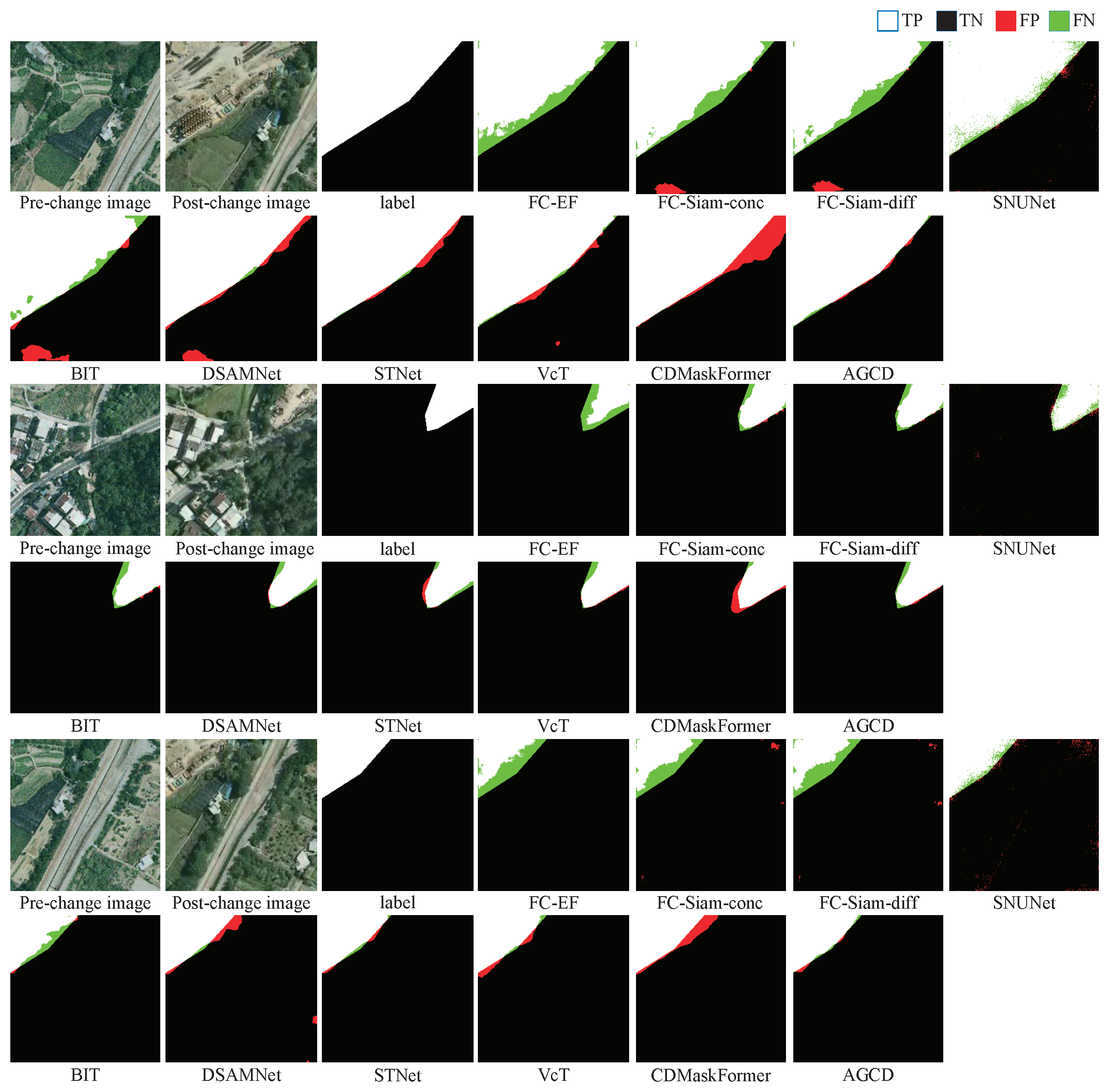
3.4. Comparative Methods

AGCD was compared to several state-of-the-art models to verify its effectiveness, including FC-EF [20], FC-Siam-conc [20], FC-Siam-diff [20], SNUNet [58], BiT [28], DSAMNet [22], STNet [59], VcT [40], and CDMaskFormer [60].
  • FC-EF, FC-Siam-conc, and FC-Siam-diff: Three variants of FCNs used for change-detection tasks. FC-EF combines bitemporal images along the channel axis before they are passed into the network. FC-Siam-conc employs a siamese network for bitemporal feature extraction, which are then fused. FC-Siam-diff, also using a siamese network, extracts bitemporal features and applies their absolute differences to capture differential clues.
  • SNUNet: Inspired by UNet++, SNUNet employs dense connection between bitemporal features to reduce semantic gaps and localization errors, resulting in more accurate change maps.
  • BiT: A lightweight network for change detection that converts bitemporal features into semantic tokens, facilitating context modeling and information exchange in a compact, token-based space–time framework.
  • DSAMNet: DSAMNet introduces parallel convolutional blocks to refine features, addressing feature misalignment and inefficient supervision.
  • STNet: STNet combines spatial and temporal features using cross-temporal and cross-scale mechanisms to recover fine spatial details, improving change-detection accuracy.
  • VcT: A hybrid method combining GCN and Transformer, which leverages GCN to refine token representations extracted from bitemporal images for reliable change detection.
  • CDMaskFormer: CDMaskFormer utilized a Transformer-based decoder for interaction of features passed from a well-designed change extractor. Change prototypes derived from this decoder are then normalized to generate the final change map.

4. Results

Here, we report the performance of AGCD and comparative methods, as well as the ablation study results for each component.

4.1. Performance Comparisons

4.1.1. Comparison on LEVIR-CD Dataset

As shown in Table 1, the quantitative analysis on the LEVIR-CD dataset reveals that FC-EF, FC-Siam-conc, and FC-Siam-diff perform poorly across all metrics, ranking at the bottom among the comparative methods. CDMaskFormer achieves the highest recall score of 89.59%, highlighting its ability to effectively reduce missed detections. AGCD achieves the highest precision of 93.36%, demonstrating its strong capability in minimizing pseudo change misidentification. Moreover, AGCD excels in overall performance, achieving the highest scores in IoU and F1-score. Specifically, it surpasses the second-best method, VcT, with a 0.30% improvement in F1-score and a 0.49% increase in IoU. These results underscore AGCD’s competitive performance over current state-of-the-art methods.
The visualization analysis of different methods on the LEVIR-CD dataset is shown in Figure 9, and the examples of AGCD’s predictions are displayed in Figure 10. FC-EF generates numerous pseudo changes between the two buildings, while VcT and CDMaskFormer introduce pseudo changes along the edges of the buildings. In contrast, STNet and AGCD demonstrate superior performance by accurately detecting the complete change regions with minimal pseudo changes. In the second example, FC-EF, FC-Siam-conc, and FC-Siam-diff fail to capture most change areas, whereas STNet and CDMaskFormer detect building changes but generate pseudo changes at building junctions. Due to the spectral similarity between target building change regions and adjacent unchanged areas, VcT’s spatial neighborhood aggregation degrades local discriminative characteristics, resulting in numerous missing detections of changed areas. In contrast, AGCD not only detects the change areas as completely as possible but also notably reduces pseudo changes. The third example reveals that although FC-EF avoids pseudo changes, it misses many genuine changes. DSAMNet consistently exhibits pseudo changes near building boundaries or junctions. AGCD, however, outperforms other methods by effectively minimizing pseudo changes and capturing more complete building change contours.

4.1.2. Comparison on WHU-CD Dataset

The quantitative analysis on WHU-CD dataset is presented in Table 2 presents. FC-Siam-diff demonstrates the lowest F1-score at 51.92%, followed by FC-Siam-conc with an F1-score of 63.60%. The suboptimal performance of these methods can be attributed to their reliance on simple concatenation or difference operations, which inadequately model feature interactions and fail to capture spatial-temporal dependencies in complex scenarios. CDMaskFormer achieves the highest recall score of 92.81%. Benefiting from the integration of GCN and attention mechanism, AGCD outperforms all competing methods across multiple metrics. Specifically, it surpasses the second-best performer, CDMaskFormer, by notable margins: 2.70% in F1-score and 3.24% in IoU. Futhermore, AGCD achieves the highest precision score of 93.07%, which underscores its enhanced capability to minimize false positives and effectively mitigate the interference of pseudo changes.
The visualization analysis on the WHU-CD dataset is shown in Figure 11, and the examples of AGCD’s predictions on WHU-CD dataset are presented in Figure 12. Across all three examples, FC-EF, FC-Siam-conc, and FC-Siam-diff exhibit significant limitations, either introducing substantial pseudo changes or failing to detect many actual change regions. In the first case, CDMaskFormer introduces pseudo changes along the edges of buildings and fails to detect small building changes. In the second and third examples, although DSAMNet and CDMaskFormer successfully identify true change regions, they still produce continuous pseudo changes near the boundaries of the detected areas. In contrast, BIT and AGCD demonstrate superior performance by effectively minimizing pseudo changes while accurately delineating change regions with well-defined contours.

4.1.3. Comparison on SYSU-CD Dataset

Based on the quantitative results on the SYSU-CD dataset in Table 3, CDMaskFormer achieves the highest recall of 85.87%, followed by DSAMNet (83.32%), indicating their strong ability to identify the majority of actual change regions with minimal omission. On the other hand, STNet achieves the best precision of 84.77%, with AGCD close behind at 84.75%, highlighting their effectiveness in minimizing false positives and resisting pseudo change interference. While STNet excels in precision and CDMaskFormer leads in recall, AGCD stands out with its comprehensive performance across multiple metrics, effectively balancing true positive detection and false positive reduction. Specifically, AGCD achieves the highest scores in IoU (67.79%), F1-score (80.80%), and OA (91.35%). Overall, the quantitative outcomes demonstrate AGCD’s competitive edge compared to other advanced methods.
The visualization analysis of the comparative methods on the SYSU-CD dataset and the examples of AGCD’s predictions on this dataset are shown in Figure 13 and Figure 14, respectively. Overall, FC-EF fails to detect many change regions, while FC-Siam-conc and FC-Siam-diff not only miss numerous change areas but also introduce some pseudo changes. Although CDMaskFormer detects most change regions, it introduces noticeable pseudo changes along the edges of the detected areas. In contrast, AGCD exhibits fewer errors and more accurately delineates the change boundaries. Overall, AGCD stands out with its competitive performance, as it strikes a balance between minimizing false positives and capturing more true changes.

4.2. Ablation Study

In this subsection, an ablation study is conducted on three public datasets to validate the contribution of each key component in AGCD. We constructed the baseline model by removing GFDM and STAM and replacing MFFM by a simple CNN-based feature-fusion module.

4.2.1. Ablation Study on LEVIR-CD Dataset

As depicted in Table 4, the baseline model achieves 80.60% in F1-score and 67.51% in IoU on the LEVIR-CD dataset. The introduction of GFDM boosts AGCD’s performance, improving the F1-score to 89.14% and the IoU to 80.42%. This improvement demonstrates GFDM’s ability to promote multi-scale interactions at the graph level, enabling the extraction of more discriminative features and effectively mitigating pseudo changes, as evidenced by the marked reduction in false positives in the confusion matrix (Figure 15). Building upon this, the inclusion of MFFM further boosts AGCD’s performance, with a 0.80% increase in F1-score and a 1.29% improvement in IoU. Finally, the complete AGCD, incorporating all three modules, exhibits the fewest false positives and delivers the highest F1-score (90.34%) and IoU (82.38%). The Pre. vs. Rec. graph illustrates a steady improvement in the model’s performance with the addition of each module. These experimental results clearly demonstrate the contributions of GFDM, MFFM, and STAM to the effectiveness of AGCD.
The visualization analysis of the ablation study on the LEVIR-CD dataset is portrayed in Figure 16. Due to the lack of effective bitemporal feature interaction, the baseline model is susceptible to pseudo change interference. Particularly in the first example, even minor spectral value shifts in buildings caused by lighting condition variations or seasonal changes can lead the baseline model to misclassify these unchanged building regions as changed areas. The integration of GFDM reduces these pseudo changes, effectively suppressing both large-scale misdetections and isolated spots. The addition of MFFM further diminishes pseudo changes, while the full AGCD sharpens the delineation of change contours, enhancing detection precision and highlighting the contributions of all three modules.

4.2.2. Ablation Study on WHU-CD Dataset

As can be seen in Table 5, the baseline model records an F1-score of 84.26% and an IoU of 72.80%. The addition of GFDM notably improves these metrics, elevating the F1-score to 89.60% and the IoU to 81.17%. As shown in the confusion matrix (Figure 17), GFDM effectively reduces false positives (from 0.64% to 0.48%), demonstrating its capability to mitigate pseudo change misdetections. Further improvements are observed with the introduction of MFFM, which reduces false positives to 0.34% while slightly decreasing recall due to more stringent pseudo change filtering. The complete AGCD, incorporating STAM, achieves the highest performance across all metrics. The progressive improvement demonstrates the modules’ collective contributions to the robustness of AGCD.
Figure 18 illustrates the visualization results of our ablation study on the WHU-CD dataset. The baseline model exhibits numerous pseudo change spots and demonstrates poor detection performance along building edges. The incorporation of GFDM effectively reduces false detections while enhancing boundary delineation accuracy. Subsequent integration of MFFM yield further enhancements, effectively suppressing pseudo changes. Finally, the full AGCD achieves the most impressive reduction in pseudo changes, presents more complete change contours, and demonstrates superior overall performance.

4.2.3. Ablation Study on SYSU-CD Dataset

Table 6 delineates the quantitative outcomes of the ablation study on the SYSU-CD dataset. The baseline model garners an F1-score of 72.74% and an IoU of 56.82%. Notably, the false positive rate is observed to be 5.81% for the baseline model. The introduction of GFDM, which enhances feature interaction, leads to a remarkable reduction in false positives to 4.43%, alongside an improvement of 7.60% in IoU and 5.89% in F1-score. The integration of MFFM further refines feature fusion, resulting in a decrease in false positives to 3.81%. Finally, the complete AGCD, incorporating all modules, achieves the minimum false positive rate of 3.28% (Figure 19), alongside the highest F1-score of 80.80% and IoU of 67.79%. The Pre. vs. Rec. graph further demonstrates a progressive increase in precision, while recall shows a slight decrease after the inclusion of MFFM. Despite this, the overall accuracy of change detection is enhanced, highlighting the effectiveness of these modules in progressively reducing the interference of pseudo changes.
The visualization analysis of our ablation study on the SYSU-CD dataset is presented in Figure 20, offering a detailed examination of each module’s contribution to improving AGCD’s performance. The baseline model demonstrates poor detection performance, manifested as continuous false positives along the edges and large patches of pseudo change areas. With the introduction of GFDM, a marked reduction in false positives is achieved, highlighting its effectiveness in suppressing pseudo changes. The subsequent integration of MFFM and STAM further enhances the results, not only reducing pseudo changes but also progressively refining the contours of change regions. Ultimately, the complete AGCD delivers more precise change contours, demonstrating superior detection accuracy and robustness.

4.3. Model Complexity

Table 7 showcases the performance and complexity across different models. The runtime represents the average training time per epoch, calculated over 100 epochs, while the inference time is measured on a single image with a size of 256 × 256. Lightweight models such as FC-EF, FC-Siam-conc, and FC-Siam-diff, with a low parameter count of 1.35 M and GFLOPs ranging from 3.57 to 5.32, exhibit faster runtime and inference time. However, their performance on both datasets lags behind other methods. BIT achieves a commendable balance between complexity and accuracy, with a parameter count of 11.47 M and an F1-score of 88.16% on LEVIR-CD. On WHU-CD, it maintains strong performance with an F1-score of 84.28%. DSAMNet shows commendable performance on both datasets, achieving an F1-score of 88.23% on LEVIR-CD and 83.94% on WHU-CD. However, it is computationally intensive, requiring 75.39 GFLOPs and 647 s per epoch for training on LEVIR-CD, and 536 s per epoch on WHU-CD. In contrast, AGCD, with 36.35 M parameters and 15.22 GFLOPs, delivers substantial performance improvements. While this involves a modest increase in the number of parameters, the trade-off is justified by its noteworthy gains in model performance. Specifically, AGCD achieves the highest IoU and F1-score on both LEVIR-CD and WHU-CD datasets. On WHU-CD, AGCD surpasses the second-best model, CDMaskFormer, by a notable margin of 2.70% in F1-score. Regarding runtime, AGCD requires 476 s and 400 s per epoch for training on LEVIR-CD and WHU-CD, respectively. Compared to CDMaskFormer and VcT, AGCD achieves superior performance with a moderate increase in training and inference time.
In summary, AGCD strikes an optimal balance between complexity and performance. With a moderate increase in parameters and computational cost, AGCD notably improves IoU and F1-score, outperforming both lightweight and high-complexity models.

4.4. Feature Visualization

The feature visualization of AGCD is presented in Figure 21. Without GFDM processing, the bitemporal feature maps struggle to clearly highlight potential change regions, resulting in poor focus on areas of interest. After applying GFDM, the feature maps begin to concentrate more on the change regions, gradually shifting focus towards potential changed areas. With the implementation of MFFM, the feature maps further enhance the representation of change regions while suppressing irrelevant information. Finally, the introduction of STAM strengthens the model’s focus to change areas, demonstrating a more pronounced suppression of unchanged areas and a clearer emphasis on the change regions. This progression clearly shows that our proposed modules, GFDM, MFFM, and STAM, work together to gradually suppress the distracting information and direct the entire network’s attention towards the change regions.

5. Discussions

In this paper, extensive experiments across three benchmark datasets, LEVIR-CD, WHU-CD, and SYSU-CD, are conducted to rigorously verify the effectiveness of our proposed AGCD. The quantitative outcomes of these experiments demonstrated AGCD’s competitive or even superior performance over cutting-edge approaches in change-detection tasks. AGCD’s resistance against pseudo changes exhibited in the visualization results is particularly noteworthy, as it provides more reliable results compared to comparative methods. Additionally, compared to other methods, AGCD excels in maintaining the integrity of edge detection within change areas, including both large-scale areas and small targets. The ablation study we conducted further substantiates the contribution of the three components we introduced. Notably, GFDM remarkably improves AGCD’s performance, highlighting the pivotal role of GCN in enabling cross-temporal interaction for multi-scale bitemporal features. By modeling complex spatial relationships through graph-based interactions, GFDM effectively aligns bitemporal features and reduces pseudo changes caused by imaging inconsistencies.

6. Conclusions

In summary, this study presents AGCD, a novel attention-guided graph neural network designed to reduce pseudo changes and enhance change detection in remote sensing images. The innovative integration of GCN with an attention mechanism empowers AGCD to effectively model spatial-temporal relationships and to promote feature interactions, resulting in a more precise and enhanced change detection. AGCD’s architecture is a well-coordinated combination of three key components: GFDM, MFFM, and STAM. These modules work together to resolve two key challenges: the limited understanding of semantic information in individual images and insufficient information exchange between bitemporal images. GFDM facilitates comprehensive feature interactions, enhancing the capture of similarity between unchanged regions, which in turn improves the model’s ability to distinguish changes. Meanwhile, MFFM ensures effective integration of multi-scale features and STAM focuses on capturing the complex spatial-temporal relationships. The ablation study highlights the contributions of each module in enhancing the model’s performance. Compared to existing state-of-the-art methods, AGCD substantially reduces the misclassification of pseudo changes and outperforms other models across multiple metrics on three benchmark datasets, demonstrating its robustness and effectiveness in change detection. While AGCD has demonstrated competitive or even superior performance compared to existing methods, it still faces several challenges. Specifically, while AGCD achieves notable precision, indicating its strong ability to suppress pseudo changes, its recall is not optimal. This may be attributed to the strict filtering of pseudo changes, which could lead to the omission of certain change regions. Moreover, although we utilized MFFM to fuse multi-scale features, it may tend to overly focus on global semantics, which can lead to the neglect of local details and result in boundary distortions. Future research will explore frequency domain techniques, such as Fourier Transform (FFT) and wavelet transform, to enhance edge localization and capture subtle changes. By integrating these techniques, we aim to improve the model’s ability to accurately detect changes in scenarios with small targets and fine details.

Author Contributions

Conceptualization, H.L., X.L. (Xin Lyu) and X.L. (Xin Li); methodology, H.L.; validation, H.L., S.C. and C.L.; formal analysis, H.L.; writing—original draft preparation, H.L.; writing—review and editing, H.L., X.L. (Xin Lyu), X.L. (Xin Li), Y.F., Z.X., X.W. and C.Z.; visualization, C.X.; supervision, X.L. (Xin Lyu); funding acquisition, X.L. (Xin Lyu) and X.L. (Xin Li). All authors have read and agreed to the published version of the manuscript.

Funding

This research was funded by the National Natural Science Foundation of China (Grant No. 62401196) and Natural Science Foundation of Jiangsu Province (Grant No. BK20241508).

Data Availability Statement

The LEVIR-CD, WHU-CD and SYSU-CD datasets are openly available at https://aistudio.baidu.com/datasetdetail/104390/0 (accessed on 1 may 2023), https://study.rsgis.whu.edu.cn/pages/download/building_dataset.html (accessed on 3 July 2023) and https://github.com/liumency/SYSU-CD (accessed on 4 June 2023).

Conflicts of Interest

The authors declare no conflicts of interest.

References

  1. Tian, S.; Zhong, Y.; Zheng, Z. Large-scale deep learning based binary and semantic change detection in ultra high resolution remote sensing imagery: From benchmark datasets to urban application. ISPRS J. Photogramm. Remote Sens. 2022, 193, 164–186. [Google Scholar] [CrossRef]
  2. Lv, Z.; Liu, T.; Benediktsson, J.A. Land Cover Change Detection Techniques: Very-high-resolution optical images: A review. IEEE Geosci. Remote Sens. Mag. 2022, 10, 44–63. [Google Scholar] [CrossRef]
  3. Quan, Y.; Yu, A.; Guo, W.; Lu, X. Unified building change detection pre-training method with masked semantic annotations. Int. J. Appl. Earth Obs. 2023, 120, 103346. [Google Scholar] [CrossRef]
  4. Li, X.; Xu, F.; Liu, F.; Lyu, X.; Tong, Y.; Xu, Z.; Zhou, J. A Synergistical Attention Model for Semantic Segmentation of Remote Sensing Images. IEEE Trans. Geosci. Remote Sens. 2023, 61, 5400916. [Google Scholar] [CrossRef]
  5. Yu, A.; Gao, K.; You, X.; Zhong, Y.; Su, Y.; Liu, B.; Qiu, C. Rethinking Semantic Segmentation with Multi-Grained Logical Prototype. IEEE Trans. Image Process. 2025, 34, 1469–1484. [Google Scholar] [CrossRef]
  6. Gao, K.; Yu, A.; You, X. Integrating multiple sources knowledge for class asymmetry domain adaptation segmentation of remote sensing images. IEEE Trans. Geosci. Remote Sens. 2024, 62, 5602418. [Google Scholar] [CrossRef]
  7. Li, J.; Zheng, K.; Gao, L.; Han, Z.; Li, Z.; Chanussot, J. Enhanced deep image prior for unsupervised hyperspectral image super-resolution. IEEE Trans. Geosci. Remote Sens. 2025, 63, 5504218. [Google Scholar] [CrossRef]
  8. Chen, J.; Gong, P.; He, C.; Pu, R.; Shi, P. Land-use/land-cover change detection using improved change-vector analysis. Photogramm. Eng. Remote Sens. 2003, 69, 369–379. [Google Scholar] [CrossRef]
  9. Bayarjargal, Y.; Karnieli, A.; Bayasgalan, M.; Khudulmur, S.; Gandush, C.; Tucker, C. A comparative study of NOAA–AVHRR derived drought indices using change vector analysis. Remote Sens. Environ. 2006, 105, 9–22. [Google Scholar] [CrossRef]
  10. Singh, S.; Talwar, R. Assessment of different cva based change detection techniques using modis dataset. Mausam 2015, 66, 77–86. [Google Scholar] [CrossRef]
  11. Shen, Y.; Wang, C.; Hu, J. An improved CVA change detection method combining spatial and spectral information. Remote Sens. Technol. Appl. 2019, 34, 799–806. [Google Scholar]
  12. Jensen, J.; Im, J. A change detection model based on neighborhood correlation image analysis and decision tree classification. Remote Sens. Environ. 2005, 99, 326–340. [Google Scholar] [CrossRef]
  13. Gamanya, R.; De Maeyer, P.; De Dapper, M. Object-oriented change detection for the city of Harare, Zimbabwe. Expert Syst. Appl. 2009, 36, 571–588. [Google Scholar] [CrossRef]
  14. Desclée, B.; Bogaert, P.; Defourny, P. Forest change detection by statistical object-based method. Remote Sens. Environ. 2006, 102, 1–11. [Google Scholar] [CrossRef]
  15. Bontemps, S.; Bogaert, P.; Titeux, N.; Defourny, P. An object-based change detection method accounting for temporal dependences in time series with medium to coarse spatial resolution. Remote Sens. Environ. 2008, 112, 3181–3191. [Google Scholar] [CrossRef]
  16. Li, X.; Xu, F.; Liu, F.; Tong, Y.; Lyu, X.; Zhou, J. Semantic Segmentation of Remote Sensing Images by Interactive Representation Refinement and Geometric Prior-Guided Inference. IEEE Trans. Geosci. Remote Sens. 2024, 62, 5400318. [Google Scholar] [CrossRef]
  17. Li, J.; Zheng, K.; Yao, J.; Gao, L.; Hong, D. Deep unsupervised blind hyperspectral and multispectral data fusion. IEEE Geosci. Remote Sens. Lett. 2022, 19, 6007305. [Google Scholar] [CrossRef]
  18. Li, X.; Xu, F.; Yu, A.; Lyu, X.; Gao, H.; Zhou, J. A Frequency Decoupling Network for Semantic Segmentation of Remote Sensing Images. IEEE Trans. Geosci. Remote Sens. 2025, 63, 5607921. [Google Scholar] [CrossRef]
  19. Li, J.; Zheng, K.; Gao, L.; Ni, L.; Huang, M.; Chanussot, J. Model-Informed Multistage Unsupervised Network for Hyperspectral Image Super-Resolution. IEEE Trans. Geosci. Remote Sens. 2024, 62, 5516117. [Google Scholar] [CrossRef]
  20. Daudt, R.C.; Le Saux, B.; Boulch, A. Fully convolutional siamese networks for change detection. In Proceedings of the 25th IEEE International Conference on Image Processing, Athens, Greece, 7–10 October 2018; pp. 4063–4067. [Google Scholar] [CrossRef]
  21. Zhang, M.; Shi, W. A Feature Difference Convolutional Neural Network-Based Change Detection Method. IEEE Trans. Geosci. Remote Sens. 2020, 58, 7232–7246. [Google Scholar] [CrossRef]
  22. Shi, Q.; Liu, X.; Wang, F.; Zhang, L. A Deeply Supervised Attention Metric-Based Network and an Open Aerial Image Dataset for Remote Sensing Change Detection. IEEE Trans. Geosci. Remote Sens. 2022, 60, 5604816. [Google Scholar] [CrossRef]
  23. Li, J.; Zheng, K.; Liu, W.; Li, Z.; Yu, H.; Ni, L. Model-Guided Coarse-to-Fine Fusion Network for Unsupervised Hyperspectral Image Super-Resolution. IEEE Geosci. Remote Sens. Lett. 2023, 20, 5508605. [Google Scholar] [CrossRef]
  24. Li, X.; Xu, F.; Tao, F.; Tong, Y.; Gao, H.; Liu, F.; Chen, Z.; Lyu, X. A Cross-Domain Coupling Network for Semantic Segmentation of Remote Sensing Images. IEEE Geosci. Remote Sens. Lett. 2024, 21, 5005105. [Google Scholar] [CrossRef]
  25. Vaswani, A.; Shazeer, N.; Parmar, N.; Uszkoreit, J.; Jones, L.; Gomez, A.N.; Kaiser, L.; Polosukhin, I. Attention is All You Need. In Proceedings of the 31st International Conference on Neural Information Processing Systems, Long Beach, CA, USA, 4–9 December 2017; pp. 6000–6010. [Google Scholar]
  26. Li, X.; Xu, F.; Li, L.; Xu, N.; Liu, F.; Yuan, C.; Chen, Z.; Lyu, X. AAFormer: Attention-Attended Transformer for Semantic Segmentation of Remote Sensing Images. IEEE Geosci. Remote Sens. Lett. 2024, 21, 5002805. [Google Scholar] [CrossRef]
  27. Li, J.; Zheng, K.; Li, Z.; Gao, L.; Jia, X. X-Shaped Interactive Autoencoders with Cross-Modality Mutual Learning for Unsupervised Hyperspectral Image Super-Resolution. IEEE Trans. Geosci. Remote Sens. 2023, 61, 5518317. [Google Scholar] [CrossRef]
  28. Chen, H.; Qi, Z.; Shi, Z. Remote Sensing Image Change Detection with Transformers. IEEE Trans. Geosci. Remote Sens. 2022, 60, 5607514. [Google Scholar] [CrossRef]
  29. Zhao, B.; Luo, X.; Tang, P.; Liu, Y.; Wan, H.; Ouyang, N. STDecoder-CD: How to Decode the Hierarchical Transformer in Change Detection Tasks. Appl. Sci. 2022, 12, 7903. [Google Scholar] [CrossRef]
  30. Xu, X.; Li, J.; Chen, Z. TCIANet: Transformer-Based Context Information Aggregation Network for Remote Sensing Image Change Detection. IEEE J. Sel. Top. Appl. Earth Obs. Remote Sens. 2023, 16, 1951–1971. [Google Scholar] [CrossRef]
  31. Gu, A.; Dao, T. Mamba: Linear-time sequence modeling with selective state spaces. arXiv 2023, arXiv:2312.00752. [Google Scholar]
  32. Zhao, S.; Chen, H.; Zhang, X.; Xiao, P.; Bai, L.; Ouyang, W. RS-Mamba for Large Remote Sensing Image Dense Prediction. IEEE Trans. Geosci. Remote Sens. 2024, 62, 5633314. [Google Scholar] [CrossRef]
  33. Chen, H.; Song, J.; Han, C.; Xia, J.; Yokoya, N. ChangeMamba: Remote Sensing Change Detection with Spatiotemporal State Space Model. IEEE Trans. Geosci. Remote Sens. 2024, 62, 4409720. [Google Scholar] [CrossRef]
  34. Kipf, T.N.; Welling, M. Semi-Supervised Classification with Graph Convolutional Networks. In Proceedings of the International Conference on Learning Representations, Palais des Congrès Neptune, Toulon, France, 24–26 April 2017. [Google Scholar]
  35. Velickovic, P.; Cucurull, G.; Casanova, A.; Romero, A.; Lio, P.; Bengio, Y. Graph Attention Networks. In Proceedings of the International Conference on Learning Representations, Vancouver, BC, Canada, 30 April–3 May 2018; pp. 1025–1035. [Google Scholar]
  36. Hamilton, W.L.; Ying, Z.; Leskovec, J. Inductive Representation Learning on Large Graphs. In Proceedings of the Advances in Neural Information Processing Systems, Long Beach, CA, USA, 4–9 December 2017; pp. 1024–1034. [Google Scholar]
  37. Zitnik, M.; Leskovec, J. Predicting multicellular function through multi-layer tissue networks. Bioinformatics 2017, 33, 190–198. [Google Scholar] [CrossRef]
  38. Song, X.; Hua, Z.; Li, J. GMTS: GNN-based multi-scale transformer siamese network for remote sensing building change detection. Int. J. Digit. Earth 2023, 16, 1685–1706. [Google Scholar] [CrossRef]
  39. Yu, S.; Li, J.; Chen, Z. Multi-scale graph reasoning network for remote sensing image change detection. Int. J. Remote Sens. 2023, 44, 3306–3332. [Google Scholar]
  40. Jiang, B.; Wang, Z.; Wang, X.; Zhang, Z.; Chen, L.; Wang, X.; Luo, B. VcT: Visual Change Transformer for Remote Sensing Image Change Detection. IEEE Trans. Geosci. Remote Sens. 2023, 61, 2005214. [Google Scholar] [CrossRef]
  41. Cui, B.; Liu, C.; Yu, J. BGSINet-CD: Bitemporal Graph Semantic Interaction Network for Remote-Sensing Image Change Detection. IEEE Geosci. Remote Sens. Lett. 2024, 21, 5002205. [Google Scholar] [CrossRef]
  42. Wang, W.; Liu, C.; Liu, G.; Wang, X. CF-GCN: Graph Convolutional Network for Change Detection in Remote Sensing Images. IEEE Trans. Geosci. Remote Sens. 2024, 62, 5607013. [Google Scholar] [CrossRef]
  43. Tang, X.; Zhang, H.; Mou, L.; Liu, F.; Zhang, X.; Zhu, X.X.; Jiao, L. An Unsupervised Remote Sensing Change Detection Method Based on Multiscale Graph Convolutional Network and Metric Learning. IEEE Trans. Geosci. Remote Sens. 2022, 60, 5609715. [Google Scholar] [CrossRef]
  44. Saha, S.; Mou, L.; Zhu, X.X.; Bovolo, F.; Bruzzone, L. Semisupervised Change Detection Using Graph Convolutional Network. IEEE Geosci. Remote Sens. Lett. 2021, 18, 607–611. [Google Scholar] [CrossRef]
  45. Jian, P.; Ou, Y.; Chen, K. Uncertainty-Aware Graph Self-Supervised Learning for Hyperspectral Image Change Detection. IEEE Trans. Geosci. Remote Sens. 2024, 62, 5509019. [Google Scholar] [CrossRef]
  46. Han, K.; Wang, Y.; Guo, J. Vision GNN: An image is worth graph of nodes. In Proceedings of the 36th International Conference on Neural Information Processing Systems, New Orleans, LA, USA, 28 November–9 December 2022; pp. 8291–8303. [Google Scholar]
  47. He, K.; Zhang, X.; Ren, S.; Sun, J. Deep Residual Learning for Image Recognition. In Proceedings of the 2016 IEEE Conference on Computer Vision and Pattern Recognition (CVPR), Las Vegas, NV, USA, 27–30 June 2016; pp. 770–778. [Google Scholar] [CrossRef]
  48. Dosovitskiy, A.; Beyer, L.; Kolesnikov, A.; Weissenborn, D.; Zhai, X.; Unterthiner, T.; Dehghani, M.; Minderer, M.; Heigold, G.; Gelly, S.; et al. An Image is Worth 16×16 Words: Transformers for Image Recognition at Scale. In Proceedings of the International Conference on Learning Representations, Vienna, Austria, 4 May 2021. [Google Scholar]
  49. Song, X.; Hua, Z.; Li, J. PSTNet: Progressive Sampling Transformer Network for Remote Sensing Image Change Detection. IEEE J. Sel. Top. Appl. Earth Obs. Remote Sens. 2022, 15, 8442–8455. [Google Scholar] [CrossRef]
  50. Long, J.; Li, M.; Wang, X.; Stein, A. Semantic change detection using a hierarchical semantic graph interaction network from high-resolution remote sensing images. ISPRS J. Photogramm. Remote Sens. 2024, 211, 318–335. [Google Scholar] [CrossRef]
  51. Chen, C.; Zhao, H.; Cui, W.; He, X. Dual Crisscross Attention Module for Road Extraction from Remote Sensing Images. Sensors 2021, 21, 6873. [Google Scholar] [CrossRef]
  52. Huang, Z.; Wang, X.; Huang, L.; Huang, C.; Wei, Y.; Liu, W. CCNet: Criss-Cross Attention for Semantic Segmentation. In Proceedings of the IEEE/CVF International Conference on Computer Vision, Seoul, Republic of Korea, 27 October–2 November 2019; pp. 603–612. [Google Scholar] [CrossRef]
  53. Woo, S.; Park, J.; Lee, J.Y.; Kweon, I.S. CBAM: Convolutional Block Attention Module. In Proceedings of the European Conference on Computer Vision, Munich, Germany, 8–14 September 2018; pp. 3–19. [Google Scholar]
  54. Han, D.; Pan, X.; Han, Y.; Song, S.; Huang, G. Flatten Transformer: Vision Transformer Using Focused Linear Attention. In Proceedings of the IEEE/CVF International Conference on Computer Vision, Paris, France, 2–3 October 2023. [Google Scholar]
  55. Howard, A.G.; Zhu, M.; Chen, B.; Kalenichenko, D. MobileNets: Efficient Convolutional Neural Networks for Mobile Vision Applications. arXiv 2017, arXiv:1704.04861. [Google Scholar]
  56. Chen, H.; Shi, Z. A Spatial-Temporal Attention-Based Method and a New Dataset for Remote Sensing Image Change Detection. Remote Sens. 2020, 12, 1662. [Google Scholar] [CrossRef]
  57. Ji, S.; Wei, S.; Lu, M. Fully Convolutional Networks for Multisource Building Extraction from an Open Aerial and Satellite Imagery Data Set. IEEE Trans. Geosci. Remote Sens. 2019, 57, 574–586. [Google Scholar] [CrossRef]
  58. Fang, S.; Li, K.; Shao, J.; Li, Z. SNUNet-CD: A Densely Connected Siamese Network for Change Detection of VHR Images. IEEE Geosci. Remote Sens. Lett. 2022, 19, 8007805. [Google Scholar] [CrossRef]
  59. Ma, X.; Yang, J.; Hong, T.; Ma, M.; Zhao, Z.; Feng, T.; Zhang, W. STNet: Spatial and Temporal Feature Fusion Network for Change Detection in Remote Sensing Images. In Proceedings of the 2023 IEEE International Conference on Multimedia and Expo, Brisbane, Australia, 10–14 July 2023; pp. 2195–2200. [Google Scholar]
  60. Ma, X.; Wu, Z.; Lian, R.; Zhang, W.; Song, S. Rethinking Remote Sensing Change Detection with A Mask View. arXiv 2024, arXiv:2406.15320. [Google Scholar]
Figure 1. Two instances of pseudo changes (indicated in red boxes) induced by seasonal shifts or alterations in imaging conditions. The top and bottom rows correspond to pre-change and post-change images, respectively.
Remotesensing 17 01367 g001
Figure 2. Overall architecture of attention-guided graph neural network for change detection.
Remotesensing 17 01367 g002
Figure 3. Architecture of ViG backbone. (a) ViG backbone with four stages; (b) Conv stem; (c) GCN block; (d) Grapher; (e) FFN.
Remotesensing 17 01367 g003
Figure 4. Illustration of the graph-level feature difference module.
Remotesensing 17 01367 g004
Figure 5. Illustration of the multi-scale feature fusion module.
Remotesensing 17 01367 g005
Figure 6. Architecture of CCA.
Remotesensing 17 01367 g006
Figure 7. Illustration of spatial-temporal attention module.
Remotesensing 17 01367 g007
Figure 8. Examples of three public datasets. The rows from top to bottom represent pre-change images, post-change images, and labels, respectively. (ac) correspond to LEVIR-CD dataset; (df) to WHU-CD dataset; (gi) to SYSU-CD dataset.
Remotesensing 17 01367 g008
Figure 9. Visualization analysis on LEVIR-CD dataset.
Remotesensing 17 01367 g009
Figure 10. Examples of AGCD’s predictions on LEVIR-CD dataset. The rows from top to bottom represent pre-change images, post-change images, labels and AGCD’s predictions respectively.
Remotesensing 17 01367 g010
Figure 11. Visualization analysis on WHU-CD dataset.
Remotesensing 17 01367 g011
Figure 12. Examples of AGCD’s predictions on WHU-CD dataset. The rows from top to bottom represent pre-change images, post-change images, labels and AGCD’s predictions respectively.
Remotesensing 17 01367 g012
Figure 13. Visualization analysis on SYSU-CD dataset.
Remotesensing 17 01367 g013
Figure 14. Examples of AGCD’s predictions on SYSU-CD dataset. The rows from top to bottom represent pre-change images, post-change images, labels and AGCD’s predictions respectively.
Remotesensing 17 01367 g014
Figure 15. Confusion matrix and Pre. vs. Rec. graph on LEVIR-CD dataset. (a) prediction confusion matrix of baseline model, (b) prediction confusion matrix of baseline model equipped with GFDM; (c) prediction confusion matrix of baseline model equipped with GFDM and MFFM; (d) prediction confusion matrix of AGCD; (e) Pre. vs. Rec. graph.
Remotesensing 17 01367 g015
Figure 16. Visualization analysis of ablation study on LEVIR-CD dataset. (a) pre-change image; (b) post-change image; (c) label; (d) baseline model; (e) baseline model equipped with GFDM; (f) baseline model equipped with GFDM and MFFM; (g) AGCD.
Remotesensing 17 01367 g016
Figure 17. Confusion matrix and Pre. vs. Rec. graph on WHU-CD dataset. (a) prediction confusion matrix of baseline model, (b) prediction confusion matrix of baseline model equipped with GFDM; (c) prediction confusion matrix of baseline model equipped with GFDM and MFFM; (d) prediction confusion matrix of AGCD; (e) Pre. vs. Rec. graph.
Remotesensing 17 01367 g017
Figure 18. Visualization analysis of ablation study on WHU-CD dataset. (a) pre-change image; (b) post-change image; (c) label; (d) baseline model; (e) baseline model equipped with GFDM; (f) baseline model equipped with GFDM and MFFM; (g) AGCD.
Remotesensing 17 01367 g018
Figure 19. Confusion matrix and Pre. vs. Rec. graph on SYSU-CD dataset. (a) prediction confusion matrix of baseline model, (b) prediction confusion matrix of baseline model equipped with GFDM; (c) prediction confusion matrix of baseline model equipped with GFDM and MFFM; (d) prediction confusion matrix of AGCD; (e) Pre. vs. Rec. graph.
Remotesensing 17 01367 g019
Figure 20. Visualization analysis of ablation study on SYSU-CD dataset: (a) pre-change image; (b) post-change image; (c) label; (d) baseline model; (e) baseline model equipped with GFDM; (f) baseline model equipped with GFDM and MFFM; (g) AGCD.
Remotesensing 17 01367 g020
Figure 21. Feature visualization. (a) pre- and post-change images; (b) feature maps without GFDM processing; (c) feature maps after GFDM; (d) feature maps after MFFM; (e) feature maps after STAM; (f) prediction; (g) label.
Remotesensing 17 01367 g021
Table 1. Quantitative comparisons on LEVIR-CD dataset.
MethodsPre.Rec.IoU.F1.OA.
FC-EF81.4362.7954.9370.9097.38
FC-Siam-conc85.5073.7365.5379.1898.02
FC-Siam-diff86.7561.8956.5472.2497.58
SNUNet89.7885.8378.1987.7698.78
BiT90.7485.7278.8288.1698.83
DSAMNet90.2486.3078.9388.2398.83
STNet91.5388.0281.3989.7498.97
VcT91.5687.6581.8990.0499.01
CDMaskFormer88.9589.5980.6189.2798.90
AGCD93.3687.5082.3890.3499.05
All values are presented as percentages (%). Red: best; blue: second best.
Table 2. Quantitative comparisons on WHU-CD dataset.
MethodsPre.Rec.IoU.F1.OA.
FC-EF78.0071.0959.2274.3898.05
FC-Siam-conc55.9373.7046.6363.6096.65
FC-Siam-diff40.0473.8335.0651.9294.57
SNUNet83.1871.1562.2076.7098.28
BiT88.4280.5172.8484.2898.81
DSAMNet84.8683.0472.3383.9498.62
STNet88.7088.5479.5788.6299.07
VcT89.3989.7781.1289.5899.18
CDMaskFormer87.1792.8182.7589.7798.32
AGCD93.0791.8785.9992.4799.41
All values are presented as percentages (%). Red: best; blue: second best.
Table 3. Quantitative comparisons on SYSU-CD dataset.
MethodsPre.Rec.IoU.F1.OA.
FC-EF80.8164.1555.6771.5287.95
FC-Siam-conc78.4370.3358.9374.1688.44
FC-Siam-diff77.8770.1858.5173.8388.26
SNUNet74.4077.1460.9675.7488.35
BIT81.3873.2262.7177.0889.74
DSAMNet73.4983.3264.0678.0988.98
STNet84.7776.4467.2180.3991.20
VcT83.9872.9664.0578.0890.34
CDMaskFormer76.2685.8767.7680.7890.36
AGCD84.7577.2167.7980.8091.35
All values are presented as percentages (%). Red: best; blue: second best.
Table 4. Quantitative analysis of ablation study on LEVIR-CD dataset.
MethodsModulePre.Rec.IoU.F1.OA.
GFDMMFFMSTAM
Baseline---78.4082.9367.5180.6097.97
Baseline--91.9586.5080.4289.1498.93
Baseline-92.8087.2581.7189.9499.01
Baseline93.3687.5082.3890.3499.05
All values are presented as percentages (%). Red: best; blue: second best.
Table 5. Quantitative analysis of ablation study on WHU-CD dataset.
MethodsModulePre.Rec.IoU.F1.OA.
GFDMMFFMSTAM
Baseline---84.1084.4272.8084.2698.75
Baseline--88.3590.8981.1789.6099.16
Baseline-91.2088.2181.2989.6899.19
Baseline93.0791.8785.9992.4799.41
All values are presented as percentages (%). Red: best; blue: second best.
Table 6. Quantitative analysis of ablation study on SYSU-CD dataset.
MethodsModulePre.Rec.IoU.F1.OA.
GFDMMFFMSTAM
Baseline---74.1870.8356.8272.4787.31
Baseline--80.3076.5164.4278.3690.03
Baseline-82.3875.5865.0678.8390.43
Baseline84.7577.2167.7980.8091.35
All values are presented as percentages (%). Red: best; blue: second best.
Table 7. Complexity and performance analysis.
MethodsParams (M)GFLOPsLEVIR-CDWHU-CDInference Time (ms)
IoU (%)F1 (%)Runtime (s)IoU (%)F1 (%)Runtime (s)
FC-EF1.353.5754.9370.9022359.2274.3816513
FC-Siam-conc1.354.7265.5379.1825746.6363.6022314
FC-Siam-diff1.355.3256.5472.2427335.0651.9221912
SNUNet12.0354.8878.1987.7648462.2076.7030820
BIT11.4726.3178.8288.1632772.8484.2827513
DSAMNet16.9575.3978.9388.2364772.3383.9453631
STNet14.629.6181.3989.7428279.5788.6225115
VcT3.5710.6481.8990.0435081.1289.5825617
CDMaskFormer24.4932.4680.6189.2742682.7589.7729718
AGCD36.3515.2282.3890.3447685.9992.4740022
Disclaimer/Publisher’s Note: The statements, opinions and data contained in all publications are solely those of the individual author(s) and contributor(s) and not of MDPI and/or the editor(s). MDPI and/or the editor(s) disclaim responsibility for any injury to people or property resulting from any ideas, methods, instructions or products referred to in the content.

