Article

Collaborative Static-Dynamic Teaching: A Semi-Supervised Framework for Stripe-like Space Target Detection

1
National Key Laboratory of Optical Field Manipulation Science and Technology, Chinese Academy of Sciences, Chengdu 610209, China
2
Key Laboratory of Science and Technology on Space Optoelectronic Precision Measurement, Chengdu 610209, China
3
Institute of Optics and Electronics, Chinese Academy of Sciences, Chengdu 610209, China
4
School of Optoelectronics, University of Chinese Academy of Sciences, Beijing 100049, China
5
College of Science, Australian National University, Canberra 2601, Australia
6
School of Computing, Engineering and Mathematical Sciences, La Trobe University, Melbourne 3086, Australia
*
Author to whom correspondence should be addressed.
Remote Sens. 2025, 17(8), 1341; https://doi.org/10.3390/rs17081341
Submission received: 22 December 2024 / Revised: 28 March 2025 / Accepted: 4 April 2025 / Published: 9 April 2025
(This article belongs to the Section AI Remote Sensing)

Abstract

:
Stripe-like space target detection (SSTD) plays a crucial role in advancing space situational awareness, enabling missions like satellite navigation and debris monitoring. Existing unsupervised methods often falter in low signal-to-noise ratio (SNR) conditions, while fully supervised approaches require extensive and labor-intensive pixel-level annotations. To address these limitations, this paper introduces MRSA-Net, a novel encoder-decoder network specifically designed for SSTD. MRSA-Net incorporates multi-receptive field processing and multi-level feature fusion to effectively extract features of variable and low-SNR stripe-like targets. Building upon this, we propose the Collaborative Static-Dynamic Teaching (CSDT) architecture, a semi-supervised learning architecture that reduces reliance on labeled data by leveraging both static and dynamic teacher models. The framework uses the straight-line prior of stripe-like targets to customize linearity and presents an innovative Adaptive Pseudo-Labeling (APL) strategy, dynamically selecting high-quality pseudo-labels to enhance the student model’s learning process. Extensive experiments on AstroStripeSet and other real-world datasets demonstrate that the CSDT framework achieves state-of-the-art performance in SSTD. Using just 1/16 of the labeled data, CSDT outperforms the second-best Interactive Self-Training Mean Teacher (ISMT) method by 2.64% in mean Intersection over Union (mIoU) and 4.5% in detection rate ( P d ), while exhibiting strong generalization in unseen scenarios. This work marks the first application of semi-supervised learning techniques to SSTD, offering a flexible and scalable solution for challenging space imaging tasks.

1. Introduction

The increasing number of permanent objects in space, such as spacecraft, satellites, and debris from their collisions, makes space target detection an essential and ongoing task [1,2,3]. It is a crucial component in achieving key space missions, such as deep space exploration, satellite positioning and navigation, and debris monitoring. Space target detection using high-resolution optical imaging systems continues to be a significant area of research [4,5,6]. These optical imaging systems operate in two main configurations: target tracking and star tracking. These configurations correspond to three modes based on exposure time. In both configurations, short exposure times render targets and stars as point-like objects, referred to as mode 1 [7]. In target tracking with long exposures, the targets appears as point-like while the stars are stripe-like, identified as mode 2 [8]. Conversely, in star tracking with long exposures, targets appear as stripe-like and stars as point-like, denoted as mode 3 [9,10]. Each mode corresponds to a specific research track, with this paper focusing on stripe-like space target detection (SSTD) in mode 3.
SSTD holds particular importance due to its ability to enhance the morphological features of space targets. However, it remains a challenging task, as illustrated in Figure 1. Specifically, Figure 1a shows the image under different stray lights, while Figure 1b and Figure 1c display the local areas of the target and stray light, respectively. These figures underscore the primary challenges associated with SSTD task. First, the length and brightness variations in stripe-like targets significantly reduce the generalisation capabilities of traditional unsupervised methods [5,6]. Second, while long exposure imaging improves visibility for dim and distant targets, it also amplifies stray light from celestial sources, reducing the signal-to-noise ratio (SNR) and complicating manual labelling for supervised learning approaches [11,12]. SNR is linked to the signal strength of the target in the SSTD task. A decrease in SNR degrades the quality of space images, which increases the challenges associated with detecting space targets. These challenges demand innovative approaches to ensure robust detection across diverse and noisy space imaging conditions.
Current research on SSTD includes two major approaches: traditional unsupervised methods [5,6,10,13,14,15] and fully supervised learning based on convolutional neural networks (CNNs) [16,17,18]. Unsupervised methods rely on manually crafted filters or morphological operations [10,14], such as Hough and Radon transforms, to detect stripe-like features. While effective in high SNR scenarios, these methods fail to generalise under variable target conditions and diverse stray light scenarios [13]. On the other hand, fully supervised learning methods leverage CNNs to achieve improved generalization [16], but they require extensive pixel-level annotations, which are labor-intensive and prone to inaccuracies [18]. Furthermore, existing CNN-based methods lack architectures specifically designed for variable and low-SNR stripe-like targets, limiting their ability to capture diverse stripe-like features during training. This limitation reduces their robustness in unseen scenarios.
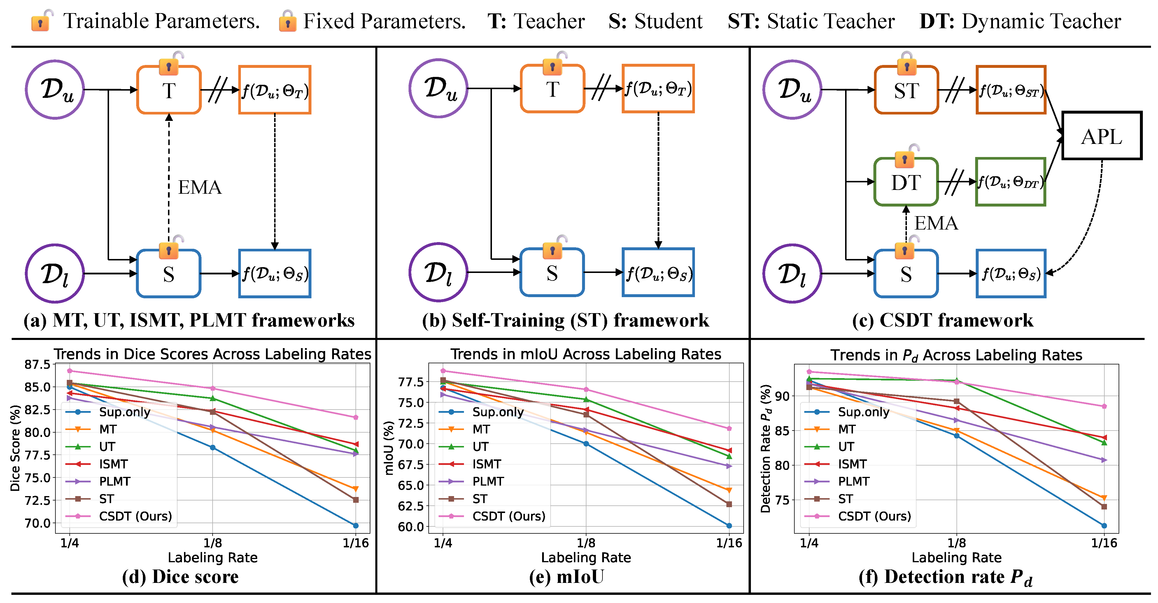
To address these limitations, we propose the novel Multi-Receptive Stripe Attention Network (MRSA-Net), which addresses the challenge of extracting variable and low-SNR stripe targets through multi-receptive field processing and multi-level weighted feature fusion. Additionally, we propose the Collaborative Static-Dynamic Teaching (CSDT) framework, an innovative semi-supervised learning architecture specifically designed for SSTD, as shown in Figure 2c. The CSDT framework leverages the strengths of both labeled and unlabeled data, significantly enhancing detection performance while minimising reliance on labor-intensive manual annotations. The framework employs a dual-teacher setup comprising a static teacher (ST) model, a dynamic teacher (DT) model, and a student (S) model, all configured using the proposed MRSA-Net configuration. The static teacher model is pre-trained on labelled data and remains fixed throughout training, providing consistent guidance. In contrast, the dynamic teacher model is iteratively updated using the exponential moving average (EMA) of the student model’s parameters. This strategy involves blending the student model’s historical parameters from each training cycle to smoothly update the teacher model’s parameters, thereby ensuring it adapts to emerging patterns throughout the training process. Gradient updates are applied exclusively to the student model.
During the training process, the static teacher and dynamic teacher models collaboratively generate pseudo-labels to guide the student model. Initially, the static teacher model offers stable supervision based on its pre-trained knowledge. As training progresses, the framework transitions to adaptive collaborative teaching, where both static teacher and dynamic teacher models contribute pseudo-labels. This transition is orchestrated through a new Adaptive Pseudo-Labeling (APL) strategy, which dynamically selects the most reliable pseudo-labels, adding flexibility and reducing noise in the learning process. This dual-teacher setup enables the student model to progressively adapt to high-quality pseudo-labels, mitigating overfitting risks commonly associated with single-teacher semi-supervised learning methods. During inference, only the dynamic teacher model is utilised, ensuring minimal computational overhead.
As illustrated in Figure 2d–f, we evaluate the SSTD performance of various semi-supervised learning methods on the AstroStripeSet dataset [24] under three labelling rates, with MRSA-Net serving as the teacher-student network. The labeling rate is defined as the ratio of the number of labeled images to the total number of training images. Evaluation metrics include Dice score [25], mean Intersection over Union (mIoU) [26], and detection rate ( P d ) [27]. Results demonstrate the feasibility of semi-supervised learning for SSTD and underscore the significant advantages of the proposed CSDT framework. The compared methods include supervised-only (Sup.only), Mean Teacher (MT) [19], Unbiased Teacher (UT) [20], Interactive Self-Training Mean Teacher (ISMT) [21], Pseudo-Label Mean Teacher (PLMT) [22], and Self-Training (ST) [23]. The primary contributions of this research are outlined below:
  • Novel MRSA-Net: We designed a specialized network for SSTD, which effectively extracts features from variable and low-SNR stripe-like targets using multi-receptive field feature extraction and multi-level weighted feature fusion.
  • Innovative CSDT Architecture: It reduces dependency on extensive, inaccurate, and labor-intensive pixel-level annotations by learning stripe-like patterns from unlabeled space images, marking the first application of semi-supervised learning techniques to SSTD.
  • New Adaptive Pseudo-Labeling (APL) Strategy: It combines insights from static teacher and dynamic teacher models to dynamically select the most reliable pseudo-labels, reducing overfitting risks during training.
  • Comprehensive Validation: Extensive experiments demonstrate the CSDT framework’s state-of-the-art performance on the AstroStripeSet dataset, showcasing robust zero-shot generalization across diverse real-world datasets from both ground-based and space-based sources.
The rest of this paper is is organised into several sections. Section 2 reviews the related work. Section 3 details our CSDT framework for SSTD. Section 4 presents experimental validation results. Section 5 concludes our findings.

2. Related Work

This section reviews the related methods, focusing on traditional unsupervised approaches, fully supervised learning methods, and semi-supervised learning techniques.

2.1. Traditional Unsupervised Methods for SSTD

Traditional unsupervised SSTD methods are broadly categorized into single-frame and multi-frame approaches. Typical single-frame-based methods include Hough [5,10,28,29] and Radon transform [13,30] methods, as well as customized stripe-like pattern filtering methods [14,15,31,32,33]. Hough-based and Radon-based methods utilize traditional median filtering [34] or morphological filtering techniques [35] to eliminate noise and stars, and then employ transform space parameterization to locate stripe-like features. However, these methods are highly sensitive to noise, which prevents distinguishing between background and target signals in low-SNR scenarios, and they are computationally complex. Stripe-like pattern filtering methods design stripe filter templates to match stripe-like targets in the images, but they are limited by the variability of stripe-like targets and heavily dependent on parameter settings. Representative multi-frame methods primarily include time index sequence-based approaches [6,36,37]. These methods use multi-frame information to enhance stripe-like target features and filter out star points, then apply multi-level hypothesis testing to identify stripe-like targets from the remaining candidates. However, They are only applicable to sequential space images with a high SNR. Recently, Lin et al. [9] proposed a method based on stripe-like pattern clustering, but its performance was only reported in slightly noisy scenarios. In summary, traditional unsupervised methods are limited to specific scenarios and exhibit poor generalization in scenarios with variable stripe-like targets, and those with low-SNRs affected by noise such as stray light.

2.2. Fully Supervised Learning Methods for Target Detection

With the rise of CNNs, their application to space images has become a major trend. Jia et al. [16] proposed a framework based on Faster R-CNN for classifying point-like stars and stripe-like space targets, marking the first application of CNN in space scenarios. Li et al. [17] and Liu et al. [18] also developed proprietary CNNs for space stray light removal, demonstrating good performance and further confirming the feasibility of CNNs in space scenarios. Additionally, many fully supervised learning networks have been specifically designed to handle low-SNRs scenarios affected by complex background noise, including UIU-Net [38], DNANet [27], ACM [39], RDIAN [40], ISNet [41], APGCNet [42].
Existing methodological approaches to SSTD provide valuable insights, but they uniformly struggle with detecting variable length and low-SNR stripe-like targets. Most current techniques depend heavily on comprehensive pixel-level annotations, which are labour-intensive and particularly challenging to generate accurately in complex space imaging environments characterised by significant noise interference. Our research introduces a pioneering semi-supervised strategy that directly addresses these methodological constraints, offering a more flexible, accurate and computationally efficient approach to target detection that overcomes the limitations of traditional pixel-level annotation-dependent methods.

2.3. Semi-Supervised Learning Methods for Target Detection

In recent years, to reduce the dependence on extensive data annotation, numerous semi-supervised learning approachs have been proposed across various fields, such as medical segmentation [43,44] and remote sensing [45,46,47,48]. Compared to the fully supervised learning methods, these approaches use a large amount of unlabeled data and a small amount of labeled data to enhance the model’s generalization capabilities.
Current semi-supervised learning approachs fall into two paradigms: consistency regularization-based methods [19,49,50,51] and pseudo-labeling-based methods [20,52,53,54,55]. Consistency regularization, first proposed by Sajjadi et al. [49], ensures that unlabeled data produce consistent outputs under different data augmentations. This approach has been successfully applied to MT [19], temporal ensembling [50], and the cutmix-seg architecture [51], achieving excellent performance. However, these methods assume consistent model outputs for different perturbed inputs, potentially leading to overconfidence in noisy labels and reducing the ability to accurately learn and generalize from the true data structure.
On the other hand, pseudo-labeling methods use labeled data to pre-train the network, then generate labels for unlabeled data through the model itself, and finally incorporate these pseudo-labels into the training process. This approach includes two iterative aspects: (1) the model generates pseudo-labels, and (2) these pseudo-labels are used to update the model weights, leading to the generation of higher-quality pseudo-labels. The advantage of this approach is its ability to dynamically expand the training dataset, but it relies heavily on the quality of the pseudo-labels. Lee et al. [52] first proposed this type of method, and then Sohn et al. [53] added strong image augmentation to enhance the model’s robustness. To address bias and manual intervention in the pseudo-label generation process, Liu et al. [20] and Xu et al. [54] introduced end-to-end strategies based on the MT framework [19]. Specifically, they applyed weak data augmentation in the teacher model and strong data augmentation in the student model to achieve a more robust training process. Moreover, they utilized the EMA mechanism to update the weights of the teacher model, effectively incorporates the historical performance of the student model, smoothing the output of the teacher model. Notably, the EMA mechanism introduced in the MT framework [19] has also been shown in subsequent studies to be crucial for improving semi-supervised learning performance [21,22,55].

3. Proposed Framework

Our proposed framework consists of three key components: First, we introduce MRSA-Net, an innovative network configuration specifically designed for SSTD tasks. It enhances feature extraction for variable and low-SNR stripe-like targets, significantly improving generalization. Next, we present the dual-teacher CSDT semi-supervised learning architecture to address the challenges of inaccurate and labor-intensive manual labeling of stripe-like space targets. Finally, we propose a novel APL strategy to effectively reduce the overfitting risk caused by the rigid teaching methods in existing semi-supervised learning methods.

3.1. MRSA-Net Configuration

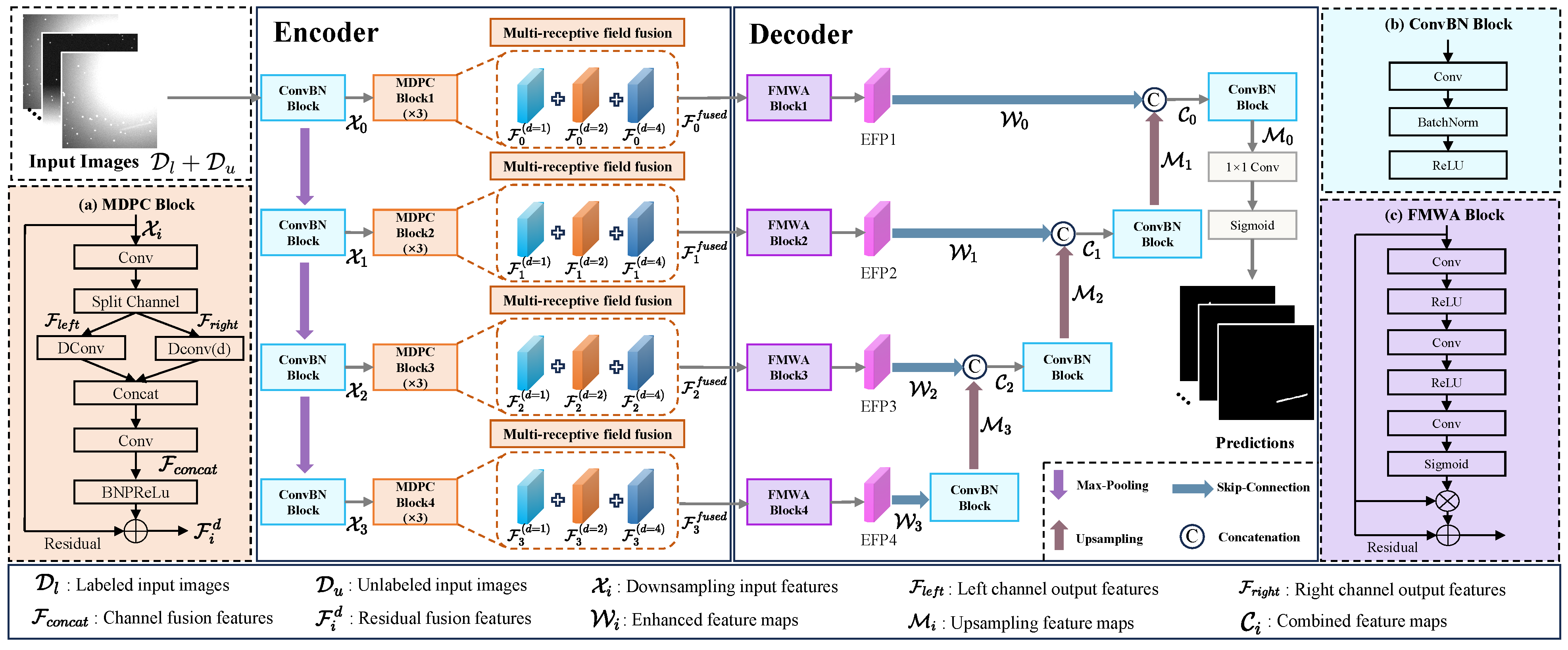
Compared to other fully supervised learning methods [25,56], MRSA-Net improves the network’s ability to extract variable, low-SNR stripe-like targets without a significant increase in parameters. The MRSA-Net is illustrated in Figure 3, consisting of two primary stages: multi-receptive feature extraction endoer and multi-level weighted feature fusion decoder. In the encoder stage, multi-receptive dual-path convolution (MDPC) blocks apply multi-receptive field processing to extract variable length stripe-like features at different levels. In the decoder stage, feature map weighted attention (FMWA) blocks enhance the feature representation of stripe-like target areas, and skip connections dynamically fuse the weighted features from different levels, addressing the issue of feature disappearance in low-SNR stripe-like targets within deep networks.

3.1.1. Multi-Receptive Feature Extraction Encoder

The standard convolution in the existing CNN network [25,27,38,56] performs well for short stripe-like target features but struggles with long-distance stripe-like information due to its limited receptive field. To address this, we designed three MDPC blocks, each with varying dilation rates, strategically placed at each downsampling stage of the encoder. This approach broadens the network’s receptive field, enhancing its adaptability to different spatial resolutions and enabling effective integration of extensive stripe-like feature information. These blocks capture both complex local details and broad contextual information of stripe-like targets. Below are the detailed steps of the MDPC blocks to capture multi-receptive field features.
As shown in Figure 3a, each MDPC block contains two different convolution paths, enhancing the flexibility and efficiency of feature extraction. Initially, the downsampling output features X i undergoes a standard 3 × 3 convolution, producing a feature map while reducing the number of input channels to C / 2 . Subsequently, the feature map is split into two branches, F l e f t and F r i g h t , as follows:
F l e f t = DConv ( Split ( Conv ( X i ) ) ) , F r i g h t = DConv d ( Split ( Conv ( X i ) ) , d ) ,
where X i represents the feature output after the i-th downsampling; Conv ( · ) denotes the standard 3 × 3 convolution; DConv ( · ) refers the depthwise convolution; DConv d ( · ) indicates the depthwise dilated convolution with the specified dilation rate d; and Split ( · ) describes the channel splitting of the feature map.
At this stage, the output channels of the left and right branches are C / 4 each. Specifically, the left path uses depth-wise convolution to precisely capture details of the short stripe-like targets, while the right path employs depth-wise dilated convolution to expand the receptive field and capture broader contextual information. This dual-path design not only enhances the network’s ability to discern the texture information of stripe-like space targets but also improves its capacity to integrate these details over a larger spatial range, thereby significantly enhancing the overall accuracy of the SSTD task. After processing through these two paths, the features are fused and further refined to enhance the stripe saliency of the feature map:
F c o n c a t = Conv ( F l e f t F r i g h t ) ,
where ⊕ represents Concatenation. At this stage, the number of channels of the concatenated feature map ( F l e f t F r i g h t ) is restored to C / 2 . Then, a 3 × 3 convolution restores the number of channels to the original C, while F c o n c a t e extracts more extensive contextual information of the space images than the original input feature X i .
Next, F c o n c a t is batch normalised (BN) and activated via the PReLU function. It is then fused with the downsampling output feature X i through a residual connection to produce the output F i d of each MPDC block. These steps ensure continuity in feature representation and enhance the network’s gradient propagation:
F i d = BNPReLU ( F c o n c a t + X i ) , d { 1 , 2 , 4 } .
Similarly, during each downsampling step, the same procedure is followed to compute the outputs of the three MDPC blocks at varying dilation rates. These outputs are then fused to form a composite feature map F i f u s e d that captures multi-receptive field features. This composite map is subsequently forwarded to the decoder stage, as expressed below:
F i f u s e d = d { 1 , 2 , 4 } F i d , i { 0 , 1 , 2 , 3 } .

3.1.2. Multi-Level Feature Fusion Decoder

In each downsampling step, we also propose a FMWA block to re-represent the feature maps at each level, enhancing the responses of stripe-like pattern regions in F i f u s e d and suppress irrelevant features. Its architecture is shown in Figure 3c, which performs feature transformation through a series of convolution and ReLU layers to enhance the features in a nonlinear manner. A Sigmoid activation layer then generates a weighted attention map, ranging from 0 to 1, to signify the importance of each feature. This weighted attention map is then applied to the input feature map F i f u s e d , dynamically reconstructing important features and amplifying their impact on the final model prediction. Additionally, this block includes residual connections that add the original input F i f u s e d to the weighted output, preserving the integrity of the stripe-like pattern and improving the stability of training. The resulting each enhanced feature map (EFP), denoted as W i , is calculated as follows:
W i = σ ( Conv d e e p ( F i f u s e d ) ) F i f u s e d + F i f u s e d ,
where Conv d e e p represents a deep feature extractor composed of multiple convolutional and ReLU layers; σ ( · ) denotes a Sigmoid function; and ⊙ signifies pixel-level multiplication.
To address the issue of low-SNR stripe-like targets losing features in deep networks, we sequentially feed the enhanced feature maps W i from the FMWA block at each downsampling stage into the ConvBN layers. We then merge up-sampled features M i + 1 with the skip-connected enhanced features W i to reintroduce essential spatial details from early high-resolution layers, producing comprehensive combined feature maps C i . This integration of low-level stripe-like texture information with high-level semantic insights is crucial for restoring textures lost during downsampling. The resulting fused image M 0 , which matches the size of the original image, is subsequently processed by a 1 × 1 convolution and a Sigmoid activation function σ ( · ) to produce accurate predictions of the stripe-like target locations. The approach of this multi-level feature fusion module ensures robust detection capabilities for stripe-like space targets, thus enhancing the reliability in practical applications.

3.2. CSDT Semi-Supervised Learning Architecture

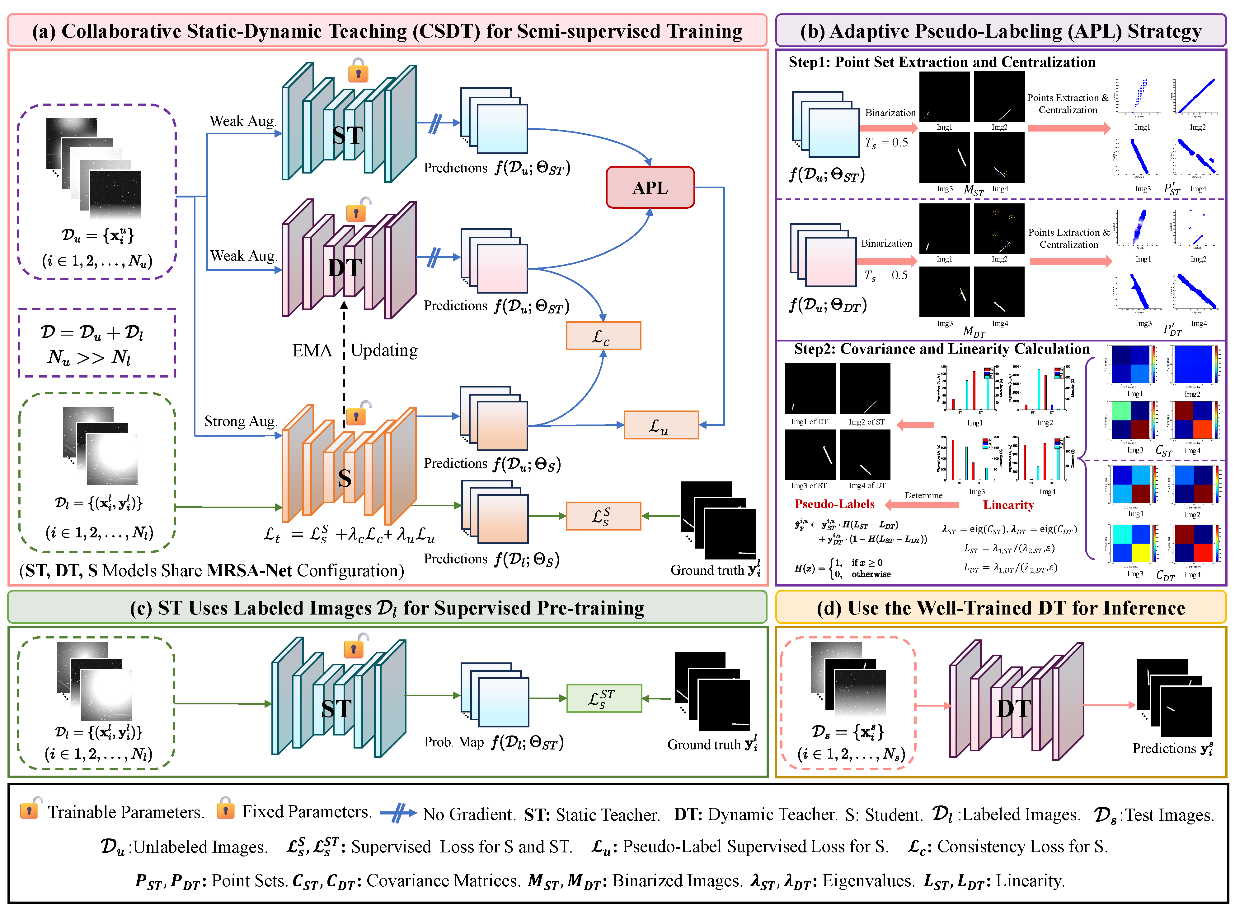
As shown in Figure 4a, our CSDT semi-supervised learning architecture aims to minimize labeling cost for the SSTD task and includes the static teacher model, dynamic teacher model, and student model. All these models share a unified network, MRSA-Net, specifically designed for the SSTD task. During CSDT semi-supervised training, the static teacher and dynamic teacher models employ a novel APL strategy to generate pseudo-labels for unlabeled stripe-like targets, thereby guiding the training of the student model. The weights of the static teacher model remain fixed, while the dynamic teacher model’s weights are updated using the EMA mechanism based on the student model, without gradient updates. Only the student model updates its weights through gradient backpropagation, which encompasses three loss components: supervised loss L s S , pseudo-label supervision loss L u , and consistency loss L c . During inference, only the dynamic teacher model is used to minimize additional time consumption. The detailed CSDT semi-supervised training and updating strategies for these models are outlined in Algorithm 1 and described below.

3.2.1. The Role of the Static Teacher Model

It is initially pre-trained on a limited set of labeled space images D l = { ( x i l , y i l ) | i 1 , 2 , , N l , x i l R H × W × C , y i l R H × W } to provide stable initial guidance for the student model. Here, x i l and y i l represent labeled images and their ground truth (GT), respectively; the parameters H, W, and C denote the height, width, and number of channels of the images, respectively; while N l indicates the number of labeled samples.
To achieve this, samples from D l are iteratively fed into the static teacher model for supervised pre-training using the Dice loss function l d [57], as shown in Figure 4c. The supervised loss for the static teacher model, denoted as L s S T , is calculated as follows:
L s S T = 1 | B l | ( x i l , y i l ) B l l d ( f ( x i l ; Θ S T ) , y i l ) ,
where B l represents a batch of labeled images fed into the static teacher model; Θ S T are the weight parameters of the static teacher model; and the function f ( · ) represents the predictions of the model.
Algorithm 1 CSDT training and updating strategies
Require: 
ST model Θ S T , DT model Θ D T , S model Θ S
Require: 
Labeled images D l = { ( x i l , y i l ) | i { 1 , 2 , , N l } , Unlabeled images D u = { x i u | i { 1 , 2 , , N u }
Require: 
Loss functions L s S T , L s S , L c , L u
Require: 
Loss weight factors λ c , λ u , EMA decay rate α
Require: 
Adaptive pseudo-labeling strategy A P L ( · )
Ensure: 
Well-trained Θ D T ( n u m _ e p o c h s ) for SSTD
1:
Train:
2:
Θ S T , Θ D T , Θ S init ( )                                                                                                     ▹ Initialize all models
3:
t 0                                                                                                                   ▹ Initialize iteration counter
4:
Θ S T train ( x i l , y i l )                                                                                                        ▹ Pre-train ST with D l
5:
for epoch = 1 to num_epochs do
6:
    for each minibatch B l in D l , B u in D u  do
7:
         t t + 1
8:
        for  x i u B u  do
9:
              y S T i , u f ( x i u ; Θ S T )
10:
            y D T i , u f ( x i u ; Θ D T )
11:
            y ^ p i , u A P L ( y S T i , u , y D T i , u )
12:
            L c 1 | B u | l m ( f ( x i u ; Θ S ) , f ( x i u ; Θ D T ) )
13:
            L u 1 | B u | l d ( f ( x i u ; Θ S ) , y ^ p i , u )
14:
        end for
15:
        for  x i l B l  do
16:
            L s S 1 | B l | l d ( f ( x i l ; Θ S ) , y i l )
17:
        end for
18:
         L t L s S + λ c L c + λ u L u                                                                                                         ▹ Update Θ S t
19:
         λ c = exp 5 1 t / t max 2                                                                                         ▹ Ramp-up weight
20:
         Θ D T t α Θ D T t 1 + ( 1 α ) Θ S t                                                                                              ▹ EMA Updating
21:
    end for
22:
end for
23:
Inference:
24:
for each x i s D s  do
25:
       y i s f ( x i s ; Θ D T ( n u m _ e p o c h s ) )                                                                                                  ▹ Predict with Θ D T
26:
end for
As shown in Figure 4a, the static teacher model’s weight parameters are fixed, and only unlabeled images D u = { x i u | i 1 , 2 , , N u , x i u R H × W × C } are fed into it. Serving as a knowledgeable teacher in SSTD, the static teacher model plays a primary teaching role in the early stages of the semi-supervised training process, especially as the dynamic teacher model lacks SSTD capabilities. The main goal of the static teacher model at this stage is to generate pseudo-labels y S T i , u = f ( D u ; Θ S T ) for the unlabeled images D u , providing initial guidance to the student model. This role ensures that the student model starts on the correct learning trajectory, effectively setting a performance baseline within the CSDT framework.

3.2.2. The Role of the Dynamic Teacher Model

Unlike the static teacher model whose weights are fixed, the dynamic teacher model has trainable weights, aiming to offer a more flexible teaching strategy for the student model. We use the EMA mechanism to update its weights, allowing the dynamic teacher model to be dynamically and smoothly adjusted based on the student model’s historical weight parameters. The weight update formula for the dynamic teacher model is as follows:
Θ D T t = α Θ D T t 1 + ( 1 α ) Θ S t ,
where α is the decay rate, typically set between 0.9 and 0.999, to control the influence of the student’s historical information on the dynamic teacher model’s weights. Following the settings of most papers, the value is set to 0.99 in this study. Θ D T and Θ S represent the weight parameters of the dynamic teacher and student models, respectively, and t denotes the current iteration number.
During the CSDT semi-supervised training, the dynamic teacher model is also fed only the unlabeled images D u from the dataset, generating pseudo-labels y D T i , u = f ( D u ; Θ D T ) . During inference, only the dynamic teacher model is used to evaluate on the test dataset D s = { x i s | i 1 , 2 , , N s } , as illustrated in Figure 4d.

3.2.3. The Role of the Student Model

The student model learns from both labeled images D l with ground truth and unlabeled images D u with pseudo-labels provided by the two teacher models, updating its parameters through gradient backpropagation. As training progresses, the teaching mode shifted from the initial fixed guidance of the static teacher model to the adaptive collaborative teaching between the static teacher and dynamic teacher models. This adaptive process involves filtering the optimal pseudo-labels for unlabeled space images from both models, thereby enhancing the overall performance of the student model.
The student model is trained with a customized joint loss function L t , which consists of three components: the supervised loss L s S , the pseudo-label supervised loss L u , and the consistency loss L c . The supervised loss L s S is generated using the labeled images D l and is calculated as follows:
L s S = 1 | B l | ( x i l , y i l ) B l l d ( f ( x i l ; Θ S ) , y i l ) ,
where l d is the Dice loss; B l is a batch of labeled images fed into the student model; and Θ S denotes the weight parameters of the student model.
The consistency loss L c ensures that the student model’s prediction aligns with the dynamic teacher model’s under different augmentation conditions, maintaining uniformity in predictions for unlabeled space images D u . In this paper, we apply colour jittering and Gaussian blur, both at varying intensities, for strong and weak image augmentation, respectively. The consistency loss is calculated as follows:
L c = 1 | B u | x i u B u l m ( f ( x i u ; Θ S ) , f ( x i u ; Θ D T ) ) ,
where B u is a batch of unlabeled images fed into the student model; x i u denotes the unlabeled space images; l m represents the mean squared error (MSE) loss [58].
The pseudo-label supervised loss L u leverages high-quality pseudo-labels provided by either the static teacher model or the dynamic teacher model for learning from unlabeled space images. This loss is specifically designed to uncover deeper insights into the spatial patterns and characteristics of stripe-like targets within the unlabeled space images, thus improving the generalization performance of the student model. It is computed as follows:
L u = 1 | B u | x i u B u l d ( f ( x i u ; Θ S ) , y ^ p i , u ) ,
where l d is the Dice loss, and y ^ p i , u is the optimal pseudo-label generated by either the static teacher model or dynamic teacher model, expressed as y ^ p i , u = A P L ( y S T i , u , y D T i , u ) .
The joint loss L t for the student model is the weighted sum of these individual losses, expressed as follows:
L t = L s + λ c L c + λ u L u ,
where λ u is a fixed constant, and λ c is the ramp-up weight, dynamically adjusting the contribution of the consistency loss L c to the total loss during training, which is defined as:
λ c = exp 5 1 t / t max 2 ,
where exp ( · ) denotes the exponential function; t represents the current iteration number; and t max is the maximum number of iterations.
Initially, L s and L u dominate the loss composition. As training progresses, the weight of L c gradually increases, reflecting its growing importance in fine-tuning the model’s performance. These losses enables the student model to effectively learn from both labeled and unlabeled space images, enhancing its ability to accurately detect stripe-like targets.

3.3. Adaptive Pseudo-Labeling Strategy

The Adaptive Pseudo-Labeling (APL) strategy aims to select the best pseudo-labels from the static teacher and dynamic teacher models to guide the student model’s training. At the beginning of the semi-supervised training, the pseudo-labels generated by the static teacher model are more reliable due to its pre-training. However, the dynamic teacher model’s ability to segment stripe-like targets is quite weak at this stage, resulting in noisy prediction maps. Initially, we use the number of connected components in the prediction map as a straightforward metric to coarsely select the pseudo-labels. As training progresses, the dynamic teacher model gradually improves its performance by leveraging insights into the distribution of unlabeled space images. At this stage, we define a new metric called ‘linearity’ for more refined selection of pseudo labels. The overall process of the proposed APL strategy is detailed as follows:
y ^ p i , u = y S T i , u , if N D T > T c A P L ( y S T i , u , y D T i , u ) . otherwise
Specifically, as illustrated in Figure 4b, we first apply a binarization threshold T s = 0.5 to the Sigmoid predictions of the static teacher and dynamic teacher models to filter out low-confidence predictions, converting them into binary maps M S T = f ( D u ; Θ S T ) > T s and M D T = f ( D u ; Θ D T ) > T s . We then calculate the numbers of connected components N S T and N D T in M S T and M D T , respectively. Next, we define the threshold T c = { max ( N S T i ) | i 1 , 2 , , N u } , based on the maximum number of connected components in all M S T . If N D T > T c , the dynamic teacher model is considered to lack stripe segmentation capability, and the pseudo-labels y S T i , u generated by the static teacher model are directly used to supervise the student model. Conversely, if N D T < T c , the pseudo-labels are selected based on the predictions with higher-quality stripe-like targets from either the static teacher or dynamic teacher models. To facilitate this more refined selection, we define a new ‘linearity’ metric based on the fact that stripe-like targets are typically distributed along a specific direction, as high-quality stripe-like pseudo-labels often exhibit strong linearity. The steps for calculating the ‘linearity’ metric and selecting refined pseudo-labels are as follows:
First, we extract the non-zero pixel regions from the binary images M S T and M D T to form point sets P S T and P D T as follows:
P S T = ( x , y ) R 2 M S T [ x , y ] > 0 , P D T = ( x , y ) R 2 M D T [ x , y ] > 0 .
These two point sets represent the stripe-like target areas predicted by the static teacher and dynamic teacher models, respectively. Next, we calculate the centroid coordinates for each point set using the equations s S T = 1 | P S T | p P S T p and s D T = 1 | P D T | p P D T p , which are denoted by the red symbols ‘’ in Figure 4b. We then perform centralisation preprocessing on each point set to reduce the external differences caused by position deviation and to focus on the internal shape distribution of the stripe-like target. The newly obtained point sets, P S T  and  P D T , are expressed as follows:
P S T = { p s S T p P S T } , P D T = { p s D T p P D T } .
Then, we construct the covariance matrices for the new point sets P S T and P D T as: C S T = 1 | P S T | ( P S T ) T P S T , C D T = 1 | P D T | ( P D T ) T P D T , respectively. The eigenvalues of these covariance matrices are computed as follows:
λ S T = eig ( C S T ) , λ D T = eig ( C D T ) ,
where eig(·) means to obtain the eigenvalue of C S T and C D T . The eigenvalues are arranged in descending order and recorded as λ S T = { λ 1 , S T , λ 2 , S T } and λ D T = { λ 1 , D T , λ 2 , D T } .
Since stripe-like targets exhibit strong directional consistency, a larger λ 1 , * indicates that the model better captures the primary extension direction of stripe-like targets in predicted images. Consequently, diffusion in the width direction should be minimal, requiring λ 2 , to be as small as possible. Based on the meaning of these eigenvalues, we define the ‘linearity’ metric L of each predicted image as follows:
L S T = λ 1 , S T max ( λ 2 , S T , ε ) , L D T = λ 1 , D T max ( λ 2 , D T , ε ) ,
where ε is an infinite decimal to prevent the denominator from being zero, and max(·) represents the maximum function.
From the analysis above, a higher L * value indicates better directionality within the point set, suggesting that the detected stripe-like targets are of higher quality and more appropriate for use as pseudo-labels. Consequently, during training, the CSDT semi-supervised learning framework adaptively identifies the optimal pseudo-labels for unlabeled space images by comparing the linearity metrics  L * of the predictions from the static teacher and dynamic teacher models as follows:
y ^ p i , u = A P L ( y S T i , u , y D T i , u ) = y S T i , u · H ( L S T L D T ) + y D T i , u · ( 1 H ( L S T L D T ) ) ,
where H ( x ) is a step function defined as follows:
H ( x ) = 1 , if x 0 0 . otherwise
In Figure 4b, we display four unlabeled space images (img1 to img4) from a batch to exemplify the proposed APL strategy. This visualisation clearly shows how the APL strategy adaptively selects the optimal quality predictions from the static teacher or dynamic teacher models to serve as the pseudo-labels, denoted y ^ p i , u .

4. Experiments

This section presents a thorough evaluation of the proposed CSDT semi-supervised learning framework. It starts by outlining the experimental setup, including the datasets, evaluation metrics, and implementation details. It then provides a comprehensive analysis through quantitative and visual comparisons with SOTA semi-supervised learning methods across various network configurations. Additionally, the section includes extensive ablation studies to assess the CSDT framework’s generalization capabilities and effectiveness of its key components, such as the zero-shot generalization capabilities of the well-trained models on diverse real-world space image datasets; the effectiveness of MRSA-Net components; the roles of different teacher models in the CSDT; evaluation of the APL strategy; the impact of various loss function combinations; and the comparison with other networks. These experiments collectively underscore the contributions of individual elements to the overall performance of the proposed framework.

4.1. Experimental Setup

This section outlines the experimental setup, starting with an overview of the datasets used in this study, including its composition and the noise challenges it presents. It then discusses the evaluation metrics used to measure model performance at both the pixel and target levels. Finally, it details the implementation, covering hardware and software configurations.

4.1.1. Dataset

We conducted extensive experiments on the AstroStripeSet [24], which contains stripe-like space target images challenged by four types of space stray light noise: earthlight, sunlight, moonlight, and mixedlight. It includes 1000 fixed training images, 100 fixed validation images, and 400 fixed test images, with each stray light noise contributing 100 images to the test set. Notably, nearly all previously published papers have only validated their performance on their in-house datasets, neglecting to use data from other studies to verify the generalization capabilities. To this end, our test dataset incorporated real-world images containing stripe-like space targets that have been used in previous studies [9,17,18]. Since their original images were not publicly available, we used screenshots from published papers to demonstrate our framework’s effectiveness on these datasets. We recognized that screenshots could degrade image quality, but this was the only viable way to obtain these images for our study. To enhance image quality, we applied sharpening filters and contrast adjustments. The dataset also included real-world images with stripe-like space targets collected from the Internet, as well as real-world background images captured by our on-orbit space-based cameras and ground-based telescopes. These diverse sources were used to assess the model’s zero-shot generalization capabilities, testing its effectiveness across a variety of unseen space scenarios.

4.1.2. Evaluation Metrics

We used the Dice coefficient [25] and mIoU [26] metrics to quantitatively evaluate the pixel-level detection performance of the models. These metrics are defined as follows:
mIoU = 1 N i = 1 N y i s y i g t y i s y i g t , Dice = 1 N i = 1 N 2   ×   | y i s y i g t | | y i s | + | y i g t | ,
where y i s and y i g t represent the model predictions and GT of the test images in D s , respectively.
Furthermore, we used widely recognized target detection metrics, including detection rate ( P d ) and false alarm rate ( F a ), to evaluate the target-level performance of the models [27,39,42]. P d measured the probability of correctly detecting targets within a test image subset, where detection was considered successful only if the IoU between the prediction y i s and GT y i g t exceeded 0.5. Meanwhile, F a quantified the proportion of false detections, defined as follows:
P d = N d / N t , F a = N f / N p ,
where N d is the number of correctly detected targets, and N t is the total number of real targets; N f represents the number of falsely detected pixels, while N p denotes the total number of pixels in the test image.

4.1.3. Implementation Details

We train the model using the AstroStripeSet training set. For different label rates γ , the first  1000 γ images are used as labeled data, and the remaining 1000 ( 1 γ ) images are used as unlabeled data for semi-supervised training. All experiments were conducted on a RTX 4080 GPU with 16 GB memory, using PyTorch version 2.2.0 and CUDA version 12.1. During training, we set the batch size B l and B u to 8 for both labeled and unlabeled images, the maximum number of iterations to 25,000, the learning rate to 1 × 10 4 , and used the Adam optimizer for weight updates. The segmentation losses L s and L u utilize the Dice loss, while the consistency loss L c employs the MSE loss. Additionally, the loss weight λ u is fixed at 0.3, and λ c is a ramp-up weight. During inference, only the dynamic teacher model is used for prediction.

4.2. Comparison with SOTA Semi-Supervised Learning Methods

In this section, we evaluated the proposed CSDT framework by comparing it with SOTA semi-supervised learning methods to highlight its advantages. The semi-supervised learning methods compared included MT [19], UT [20], ISMT [21], PLMT [22], and ST [23]. Additionally, we performed comparative experiments with well-known networks such as UCTransNet [25], UNet [56] and our proposed MRSA-Net within these semi-supervised learning methods to highlight MRSA-Net’s superior SSTD performance. Table 1 presents a comparison of the parameter counts and inference times for the three networks. The proposed MRSA-Net not only enhances network performance but also maintains competitive inference speeds comparable to UNet, while requiring significantly fewer parameters than UCTransNet.
Table 2 and Table 3 present the SSTD performance of different SOTA semi-supervised learning methods across three network configurations under noise affected by sunlight, earthlight, moonlight, and mixedlight noise. Performance metrics such as the Dice coefficient, mIoU, and P d are expressed in percentage (%) form, while the F a is presented in an expanded 10 4 format. The top performance metrics are highlighted in bold to signify the best results achieved. We conducted comparative experiments on the AstroStripeSet, utilizing only 1/4, 1/8, and 1/16 of the training set as labeled images, with the remainder being unlabeled images. The label ‘Sup.only’ indicates training only with the labeled images. All evaluated semi-supervised learning methods outperform the ‘Sup.only’ method, improving SSTD performance by learning the distribution of stripe-like targets from unlabeled images, particularly at lower labeling rates. These improvements demonstrate the practicality of the semi-supervised learning approach for SSTD. Our evaluation includes both quantitative comparisons and visual effect assessments.

4.2.1. Quantitative Comparison

Table 2 and Table 3 quantitatively present the average performance on the AstroStripeSet across various labeling rates (1/4, 1/8, 1/16). Our comparative experiments employed UNet, UCTransNet, and our proposed MRSA-Net as segmentation networks. Under these network configurations, our CSDT architecture all achieved notable success. While our CSDT did not achieve the best F a , it excelled in other key performance metrics, surpassing existing SOTA semi-supervised learning methods in the Dice coefficient, mIoU, and P d .
In Table 2, under the UNet configuration with a labeling ratio of 1/4, our CSDT method achieved a Dice coefficient of 83.35%, a mIoU of 75.72%, and a P d of 89.75%. These results represent improvements of 6.28%, 6.90%, and 10.0% over the ‘Sup.only’ method, and also surpass the next best performing ISMT method by 0.08%, 0.86%, and 1.50%, respectively.
When our MRSA-Net operated as the teacher-student network, all semi-supervised learning methods showed greater detection performance improvements than both UNet and UCTransNet configurations. Specifically, with a labeling ratio of 1/8, semi-supervised learning methods, including MT, UT, ISMT, PLMT, ST, and CSDT, showed the following increases in P d : under MRSA-Net, improvements over UNet were 6.50%, 7.50%, 2.25%, 12.75%, 14.50%, and 5.50%, respectively; while improvements over UCTransNet were 5.75%, 1.75%, 1.25%, 5.50%, 10.25%, and 1.25%, respectively. Additionally, at a labeling rate of 1/8, the CSDT method with MRSA-Net even outperformed the CSDT method with UNet at a 1/4 labeling rate. It also matched the performance of the CSDT method with UCTransNet at a 1/4 labeling rate. Similar trends were also observed in the UT and PLMT methods using different networks. These results highlight the clear advantage of MRSA-Net, especially in scenarios with limited labeled images.
Table 3 presents experiments on AstroStripeSet with varying labeling ratios (1/4, 1/8, 1/16) for each type of stray light noise, showing the average detection performance for each category of stray light at these ratios. Our proposed CSDT architecture consistently outperforms other semi-supervised learning methods across three network configurations. Compared to the Sup.only method, all semi-supervised learning methods significant improve in Dice, mIoU, and P d . However, their ability to suppress false alarms has decreased, possibly due to pseudo-label filtering during training of unlabeled images inevitably includes non-target false alarm sources, leading to a higher F a . This limitation highlights a persistent challenge for semi-supervised learning methods. Consequently, based on our APL mechanism, further suppressing false alarm sources in pseudo-labels and adding a rejection strategy to minimize learning of non-target features constitutes the focus of our future research.
To further highlight the advantages of our CSDT framework, we refer to performance indices from the subset tests involving earth light noise. Under MRSA-Net configuration, the CSDT shows improvements of 6.74%, 7.08%, and 8.33% in Dice, mIoU, and P d respectively over the Sup.only method; and 1.93%, 1.96%, and 1.66% improvements over the second-ranked UT method. These improvements are largely attributed to the collaborative efforts of the static and dynamic teachers, along with the novel APL strategy. These settings enable the model to continuously refine the quality of pseudo-labels throughout the training process, fostering a progressive training environment for the student model.
In contrast, the ST method, which utilized a fixed threshold for pseudo-label selection based on model prediction confidence, frequently included poor-quality pseudo-labels in the training process. This inclusion of less accurate labels could limit the model’s overall accuracy. Although the MT method dynamically updated the teacher’s weights via EMA, its feedback strategy was fixed, just focusing on maintaining consistency between the teacher and student predictions. This could lead to the model overfit noisy labels, reducing its ability to deeply understand real stripe-like patterns. Similarly, semi-supervised learning methods like UT, ISMT, and PLMT relied heavily on the pre-trained single-teacher models, leading to rigid teaching approaches that limit the model’s ability to explore new stripe-like pattern distributions. Furthermore, these pre-trained teachers may prematurely adapt to the stripe-like pattern distribution during EMA updates, leading to overfitting and limiting their adaptability in the noisy and variable space scenarios.

4.2.2. Visual Effect Assessments

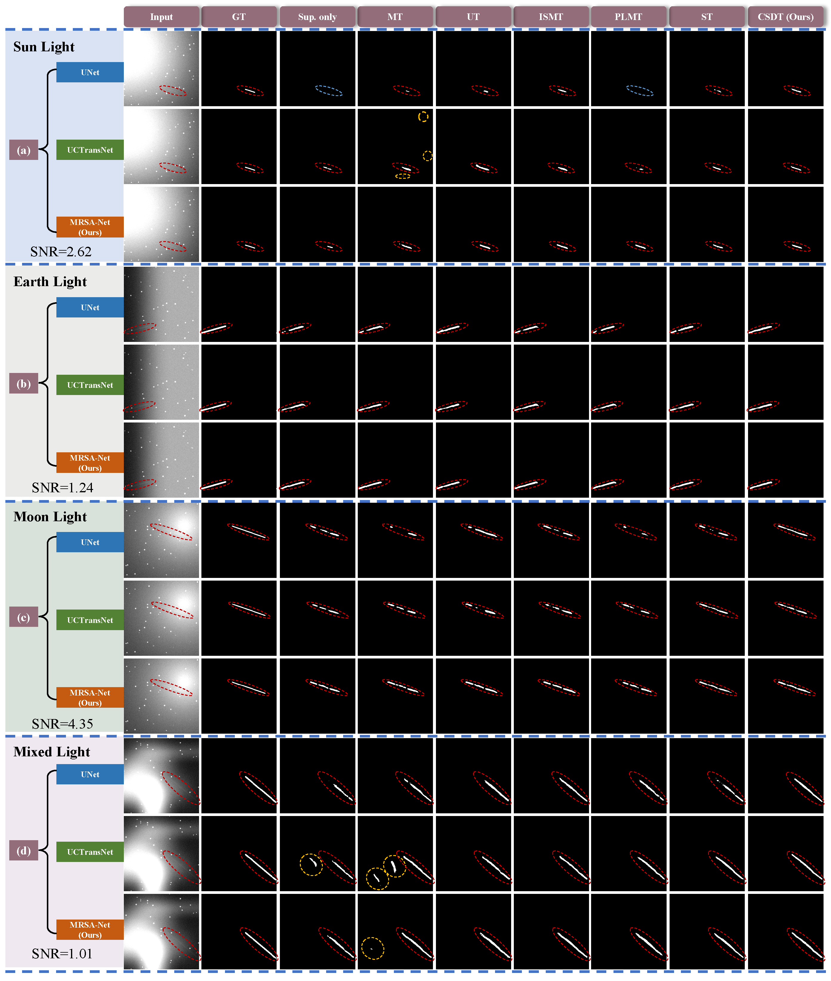
We perform a visual comparison of our method against other semi-supervised learning techniques in low-SNR scenarios, using a 1/4 labeling rate to highlight its distinct advantages. Figure 5 showcases the visual outcomes of different semi-supervised learning methods under three segmentation networks. Figure 5a–d show the detection performance of faint stripe-like space targets under sunlight, earthlight, moonlight, and mixedlight, respectively. Areas of detected real targets are highlighted in the dotted red circle, missed detections are marked in blue, and false alarms are shown in yellow. The proposed CSDT framework significantly enhances SSTD capabilities across all three segmentation networks by preserving target integrity, reducing background noise, and improving overall accuracy and robustness.
Specifically, Figure 5a illustrates that using UNet as the teacher-student network, both the Sup.only and PLMT approachs fail to detect the faint stripe-like target. This detection capability is significantly enhanced by semi-supervised learning methods such as ST, UT, MT, ISMT, and particularly by the proposed CSDT architecture, showcasing the effectiveness of semi-supervised learning methods in the SSTD task. In Figure 5b,c, when using UNet and UCTransNet as the teacher-student networks, almost all compared semi-supervised learning methods show target breakages in their visual results, except the proposed CSDT architecture. This clearly highlights the significant advantage of the dual-teacher adaptive collaborative teaching strategy in our CSDT framework. When MRSA-Net serves as the teacher-student network, it significantly reduces the issue of stripe-like target area breakage in all semi-supervised learning methods, especially within the UT, ISMT, and PLMT methods, leading to notable improvements. These improvements underscore the superiority of MRSA-Net in preserving the integrity of stripe-like targets, even in the scenarios of low-SNR. Moreover, as shown in Figure 5d, when using MRSA-Net as the teacher-student network, each semi-supervised learning method more effectively maintains target integrity compared to UNet. MRSA-Net also more effectively suppresses false alarms than UCTransNet in all semi-supervised learning settings, highlighting its strengths in enhancing stripe-like target continuity and reducing false detections in low-SNR space scenarios. The series of visual comparisons in the Figure 5 highlight the exceptional performance of MRSA-Net in handling low-SNR targets across various scenarios. These comparisons also demonstrate that the CSDT framework effectively extracts new knowledge from unlabeled space images, thereby improving the model’s generalization performance.

4.3. Ablation Study

In this section, we assess the effectiveness of various modules within our proposed framework through detailed experiments, commonly referred to as ablation studies. We assessed the CSDT framework’s generalization capabilities with real-world datasets in zero-shot settings; the contributions of each MRSA-Net component; the role of dual teachers; the impact of the APL strategy; the role of each loss function; and the comparison with other networks.

4.3.1. Zero-Shot Generalization Capabilities

In this section, we have specifically designed experiments to assess the performance of each model on real-world datasets that were not included in the training process. These are referred to as zero-shot generalization validation experiments. To the best of our knowledge, this aspect is often overlooked in most papers within the SSTD field. Figure 6 displays the zero-shot generalization results of different semi-supervised learning methods on real-world image datasets using MRSA-Net as the teacher-student network at a labeling rate of 1/16. Figure 6a features data from [9]; Figure 6b uses data from [17]; Figure 6c incorporates data from [18]; and Figure 6d includes data collected from the Internet; Figure 6e,f and Figure 6g,h show real-space background images taken by our on-orbit space-based camera and ground-based telescope, respectively. These figures reveal significant differences in zero-shot generalization performance among the semi-supervised learning methods.
As demonstrated in Table 4, the CSDT framework delivers the best detection results overall, except for img(c), where UT and PLMT methods perform slightly better. This discrepancy is due to the APL strategy incorporating many high-quality stripe-like pseudo-labels, which enhances stripe-like pattern segmentation but might also lead to some false alarms in the presence of stripe-like noise. For other semi-supervised learning methods, stripe-like targets are detected in simpler background scenarios (Figure 6a,b). However, false detections (yellow marks, Figure 6c,f,g) and missed detections (blue marks, Figure 6d) occurred in more challenging cases. Additionally, in Figure 6e, semi-supervised learning methods like ST, MT, and PLMT exhibit significant breakage in the stripe-like target areas, and UT and ISMT also result in more false alarms than the proposed CSDT method. These outcomes highlight the limitations of these rigid teaching models, which cannot dynamically adapt their strategies to improve pseudo-label quality, thus restricting improvements in generalization capabilities to unknown data. Thus, we not only validate the effectiveness of our proposed method in a standard test environment but also demonstrate its reliability in real-world applications.

4.3.2. Contribution of MRSA-Net Components

In this section, we evaluated the effectiveness of the MDPC and FMWA blocks, two critical components proposed in MRSA-Net. We utilized 1/4 of the labeled space images from AstroStripeSet for Sup.only training, and evaluate the contribution of each block. As detailed in Table 5, the Baseline achieved the lowest F a compared to MRSA-Net. This is because the MDPC and FMWA blocks, while enhancing weakly textured stripe-like target feature extraction, also capture some stray light regions similar to stripe-like targets, leading to a slight increase in F a . When the baseline is equipped with MDPC blocks, mIoU and P d increase by 6.77% and 10.75%, respectively, indicating that multi-receptive field processing enhances the feature extraction of variable stripe targets. With FMWA blocks, mIoU and P d improve by 3.27% and 4.50%, respectively, showing that the FMWA block boosts sensitivity to low-SNR stripe-like targets through feature reconstruction. Our MRSA-Net, which incorporates both MDPC and FMWA blocks, achieves a 7.94% and 12.50% increase in mIoU and P d , respectively, demonstrating that the combination of multi-receptive field extraction and multi-level feature reconstruction effectively addresses the challenges of variable stripe-like targets detection and low-SNR feature disappearance.
Furthermore, we conducted an ablation study to determine the optimal number of MDPC blocks. Table 6 reveal that the best detection performance is achieved with three MDPC blocks. This finding indicates that three MDPC blocks strike an optimal balance between coverage and specificity, preserving pixel-level details of stripe-like targets while enhancing detection accuracy at the target-level. This balance is crucial in complex space scenarios, where too few blocks might miss finer stripe-like target details and too many could lead to overfitting on noise.

4.3.3. Single-Teacher vs. Dual-Teacher Supervision

Table 7 displays the SSTD performance at a labeling rate of 1/16 across various configurations: using both teachers (static teacher and dynamic teacher together), one teacher (static teacher or dynamic teacher alone), and no teacher (Sup.only). With only the static teacher model, the semi-supervised learning framework utilizes pseudo-label segmentation loss L u for unlabeled images, without involving EMA. With only the dynamic teacher model, it depends on consistency loss L c to use unlabeled images, aiming to maintain output consistency between dynamic teacher and the student model. Table 7 shows that our CSDT framework, which integrates both the static teacher and dynamic teacher models, significantly outperforms other setups. This enhanced performance is attributed to the fusion of the strengths of the static teacher and dynamic teacher models, as well as the application of the APL strategy. It adaptively employs high-quality pseudo-labels, which not only enhances the student model’s performance but also continuously improves dynamic teacher’s performance through the EMA mechanism, thereby further refining the pseudo-label quality and creating a positive feedback loop. This strategy efficiently utilizes unlabeled images and minimizes the impact of incorrect labels, thus boosting overall accuracy and model generalization across diverse space scenarios. Ablation study results further confirm that CSDT architecture is highly effective for the SSTD task.

4.3.4. Evaluation of APL Strategy

Within the CSDT framework, we assessed the average SSTD performance using different pseudo-labeling (PL) strategies at a labeling rate of 1/16. Since the static teacher model is pre-trained, it initially outperforms the dynamic teacher model. However, dynamic teacher’s performance enhances as it progressively learns from the student model. Therefore, it is obvious that we can directly use the prediction of the static teacher model for the initial N epochs and switch to dynamic teacher’s predictions thereafter. We denote this method as the ST → DT PL strategy. Additionally, using either the intersection (ST ∩ DT) or the union (ST ∪ DT) of the predictions from static teacher and dynamic teacher as pseudo-labels represent two other intuitive PL strategies. To demonstrate the superiority of our APL strategy, we compared it against these more straightforward PL approaches that lack adaptive selection mechanisms. As illustrated in Table 8, the APL strategy significantly outperforms the fixed PL strategies across all metrics. This is because the APL strategy cleverly utilizes the prior knowledge of directional consistency inherent in the stripe-like space targets during the pseudo-labeling process. Based on this, we introduce a novel metric of ‘linearity’ enabling the adaptive selection of optimal pseudo-labels from the static teacher and dynamic teacher models, thereby better teaching the student model during training.

4.3.5. Impact of Loss Functions

Within the CSDT framework, we conducted a loss function ablation study using MRSA-Net as the teacher-student network at a 1/16 labeling rate. We explored three different loss functions for the student model: supervised loss L s S for labeled images, pseudo-label supervised loss L u for unlabeled images, and consistency loss L c for maintaining output consistency between the student model and dynamic teacher model across different augmentations of unlabeled images. Table 9 shows the impact of these losses on the average performance under four types of stray light noise of AstroStripeSet.
Table 9 shows that using L s S , L u , and L c together yields the best performance in Dice, mIoU, P d , and F a metrics, with specific values of 81.63%, 71.84%, 88.50%, and 5.75% respectively. This confirms that integrating these three loss functions significantly enhances the accuracy of SSTD. Upon removing L c , a noticeable decline in performance occurs, with Dice and mIoU values decreasing to 80.55% and 70.84%, respectively. This underscores the vital role of consistency loss L c in utilizing unlabeled images for training. The subsequent removal of L u leads to a more pronounced performance drop, with Dice and mIoU plummeting to 76.59% and 67.16%. This illustrates the critical importance of pseudo-label loss L u in enhancing the model’s generalization capabilities and minimizing overfitting. Relying solely on L s S results in the lowest performance, with Dice and mIoU at 69.69% and 60.09%, respectively. Therefore, the pseudo-label supervised loss L u is crucial for harnessing the latent information in unlabeled images, enabling the model to adapt to the intrinsic data variability and improve robustness. Consistency loss L c ensures that the model’s predictions are stable across different augmentations of the same input, which is vital for maintaining reliable predictions in diverse and complex space imaging scenarios.

4.3.6. Comparison with Other Networks

To further demonstrate the outstanding performance of the proposed MRSA-Net, we compare it with several advanced network architectures using Sup.only training at a 1/4 label rate. Given the absence of networks specifically tailored for stripe-like space target detection, the benchmarks include classic models such as UNet and UCTransNet, as well as SOTA networks like MSHNet and RDIAN, which are designed for detecting infrared weak targets. As shown in Table 10, MRSA-Net outperforms the others across key metrics such as Dice, mIoU, and P d . While MSHNet [59] and RDIAN [39] are effective for sparse point target detection, their structures are primarily optimized for small targets and struggle to model the long-distance spatial dependencies characteristic of stripe-like targets. This result emphatically confirms the effectiveness of MRSA-Net’s architecture for handling stripe-like targets.

5. Conclusions

This paper introduces the Collaborative Static-Dynamic Teaching (CSDT) framework, a novel semi-supervised learning approach tailored for stripe-like space target detection (SSTD). By leveraging labelled and unlabeled data, the CSDT framework enhances detection performance under low signal-to-noise ratio (SNR) conditions while reducing the reliance on manual annotations. Its dual-teacher setup, comprising static and dynamic teacher models, alongside the MRSA-Net architecture and adaptive pseudo-labeling (APL) strategy, ensures robust generalisation and high-quality pseudo-label generation. Extensive experiments on the AstroStripeSet and other real-world datasets demonstrate the framework’s superior performance in key metrics, including Dice score, mean Intersection over Union (mIoU), and detection rate ( P d ). Additionally, its robust zero-shot generalisation highlights practical applicability across diverse scenarios. Future work will focus on expanding to related domains, incorporating transfer learning, and addressing real-time performance challenges to improve the framework’s scalability and impact.

Author Contributions

Conceptualization, Z.Z.; methodology, Z.Z.; software, Z.Z.; validation, Z.Z., A.Z., X.L. and B.D.; investigation, Z.Z. and Y.M.; resources, R.Z. and E.L.; writing—original draft, Z.Z.; writing-review and editing, Z.Z., A.Z., and B.D.; visualization, Z.Z., B.D., K.L. and H.L.; supervision, E.L. and R.Z.; project administration, R.Z.; funding acquisition, R.Z. All authors have read and agreed to the published version of the manuscript.

Funding

This work was supported in part by China Scholarship Council No. 202304910543, the Sichuan Outstanding Youth Science and Technology Talent Project No. 2022JDJQ0027, and the Department of Science and Technology of Sichuan Province No. 2022JDRC0065 and No. 2024NSFSC1443.

Data Availability Statement

The data and code are available at https://github.com/BenZae/CSDT_SSL/tree/master (accessed on 22 December 2024).

Acknowledgments

Thanks to the collaborators in the Department of the Institute of Optics and Electronics, Chinese Academy of Sciences, and the Australian National University.

Conflicts of Interest

The authors declare no conflict of interest.

References

  1. Li, Z.; Wang, Y.; Zheng, W. Space-based optical observations on space debris via multipoint of view. Int. J. Aerosp. Eng. 2020, 2020, 8328405. [Google Scholar] [CrossRef]
  2. Wirnsberger, H.; Baur, O.; Kirchner, G. Space debris orbit prediction errors using bi-static laser observations. Case study: ENVISAT. Adv. Space Res. 2015, 55, 2607–2615. [Google Scholar] [CrossRef]
  3. Zhang, J.; Shi, A.; Yang, K. Dynamics of tethered-coulomb formation for debris deorbiting in geosynchronous orbit. J. Aerosp. Eng. 2022, 35, 04022015. [Google Scholar] [CrossRef]
  4. Liu, D.; Chen, B.; Chin, T.J.; Rutten, M.G. Topological sweep for multi-target detection of geostationary space objects. IEEE Trans. Signal Process. 2020, 68, 5166–5177. [Google Scholar] [CrossRef]
  5. Diprima, F.; Santoni, F.; Piergentili, F.; Fortunato, V.; Abbattista, C.; Amoruso, L. Efficient and automatic image reduction framework for space debris detection based on GPU technology. Acta Astronaut. 2018, 145, 332–341. [Google Scholar] [CrossRef]
  6. Liu, D.; Wang, X.; Xu, Z.; Li, Y.; Liu, W. Space target extraction and detection for wide-field surveillance. Astron. Comput. 2020, 32, 100408. [Google Scholar] [CrossRef]
  7. Yao, Y.; Zhu, J.; Liu, Q.; Lu, Y.; Xu, X. An adaptive space target detection algorithm. IEEE Geosci. Remote Sens. Lett. 2022, 19, 6517605. [Google Scholar] [CrossRef]
  8. Felt, V.; Fletcher, J. Seeing Stars: Learned Star Localization for Narrow-Field Astrometry. In Proceedings of the IEEE/CVF Winter Conference on Applications of Computer Vision, Nashville TN, USA, 11–15 June 2024; pp. 8297–8305. [Google Scholar]
  9. Lin, B.; Zhong, L.; Zhuge, S.; Yang, X.; Yang, Y.; Wang, K.; Zhang, X. A New Pattern for Detection of Streak-like Space Target From Single Optical Images. IEEE Trans. Geosci. Remote Sens. 2021, 60, 5616113. [Google Scholar] [CrossRef]
  10. Jiang, P.; Liu, C.; Yang, W.; Kang, Z.; Li, Z. Automatic space debris extraction channel based on large field of view photoelectric detection system. Publ. Astron. Soc. Pac. 2022, 134, 024503. [Google Scholar] [CrossRef]
  11. Lu, K.; Li, H.; Lin, L.; Zhao, R.; Liu, E.; Zhao, R. A Fast Star-Detection Algorithm under Stray-Light Interference. Photonics 2023, 10, 889. [Google Scholar] [CrossRef]
  12. Xu, Z.; Liu, D.; Yan, C.; Hu, C. Stray light nonuniform background correction for a wide-field surveillance system. Appl. Opt. 2020, 59, 10719–10728. [Google Scholar] [CrossRef] [PubMed]
  13. Hickson, P. A fast algorithm for the detection of faint orbital debris tracks in optical images. Adv. Space Res. 2018, 62, 3078–3085. [Google Scholar] [CrossRef]
  14. Levesque, M.P.; Buteau, S. Image Processing Technique for Automatic Detection of Satellite Streaks; Defense Research and Development Canada Valcartier: Quebec, QC, Canada, 2007. [Google Scholar]
  15. Levesque, M. Automatic reacquisition of satellite positions by detecting their expected streaks in astronomical images. In Proceedings of the Advanced Maui Optical and Space Surveillance Technologies Conference, Wailea, HI, USA, 19–22 September 2009; p. E81. [Google Scholar]
  16. Jia, P.; Liu, Q.; Sun, Y. Detection and classification of astronomical targets with deep neural networks in wide-field small aperture telescopes. Astron. J. 2020, 159, 212. [Google Scholar] [CrossRef]
  17. Li, Y.; Niu, Z.; Sun, Q.; Xiao, H.; Li, H. BSC-Net: Background Suppression Algorithm for Stray Lights in Star Images. Remote Sens. 2022, 14, 4852. [Google Scholar] [CrossRef]
  18. Liu, L.; Niu, Z.; Li, Y.; Sun, Q. Multi-Level Convolutional Network for Ground-Based Star Image Enhancement. Remote Sens. 2023, 15, 3292. [Google Scholar] [CrossRef]
  19. Tarvainen, A.; Valpola, H. Mean teachers are better role models: Weight-averaged consistency targets improve semi-supervised deep learning results. Adv. Neural Inf. Process. Syst. 2017, 30, 789. [Google Scholar]
  20. Liu, Y.C.; Ma, C.Y.; He, Z.; Kuo, C.W.; Chen, K.; Zhang, P.; Wu, B.; Kira, Z.; Vajda, P. Unbiased teacher for semi-supervised object detection. arXiv 2021, arXiv:2102.09480. [Google Scholar]
  21. Yang, Q.; Wei, X.; Wang, B.; Hua, X.S.; Zhang, L. Interactive self-training with mean teachers for semi-supervised object detection. In Proceedings of the IEEE/CVF Conference on Computer Vision and Pattern Recognition, Nashville, TN, USA, 20–25 June 2021; pp. 5941–5950. [Google Scholar]
  22. Mao, Z.; Tong, X.; Luo, Z. Semi-Supervised Remote Sensing Image Change Detection Using Mean Teacher Model for Constructing Pseudo-Labels. In Proceedings of the ICASSP 2023—2023 IEEE International Conference on Acoustics, Speech and Signal Processing (ICASSP), Rhodes Island, Greece, 4–10 June 2023; pp. 1–5. [Google Scholar]
  23. Yang, L.; Zhuo, W.; Qi, L.; Shi, Y.; Gao, Y. St++: Make self-training work better for semi-supervised semantic segmentation. In Proceedings of the IEEE/CVF Conference on Computer Vision and Pattern Recognition, New Orleans, LA, USA, 18–24 June 2022; pp. 4268–4277. [Google Scholar]
  24. Zhu, Z.; Zia, A.; Li, X.; Dan, B.; Ma, Y.; Liu, E.; Zhao, R. SSTD: Stripe-Like Space Target Detection using Single-Point Supervision. arXiv 2024, arXiv:2407.18097. [Google Scholar]
  25. Wang, H.; Cao, P.; Wang, J.; Zaiane, O.R. Uctransnet: Rethinking the skip connections in u-net from a channel-wise perspective with transformer. In Proceedings of the AAAI Conference on Artificial Intelligence, Online, 22 February–1 March 2022; Volume 36, pp. 2441–2449. [Google Scholar]
  26. Ma, T.; Wang, H.; Liang, J.; Peng, J.; Ma, Q.; Kai, Z. MSMA-Net: An Infrared Small Target Detection Network by Multi-scale Super-resolution Enhancement and Multi-level Attention Fusion. IEEE Trans. Geosci. Remote. Sens. 2023, 62, 5602620. [Google Scholar]
  27. Li, B.; Xiao, C.; Wang, L.; Wang, Y.; Lin, Z.; Li, M.; An, W.; Guo, Y. Dense nested attention network for infrared small target detection. IEEE Trans. Image Process. 2022, 32, 1745–1758. [Google Scholar] [CrossRef]
  28. Jiang, P.; Liu, C.; Yang, W.; Kang, Z.; Fan, C.; Li, Z. Space Debris Automation Detection and Extraction Based on a Wide-field Surveillance System. Astrophys. J. Suppl. Ser. 2022, 259, 4. [Google Scholar] [CrossRef]
  29. Cegarra Polo, M.; Yanagisawa, T.; Kurosaki, H. Real-time processing pipeline for automatic streak detection in astronomical images implemented in a multi-GPU system. Publ. Astron. Soc. Jpn. 2022, 74, 777–790. [Google Scholar] [CrossRef]
  30. Nir, G.; Zackay, B.; Ofek, E.O. Optimal and efficient streak detection in astronomical images. Astron. J. 2018, 156, 229. [Google Scholar] [CrossRef]
  31. Dawson, W.A.; Schneider, M.D.; Kamath, C. Blind detection of ultra-faint streaks with a maximum likelihood method. arXiv 2016, arXiv:1609.07158. [Google Scholar]
  32. Sara, R.; Cvrcek, V. Faint streak detection with certificate by adaptive multi-level bayesian inference. In Proceedings of the European Conference on Space Debris, Darmstadt, Germany, 18–21 April 2017. [Google Scholar]
  33. Virtanen, J.; Poikonen, J.; Säntti, T.; Komulainen, T.; Torppa, J.; Granvik, M.; Muinonen, K.; Pentikäinen, H.; Martikainen, J.; Näränen, J.; et al. Streak detection and analysis pipeline for space-debris optical images. Adv. Space Res. 2016, 57, 1607–1623. [Google Scholar] [CrossRef]
  34. Huang, T.; Yang, G.; Tang, G. A fast two-dimensional median filtering algorithm. IEEE Trans. Acoust. Speech Signal Process. 1979, 27, 13–18. [Google Scholar] [CrossRef]
  35. Serra, J.; Vincent, L. An overview of morphological filtering. Circuits Syst. Signal Process. 1992, 11, 47–108. [Google Scholar] [CrossRef]
  36. Xi, J.; Wen, D.; Ersoy, O.K.; Yi, H.; Yao, D.; Song, Z.; Xi, S. Space debris detection in optical image sequences. Appl. Opt. 2016, 55, 7929–7940. [Google Scholar] [CrossRef]
  37. Duarte, P.; Gordo, P.; Peixinho, N.; Melicio, R.; Valério, D.; Gafeira, R. Space Surveillance payload camera breadboard: Star tracking and debris detection algorithms. Adv. Space Res. 2023, 72, 4215–4228. [Google Scholar]
  38. Wu, X.; Hong, D.; Chanussot, J. UIU-Net: U-Net in U-Net for infrared small object detection. IEEE Trans. Image Process. 2022, 32, 364–376. [Google Scholar] [CrossRef]
  39. Dai, Y.; Wu, Y.; Zhou, F.; Barnard, K. Asymmetric contextual modulation for infrared small target detection. In Proceedings of the IEEE/CVF Winter Conference on Applications of Computer Vision, Virtual, 5–9 January 2021; pp. 950–959. [Google Scholar]
  40. Sun, H.; Bai, J.; Yang, F.; Bai, X. Receptive-Field and Direction Induced Attention Network for Infrared Dim Small Target Detection with a Large-Scale Dataset IRDST. IEEE Trans. Geosci. Remote Sens. 2023, 61, 5000513. [Google Scholar] [CrossRef]
  41. Zhang, M.; Zhang, R.; Yang, Y.; Bai, H.; Zhang, J.; Guo, J. ISNet: Shape matters for infrared small target detection. In Proceedings of the IEEE/CVF Conference on Computer Vision and Pattern Recognition, New Orleans, LA, USA, 18–24 June 2022; pp. 877–886. [Google Scholar]
  42. Zhang, T.; Cao, S.; Pu, T.; Peng, Z. AGPCNet: Attention-guided pyramid context networks for infrared small target detection. arXiv 2021, arXiv:2111.03580. [Google Scholar]
  43. Cao, K.; Liu, Y.; Zeng, X.; Qin, X.; Wu, R.; Wan, L.; Deng, B.; Zhong, J.; Ni, G.; Liu, Y. Semi-supervised 3D retinal fluid segmentation via correlation mutual learning with global reasoning attention. Biomed. Opt. Express 2024, 15, 6905–6921. [Google Scholar] [CrossRef]
  44. Hu, S.; Tang, H.; Luo, Y. Identifying retinopathy in optical coherence tomography images with less labeled data via contrastive graph regularization. Biomed. Opt. Express 2024, 15, 4980–4994. [Google Scholar] [CrossRef]
  45. Chen, H.; Li, Z.; Wu, J.; Xiong, W.; Du, C. SemiRoadExNet: A semi-supervised network for road extraction from remote sensing imagery via adversarial learning. ISPRS J. Photogramm. Remote Sens. 2023, 198, 169–183. [Google Scholar] [CrossRef]
  46. Sun, B.; Zhang, Y.; Zhou, Q.; Zhang, X. Effectiveness of semi-supervised learning and multi-source data in detailed urban landuse mapping with a few labeled samples. Remote Sens. 2022, 14, 648. [Google Scholar] [CrossRef]
  47. Chen, Z.; Wang, R.; Xu, Y. Semi-Supervised Remote Sensing Building Change Detection with Joint Perturbation and Feature Complementation. Remote Sens. 2024, 16, 3424. [Google Scholar] [CrossRef]
  48. Yang, Y.; Lang, P.; Yin, J.; He, Y.; Yang, J. Data Matters: Rethinking the Data Distribution in Semi-Supervised Oriented SAR Ship Detection. Remote Sens. 2024, 16, 2551. [Google Scholar] [CrossRef]
  49. Sajjadi, M.; Javanmardi, M.; Tasdizen, T. Regularization with stochastic transformations and perturbations for deep semi-supervised learning. Adv. Neural Inf. Process. Syst. 2016, 29. [Google Scholar]
  50. Laine, S.; Aila, T. Temporal ensembling for semi-supervised learning. arXiv 2016, arXiv:1610.02242. [Google Scholar]
  51. Sohn, K.; Berthelot, D.; Carlini, N.; Zhang, Z.; Zhang, H.; Raffel, C.A.; Cubuk, E.D.; Kurakin, A.; Li, C.L. Fixmatch: Simplifying semi-supervised learning with consistency and confidence. Adv. Neural Inf. Process. Syst. 2020, 33, 596–608. [Google Scholar]
  52. Lee, D.H. Pseudo-label: The simple and efficient semi-supervised learning method for deep neural networks. In Proceedings of the Workshop on Challenges in Representation Learning, ICML, Atlanta, GA, USA, 17–19 June 2013; Volume 3, p. 896. [Google Scholar]
  53. Sohn, K.; Zhang, Z.; Li, C.L.; Zhang, H.; Lee, C.Y.; Pfister, T. A simple semi-supervised learning framework for object detection. arXiv 2020, arXiv:2005.04757. [Google Scholar]
  54. Xu, M.; Zhang, Z.; Hu, H.; Wang, J.; Wang, L.; Wei, F.; Bai, X.; Liu, Z. End-to-end semi-supervised object detection with soft teacher. In Proceedings of the IEEE/CVF International Conference on Computer Vision, Montreal, QC, Canada, 10–17 October 2021; pp. 3060–3069. [Google Scholar]
  55. Zhou, Y.; Jiang, X.; Chen, Z.; Chen, L.; Liu, X. A Semi-Supervised Arbitrary-Oriented SAR Ship Detection Network based on Interference Consistency Learning and Pseudo Label Calibration. IEEE J. Sel. Top. Appl. Earth Obs. Remote. Sens. 2023, 16, 5893–5904. [Google Scholar] [CrossRef]
  56. Ronneberger, O.; Fischer, P.; Brox, T. U-net: Convolutional networks for biomedical image segmentation. In Medical Image Computing and Computer-Assisted Intervention—MICCAI 2015, Proceedings of the 18th International Conference, Munich, Germany, 5–9 October 2015; proceedings, part III 18; Springer: Berlin/Heidelberg, Germany, 2015; pp. 234–241. [Google Scholar]
  57. Mei, C.; Yang, X.; Zhou, M.; Zhang, S.; Chen, H.; Yang, X.; Wang, L. Semi-supervised image segmentation using a residual-driven mean teacher and an exponential Dice loss. Artif. Intell. Med. 2024, 148, 102757. [Google Scholar] [CrossRef]
  58. Yang, X.; Song, Z.; King, I.; Xu, Z. A survey on deep semi-supervised learning. IEEE Trans. Knowl. Data Eng. 2022, 35, 8934–8954. [Google Scholar] [CrossRef]
  59. Liu, Q.; Liu, R.; Zheng, B.; Wang, H.; Fu, Y. Infrared small target detection with scale and location sensitivity. In Proceedings of the IEEE/CVF Conference on Computer Vision and Pattern Recognition, Seattle, WA, USA, 16–22 June 2024; pp. 17490–17499. [Google Scholar]
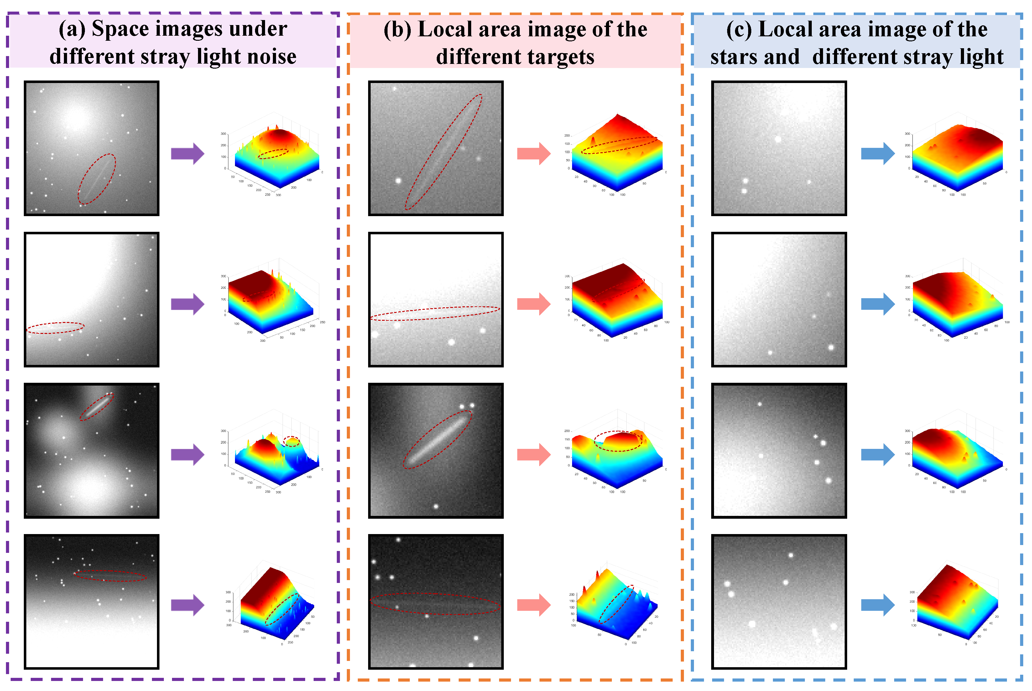
Figure 1. Representative space images with low signal-to-noise ratio stripe-like targets (The red dotted circle represents the stripe-like targets).
Remotesensing 17 01341 g001
Figure 2. Comparison of semi-supervised learning architectures with MRSA-Net as the teacher-student network: (a) Single-teacher architectures based on exponential moving average (EMA) strategies, including Mean Teacher (MT) [19], Unbiased Teacher (UT) [20], Interactive Self-Training Mean Teacher (ISMT) [21], and Pseudo-Label Mean Teacher (PLMT) [22]. (b) Self-Training (ST) [23], a single-teacher architecture without EMA. (c) Our proposed Collaborative Static-Dynamic Teaching (CSDT) architecture utilizing EMA. Panels (df) show the performances of these semi-supervised learning architectures in terms of Dice score, mIoU, and detection rate P d across various labeling rates.
Remotesensing 17 01341 g002
Figure 3. Overall configuration of MRSA-Net comprises two main parts: the encoder and the decoder. (a) The proposed MDPC block, designed to expand the receptive field and extract multi-receptive stripe-like features. (b) The internal architecture of the ConvBN block. (c) The proposed FMWA block, which enhances the stripe-like target regions in the feature map through feature reconstruction and suppresses noise.
Remotesensing 17 01341 g003
Figure 4. Overview of our proposed CSDT semi-supervised learning framework. (a) CSDT uses both labeled images D l and unlabeled images D u for semi-supervised training. (b) Details of the APL strategy implementation, which involves point set extraction and centralization, followed by covariance and linearity calculations. (c) static teacher uses a small subset of labeled images D l for pre-training. (d) During inference, only the well-trained dynamic teacher is utilized.
Remotesensing 17 01341 g004
Figure 5. Visualization results of different semi-supervised learning methods on AstroStripeSet using three network configurations: UNet, UCTransNet, and MRSA-Net as segmentation networks. Evaluations are conducted across these networks at a labeling rate of 1/4 (Detected real stripe-like targets are highlighted in the dotted red circle, missed detections are marked in blue, and false alarms are presented in yellow).
Remotesensing 17 01341 g005
Figure 6. Visualization of the SSTD results using various semi-supervised learning methods on real-world datasets with MRSA-Net as the teacher-student network at a 1/16 labeling rate (Detected real stripe-like targets are highlighted in the dotted red circle, missed detections are marked in blue, and false alarms are presented in yellow).
Remotesensing 17 01341 g006
Table 1. Comparison of parameter count and inference time across three networks: UNet, UCTransNet, and MRSA-Net.
NetworkParametersInference Time
UCTransNet [25]66.5 M32 ms
UNet [56]15.0 M20 ms
MRSA-Net (Ours)32.0 M22 ms
Table 2. Performance comparison of the proposed CSDT architecture with SOTA semi-supervised learning methods on the AstroStripeSet, across various labeling rates and network configurations. Metrics evaluated include Dice ↑(%), mIoU ↑(%), P d ↑(%), and F a ↓( × 10 4 ).
NetworkMethodSource1/4 (250)1/8 (125)1/16 (62)
Dice mIoU Pd Fa Dice mIoU Pd Fa Dice mIoU Pd Fa
UNet
[56]
Sup.only [56]MICCAI (2015)77.0768.8279.753.4472.2062.7271.503.2258.048.4555.252.50
MT [19]Neurips (2017)81.7273.0484.753.1977.3468.2578.502.9672.2762.7473.03.18
UT [20]ICLR (2021)81.2273.2988.256.3279.8670.2984.757.3974.1863.8175.7511.74
ISMT [21]CVPR (2021)83.2774.8688.253.7879.6071.2786.05.9273.1962.4673.7516.73
PLMT [22]ICASSP (2023)79.0970.7483.04.0572.8363.2273.753.8664.7254.3661.03.60
ST [23]CVPR (2022)82.3973.8685.503.2575.0665.6174.752.0263.5853.4760.752.22
CSDTOurs83.3575.7289.753.6781.3672.5286.503.4576.7266.9682.03.37
UCTransNet
[25]
Sup.only [25]AAAI (2022)81.0472.3686.504.4874.9265.9478.503.8760.2150.6559.02.86
MT [19]Neurips (2017)84.9975.9891.06.7376.4166.8579.254.0171.8661.7172.03.69
UT [20]ICLR (2021)83.9974.6891.755.8883.0273.4190.505.4976.4366.1478.258.21
ISMT [21]CVPR (2021)83.6574.6390.04.8480.6770.9987.04.7777.1666.7281.754.03
PLMT [22]ICASSP (2023)82.2072.7889.04.6375.9066.8581.04.061.6852.0460.253.79
ST [23]CVPR (2022)82.8274.6489.253.8176.9567.4479.02.7656.4346.8553.751.40
CSDTOurs85.7077.0992.04.5683.3973.9290.754.1378.7268.3683.254.17
MRSA-Net
(Ours)
Sup.onlyOurs84.9876.7692.254.6178.3170.0184.254.5069.6960.0971.257.93
MT [19]Neurips (2017)85.3577.5491.254.9580.2071.3885.04.2273.7364.3775.253.95
UT [20]ICLR (2021)85.4277.5092.506.1983.7375.3792.256.3877.9868.4983.2513.43
ISMT [21]CVPR (2021)84.3176.6791.755.6682.3474.1488.254.6978.6869.2084.09.94
PLMT [22]ICASSP (2023)83.7675.9491.754.9480.5771.6586.504.6977.5967.3080.755.92
ST [23]CVPR (2022)85.4677.7091.253.7582.2373.5389.254.1672.5462.6974.04.92
CSDTOurs86.7678.8293.504.3484.8276.5792.04.5581.6371.8488.505.75
Table 3. The proposed CSDT architecture is compared with SOTA semi-supervised learning methods across four types of stray light. Each type’s performance is assessed using average Dice ↑(%), mIoU ↑(%), P d ↑(%), and F a ↓( × 10 4 ) metrics at labeling ratios of 1/4, 1/8, and 1/16.
NetworkMethodSourceSun LightEarth LightMoon LightMixed Light
Dice mIoU Pd Fa Dice mIoU Pd Fa Dice mIoU Pd Fa Dice mIoU Pd Fa
UNet
[56]
Sup.only [56]MICCAI (2015)66.8157.7164.672.2571.2662.1173.02.8871.4762.8372.673.5266.8357.3465.03.53
MT [19]Neurips (2017)75.8866.5376.672.7779.5170.3182.673.2578.4369.7681.03.7474.6265.4373.672.68
UT [20]ICLR (2021)78.5369.1682.675.7980.6371.3986.676.2580.3371.2387.06.5474.1864.7475.3315.35
ISMT [21]CVPR (2021)79.1469.6783.06.1681.5672.6487.336.1578.8569.8583.336.8475.1965.9777.016.09
PLMT [22]ICASSP (2023)70.2960.8769.673.1075.2565.5177.333.9473.3364.4875.04.0869.9860.2168.334.23
ST [23]CVPR (2022)70.8061.5169.671.9376.5067.1078.02.6475.1366.1275.672.9972.2762.5371.332.41
CSDTOurs80.3971.6086.333.0982.4173.6388.673.8780.6672.3287.334.1478.4469.3982.002.88
UCTransNet
[25]
Sup.only [25]AAAI (2022)69.6860.8772.672.8374.0564.8577.03.5274.0465.2679.04.4570.4560.9470.04.15
MT [19]Neurips (2017)75.9266.1678.673.7580.1170.5983.334.3978.3869.0182.675.0976.6066.9778.335.99
UT [20]ICLR (2021)81.4471.5888.05.7082.4072.7288.676.5581.2471.8088.06.4479.5169.5482.677.42
ISMT [21]CVPR (2021)80.4370.5286.674.0581.8372.4289.04.7481.1971.4086.335.3878.5068.7083.04.01
PLMT [22]ICASSP (2023)71.7862.5476.333.2974.5664.9778.04.1874.9465.8579.334.4971.7762.2073.334.59
ST [23]CVPR (2022)69.9261.0872.332.0375.1565.7078.672.9573.2564.5576.673.3569.9460.5868.332.30
CSDTOurs82.6173.3290.03.8784.2174.8990.674.4682.8673.5990.05.1180.7370.7084.03.71
MRSA-Net
(Ours)
Sup.onlyOurs77.068.2882.334.1279.3870.5985.04.7478.9470.5485.335.1275.3166.4077.678.72
MT [19]Neurips (2017)78.9470.0182.673.9982.1473.5887.334.8481.6373.1486.674.8676.3467.6578.673.79
UT [20]ICLR (2021)84.0575.3091.675.7784.1975.7191.677.2682.4874.0790.676.6578.7870.0683.3314.99
ISMT [21]CVPR (2021)82.4773.4889.05.4283.8675.6091.336.2681.6173.7488.675.8279.1770.3683.339.54
PLMT [22]ICASSP (2023)80.1170.6584.674.6983.2874.2889.335.8880.071.2986.675.4079.1670.3084.674.75
ST [23]CVPR (2022)78.6169.7382.673.1482.2673.4688.04.0181.8073.4087.674.2177.6368.6581.05.74
CSDTOurs84.9976.0492.334.1286.1277.6793.335.0684.6276.0791.335.1481.8973.1988.335.20
Table 4. Ablation study of assessing zero-shot generalization capabilities on real-world datasets using MRSA-Net, trained under various semi-supervised learning methods on the AstroStripeSet at a 1/16 labeling rate, and evaluated by mIoU ↑(%).
NetworkMethodSourceOthersOurs
Img (a) Img (b) Img (c) Img (d) Img (e) Img (f) Img (g) Img (h)
MRSA-Net
(Ours)
MT [19]NeurIPS (2017)84.2376.3661.850.071.9351.8378.2682.48
UT [20]ICLR (2021)89.078.8791.930.074.4169.6864.3177.02
ISMT [21]CVPR (2021)85.1678.2554.1942.2254.3154.4679.8687.16
PLMT [22]ICASSP (2023)87.1475.4685.1710.0971.6063.8573.0274.77
ST [23]CVPR (2022)87.6578.9553.6368.4070.2960.3752.2579.62
CSDTOurs90.2591.7784.0173.0975.0577.9790.0287.57
Table 5. Ablation study of the MDPC and FMWA blocks in the MRSA-Net on the AstroStripeSet at a 1/4 labeling rate, evaluated by Dice ↑(%), mIoU ↑(%), P d ↑(%), and F a ↓( × 10 4 ).
NetworkModuleAverage Metrics
MDPC FMWA Dice mIoU Pd Fa
Baseline84.9876.7692.254.61
83.5075.5990.505.13
80.1772.0984.255.34
77.0768.8279.753.44
Table 6. Ablation study of the numbers of MDPC blocks in MRSA-Net on AstroStripeSet at a 1/4 labeling rate, evaluated by Dice ↑(%), mIoU ↑(%), P d ↑(%), and F a ↓( × 10 4 ).
ModuleNumbersAverage Metrics
Dice mIoU Pd Fa
MDPC181.9674.3088.254.85
283.8276.1091.504.83
384.9876.7692.254.61
482.5074.6589.504.77
Table 7. Ablation study of single-teacher vs. dual-teacher setups on the AstroStripeSet at a 1/16 labeling rate, assessed by Dice ↑(%), mIoU ↑(%), P d ↑(%), and F a ↓( × 10 4 ).
NetworkTeacher TypeAverage Metrics
DT ST Dice mIoU Pd Fa
MRSA-Net
(Ours)
81.6371.8488.505.75
75.4965.5575.506.27
76.5967.1681.256.07
69.6960.0971.257.93
Table 8. Ablation study of various PL strategies on the AstroStripeSet at a 1/16 labeling rate, measured by Dice ↑(%), mIoU ↑ (%), P d ↑ (%), and F a ↓ ( × 10 4 ).
NetworkPL StrategyEpochsAverage Metrics
Dice mIoU Pd Fa
MRSA-Net
(Ours)
APL (Ours)Overall81.6371.8488.505.75
ST ∩ DTOverall75.7466.2477.506.42
ST ∪ DTOverall76.8667.2980.06.95
ST → DT3080.6771.0286.57.94
ST → DT4080.7471.1686.05.99
ST → DT5080.3270.6185.507.32
Table 9. Ablation study of various loss function combinations on the AstroStripeSet at a 1/16 labeling rate, evaluated by Dice ↑(%), mIoU ↑(%), P d ↑(%), and F a ↓( × 10 4 ).
NetworkLoss FunctionAverage Metrics
L s S L u L c Dice mIoU Pd Fa
MRSA-Net
(Ours)
81.6371.8488.505.75
80.5570.8485.755.80
76.5967.1681.256.07
69.6960.0971.257.93
Table 10. Ablation study of network structure on AstroStripeSet at a 1/4 labeling rate, evaluated by Dice ↑(%), mIoU ↑(%), P d ↑(%), and F a ↓( × 10 4 ).
NetworkAverage Metrics
Dice mIoU Pd Fa
UNet77.0768.8279.753.44
UCTransNet81.0472.3686.504.48
MSHNet76.5867.3179.255.15
RDIAN76.4967.1578.505.26
MRSA-Net (Ours)84.9876.7692.254.61
Disclaimer/Publisher’s Note: The statements, opinions and data contained in all publications are solely those of the individual author(s) and contributor(s) and not of MDPI and/or the editor(s). MDPI and/or the editor(s) disclaim responsibility for any injury to people or property resulting from any ideas, methods, instructions or products referred to in the content.