
A Precise Prediction Method for Subsurface Temperatures Based on the Rock Resistivity–Temperature Coupling Model


Abstract

1. Introduction
2. Materials and Methods
2.1. Introduction to Empirical Formulas
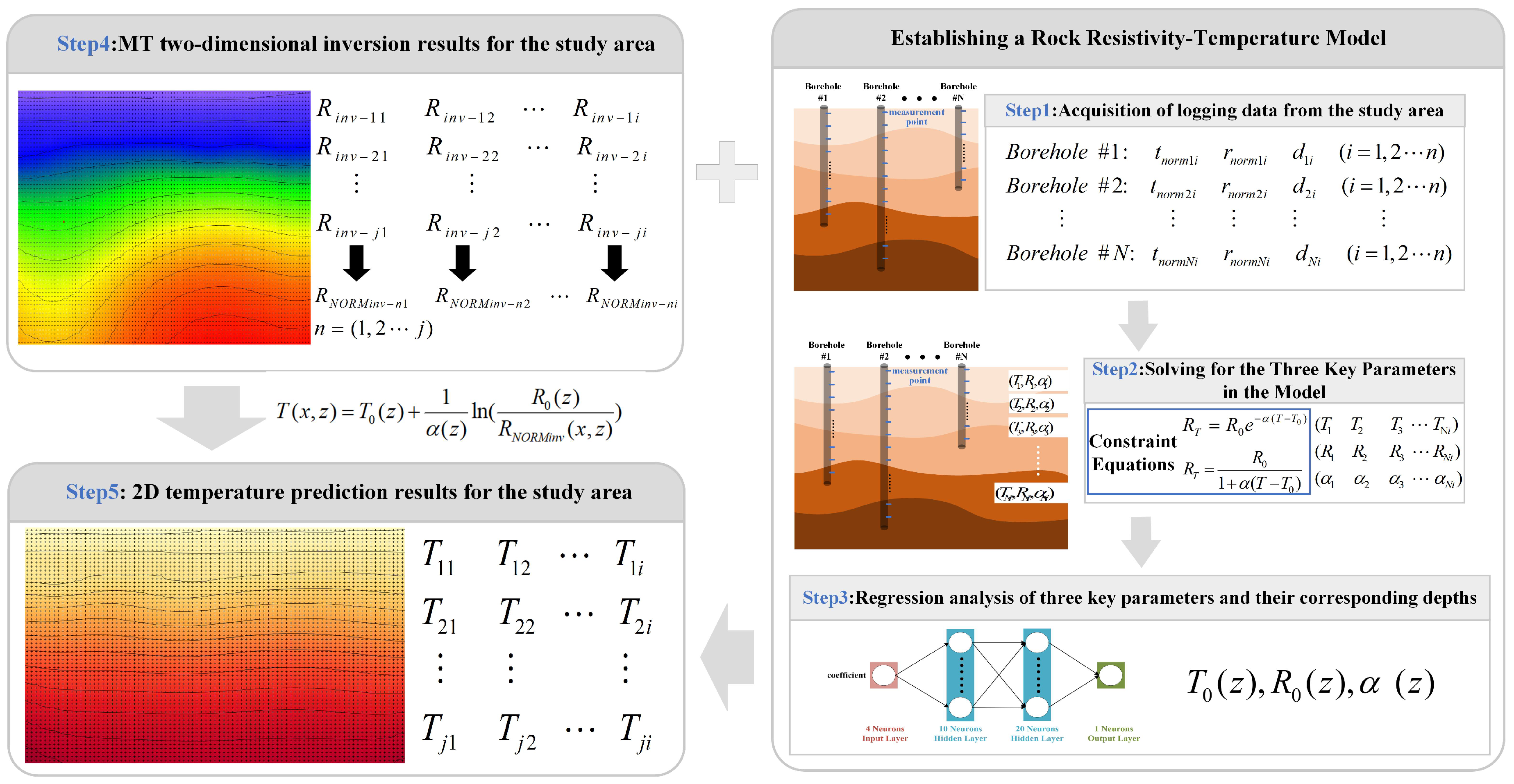
2.2. General Scheme of the RRTCM
3. Prediction of Subsurface Temperatures in the Xiong’an New Area, China
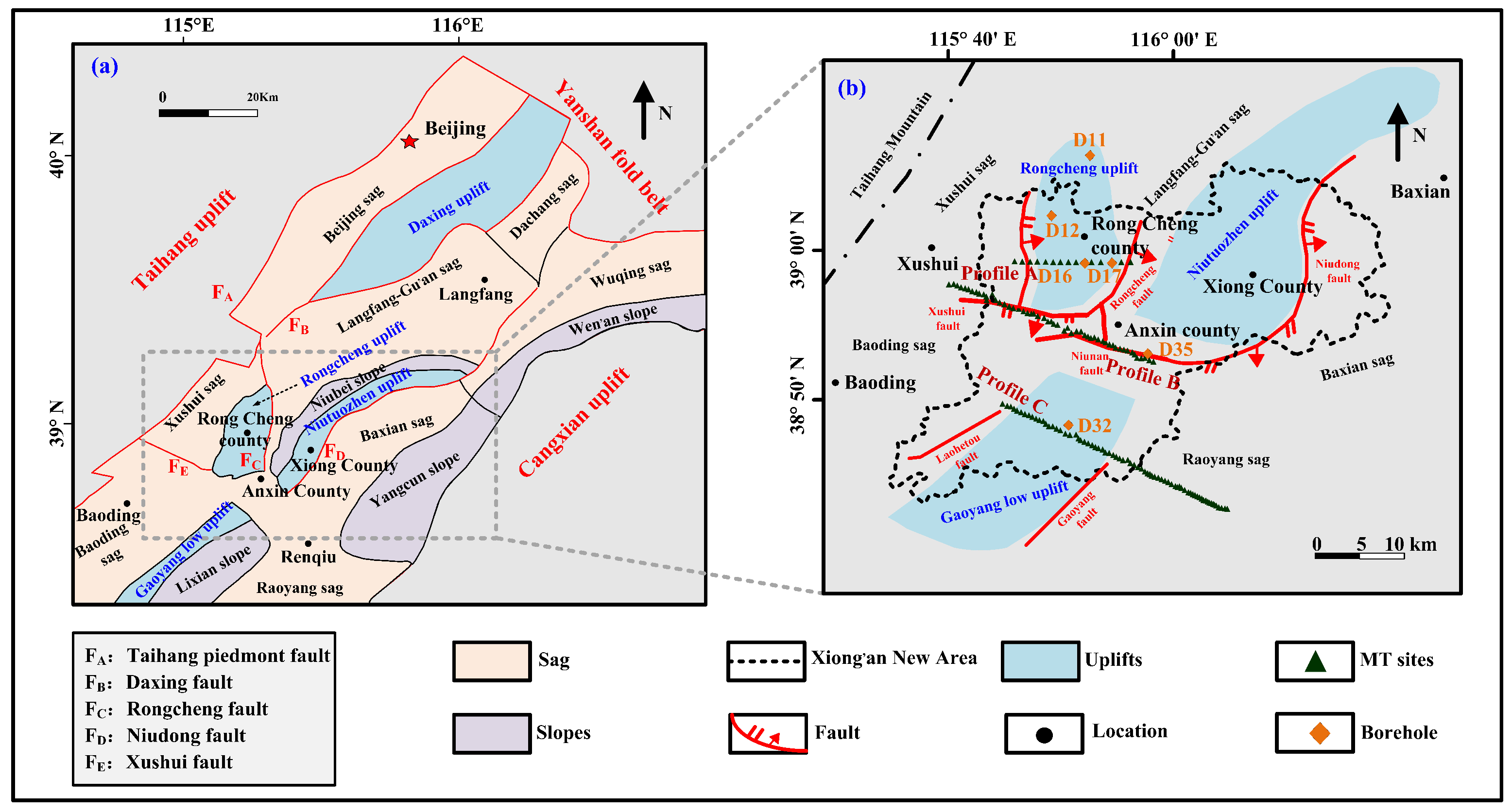
3.1. Geological Setting
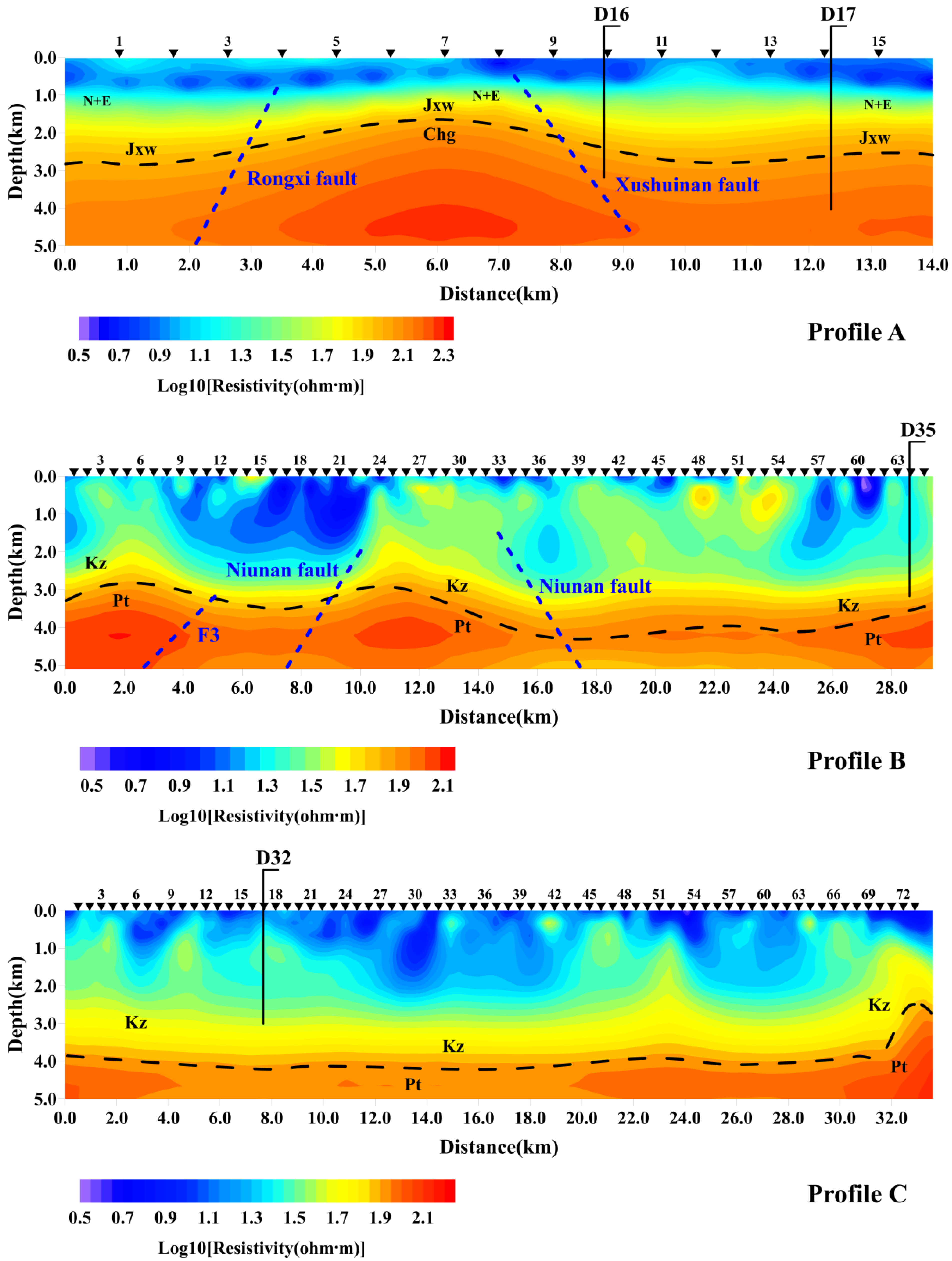
3.2. Results and Analysis
3.3. Method Comparison
- Input layer: 3 neurons (receiving spatial coordinates x, y and resistivity values);
- Hidden layers: Two layers with 20 and 15 neurons, respectively;
- Output layer: 1 neuron (producing predicted temperature values).
4. Analysis of Factors Affecting the Temperature Prediction Accuracy
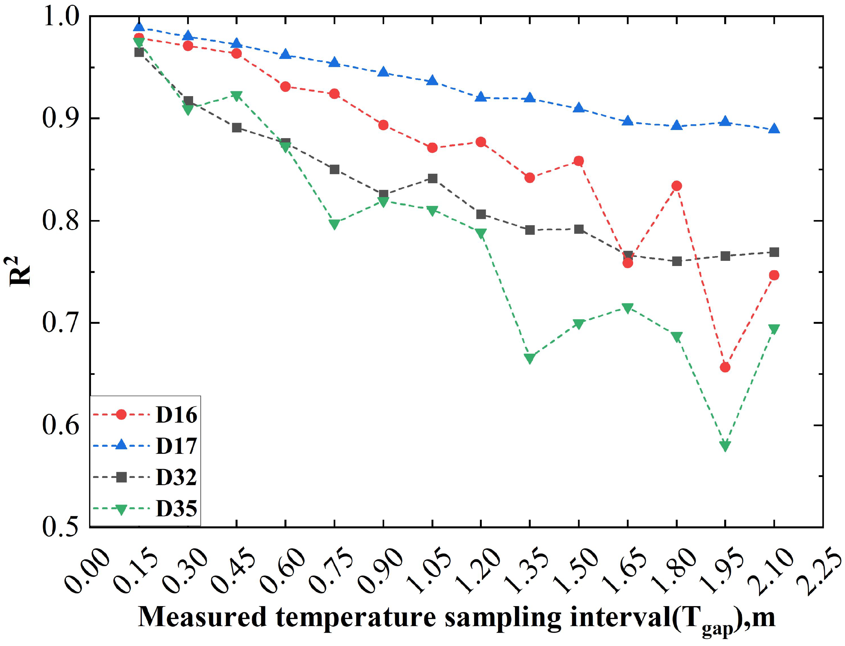
4.1. Effect of the Sampling Interval of the Logging Data from the Constrained Boreholes
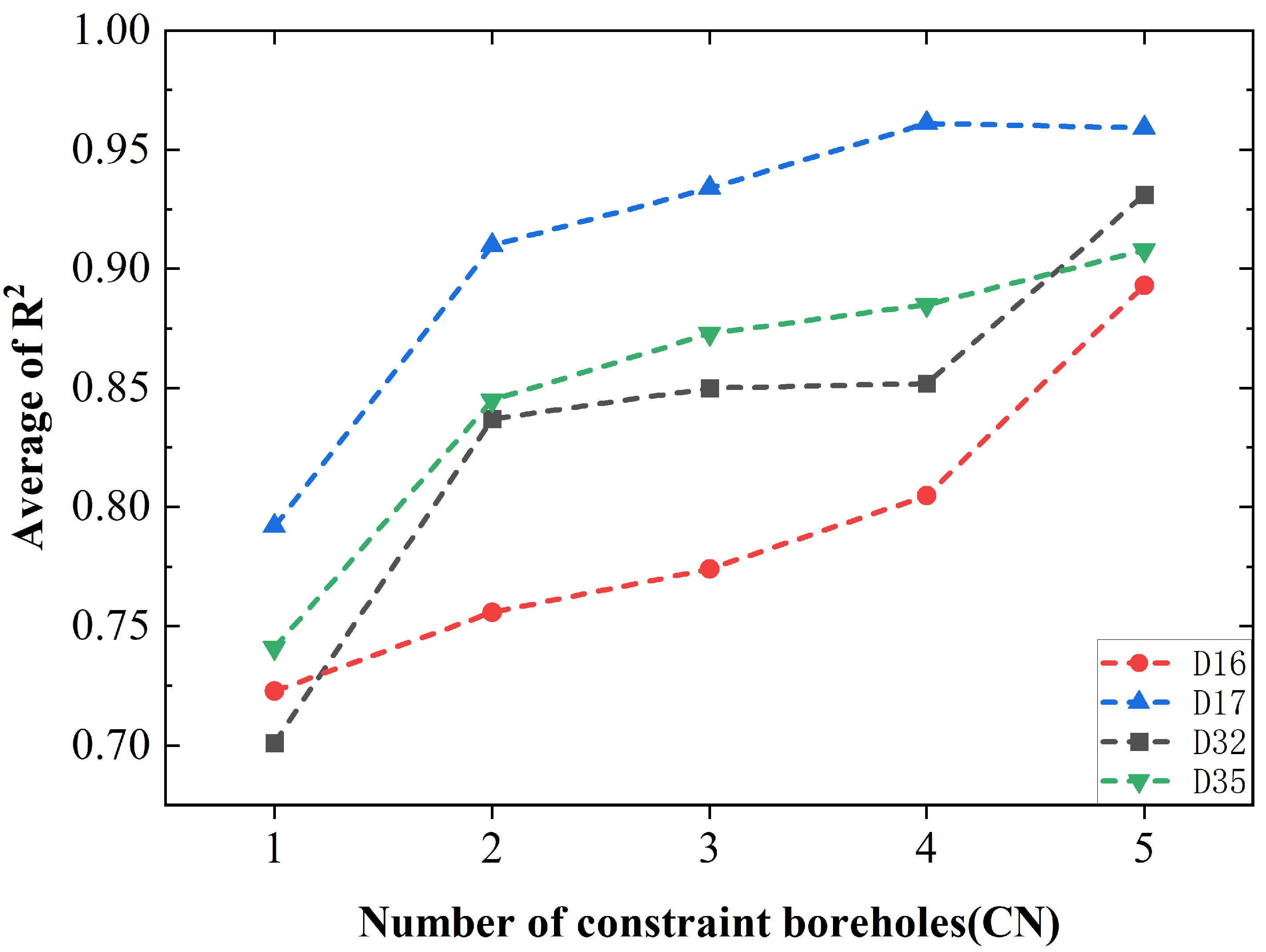
4.2. Effects of the Number of Constrained Boreholes CN and Their Locations
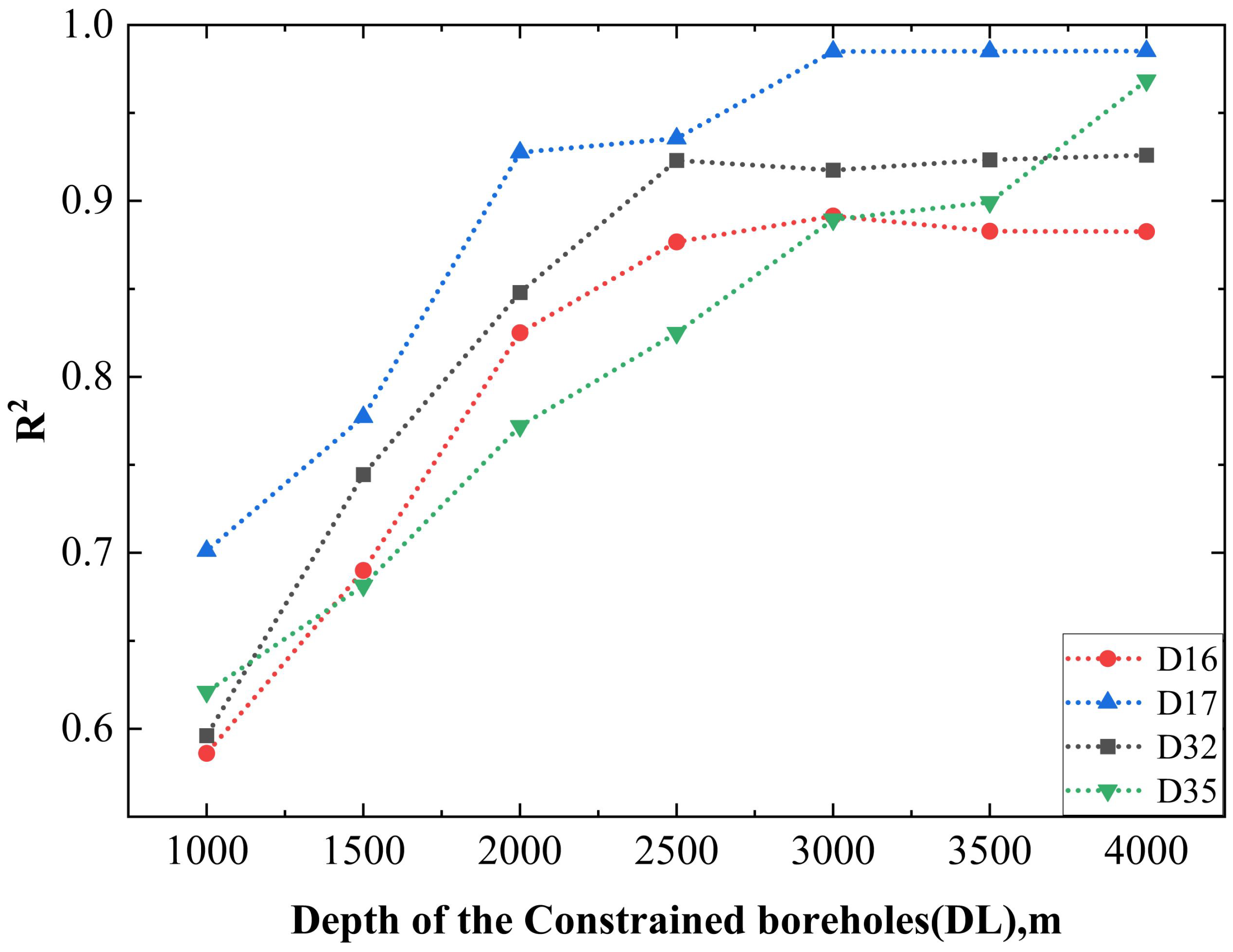
4.3. Effect of the Maximum Depth of the Constrained Boreholes
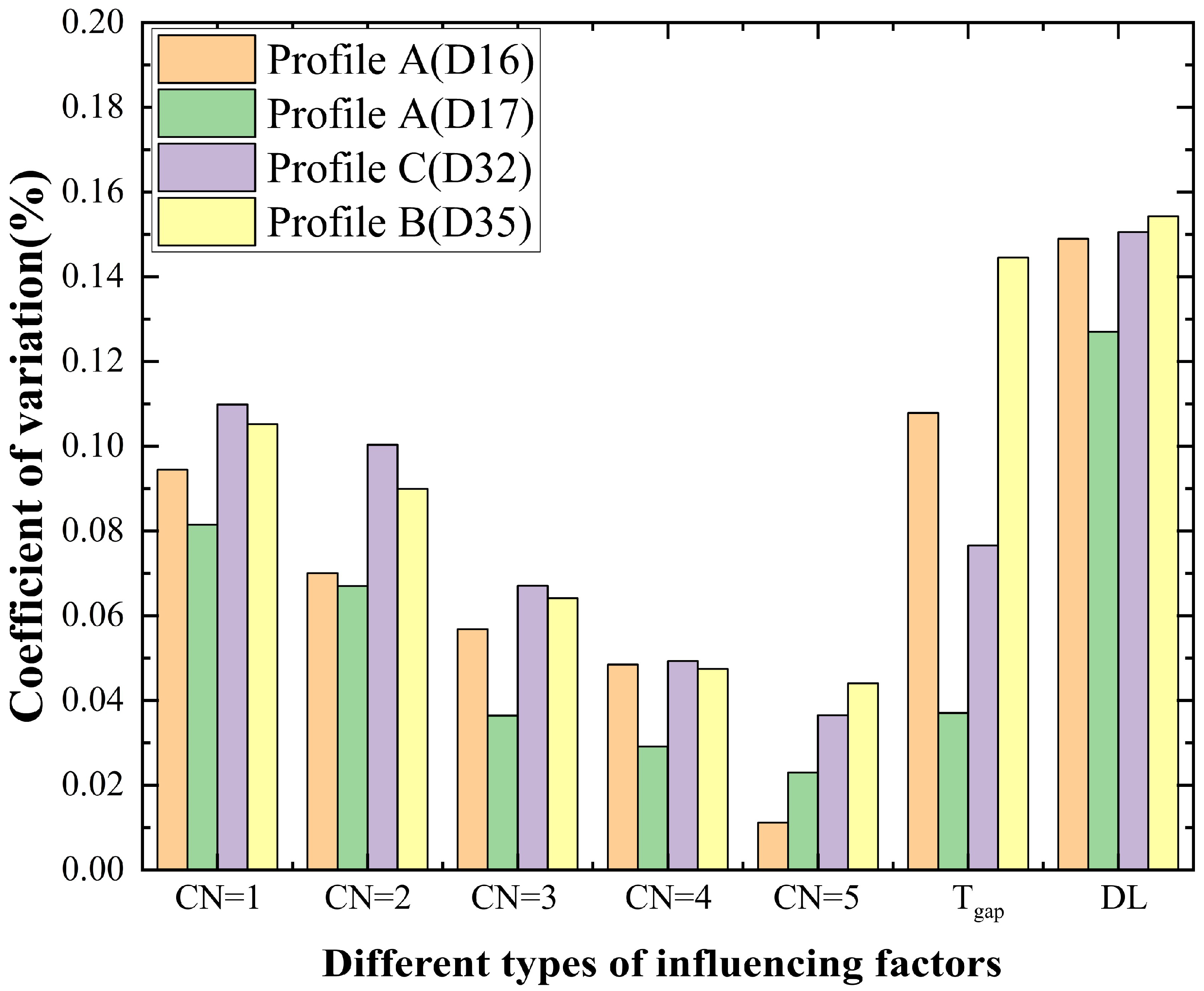
4.4. Comprehensive Comparison of the Sensitivity Analysis Results
5. Conclusions
- Quality of MT data: The accuracy of RRTCM predictions is directly dependent on the resolution and reliability of magnetotelluric inversion results. In areas with strong electromagnetic noise or complex 3D structures, the method’s performance may be compromised.
- Geological complexity: In regions with highly heterogeneous lithology or complex fluid systems, the relationship between resistivity and temperature might deviate significantly from the empirical formulas used in RRTCM, potentially leading to less accurate predictions. In fault zones, particularly those with extensive fracturing or significant displacement, the thermal conductivity and heat flow within the rocks may become heterogeneous, thereby rendering the empirical formula ineffective and preventing the RRTCM from providing accurate temperature predictions.
- Depth limitations: The prediction depth of RRTCM is constrained by the effective penetration depth of MT signals. For very deep temperature predictions (typically >10 km), other methods such as thermal modeling or integrated geophysical approaches might be more suitable.
- Data availability: While RRTCM can achieve good results with relatively few boreholes, it requires both high-quality MT data and temperature-resistivity logging data. In areas where such data are limited or unavailable, machine learning methods that can utilize other types of geophysical data might be more practical.
Author Contributions
Funding
Data Availability Statement
Conflicts of Interest
Abbreviations
| RRTCM | the rock resistivity–temperature coupling model |
| ANNs | artificial neural networks |
| MT | magnetotelluric |
| TCC | temperature compensation coefficient |
| RCC | resistivity compensation coefficient |
| TRCC | temperature–resistivity correction coefficient |
| temperature compensation coefficient | |
| resistivity compensation coefficient | |
| temperature–resistivity correction coefficient | |
| The relationships between the changes in with depth | |
| The relationships between the changes in with depth | |
| The relationships between the changes in with depth | |
| apparent resistivity at the subsurface spatial location P(x, z) | |
| normalized apparent resistivities | |
| the sampling interval of the logging data for the constrained boreholes | |
| the number of constrained boreholes | |
| the maximum depth of the constrained boreholes | |
| coefficient of variation | |
| standard deviation | |
| mean value | |
| total number of samples | |
| TE | transverse electric |
| TM | transverse magnetic |
| Kz | Cenozoic strata |
| Pt | Proterozoic basement rock |
References
- Fridleifsson, I.B.; Freeston, D.H. Geothermal energy research and development. Geothermics 1994, 23, 175–214. [Google Scholar]
- Spichak, V.V.; Zakharova, O.K. Electromagnetic Geothermometry; Elsevier: Amsterdam, The Netherlands, 2015. [Google Scholar]
- Armstead, H.C.H. Geothermal energy development. Prog. Energy Combust. Sci. 1977, 2, 181–238. [Google Scholar]
- Revil, A.; Finizola, A.; Ricci, T.; Delcher, E.; Peltier, A.; Barde-Cabusson, S.; Avard, G.; Bailly, T.; Bennati, L.; Byrdina, S.; et al. Hydrogeology of Stromboli volcano, Aeolian Islands (Italy) from the interpretation of resistivity tomograms, self-potential, soil temperature and soil CO2 concentration measurements. Geophys. J. Int. 2011, 186, 1078–1094. [Google Scholar]
- Zhou, W.; Hu, X.; Yan, S.; Guo, H.; Chen, W.; Liu, S.; Miao, C. Genetic analysis of geothermal resources and geothermal geological characteristics in Datong Basin, Northern China. Energies 2020, 13, 1792. [Google Scholar] [CrossRef]
- Duvillard, P.A.; Magnin, F.; Revil, A.; Legay, A.; Ravanel, L.; Abdulsamad, F.; Coperey, A. Temperature distribution in a permafrost-affected rock ridge from conductivity and induced polarization tomography. Geophys. J. Int. 2021, 225, 1207–1221. [Google Scholar] [CrossRef]
- Pavez, M.; Diaz, D.; Brasse, H.; Kapinos, G.; Budach, I.; Goldberg, V.; Morata, D.; Schill, E. Shallow and deep electric structures in the Tolhuaca geothermal system (S. Chile) investigated by magnetotellurics. Remote Sens. 2022, 14, 6144. [Google Scholar] [CrossRef]
- Ucok, H.; Ershaghi, I.; Olhoeft, G.R. Electrical resistivity of geothermal brines. J. Pet. Technol. 1980, 32, 717–727. [Google Scholar]
- Shankland, T.; Waff, H. Partial melting and electrical conductivity anomalies in the upper mantle. J. Geophys. Res. 1977, 82, 5409–5417. [Google Scholar]
- Tschirhart, V.; Colpron, M.; Craven, J.; Ghalati, F.H.; Enkin, R.J.; Grasby, S.E. Geothermal exploration in the Burwash Landing region, Canada, using three-dimensional inversion of passive electromagnetic data. Remote Sens. 2022, 14, 5963. [Google Scholar] [CrossRef]
- He, L.; Chen, L.; Dorji; Xi, X.; Zhao, X.; Chen, R.; Yao, H. Mapping the geothermal system using AMT and MT in the Mapamyum (QP) field, Lake Manasarovar, Southwestern Tibet. Energies 2016, 9, 855. [Google Scholar] [CrossRef]
- Zhou, W.; Hu, X.; Guo, H.; Liu, S.; Liu, S.; Yang, B. Three-dimensional magnetotelluric inversion reveals the typical geothermal structure of Yanggao geothermal field in Datong Basin, northern China. Geothermics 2022, 105, 102505. [Google Scholar] [CrossRef]
- Corbo-Camargo, F.; Arzate, J.; Fregoso, E.; Norini, G.; Carrasco-Núñez, G.; Yutsis, V.; Herrera, J.; Hernández, J. Shallow structure of Los Humeros (LH) caldera and geothermal reservoir from magnetotellurics and potential field data. Geophys. J. Int. 2020, 223, 666–675. [Google Scholar] [CrossRef]
- Pace, F.; Martí, A.; Queralt, P.; Santilano, A.; Manzella, A.; Ledo, J.; Godio, A. Three-dimensional magnetotelluric characterization of the Travale geothermal field (Italy). Remote Sens. 2022, 14, 542. [Google Scholar] [CrossRef]
- Spichak, V.; Manzella, A. Electromagnetic sounding of geothermal zones. J. Appl. Geophys. 2009, 68, 459–478. [Google Scholar] [CrossRef]
- Singh, R.; Bhoopal, R.; Kumar, S. Prediction of effective thermal conductivity of moist porous materials using artificial neural network approach. Build. Environ. 2011, 46, 2603–2608. [Google Scholar] [CrossRef]
- Spichak, V.; Zakharova, O. The subsurface temperature assessment by means of an indirect electromagnetic geothermometer. Geophysics 2012, 77, WB179–WB190. [Google Scholar] [CrossRef]
- Spichak, V.V.; Zakharova, O.K.; Rybin, A.K. Methodology of the indirect temperature estimation basing on magnetotelluric data: Northern Tien Shan case study. J. Appl. Geophys. 2011, 73, 164–173. [Google Scholar] [CrossRef]
- Maiti, S.; Krishna Tiwari, R.; Kümpel, H.J. Neural network modelling and classification of lithofacies using well log data: A case study from KTB borehole site. Geophys. J. Int. 2007, 169, 733–746. [Google Scholar] [CrossRef]
- Huang, G.; Hu, X.; Cai, J.; Ma, H.; Chen, B.; Liao, C.; Zhang, S.; Zhou, W. Subsurface temperature prediction by means of the coefficient correction method of the optimal temperature: A case study in the Xiong’an New Area, China. Geophysics 2022, 87, B269–B285. [Google Scholar] [CrossRef]
- Huang, G.; Hu, X.; Liu, S.; Peng, R.; Zhou, J.; Bai, N.; Liu, L.; Mu, M. Deep temperature-field prediction utilizing the temperature–pressure coupled resistivity model: A case study in the Xiong’an New Area, China. IEEE Trans. Geosci. Remote Sens. 2023, 62, 5902216. [Google Scholar] [CrossRef]
- Chave, A.D.; Jones, A.G. The Magnetotelluric Method: Theory and Practice; Cambridge University Press: Cambridge, UK, 2012. [Google Scholar]
- Campbell, R.; Bower, C.; Richards, L. Change of electrical conductivity with temperature and the relation of osmotic pressure to electrical conductivity and ion concentration for soil extracts. Soil Sci. Soc. Am. J. 1949, 13, 66–69. [Google Scholar] [CrossRef]
- Keller, G.V.; Frischknecht, F.C. Electrical Methods in Geophysical Prospecting; Pergamon Press: Oxford, UK, 1966. [Google Scholar]
- Eppelbaum, L.; Kutasov, I.; Pilchin, A. Applied Geothermics; Springer: Berlin/Heidelberg, Germany, 2014. [Google Scholar]
- Eppelbaum, L.; Kutasov, I.; Pilchin, A.; Eppelbaum, L.; Kutasov, I.; Pilchin, A. Thermal properties of rocks and density of fluids. In Applied Geothermics; Springer: Berlin/Heidelberg, Germany, 2014; pp. 99–149. [Google Scholar]
- Aiqun, S.; Shuyin, N. The mantle plume evolution and its geothermal effect-deep tectonic setting of geothermal anomaly in North China. Acta Geosci. Sin. 2000, 21, 182–189. [Google Scholar]
- Gao, Y.; Wu, J.; Fukao, Y.; Shi, Y.; Zhu, A. Shear wave splitting in the crust in North China: Stress, faults and tectonic implications. Geophys. J. Int. 2011, 187, 642–654. [Google Scholar]
- Gao, P.; Qiu, Q.; Jiang, G.; Zhang, C.; Hu, S.; Lei, Y.; Wang, X. Present-day geothermal characteristics of the Ordos Basin, western North China Craton: New findings from deep borehole steady-state temperature measurements. Geophys. J. Int. 2018, 214, 254–264. [Google Scholar] [CrossRef]
- Chen, M.; Wang, J.; Wang, J.; Deng, X.; Yang, S.Z.; Xiong, L.; Zhang, J.M. The characteristics of the geothermal field and its formation mechanism in the North China down-faulted basin. Acta Geol. Sin. 1990, 64, 80–91. [Google Scholar]
- Wang, Z.; Jiang, G.; Zhang, C.; Hu, J.; Shi, Y.; Wang, Y.; Hu, S. Thermal regime of the lithosphere and geothermal potential in Xiong’an New Area. Energy Explor. Exploit. 2019, 37, 787–810. [Google Scholar] [CrossRef]
- Cao, Y.; Bao, Z.; Lu, K.; Xu, S.; Wang, G.; Yuan, S.; Ji, H. Genetic model and main controlling factors of the Xiongxian geothermal field. Acta Sedimentol. Sin. 2021, 39, 863–872. [Google Scholar]
- He, D.; Shan, S.; Zhang, Y.; Lu, R.; Zhang, R.; Cui, Y. 3-D geologic architecture of Xiong’an New Area: Constraints from seismic reflection data. Sci. China Earth Sci. 2018, 61, 1007–1022. [Google Scholar]
- Yang, J.; Huang, G.; Hu, X. A 3D thermal conductivity prediction method for deep strata based on temperature field estimation. Geophysics 2023, 88, B297–B316. [Google Scholar]
- Zhang, Q.; Zhu, X.; Wang, G.; Ma, F. Characteristics, Formation Periods, and Controlling Factors of Tectonic Fractures in Carbonate Geothermal Reservoirs: A Case Study of the Jixianian System in the Xiong’an New Area, China. Acta Geol. Sin.-Engl. Ed. 2023, 97, 1625–1639. [Google Scholar]
- Yue, G.; Wang, G.; Ma, F.; Zhang, W.; Yang, Z. The thermal state and geothermal energy accumulation mechanism in the Xiong’an New Area, China. Energy Explor. Exploit. 2019, 37, 1039–1052. [Google Scholar]
- Shi, Z.; Wang, G. Evaluation of the permeability properties of the Xiaojiang Fault Zone using hot springs and water wells. Geophys. J. Int. 2017, 209, 1526–1533. [Google Scholar] [CrossRef]
- Lister, C. On the penetration of water into hot rock. Geophys. J. Int. 1974, 39, 465–509. [Google Scholar] [CrossRef]
- Shang, S. Study on Quaternary Activity of Main Buried Faults and Strata Mineral Composition in Xiong’an New Area and Neighboring Areas. Master’s Thesis, China University of Geosciences (Beijing), Beijing, China, 2020. [Google Scholar]
- Wu, A.; Ma, F.; Wang, G.; Liu, J.; Hu, Q.; Miao, Q. A study of deep-seated karst geothermal reservoir exploration and huge capacity geothermal well parameters in Xiongan New Area. Acta Geosci. Sin. 2018, 39, 523–532. [Google Scholar]
- Guo, S.; Zhu, C.; Qiu, N.; Tang, B.; Cui, Y.; Zhang, J.; Zhao, Y. Present geothermal characteristics and influencing factors in the Xiong’an New Area, North China. Energies 2019, 12, 3884. [Google Scholar] [CrossRef]
- Rodi, W.; Mackie, R.L. Nonlinear conjugate gradients algorithm for 2-D magnetotelluric inversion. Geophysics 2001, 66, 174–187. [Google Scholar] [CrossRef]
- Hansen, P.C. Analysis of discrete ill-posed problems by means of the L-curve. SIAM Rev. 1992, 34, 561–580. [Google Scholar] [CrossRef]
- Berdichevsky, M.N.; Dmitriev, V.I. Magnetotelluric sounding of geological structures. Methods Geochem. Geophys. 1998, 37, 1–377. [Google Scholar]
- Wannamaker, P.E.; Hohmann, G.W.; Ward, S.H. Magnetotelluric responses of three-dimensional bodies in layered earths. Geophysics 1984, 49, 1517–1533. [Google Scholar] [CrossRef]
- Parkhomenko, E. Electrical resistivity of minerals and rocks at high temperature and pressure. Rev. Geophys. 1982, 20, 193–218. [Google Scholar] [CrossRef]


| CN | Constrained Borehole Combination | Constraint Data (Borehole) | Max (GOF) | Min (GOF) | Avg (GOF) | |||||
|---|---|---|---|---|---|---|---|---|---|---|
| D11 | D12 | D16 | D17 | D32 | D35 | |||||
| 1 | C101 | √ | 0.832 | 0.626 | 0.726 | |||||
| C102 | √ | 0.629 | 0.561 | 0.603 | ||||||
| C103 | √ | 0.912 | 0.752 | 0.816 | ||||||
| C104 | √ | 0.925 | 0.759 | 0.814 | ||||||
| C105 | √ | 0.804 | 0.719 | 0.770 | ||||||
| C106 | √ | 0.886 | 0.627 | 0.708 | ||||||
| 2 | C201 | √ | √ | 0.962 | 0.697 | 0.809 | ||||
| C202 | √ | √ | 0.931 | 0.717 | 0.806 | |||||
| C203 | √ | √ | 0.937 | 0.750 | 0.810 | |||||
| C204 | √ | √ | 0.924 | 0.768 | 0.858 | |||||
| C205 | √ | √ | 0.942 | 0.651 | 0.758 | |||||
| C206 | √ | √ | 0.936 | 0.754 | 0.855 | |||||
| C207 | √ | √ | 0.921 | 0.760 | 0.819 | |||||
| C208 | √ | √ | 0.934 | 0.726 | 0.814 | |||||
| C209 | √ | √ | 0.928 | 0.809 | 0.887 | |||||
| C210 | √ | √ | 0.908 | 0.758 | 0.813 | |||||
| C211 | √ | √ | 0.941 | 0.711 | 0.874 | |||||
| C212 | √ | √ | 0.955 | 0.647 | 0.841 | |||||
| C213 | √ | √ | 0.952 | 0.812 | 0.874 | |||||
| C214 | √ | √ | 0.996 | 0.804 | 0.870 | |||||
| C215 | √ | √ | 0.948 | 0.765 | 0.866 | |||||
| 3 | C301 | √ | √ | √ | 0.942 | 0.767 | 0.833 | |||
| C302 | √ | √ | √ | 0.935 | 0.753 | 0.817 | ||||
| C303 | √ | √ | √ | 0.950 | 0.782 | 0.867 | ||||
| C304 | √ | √ | √ | 0.954 | 0.792 | 0.880 | ||||
| C305 | √ | √ | √ | 0.917 | 0.760 | 0.809 | ||||
| C306 | √ | √ | √ | 0.958 | 0.733 | 0.876 | ||||
| C307 | √ | √ | √ | 0.963 | 0.666 | 0.833 | ||||
| C308 | √ | √ | √ | 0.957 | 0.814 | 0.869 | ||||
| C309 | √ | √ | √ | 0.951 | 0.783 | 0.849 | ||||
| C310 | √ | √ | √ | 0.930 | 0.781 | 0.870 | ||||
| C311 | √ | √ | √ | 0.911 | 0.772 | 0.820 | ||||
| C312 | √ | √ | √ | 0.941 | 0.741 | 0.882 | ||||
| C313 | √ | √ | √ | 0.965 | 0.728 | 0.871 | ||||
| C314 | √ | √ | √ | 0.967 | 0.817 | 0.881 | ||||
| C315 | √ | √ | √ | 0.960 | 0.825 | 0.870 | ||||
| C316 | √ | √ | √ | 0.957 | 0.771 | 0.865 | ||||
| C317 | √ | √ | √ | 0.964 | 0.781 | 0.867 | ||||
| C318 | √ | √ | √ | 0.948 | 0.763 | 0.846 | ||||
| C319 | √ | √ | √ | 0.944 | 0.713 | 0.873 | ||||
| C320 | √ | √ | √ | 0.942 | 0.812 | 0.881 | ||||
| 4 | C401 | √ | √ | √ | √ | 0.919 | 0.774 | 0.817 | ||
| C402 | √ | √ | √ | √ | 0.959 | 0.762 | 0.886 | |||
| C403 | √ | √ | √ | √ | 0.975 | 0.738 | 0.863 | |||
| C404 | √ | √ | √ | √ | 0.940 | 0.822 | 0.869 | |||
| C405 | √ | √ | √ | √ | 0.988 | 0.805 | 0.869 | |||
| C406 | √ | √ | √ | √ | 0.924 | 0.800 | 0.880 | |||
| C407 | √ | √ | √ | √ | 0.980 | 0.784 | 0.865 | |||
| C408 | √ | √ | √ | √ | 0.974 | 0.764 | 0.846 | |||
| C409 | √ | √ | √ | √ | 0.953 | 0.805 | 0.895 | |||
| C410 | √ | √ | √ | √ | 0.984 | 0.813 | 0.886 | |||
| C411 | √ | √ | √ | √ | 0.976 | 0.827 | 0.883 | |||
| C412 | √ | √ | √ | √ | 0.973 | 0.825 | 0.873 | |||
| C413 | √ | √ | √ | √ | 0.945 | 0.803 | 0.897 | |||
| C414 | √ | √ | √ | √ | 0.982 | 0.820 | 0.895 | |||
| C415 | √ | √ | √ | √ | 0.985 | 0.855 | 0.912 | |||
| 5 | C501 | √ | √ | √ | √ | √ | 0.980 | 0.861 | 0.922 | |
| C502 | √ | √ | √ | √ | √ | 0.922 | 0.882 | 0.897 | ||
| C503 | √ | √ | √ | √ | √ | 0.954 | 0.890 | 0.918 | ||
| C504 | √ | √ | √ | √ | √ | 0.973 | 0.881 | 0.925 | ||
| C505 | √ | √ | √ | √ | √ | 0.975 | 0.894 | 0.925 | ||
| C506 | √ | √ | √ | √ | √ | 0.975 | 0.909 | 0.950 | ||
| Constrained Boreholes | Profile A (km) | Profile B (km) | Profile C (km) |
|---|---|---|---|
| D11 | 12.6 | 20.2 | 31.4 |
| D12 | 4.5 | 11.5 | 22.7 |
| D16 | 0.3 | 7.7 | 19.1 |
| D17 | 0.2 | 9.1 | 20.7 |
| D32 | 21.9 | 12.4 | 0.6 |
| D35 | 11.4 | 0.9 | 12.9 |
Disclaimer/Publisher’s Note: The statements, opinions and data contained in all publications are solely those of the individual author(s) and contributor(s) and not of MDPI and/or the editor(s). MDPI and/or the editor(s) disclaim responsibility for any injury to people or property resulting from any ideas, methods, instructions or products referred to in the content. |
© 2025 by the authors. Licensee MDPI, Basel, Switzerland. This article is an open access article distributed under the terms and conditions of the Creative Commons Attribution (CC BY) license (https://creativecommons.org/licenses/by/4.0/).
Share and Cite
Wang, R.; Huang, G.; Yang, J.; Liu, L.; Luo, W.; Hu, X. A Precise Prediction Method for Subsurface Temperatures Based on the Rock Resistivity–Temperature Coupling Model. Remote Sens. 2025, 17, 1331. https://doi.org/10.3390/rs17081331
Wang R, Huang G, Yang J, Liu L, Luo W, Hu X. A Precise Prediction Method for Subsurface Temperatures Based on the Rock Resistivity–Temperature Coupling Model. Remote Sensing. 2025; 17(8):1331. https://doi.org/10.3390/rs17081331
Chicago/Turabian StyleWang, Ri, Guoshu Huang, Jian Yang, Lichao Liu, Wang Luo, and Xiangyun Hu. 2025. "A Precise Prediction Method for Subsurface Temperatures Based on the Rock Resistivity–Temperature Coupling Model" Remote Sensing 17, no. 8: 1331. https://doi.org/10.3390/rs17081331
APA StyleWang, R., Huang, G., Yang, J., Liu, L., Luo, W., & Hu, X. (2025). A Precise Prediction Method for Subsurface Temperatures Based on the Rock Resistivity–Temperature Coupling Model. Remote Sensing, 17(8), 1331. https://doi.org/10.3390/rs17081331