Neural Network-Based Temporal Ensembling of Water Depth Estimates Derived from SuperDove Images

Abstract

CubeSats provide a wealth of high-frequency observations at a meter-scale spatial resolution. However, most current methods of inferring water depth from satellite data consider only a single image. This approach is sensitive to the radiometric quality of the data acquired at that particular instant in time, which could be degraded by various confounding factors, such as sun glint or atmospheric effects. Moreover, using single images in isolation fails to exploit recent improvements in the frequency of satellite image acquisition. This study aims to leverage the dense image time series from the SuperDove constellation via an ensembling framework that helps to improve empirical (regression-based) bathymetry retrieval. Unlike previous studies that only ensembled the original spectral data, we introduce a neural network-based method that instead ensembles the water depths derived from multi-temporal imagery, provided the data are acquired under steady flow conditions. We refer to this new approach as NN-depth ensembling. First, every image is treated individually to derive multitemporal depth estimates. Then, we use another NN regressor to ensemble the temporal water depths. This step serves to automatically weight the contribution of the bathymetric estimates from each time instance to the final bathymetry product. Unlike methods that ensemble spectral data, NN-depth ensembling mitigates against propagation of uncertainties in spectral data (e.g., noise due to sun glint) to the final bathymetric product. The proposed NN-depth ensembling is applied to temporal SuperDove imagery of reaches from the American, Potomac, and Colorado rivers with depths of up to 10 m and evaluated against in situ measurements. The proposed method provided more accurate and robust bathymetry retrieval than single-image analyses and other ensembling approaches.

1. Introduction

Earth observation has entered a new era with the advent of CubeSat constellations, which provide imagery with global coverage at meter-scale resolution and with the objective of daily or even sub-daily revisit times [1]. The availability of images with such high spatial and temporal resolution results from the development of fleets that consist of a large number (hundreds) of small satellites. PlanetScope Doves provided first-of-its-kind CubeSat constellations imaging the Earth’s landmass on a daily basis with ~3 m spatial resolution and four spectral channels [2]. The follow-up mission has taken an additional step further by launching a new generation of CubeSats called SuperDoves that enhance the spectral resolution by capturing eight spectral bands within the visible and near-infrared portion of the spectrum. The spectral bands of SuperDoves are narrower than those of earlier-generation Doves, and the additional bands include coastal blue (443 nm), extra green (531 nm), yellow (610 nm), and red edge (705 nm) channels [3]. A key characteristic of both the Dove and SuperDove constellations is their ability to provide abundant cloud-free images. This capability has been made possible by a large number of CubeSats (>150 SuperDoves currently in orbit) deployed in two specially designed near-polar orbits. The orbits have opposite inclinations that scan the Earth through both ascending and descending orbits. There is a swath overlap between subsequent CubeSats in each orbit, allowing for the capture of images only 90 s apart. Moreover, the Planet constellation provides other sub-daily imagery with time lags ranging from a few minutes to a few hours, given that the image acquisitions are from both ascending and descending orbits [1,4]. Thus, the Planet CubeSat constellation allows for the unprecedented capture of daily and sub-daily images with global coverage at high spatial resolution. The frequent revisits increase the likelihood of capturing cloud-free conditions. The wealth of temporal imagery from CubeSats can potentially bring new opportunities in remote sensing of aquatic systems from both methodological and application-oriented perspectives.

The radiometric quality of optical imagery is of particular importance in aquatic applications [5]. This is because water bodies typically have very low reflectance, and thus the water-leaving radiance is a small portion (<15%) of the at-sensor radiance and can be severely contaminated by confounding factors such as atmospheric effects and sun glint from the water surface [6,7]. Thus, sensors with high radiometric sensitivity are needed to resolve subtle variations in water-leaving radiance, which are linked to the variation in biophysical parameters of interest (e.g., bathymetry and concentration of constituents) [8]. Doves and SuperDoves record spectral information with a relatively high radiometric resolution (12-bit). However, CubeSats carry small and inexpensive sensors; thus, the radiometric quality might not be as consistent as standard, larger sensors like those onboard Landsat-8/9 and Sentinel-2A/B [9,10]. Despite these concerns about the radiometric quality, CubeSat data have already proven promising in retrieving water depth and turbidity [11,12].

Bathymetry retrieval in inland waters, including fluvial systems, is essential for flood risk assessment, environmental conservation, and infrastructure planning. Information on water depth also supports habitat modeling and preservation of aquatic ecosystems [13,14]. CubeSat imagery has become increasingly appealing to aquatic scientists and managers, particularly those working in inland waters due to the high spatial and temporal resolution of these data [15]. The meter-scale resolution allows even small water bodies to be captured, such as river channels, that cannot be resolved at the spatial resolution of publicly available satellite images (e.g., 10–30 m for Sentinel-2A/B and Landsat-8/9). Although commercial spaceborne missions like WorldView provide meter-scale spatial resolution, these data are only acquired on a tasked, on-demand basis, as opposed to routine daily imaging by CubeSats at the global scale. The daily (sub-daily) imagery offered by CubeSats enhances the chance to capture cloud-free imagery and monitor changes in a timely manner. Because the SuperDove imagery has been available only since early 2022, previous studies conducted in aquatic systems are mostly based on four-band Dove data (e.g., [9,11,15]). For instance, Dove data provided promising results in mapping water turbidity in San Franciso Bay, USA, and coastal waters around the UK [11]. Bathymetry retrieval using Dove imagery has been performed with promising results in coastal waters [16] and rivers [12].

The spectrally based methods for standard bathymetry retrieval from single images fall into two main approaches: physics-based and empirical [17,18,19,20]. Physics-based models require an atmospheric correction designed for aquatic applications to derive accurate remote sensing reflectance (R_rs) data [21]. Moreover, information on water column optical properties and bottom reflectance are needed to perform the inversion of a radiative transfer model [21,22,23,24,25]. On the other hand, empirical methods allow for estimating bathymetry by developing a regression model that relates spectral characteristics to depths measured in the field. Empirical models are more straightforward to apply because there is no need to model the underlying physics. Thus, they can be applied to top-of-atmosphere (TOA) data without characterizing the water column’s bio-optical conditions and substrate properties. This study builds upon the regression-based approach for bathymetry retrieval. The literature covers a range of regression models employed for water depth retrieval, from different forms of band ratio models [26] to more recent machine learning techniques like the neural network-based depth retrieval (NNDR) technique. Here, we leverage NNDR as a state-of-the-art technique that provided promising results in previous studies [12,27]. We incorporate NNDR into a new methodology for temporal ensembling of SuperDove imagery.

This study focuses on empirical bathymetry retrieval from newly available SuperDoves and introduces a machine learning-based model for ensembling depth estimates from dense time series of images. In a recent study, we exploited four-band Dove image sequences with short time lags (from seconds to hours) by averaging spectral data (mean–spec ensembling) to improve bathymetry retrieval relative to the standard single-image analysis [12]. Time-averaging the original spectral data has been the predominant ensembling technique in prior studies, with the goal of leveraging temporal imagery to enhance bathymetry retrieval [12,28]. Here, we introduce an alternative approach that performs the ensembling on the bathymetry products derived from individual images rather than ensembling the spectral data first and then proceeding to depth retrieval. Although empirical methods do not require absolute radiance values, the spectral data must at least be internally consistent in order to obtain an accurate and robust regression model. However, confounding factors like the surface glint and water column optical properties vary not only in space but also in time. Consequently, the adverse effects of these factors are amplified when the spectral data are directly ensembled over time. The pixel-by-pixel consistency of a time-averaged image created by mean–spec ensembling can thus be degraded by any variations in confounding factors present in the multitemporal data. For example, variability in atmospheric effects can lead to pronounced artifacts in the time-averaged image, particularly when the time series spans a longer period of several days. Moreover, this issue can be exacerbated by any radiometric inconsistencies among different SuperDove sensors. The rationale behind the proposed ensembling is to mitigate the propagation of any or all of these confounding factors by treating the images individually at the first step and then ensembling the resulting depth estimates over time. The foundation of this approach is a neural network (NN) regressor (NN–depth ensembling) that essentially weights the contribution of the depth estimates from each time period to derive the final depth estimate at each location. This study addresses the following objectives: (i) develop a neural network (NN)-based method for ensembling temporal retrievals of water depth (NN–depth ensembling) from dense time-series of SuperDove imagery; (ii) compare the performance of the proposed NN–depth ensembling relative to the mean–spec and average depth (mean–depth) ensembling approaches, as well as standard single-image analysis; and (iii) perform bathymetry retrieval in a wide range of water depths in multiple case studies to evaluate the performance of the proposed NN–depth ensembling. This study also provides more insights into the utility of the newly available SuperDove imagery for bathymetric applications. Section 2 describes the proposed NN–depth ensembling method along with other ensembling techniques. The case studies and the datasets are introduced in Section 3. The results and discussions are provided in Section 4. The manuscript concludes in Section 5 by providing a summary and suggesting directions for additional studies.

2. Methods

Let $\{I_1,I_2,\dots ,I_T\}$ represent a set of temporally dense images of the same area captured by CubeSats at time instances t₁ to t_T. We assume that flow conditions remain relatively steady throughout the time period over which these images are acquired and that in situ bathymetry data (d) from one of these time instances are available for use in developing the NN model. Note that in coastal waters, applying a tide correction to a datum like mean sea level helps maintain consistent bathymetry across the time period when images are acquired. We split the field measurements into training (d_Train) and validation (d_Val) sets. In a recent study, the authors proposed spectral averaging of short time lag (from seconds to hours) image sequences from Dove CubeSats as a means of ensembling and showed that this approach improves bathymetry retrieval relative to standard single-image analysis [12]. We refer to this method as mean–spec ensembling hereafter. Thus, the spectrally averaged image at a given wavelength (λ) can be derived as:

$$\overline{I\left(\lambda \right)}={\displaystyle \frac{{\sum }_{t=1}^T{I}_t\left(\lambda \right)}{T}}$$

(1)

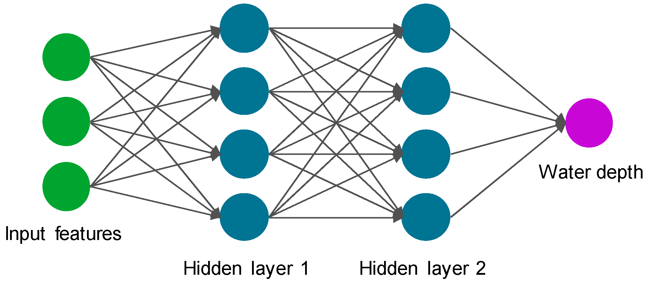
The mean–spec ensembling approach retrieves the bathymetry by training a NN depth retrieval (NNDR) model on the time-averaged image [12,27]. NN-based regressors automate the process of feature extraction and account for complex nonlinear relations among the features and response variables [29]. The NNDR is trained by considering the spectral bands for the training samples $\overline{I(\lambda ,x)}$ as input features and associated in situ depths d_Train (x) as the network’s response variable, where x denotes the spatial location of a training sample. NNDR is a fully connected network with two hidden layers. Bayesian optimization is employed to tune the hyperparameters of NNDR, including the number of neurons in each layer and the type of activation function [30,31]. The hyperparameter tuning runs through layer sizes of up to 100 neurons to find the optimal size by minimizing the cross-validation error. The rectified linear unit (ReLU) is identified as an optimal activation function that effectively handles gradient explosion and disappearance [32]. Figure 1 schematically illustrates the NNDR architecture.

This approach performs the time averaging on the spectral data (mean–spec) before performing any depth retrieval. The originally developed mean–spec ensembling leveraged CubeSat imagery only with short time lags to ensure relatively steady conditions in terms of water depth, water surface glint, and atmospheric effects [12]. The temporal consistency of spectral data can be degraded due to variations in sun glint from the water surface, atmospheric effects, optical properties of the water column, and possibly inter-sensor radiometric inconsistencies between individual SuperDoves. As a result, approaches such as mean–spec that ensemble the spectral data are subject to temporally aggregated confounding factors. To tackle this issue, we propose an alternative approach that involves ensembling at the product level on the time series of bathymetry estimates. The proposed NN-depth ensembling first retrieves bathymetry independently for each image in the time series, employing a separate NNDR for each time instance (NNDR₁ to NNDR_T) that uses {I_t (x), d_Train (x)} for training. Then, the temporal estimates of depths for training samples D_t(x) are fed as features into another NNDR_Ens with field measurements as the response d_Train(x). The structure of NNDR_Ens is similar to the NNDR, but the input features are different. NNDR_Ens performs the ensembling by regressing the initial round of temporal depth estimates {D₁(x), D₂(x), …, D_T(x)} against the corresponding in situ values d_Train(x). Thus, the number of input features for the NNDR_Ens is equal to the number of time instances T. Because the ensembling is based on a NN regressor rather than simple averaging, the proposed ensembling allows for automatic weighting of the contribution of depths estimated at different time instances into the final bathymetry product. Moreover, the depth-to-depth (input-to-output) ensembling provides a means of compensating for errors in the D_t, particularly any systematic biases. We also implemented a simple averaging of D_t as an alternative ensembling approach (mean–depth) for comparison purposes. In this case, the time-averaged depths ($\overline{D}$) can be derived as follows:

$$\overline{D}={\displaystyle \frac{{\sum }_{t=1}^T{D}_t}{T}}$$

(2)

Figure 2 provides a schematic representation of three ensembling approaches to leverage temporally dense imagery from CubeSats in bathymetry retrieval. For consistency among different analyses, whether based on single images or on one of the ensembling approaches, the training samples d_Train(x) remain the same for all the NNs involved at each stage of the various ensemble-based methods. We also use the same validation set (d_Val) to evaluate all cases. The training is repeated ten times for all NNs, and the estimates resulting from these ten replicates are averaged to produce the final retrievals. The implementation of the NNs is carried out using the Deep Learning Toolbox of the MATLAB (R2024a) software package [33]. Also note that we evaluated using the median rather than the mean for both the mean–spec and the mean–depth approaches, but we found that using the mean outperformed the alternative, median-based workflow. For brevity, results derived using the median are not included.

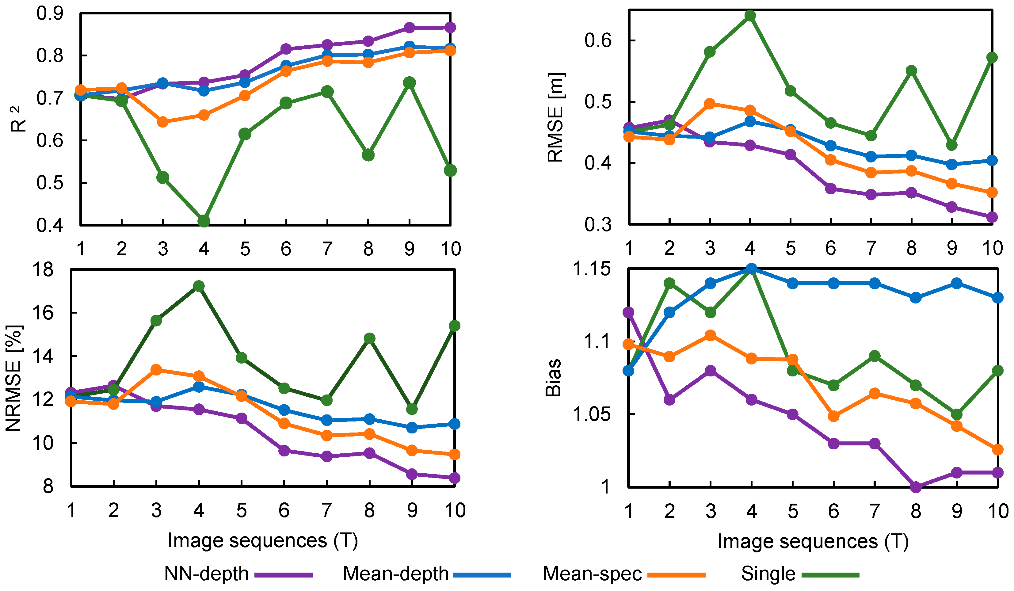
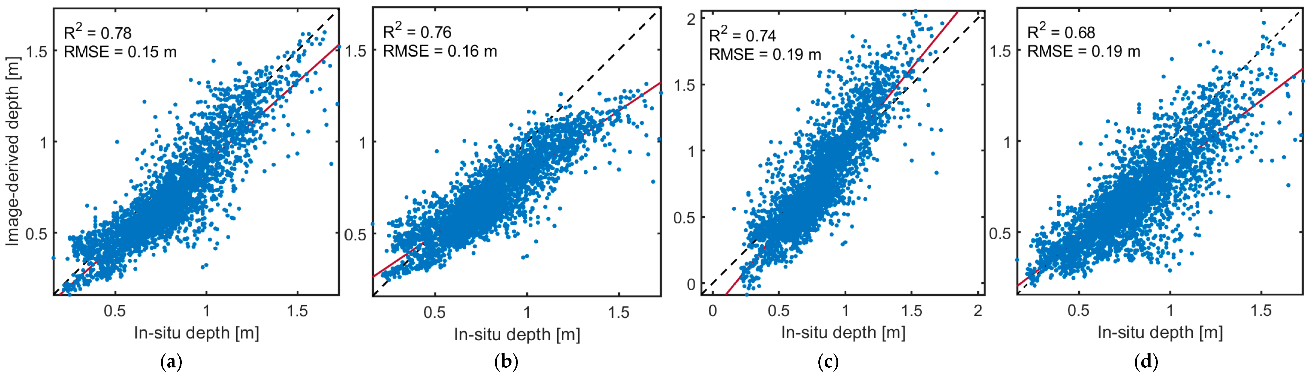
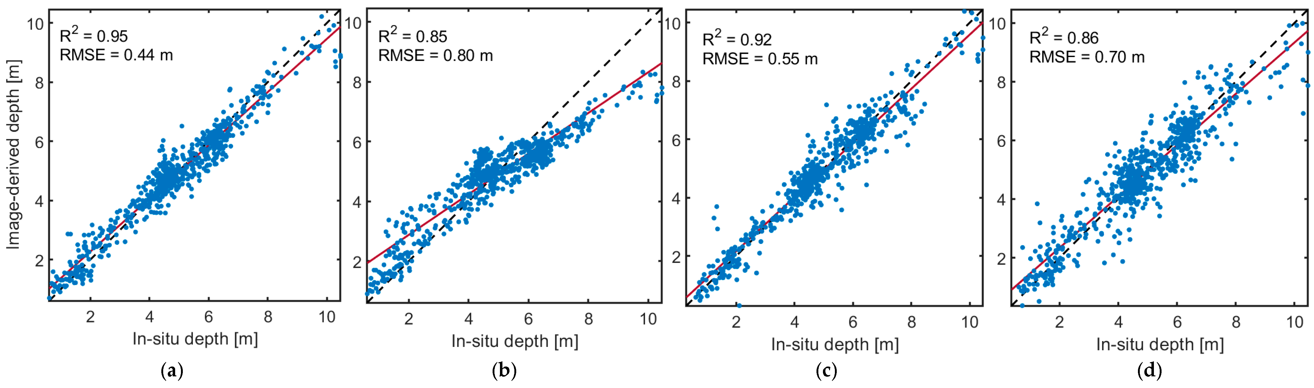
We used a set of metrics to compare the retrieved depths versus the in situ validation measurements, including the coefficient of determination (R²); root mean square error (RMSE); normalized RMSE (NRMSE), which calculates the percentage of RMSE relative to the range of water depth (max–min); and bias. Bias values close to 1 indicate that the depth estimates are subject to minimal systematic errors, whereas overestimation and underestimation lead to bias >1 and <1, respectively. For instance, a bias of 1.1 conveys that the estimated depths are 10% overestimated on average [34].

3. Case Studies and Datasets

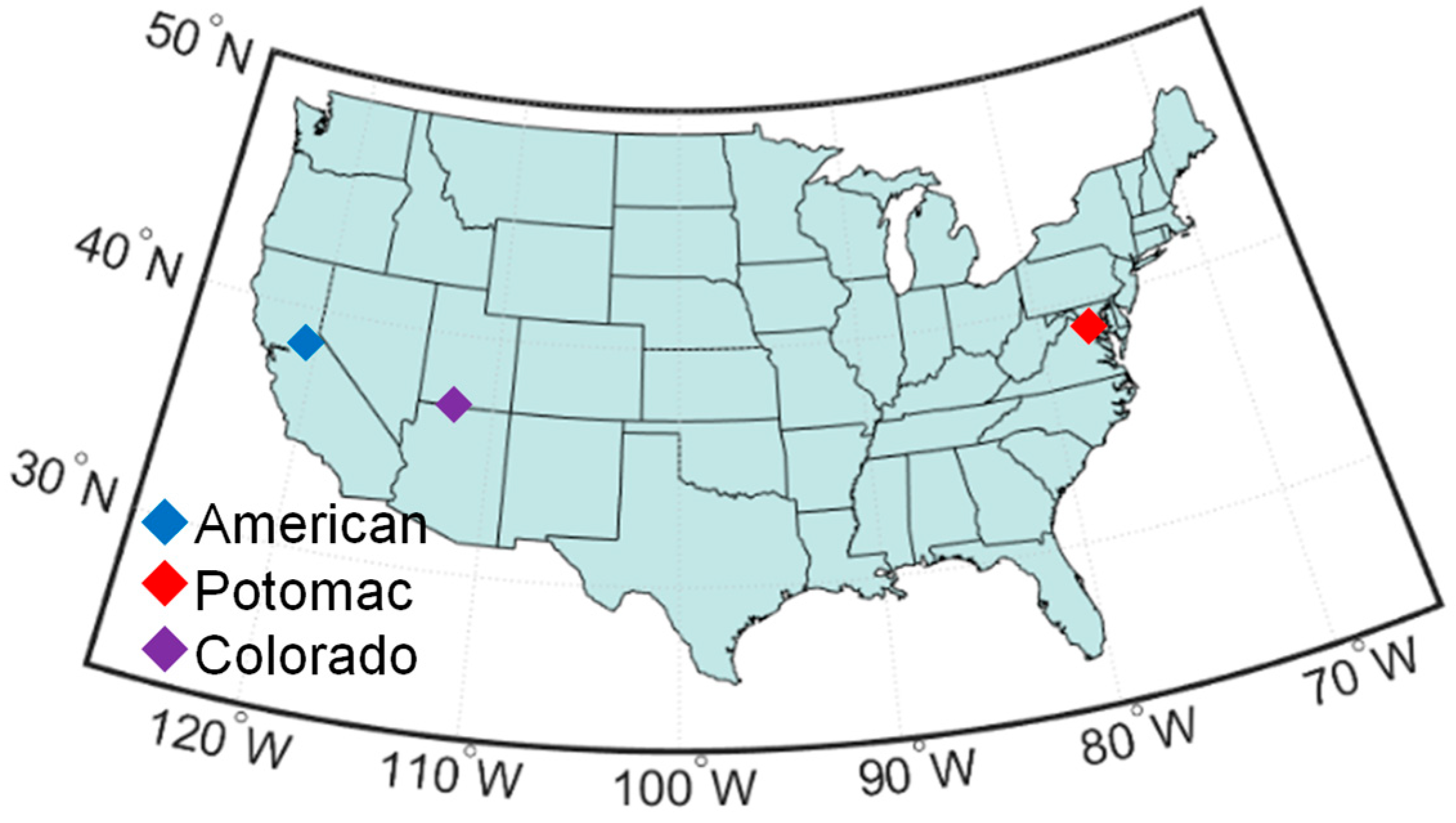
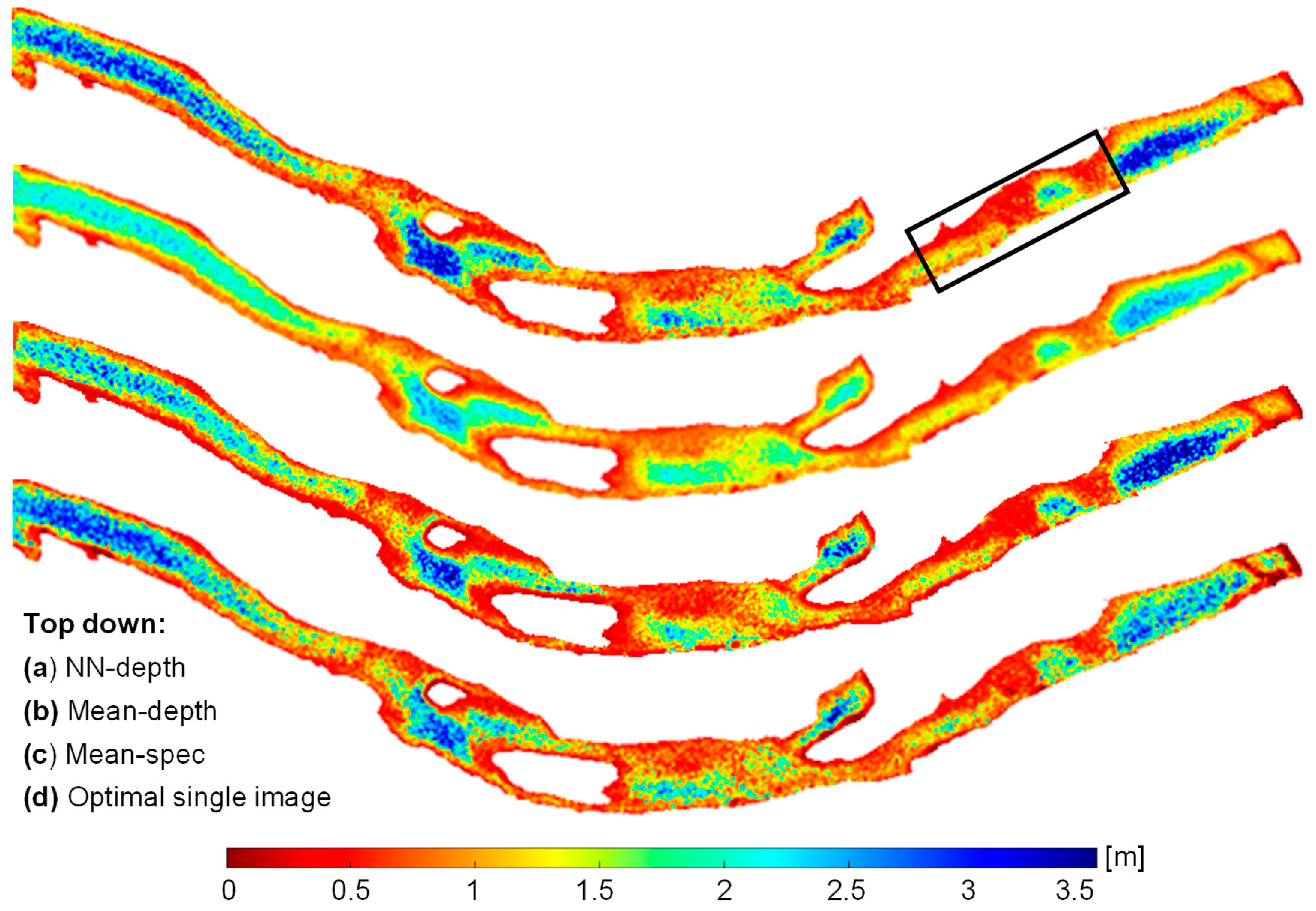
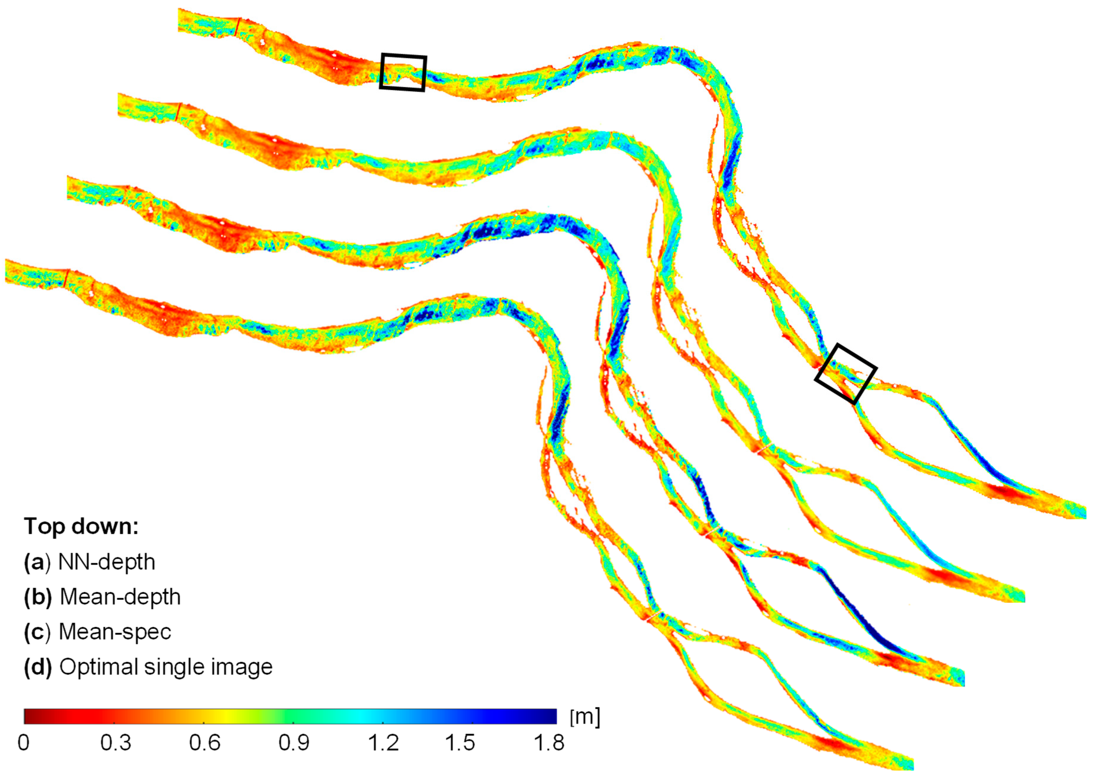
Three reaches of the American, Potomac, and Colorado rivers in the United States were studied to examine the effectiveness of different temporal ensembling methods in retrieving bathymetry (Figure 3). The study sites represent clear waters suitable for spectrally based bathymetry retrieval. However, the river reaches differ regarding the range of water depths. The Potomac reach involves very shallow waters up to a maximum of ~2 m. Although the bottom-reflected signal (i.e., the radiance component of interest for bathymetry) is pronounced in such a shallow setting, the variations in bottom type can pose challenges to depth retrieval. The American site represents deeper waters of up to ~3.5 m, whereas the Colorado reach includes waters with ~10 m depths. Thus, the selected sites permit a thorough assessment of the proposed NN–depth ensembling on clear waters.

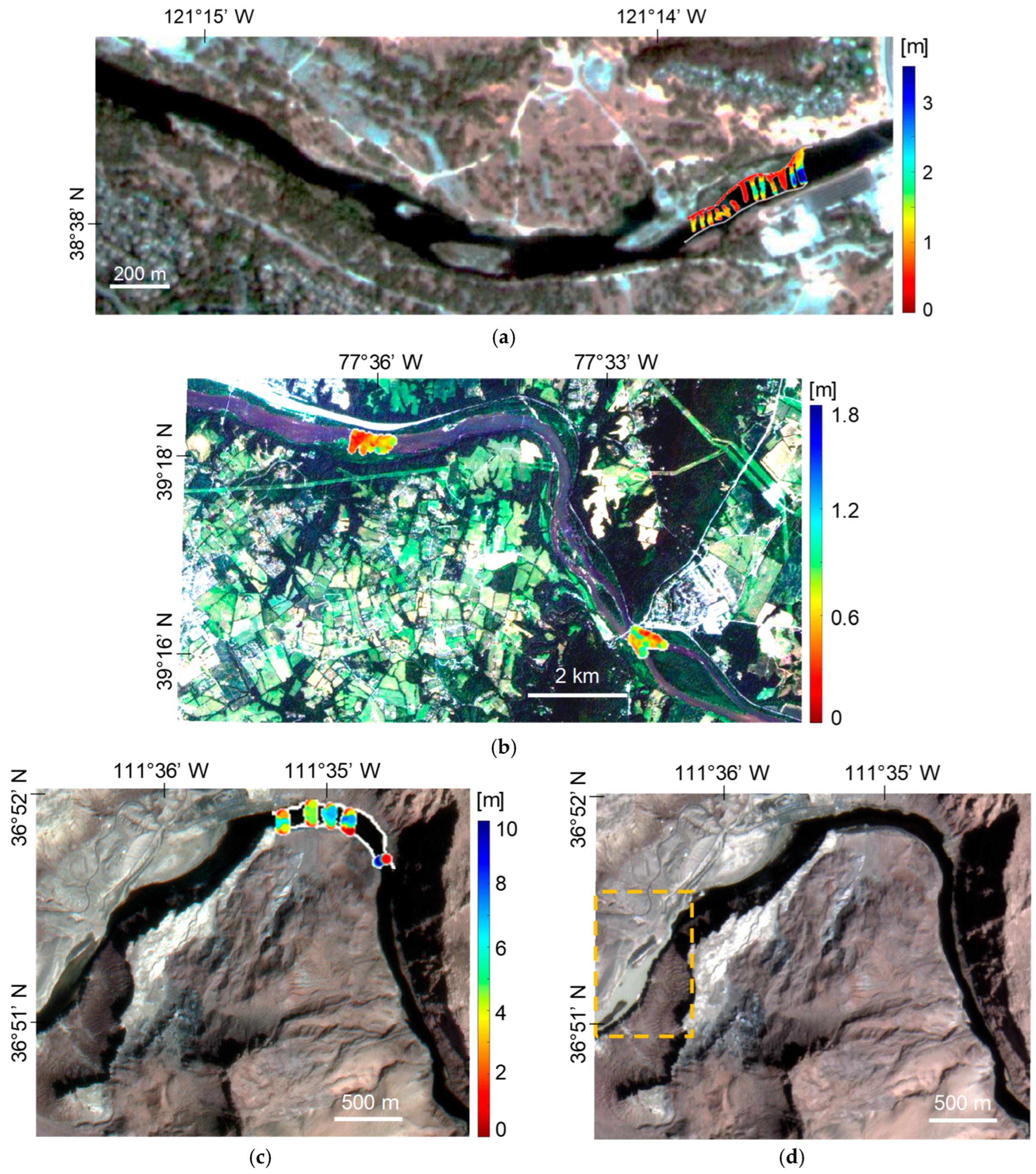
We employed in situ bathymetry data collected previously in each river for training and validation of the depth retrieval models. Figure 4 shows the in situ data superimposed on the SuperDove imagery of the study sites. Since the in situ data are collected with a spatial resolution to the order of a few centimeters, all depth measurements within each pixel were averaged to align with the spectral data at the resolution of an image pixel. The high density of field measurements ensured that this approach would provide representative pixel-scale mean depths. The field data and the details of the measurements can be found in the U.S. Geological Survey (USGS) data releases [35,36,37]. In the cases of the American and Colorado rivers, half of the in situ samples were used for training, and the second half was held out for validation (

Table 1. Summary of image and field data for each river studied.

River	Number of Images	Image Acquisition Period	Number of Field Samples	In Situ Min–Max Depth [m]	Discharge Range [m3/s]	M ± SD of RMSE for Tie Points [m]
American	10	10−30 October 2020	1274	0.03−3.75	47.5−46.7	2.3 ± 0.15
Potomac	11	23 July−13 August 2021	5199	0.14−2.11	62−58	1.9 ± 0.1
Colorado	35	1 March−11 April 2021	1342	0.54−10.45	325−319	1.6 ± 0.1

). The field survey in the Potomac River covers two distinct reaches (Figure 4b). Thus, we considered the northern reach for training (1715 samples) and the other for validation (3484 samples).

A set of temporal SuperDove images was downloaded for each river, including 10, 11, and 35 images for the American, Potomac, and Colorado, respectively. A tributary, called the Paria River, feeds into the Colorado River and can introduce significant sediment during flash floods. One of the images from Colorado, acquired at time instance 10 (T10), captured a sediment plume introduced by the Paria River in the western part of the studied reach. The area affected by the sediment plume is not within the area surveyed in the field, however. Thus, the plume did not affect the training and validation of the models. However, this image can provide insight into the robustness of different ensembling approaches when extending the depth retrieval to larger reaches in the presence of such environmental perturbations. Thus, the T10 image from the Colorado River was included in our analysis to evaluate the behavior of different ensembling approaches. The images acquired before and during the flood are shown in Figure 4c and 4d, respectively.

In this study, we employed all eight bands (443 to 865 nm) of SuperDove imagery. However, the surface reflectance products of Planet are not suitable for aquatic applications, and they provide unrealistic spectral shapes and large temporal inconsistencies over water bodies, particularly shallow rivers [12,27]. Thus, we employed the TOA radiance data by converting them to TOA reflectance using image-specific coefficients provided in the metadata. The radiance-to-reflectance conversion minimizes the effect of temporal variations in sensor viewing and solar illumination geometries. The selected images are cloud-free and represent similar discharges relative to the condition during in situ data acquisition. The USGS gage records were used to identify the dates with similar discharges (Table 1). A visual inspection of in situ data superimposed on the SuperDove imagery (Figure 4) indicated that the field data fall within the wetted channel, as depicted in the images. To quantify the geolocational accuracy of the imagery, we used very-high-resolution (0.6 m) aerial imagery from the National Agricultural Imagery Program (NAIP) [38] to select reference points. Corresponding points on the SuperDove imagery were then identified to build a set of tie points. For each study site, we extracted the spatial coordinates of 20 tie points, focusing on distinct features that were easily recognizable in both aerial and SuperDove images, such as road intersections, building corners, or other landmarks. Then, the RMSE for each tie point was calculated using the spatial coordinates. The average RMSE value was then computed to quantify the absolute geolocational accuracy of an image. This process was repeated for all the temporal imagery of a given study site using the same reference points derived from the aerial image. After calculating an average RMSE for each SuperDove image, the average (M) and standard deviation (SD) of the RMSEs were calculated for the temporal imagery of each site (Table 1). The SD of the RMSEs served as an indicator for the temporal stability of the SuperDove imagery in terms of its geolocational accuracy. These analyses indicated sub-pixel absolute geometric accuracy for all the study sites considering the SuperDove imagery with a 3 m spatial resolution. Moreover, the SD was very small (0.1 m), indicating high temporal stability of the imagery. This result aligns with findings from a recent study [39]. The high temporal stability of the geolocational accuracy of the imagery implies that these data are well suited for our temporal ensembling depth retrieval model.

4. Experimental Results

This section compares the results of various temporal ensembling methods for each river, along with single-image analysis results.

4.1. American River

The proposed NN–depth ensembling of temporal imagery provides improved depth retrieval in the American River (Figure 5). For instance, the R² improves from 0.81 to 0.87 using NN–depth instead of mean–spec ensembling. As indicated in Figure 5b,c, the mean–depth and mean–spec ensembling approaches lead to underestimates in deeper water (>2 m). This finding can be attributed to the lower signal-to-noise ratio (SNR) in deeper parts of the channel where most of the incident solar radiation is attenuated within the water column, leaving relatively little energy to be reflected toward the sensor. The image at time instance 9 (T9) provided the optimal depth retrieval for single-image analysis. However, the depth estimates based on standard single-image analysis are less accurate than all ensembling approaches, indicating the value of leveraging temporal data. The results shown in Figure 5 are based on ensembling all temporal data from the American River (10 images). We also evaluate the performance of different ensembling approaches in terms of the number of images involved. In Figure 6, the accuracy metrics are calculated based on all the images acquired prior to and including the time instance T in the temporal ensembling. The performance of the proposed NN–depth ensembling improves all the accuracy metrics by increasing the number of images. The mean–spec ensembling also benefits from an increased number of images. However, the trend lines of accuracy metrics for the NN–depth approach show fewer fluctuations than that of mean–spec, implying that NN–depth ensembling is more robust. Thus, the performance of the proposed NN–depth ensembling improves or remains steady when the depth estimates from individual bathymetry models are incorporated as new features. (e.g., the accuracy of mean–spec ensembling drops when the T3 image is included, whereas NN–depth remains more robust).

The depth retrieval based on single-image analysis shows relatively high fluctuations, with R² between 0.4 (T4) and 0.73 (T9) (Figure 6). The temporal inconsistencies of single-image analysis can be attributed to several factors, including variations in atmospheric conditions and surface glint. Any possible radiometric inconsistencies among SuperDove sensors can also affect the performance of bathymetry retrieval based on single-image analysis. Although the water constituents (e.g., suspended sediments) are expected to show less variability during a steady discharge condition, small variations can introduce uncertainties to depth retrieval. Thus, variations in optically significant water column constituents over time might account for some of the inconsistency in the single-image analysis.

The bathymetry maps derived from different ensembling methods are presented in Figure 7, along with the map derived from the optimal single-image analysis (time instance with the highest accuracy). The proposed NN–depth ensembling yields a better representation of the hydro-morphological units. For instance, the pools are captured more effectively. Although the mean–depth ensembling yielded a smooth depth map, it significantly underestimates the deep waters. The unreliable estimates of the mean–depth approach for deep waters are also evident on the validation scatterplot (Figure 5b).

4.2. Potomac River

The proposed NN–depth ensembling provided slightly improved depth retrieval relative to other approaches on the Potomac River. The NN–depth improvement is more notable compared to mean–spec ensembling and single-image analysis (Figure 8).

Figure 9 illustrates the trends of accuracy metrics by increasing the number of temporal images involved in the ensembling. Similar to the American River analysis, the accuracy metrics for the proposed NN–depth ensembling tend to improve or remain steady by incorporating more images. The mean–spec approach shows slight fluctuations in the accuracy metrics, whereas the variations are more pronounced for the single-image analysis. Figure 10 illustrates the bathymetry maps derived from various methods. The most notable differences between the maps are associated with the mean–depth approach, which yields underestimates in deep waters. This result is a consequence of the underestimates evident in Figure 8b for water deeper than ~1 m. However, the proposed NN–depth method provides accurate and consistent depth estimates across the full range of depths present within the river.

4.3. Colorado River

The NN–depth ensembling approach outperforms other models in the Colorado River, with an R² = 0.95 and an RMSE of 0.44 m for retrieving depths of up to 10 m (Figure 11). Similar to the other case studies, mean–depth ensembling suffers from underestimating the deeper waters (depth > 6 m). The depth retrieval accuracy metrics for the Colorado River are illustrated in Figure 12, which evaluates the effect of the number of images involved in the temporal ensembling. Again, all the metrics improve as the number of images increases. The bias for the NN–depth approach shows slight fluctuations, but the biases are very small (values very close to 1). The variations in the accuracy metrics over time are notable for the single-image analysis. Similar to other case studies, these temporal inconsistencies can be attributed to the variations in water surface sun glint, atmospheric effects, and radiometric quality of the imagery.

The bathymetry maps derived from different ensembling approaches as well as the optimal single-image analysis are shown in Figure 13. Although the validation of different ensembling approaches (Figure 11 and Figure 12) was not affected by the image that included a sediment plume (acquired at T10; Figure 4d), the bathymetry maps convey more information about the performance of models in this area. The mean–spec approach is affected the most in the sediment plume region (shown by a box in Figure 13c). The depth estimates are negative in this area, implying the high sensitivity of the mean–spec ensembling to confounding factors like water turbidity. This is because the spectra for turbid waters are quite different from those for clear water, leading to distortion of the time-averaged spectra. Depth retrieval in very turbid waters is not feasible based on spectrally based methods [40], and one could simply remove the T10 image from the analysis. However, this experiment provides more insight into the performance of different models when the images to which the models are applied include some artifacts (turbidity, glint, etc.). The depth estimates based on the proposed NN–depth ensembling in the sediment plume region are reliable and comparable with the range of depths derived from the optimal single image (T26). The image acquired at T26 is far removed from the flooding event and represents clear water across the studied reach. Given that the range of depths derived from NN–depth ensembling in the region affected by the sediment plume is comparable with that of the single-image analysis (T26), this indicates that the proposed NN–depth ensembling is robust in the presence of confounding effects like turbidity. Similar to other case studies, the depths based on the mean–depth ensembling are smoothed out, leading to underestimation in deeper parts of the channel. This finding aligns with the validation scatterplot (Figure 11b), indicating the underestimation problem.

The depth maps presented in Figure 13 are based on the temporal ensembling of all 35 images from the Colorado River. Figure 14 shows the bathymetric maps by ensembling all the imagery acquired before (T1 to T9) and right after (T1 to T10) the flood event. The maps are illustrated for the proposed NN–depth compared to the mean–spec ensembling. This experiment indicates that the proposed NN–depth ensembling remains relatively robust right after introducing the image affected by the sediment plume (T10), although some details are smoothed out. The depth map involving all 35 images through NN–depth ensembling (Figure 13a) is more comparable with the before-flood map in the flooded region (Figure 14a). This finding indicates that incorporating more images through the NN–depth ensembling can enhance the robustness of the model in the presence of confounding effects like turbidity. However, the problem on the bathymetric map of the mean–spec ensembling approach right after the flooding event (Figure 14d) is as severe as when incorporating all 35 images (Figure 13c). The depth estimates on both maps are mainly negative values. This finding shows that incorporating a single image affected by turbid waters through mean–spec ensembling can lead to unreliable depth estimates even when the ensembling incorporates a considerable number (35) of temporal images.

Increasing the number of images will not necessarily enhance depth retrieval via the proposed NN–depth ensembling, but this approach does increase the likelihood of obtaining images of high radiometric quality (e.g., favorable illumination and atmospheric conditions, minimal sun glint artifacts) throughout the time series, regardless of the number of images. The acquisition of imagery conducive to depth retrieval depends on various factors (e.g., acquisition period) and enhances the predictive power of the ensemble model. This improvement is evident in the accuracy trendline for the Colorado River (Figure 12), where incorporating imagery at time instances 25 and 26 significantly improves depth retrieval (improvements in R² and RMSE of approximately 0.05 and 0.2 m, respectively). Although the Colorado River benefits from a higher number of images than the American and Potomac rivers, depth retrievals based on individual images are also more accurate than for the other two rivers. For instance, the average R² of single-image depth retrievals is 0.69 for the Colorado River, compared to 0.61 and 0.56 for the American and Potomac rivers, respectively. This result can be attributed to the deeper water in the Colorado River, which mitigates the confounding effects of bottom-type variability and sun glint artifacts that are often more pronounced in shallow river settings.

5. Discussion

This study introduced a new approach for ensembling the dense time-series imagery provided by SuperDove CubeSats to improve bathymetry retrieval in optically shallow waters. The proposed NN–depth ensembling performs the fusion at the product level (bathymetry maps) rather than the data level (time series of images). The performance of depth retrieval from single-image analysis varies due to factors such as sun glint, atmospheric conditions, CubeSat radiometric inconsistencies, and variations in water column optical properties. However, because the proposed model treats the images individually at the first stage (i.e., depth retrieval), it mitigates against the propagation of spectral uncertainties through the ensembling. In contrast, the time-averaged image derived from the first stage of the mean–spec ensembling is affected by any kind of environmental and/or instrumental noise present in any of the individual images. Given that confounding factors like sun glint and water turbidity are variable over both space and time, the relative consistency of the spectra among different pixels can be degraded by time-averaging the spectra. The inconsistencies can be larger when the temporal imagery spans a longer period, which might encompass variations in atmospheric effects that also introduce challenges to the mean–depth ensembling approach. Moreover, the proposed NN–depth ensembling essentially learns the relationships between depths derived at different time instances and the reference depths measured in the field. This machine learning mechanism for ensembling the temporal depths automatically defines each time instance’s contribution to the final depth estimates. Therefore, the performance of the proposed NN–depth ensembling either improves or remains consistent when the depth estimates from individual bathymetry models are integrated as new features. Furthermore, ensembling at the product level (water depths) can also serve as an error compensation, as the model has the chance to essentially remap the depths derived from individual images to the field-based reference depths. The high accuracies achieved based on independent in situ data (Section 3) imply that the proposed ensemble model is not overfitted and demonstrates its strong predictive capability. On the other hand, the mean–depth ensembling assumes an equal contribution for the depth estimates at individual time instances to drive the final bathymetry estimate. Thus, this approach lacks the advantages of the NN–depth model in terms of weighting the time instances and compensating for errors.

6. Conclusions and Future Outlook

In this study, we proposed a machine learning approach to enhance bathymetry retrieval from time-series imagery. The new method presented herein involves ensembling water depths derived from individual images rather than ensembling the spectral data first and then proceeding to depth retrieval. The proposed NN–depth ensembling provided more accurate and robust retrievals of bathymetry relative to other approaches, including mean–spec and mean–depth ensembling models. Given the reduced sensitivity of the NN–depth ensembling to variations in the confounding factors over time, this ensembling approach can benefit from temporal imagery spanning a relatively long period, provided the bathymetry remains steady. The robust behavior of the NN–depth ensembling would be particularly valuable in an operational monitoring context in which images are processed as they are acquired, without any automatic means of accounting for episodic perturbations such as a sediment plume. In addition, this study provided further evidence of the utility of the newly available SuperDove imagery in bathymetric applications, as initially demonstrated in a comparative study with Landsat-9 and Sentinel-2A/B [27].

Similar to other empirical bathymetric models, the proposed bathymetry method is constrained by the availability of in situ data. However, the in situ data required for training NN–depth ensembling does not need to be a lengthy time series; in fact, only field data from a single time instance are required. This approach is predicated upon the assumption that the images are acquired under steady flow conditions. Thus, the required field data are minimal and equivalent to those needed for the analysis of a single image. Moreover, since shallow neural networks are utilized, the number of training samples does not need to be unusually large. Although we performed the bathymetry retrieval in rivers, the proposed methodology is generic and can be applied to any optically shallow environment. This study leveraged NNs to ensemble the temporal depths. Future studies could be devoted to evaluating other machine/deep learning models, like decision trees, support vector machines, and convolutional NNs. In this study, we used automatic hyperparameter tuning to define the structure of the NNs through the proposed ensembling. However, we also demonstrated that a simple, fixed architecture can be used in cases where the training and prediction are applied to individual images [12]. Applying a common, fixed architecture to process multitemporal data can facilitate routine application of the proposed method. In this study, we used TOA data, as Planet’s standard surface reflectance products are not useful for aquatic applications. The dark spectrum fitting (DSF) atmospheric correction and the exponential model implemented in the ACOLITE processor are the only aquatic-specific atmospheric corrections that can currently be applied to SuperDove imagery [11,41]. However, these methods are mainly suitable for turbid waters [42,43], which is not the case for bathymetric applications. The effect of atmospheric correction on the performance of the ensembling approaches can be investigated as more methods become available. However, this effect is expected to be minimal for the proposed NN–depth ensembling because the approach treats every image individually at the first stage, and regression-based depth retrieval on a single image can achieve even better results using TOA rather than BOA, particularly when the atmospheric correction is not reliable [12]. However, mean–spec ensembling can benefit from an accurate atmospheric correction, as it can enhance the consistency among temporal images and, thus, the quality of the time-averaged image. In the future, the acquisition of CubeSat images will become even more frequent, with up to 30 images captured each day, as a result of a new Planet mission called Pelican [44]. The novel approach to ensembling described herein will provide an effective means of incorporating the temporally rich data from this new constellation to produce accurate, highly robust bathymetric data products. Notably, the proposed NN–depth ensembling approach is not limited to CubeSat data and could also be applied to time-series imagery from other satellite or airborne missions.

References

1. Roy, D.P.; Huang, H.; Houborg, R.; Martins, V.S. A Global Analysis of the Temporal Availability of Planet Scope High Spatial Resolution Multi-Spectral Imagery. Remote Sens. Environ. 2021, 264, 112586. [Google Scholar] [CrossRef]
2. Planet Team Planet Imagery Product Specifications. Available online: https://www.planet.com/products/ (accessed on 5 January 2021).
3. Tu, Y.-H.; Johansen, K.; Aragon, B.; El Hajj, M.M.; McCabe, M.F. The Radiometric Accuracy of the 8-Band Multi-Spectral Surface Reflectance from the Planet SuperDove Constellation. Int. J. Appl. Earth Obs. Geoinf. 2022, 114, 103035. [Google Scholar] [CrossRef]
4. Kääb, A.; Altena, B.; Mascaro, J. River-Ice and Water Velocities Using the Planet Optical Cubesat Constellation. Hydrol. Earth Syst. Sci. 2019, 23, 4233–4247. [Google Scholar] [CrossRef]
5. Kerr, J.M.; Purkis, S. An Algorithm for Optically-Deriving Water Depth from Multispectral Imagery in Coral Reef Landscapes in the Absence of Ground-Truth Data. Remote Sens. Environ. 2018, 210, 307–324. [Google Scholar] [CrossRef]
6. Jorge, D.S.F.; Barbosa, C.C.F.; De Carvalho, L.A.S.; Affonso, A.G.; Lobo, F.D.L.; Novo, E.M.L.D.M. SNR (Signal-To-Noise Ratio) Impact on Water Constituent Retrieval from Simulated Images of Optically Complex Amazon Lakes. Remote Sens. 2017, 9, 644. [Google Scholar] [CrossRef]
7. Brando, V.E.; Dekker, A.G. Satellite Hyperspectral Remote Sensing for Estimating Estuarine and Coastal Water Quality. IEEE Trans. Geosci. Remote Sens. 2003, 41, 1378–1387. [Google Scholar] [CrossRef]
8. Niroumand-Jadidi, M.; Bovolo, F.; Bresciani, M.; Gege, P.; Giardino, C. Water Quality Retrieval from Landsat-9 (OLI-2) Imagery and Comparison to Sentinel-2. Remote Sens. 2022, 14, 4596. [Google Scholar] [CrossRef]
9. Poursanidis, D.; Traganos, D.; Chrysoulakis, N.; Reinartz, P. Cubesats Allow High Spatiotemporal Estimates of Satellite-Derived Bathymetry. Remote Sens. 2019, 11, 1299. [Google Scholar] [CrossRef]
10. Cooley, S.; Smith, L.; Stepan, L.; Mascaro, J. Tracking Dynamic Northern Surface Water Changes with High-Frequency Planet CubeSat Imagery. Remote Sens. 2017, 9, 1306. [Google Scholar] [CrossRef]
11. Vanhellemont, Q. Daily Metre-Scale Mapping of Water Turbidity Using CubeSat Imagery. Opt. Express 2019, 27, A1372. [Google Scholar] [CrossRef]
12. Niroumand-Jadidi, M.; Legleiter, C.J.; Bovolo, F. Bathymetry Retrieval from CubeSat Image Sequences with Short Time Lags. Int. J. Appl. Earth Obs. Geoinf. 2022, 112, 102958. [Google Scholar] [CrossRef]
13. Legleiter, C.J.; Roberts, D.A. A Forward Image Model for Passive Optical Remote Sensing of River Bathymetry. Remote Sens. Environ. 2009, 113, 1025–1045. [Google Scholar] [CrossRef]
14. Casal, G.; Hedley, J.D.; Monteys, X.; Harris, P.; Cahalane, C.; McCarthy, T. Satellite-Derived Bathymetry in Optically Complex Waters Using a Model Inversion Approach and Sentinel-2 Data. Estuar. Coast. Shelf Sci. 2020, 241, 106814. [Google Scholar] [CrossRef]
15. Maciel, D.A.; Novo, E.M.L.D.M.; Barbosa, C.C.F.; Martins, V.S.; Júnior, R.F.; Oliveira, A.H.; De Carvalho, L.A.S.; Lobo, F.D.L. Evaluating the Potential of CubeSats for Remote Sensing Reflectance Retrieval over Inland Waters. Int. J. Remote Sens. 2020, 41, 2807–2817. [Google Scholar] [CrossRef]
16. Li, J.; Knapp, D.E.; Schill, S.R.; Roelfsema, C.; Phinn, S.; Silman, M.; Mascaro, J.; Asner, G.P. Adaptive Bathymetry Estimation for Shallow Coastal Waters Using Planet Dove Satellites. Remote Sens. Environ. 2019, 232, 111302. [Google Scholar] [CrossRef]
17. Mandlburger, G. A Review of Active and Passive Optical Methods in Hydrography. Int. Hydrogr. Rev. 2022, 28, 8–52. [Google Scholar] [CrossRef]
18. Lyzenga, D.R.; Malinas, N.P.; Tanis, F.J. Multispectral Bathymetry Using a Simple Physically Based Algorithm. IEEE Trans. Geosci. Remote Sens. 2006, 44, 2251–2259. [Google Scholar] [CrossRef]
19. Slocum, R.K.; Parrish, C.E.; Simpson, C.H. Combined Geometric-Radiometric and Neural Network Approach to Shallow Bathymetric Mapping with UAS Imagery. ISPRS J. Photogramm. Remote Sens. 2020, 169, 351–363. [Google Scholar] [CrossRef]
20. Niroumand-Jadidi, M.; Bovolo, F.; Bruzzone, L. SMART-SDB: Sample-Specific Multiple Band Ratio Technique for Satellite-Derived Bathymetry. Remote Sens. Environ. 2020, 251, 112091. [Google Scholar] [CrossRef]
21. Hsu, H.-J.; Huang, C.-Y.; Jasinski, M.; Li, Y.; Gao, H.; Yamanokuchi, T.; Wang, C.-G.; Chang, T.-M.; Ren, H.; Kuo, C.-Y.; et al. A Semi-Empirical Scheme for Bathymetric Mapping in Shallow Water by ICESat-2 and Sentinel-2: A Case Study in the South China Sea. ISPRS J. Photogramm. Remote Sens. 2021, 178, 1–19. [Google Scholar] [CrossRef]
22. Mobley, C.D. Light and Water: Radiative Transfer in Natural Waters; Academic Press: Cambridge, MA, USA, 1994; ISBN 9780125027502. [Google Scholar]
23. Hedley, J.; Russell, B.; Randolph, K.; Dierssen, H. A Physics-Based Method for the Remote Sensing of Seagrasses. Remote Sens. Environ. 2016, 174, 134–147. [Google Scholar] [CrossRef]
24. Eugenio, F.; Marcello, J.; Martin, J. High-Resolution Maps of Bathymetry and Benthic Habitats in Shallow-Water Environments Using Multispectral Remote Sensing Imagery. IEEE Trans. Geosci. Remote Sens. 2015, 53, 3539–3549. [Google Scholar] [CrossRef]
25. Niroumand-Jadidi, M.; Bovolo, F.; Bruzzone, L.; Gege, P. Physics-Based Bathymetry and Water Quality Retrieval Using PlanetScope Imagery: Impacts of 2020 COVID-19 Lockdown and 2019 Extreme Flood in the Venice Lagoon. Remote Sens. 2020, 12, 2381. [Google Scholar] [CrossRef]
26. Stumpf, R.P.; Holderied, K.; Sinclair, M. Determination of Water Depth with High-Resolution Satellite Imagery over Variable Bottom Types. Limnol. Ocean. 2003, 48, 547–556. [Google Scholar] [CrossRef]
27. Niroumand-Jadidi, M.; Legleiter, C.J.; Bovolo, F. River Bathymetry Retrieval From Landsat-9 Images Based on Neural Networks and Comparison to SuperDove and Sentinel-2. IEEE J. Sel. Top. Appl. Earth Obs. Remote Sens. 2022, 15, 5250–5260. [Google Scholar] [CrossRef]
28. Legleiter, C.J.; Kinzel, P.J. Improving Remotely Sensed River Bathymetry by Image-Averaging. Water Resour. Res. 2021, 57, e2020WR028795. [Google Scholar] [CrossRef]
29. Mandlburger, G.; Kölle, M.; Nübel, H.; Soergel, U. BathyNet: A Deep Neural Network for Water Depth Mapping from Multispectral Aerial Images. PFG J. Photogramm. Remote Sens. Geoinf. Sci. 2021, 89, 71–89. [Google Scholar] [CrossRef]
30. Snoek, J.; Larochelle, H.; Adams, R.P. Practical Bayesian Optimization of Machine Learning Algorithms. In Advances in Neural Information Processing Systems; Pereira, F., Burges, C.J., Bottou, L., Weinberger, K.Q., Eds.; Curran Associates, Inc.: Red Hook, NY, USA, 2012; Volume 25. [Google Scholar]
31. Gelbart, M.A.; Snoek, J.; Adams, R.P. Bayesian Optimization with Unknown Constraints. arXiv 2014, arXiv:1403.5607. [Google Scholar] [CrossRef]
32. He, K.; Zhang, X.; Ren, S.; Sun, J. Delving Deep into Rectifiers: Surpassing Human-Level Performance on ImageNet Classification. In Proceedings of the 2015 IEEE International Conference on Computer Vision (ICCV), Santiago, Chile, 7–13 December 2015. [Google Scholar]
33. MATLAB. Deep Learning Toolbox; The MathWorks Inc.: Natick, MA, USA, 2022. [Google Scholar]
34. Seegers, B.N.; Stumpf, R.P.; Schaeffer, B.A.; Loftin, K.A.; Werdell, P.J. Performance Metrics for the Assessment of Satellite Data Products: An Ocean Color Case Study. Opt. Express 2018, 26, 7404. [Google Scholar] [CrossRef]
35. Legleiter, C.J.; Harrison, L.R. Field Measurements of Water Depth from the American River near Fair Oaks, CA, October 19–21, 2020; United States Geological Survey Data Release: Reston, VA, USA, 2021. [Google Scholar] [CrossRef]
36. Duda, J.M.; Greise, A.J.; Young, J.A. Potomac River ADCP Bathymetric Survey, October 2019; United States Geological Survey Data Release: Reston, VA, USA, 2020. [Google Scholar]
37. Legleiter, C.J.; Debenedetto, G.P.; Forbes, B.T. Field Measurements of Water Depth from the Colorado River near Lees Ferry, AZ, March 16–18, 2021; United States Geological Survey Data Release: Reston, VA, USA, 2021. [Google Scholar] [CrossRef]
38. NAIP National Agricultural Imagery Program. Available online: https://earthexplorer.usgs.gov/ (accessed on 31 March 2025).
39. Semple, A.G.; Tan, B.; Lin, G. SuperDove Geometric Quality Assessment Summary; NASA: Washington, DC, USA, 2023. [Google Scholar]
40. Chen, B.; Yang, Y.; Xu, D.; Huang, E. A Dual Band Algorithm for Shallow Water Depth Retrieval from High Spatial Resolution Imagery with No Ground Truth. ISPRS J. Photogramm. Remote Sens. 2019, 151, 1–13. [Google Scholar] [CrossRef]
41. Vanhellemont, Q. Sensitivity Analysis of the Dark Spectrum Fitting Atmospheric Correction for Metre- and Decametre-Scale Satellite Imagery Using Autonomous Hyperspectral Radiometry. Opt. Express 2020, 28, 29948–29965. [Google Scholar] [CrossRef] [PubMed]
42. Vanhellemont, Q.; Ruddick, K. Atmospheric Correction of Metre-Scale Optical Satellite Data for Inland and Coastal Water Applications. Remote Sens. Environ. 2018, 216, 586–597. [Google Scholar] [CrossRef]
43. Vanhellemont, Q.; Ruddick, K. Atmospheric Correction of Sentinel-3/OLCI Data for Mapping of Suspended Particulate Matter and Chlorophyll-a Concentration in Belgian Turbid Coastal Waters. Remote Sens. Environ. 2021, 256, 112284. [Google Scholar] [CrossRef]
44. Planet Pelican|Planet. Available online: https://www.planet.com/products/pelican/ (accessed on 1 July 2022).
45. Legleiter, C.J.; Niroumand-Jadidi, M. Maps of Water Depth Derived from Satellite Images of Selected Reaches of the American, Colorado, and Potomac Rivers Acquired in 2020 and 2021 (Ver. 2.0, September 2024); United States Geological Survey Data Release: Reston, VA, USA, 2024. [Google Scholar] [CrossRef]
Figure 1. A schematic representation of the neural network-based depth retrieval (NNDR) architecture. The layer sizes are simplified for visualization purposes.
Remotesensing 17 01309 g001
Figure 2. The workflow of the proposed neural net regressor (NN–depth) ensembling method for retrieving bathymetry from temporally dense SuperDove imagery, along with the mean–spec and mean–depth approaches.
Remotesensing 17 01309 g002
Figure 3. Location of the studied reaches in the American, Potomac and Colorado rivers. The extents of each river reach are shown in Figure 4.
Remotesensing 17 01309 g003
Figure 4. SuperDove imagery of (a) the American River at time instance 1 (T1), (b) the Potomac River at time instance 1 (T1), and the Colorado River (c) before (13 March 2021, time instance 9 (T9)), and (d) during the sediment plume (17 March 2021, time instance 10 (T10)). A yellow box shows the segment of the river affected by sediment. The distribution and depths of in situ samples are shown on the images.
Remotesensing 17 01309 g004
Figure 5. Validation scatterplots (in situ vs. image-derived depths) comparing the performance of bathymetry retrieval in the American River based on (a) the proposed NN–depth ensembling, (b) mean–depth ensembling, (c) mean–spec ensembling of imagery acquired from time instance 1 (T1) to T10, and (d) optimal single-image (T9) analysis. RMSE is root mean square error. The regression line is shown in red, with the dashed black line indicating the 1:1 reference.
Remotesensing 17 01309 g005
Figure 6. Accuracy statistics comparing the performance of bathymetry retrieval in the American River based on the proposed NN–depth ensembling, mean–depth ensembling, mean–spec ensembling, and optimal single-image analyses. The results for ensembling approaches at each image sequence represent the results derived from combining all the images acquired until that time instance. Root mean square error (RMSE); normalized RMSE (NRMSE).
Remotesensing 17 01309 g006
Figure 7. Bathymetry maps derived from temporal SuperDove imagery in the American River based on (a) the proposed NN–depth ensembling, (b) mean–depth ensembling, (c) mean–spec ensembling of imagery acquired from time instance 1 (T1) to T10, and (d) optimal single-image (T9) analysis. The box in (a) shows the location of in situ data.
Remotesensing 17 01309 g007
Figure 8. Validation scatterplots (in situ vs. image-derived depths) comparing the performance of bathymetry retrieval in the Potomac River based on (a) the proposed NN–depth ensembling, (b) mean–depth ensembling, (c) mean–spec ensembling of imagery acquired from T1 to T11, and (d) optimal single-image (T2) analysis. RMSE is root mean square error. The regression line is shown in red, with the dashed black line indicating the 1:1 reference.
Remotesensing 17 01309 g008
Figure 9. Accuracy statistics comparing the performance of bathymetry retrieval in the Potomac River based on the proposed NN–depth ensembling, mean–depth ensembling, mean–spec ensembling, and optimal single-image analysis. The results for the ensembling approaches at each image sequence represent the results derived from combining all the images acquired until that time instance. Root mean square error (RMSE); normalized RMSE (NRMSE).
Remotesensing 17 01309 g009
Figure 10. Bathymetry maps derived from temporal SuperDove imagery in the Potomac River based on (a) the proposed NN–depth ensembling, (b) mean–depth ensembling, (c) mean–spec ensembling of imagery acquired from time instance 1 (T1) to T11, and (d) optimal single-image (T2) analysis. The boxes in (a) show the locations of in situ data.
Remotesensing 17 01309 g010
Figure 11. Validation scatterplots (in situ vs. image-derived depths) comparing the performance of bathymetry retrieval in the Colorado River based on (a) the proposed NN–depth ensembling, (b) mean–depth ensembling, (c) mean–spec ensembling of imagery acquired from time instance 1 (T1) to T35, and (d) optimal single-image (T26) analysis. RMSE is root mean square error. The regression line is shown in red, with the dashed black line indicating the 1:1 reference.
Remotesensing 17 01309 g011
Figure 12. Accuracy statistics comparing the performance of bathymetry retrieval in the Colorado River based on the proposed NN–depth ensembling, mean–depth ensembling, mean–spec ensembling, and optimal single-image analyses. The results for ensembling approaches at each image sequence represent the results derived from combining all the images acquired until that time instance. Root mean square error (RMSE); normalized RMSE (NRMSE).
Remotesensing 17 01309 g012
Figure 13. Bathymetry maps derived from temporal SuperDove imagery in the Colorado River based on (a) the proposed NN–depth ensembling, (b) mean–depth ensembling, (c) mean–spec ensembling of imagery acquired from time instance 1 (T1) to T35, and (d) optimal single-image (T26) analysis. The dashed rectangle shows the area affected by the sediment plume. The box in (c) shows the location of in situ data.
Remotesensing 17 01309 g013
Figure 14. Bathymetry maps derived from SuperDove imagery in the Colorado River by performing the temporal ensembling prior to (time instance 1 (T1) to T9) and right after (T1 to T10) the flooding event based on the NN–depth and mean–spec ensembling methods.
Remotesensing 17 01309 g014