Analysis and Modeling of Statistical Distribution Characteristics for Multi-Aspect SAR Images

Abstract

Multi-aspect synthetic aperture radar (SAR) is an emerging observation mode in SAR. Through multi-aspect observations, along with coherent and incoherent image processing, multi-aspect SAR effectively addresses issues like layovers, shadows, and foreshortening in conventional SAR. It can obtain multi-aspect scattering images of the observed scene. Modeling the statistical distribution characteristics of multi-aspect SAR images is crucial for its processing and applications. Currently, there is no comprehensive and systematic study on the statistical distribution characteristics of multi-aspect SAR images. Therefore, this paper conducts qualitative and quantitative analyses of these characteristics. Furthermore, we investigate the applicability and limitations of five single-parametric models commonly used in conventional SAR for modeling the statistical distribution characteristics of multi-aspect SAR images. The experimental results show that none of these models could accurately model the multi-aspect SAR images. To address this issue, we propose a finite mixture model (FMM) and evaluate its feasibility to accurately model the statistical distribution characteristics of multi-aspect SAR on X-band GOTCHA data and C-band Zhuhai data. The experimental results demonstrate that, compared with the single-parametric models, our method can accurately model the statistical distribution characteristics of various types of targets in multi-aspect SAR images from different observation aspects and aperture angles in various bands.

1. Introduction

Synthetic aperture radar (SAR) is an active remote sensing radar that can work all-day and all-weather [1]. Conventionally, the observation mode of SAR involves observing the scene by a linear trajectory flight. However, there are two problems with this observation mode, as follows: On the one hand, conventional SAR has inherent problems, such as layovers, shadows, and foreshortening. On the other hand, it can only obtain the backscattering of the observed object from a small observation aspect. In order to meet the need for refined observations, a novel observation mode, multi-aspect SAR, is proposed [2]. Multi-aspect SAR utilizes the radar platform to conduct azimuthal observations of scenes from different aspects [3,4]. Compared with conventional SAR, multi-aspect SAR has 3D imaging capabilities. Therefore, it can reduce issues such as layovers, shadows, and foreshortening found in conventional SAR. Multi-aspect SAR can obtain backscattering data from many observation aspects. Thus, multi-aspect SAR can obtain information that is difficult to acquire with conventional SAR and provide a more comprehensive contour structure compared with conventional SAR [2]. This allows for a detailed description and analysis of an observed object.

Accurately modeling the statistical information in SAR images is crucial for its processing and application [5,6]. In the field of change detection, accurate modeling of the statistical distribution characteristics of both the change and no-change classes can significantly enhance the performance of the change detectors [7]. In the field of target detection, the effectiveness of many target detectors is highly dependent on the modeling accuracy of the clutter. Consequently, effective modeling of the clutter can improve target detection capabilities [8]. In SAR image classification, it is necessary to accurately model the statistical distribution characteristics of SAR images, which are then classified correctly according to their statistical properties [9]. In research on moving target detection, accurate modeling of background clutter is essential to improve the detection performance on moving targets [10]. These works focus on conventional SAR and employ modeling of the statistical information in the processing and application of SAR images. In fact, accurate modeling of the statistical information of multi-aspect SAR images can also enhance its processing and applications. Specifically, high-accuracy modeling of multi-aspect SAR images provides theoretical support for understanding the statistical distribution characteristics of multi-aspect SAR images and for further leveraging the advantages of detailed descriptions. However, when conducting research on the statistical distribution characteristics of multi-aspect SAR, there are two essential questions that should be explored and answered, as follows:

Q1.  

What features do the statistical distribution characteristics of multi-aspect SAR images possess?

Q2.  

Is there a model that can accurately describehe statistical distribution characteristics of multi-aspect SAR images?

In recent years, many statistical modeling methods have been proposed for analyzing the probability density function (PDF) of conventional SAR image amplitude or intensity [11,12,13]. Based on whether they have analytical expressions, as well as their complexity, SAR image statistical models can be categorized into the following three types [6]: nonparametric, parametric, and semiparametric approaches. Nonparametric models do not make assumptions about the unknown PDF of the data and can flexibly model the data [5,11]. However, they require a large number of training samples and involve heavy computation. Nonparametric methods include the Parzen window [14], artificial neural networks [15], and support vector machines [16]. Parametric methods assume a mathematical formula for each PDF and formalize the PDF-estimation problem as a parameter estimation problem [5,13]. These methods can describe the statistical distribution characteristics of data with very few parameters. However, these models are only effective for specific terrain types (e.g., urban area, forest, and water area), and they have difficulty in accurately modeling the statistical distribution characteristics of complex scenes in high-resolution SAR images containing multiple terrain types [5,13,17,18]. Parametric models include the Gamma distribution [19], Log-normal distribution [20], Weibull distribution [21], K distribution [22], and G0 distribution [23]. However, these studies focus on conventional SAR images rather than multi-aspect SAR. To address the lack of such studies on multi-aspect SAR images, we conducted a series of analyses on the statistical distribution characteristics of multi-aspect SAR images using parametric models (in view of their simplicity), exploring the applicability and limitations of these models (Q1).

After exploring the statistical distribution characteristics of multi-aspect SAR images, the subsequent question raised is whether any models exist that can accurately model them. Multi-aspect SAR images involve large volumes of data and complex terrain types, and from different aspects, the target may exhibit varying statistical distribution characteristics. Parametric models are only accurate for specific terrain types, while nonparametric models are computationally intensive and time-consuming. Therefore, neither parametric nor nonparametric models can accurately model the statistical distribution characteristics of multi-aspect SAR images. Thus, it is necessary to explore the feasibility of accurately and efficiently modeling the multi-aspect SAR. Semiparametric models combine elements of parametric models and nonparametric models and merge some advantages of both. Therefore, they can model the PDF of different data flexibly and accurately with very little increase in the computational complexity. Among semiparametric models, the finite mixture model (FMM) is a flexible and probabilistic modeling tool for univariate and multivariate data [24]. It has been successfully applied in pattern recognition, signal and image analysis, machine learning and remote sensing [18,24]. When analyzing the statistical distribution characteristics of SAR images, the FMM models the unknown PDF as a linear combination of single-parametric models [5,13,25,26]. The FMM increases the number of variables, enhancing the flexibility and capacity of the mixture model to represent the statistical distribution characteristics of high-resolution SAR images.

Recently, some studies have applied FMM to model and analyze high-resolution SAR images containing various terrain types, yielding promising results. Blake et al. proposed K-mixture distributions and Log-normal-mixture distributions, which outperform single-parametric models in modeling the statistical distribution characteristics of high-resolution SAR images [27,28]. In 2006, Moser introduced a mixture model for medium-resolution SAR images [5]. The mixed component belongs to a predefined dictionary of SAR statistical models. Their work employed the dictionary-based stochastic expectation—maximization (DSEM) method to perform a number of mixture model optimizations, optimal component selections, and parameter estimation automatically. In 2011, Krylov et al. proposed the enhanced dictionary-based stochastic expectation—maximization (EDSEM) method [13]. This work refined the process of estimating the number of mixed components. Thus, it extended the applicability of DSEM to very high-resolution (VHR) satellite SAR images. Later, in 2015, Wang et al. introduced a kernel-based mixture model aimed at accurately modeling high-resolution SAR images [29]. This approach avoided the time cost of kernel selection by mixing the same simple parameter families, such as the Gamma, K, and G0 distributions. In 2016, Li et al. used the generalized Gamma distribution as a specific type of mixture component in the FMM framework to analyze the statistical distribution characteristics of high-resolution SAR images [30]. In terms of applications, some studies have successfully used FMM for clutter and target modeling [12], image segmentation [31,32,33,34,35], and classification [36,37], achieving superior results over single-parametric models. The above studies demonstrate the capabilities of FMM to precisely and flexibly model the statistical distribution characteristics of high-resolution SAR images. These modeling capabilities can be used to analyze the statistical distribution characteristics of various terrain types. Therefore, with the FMM, it may be possible to accurately model the statistical distribution characteristics of multi-aspect SAR images. Based on this insight, we employ FMM to explore the feasibility of accurate modeling the statistical distribution characteristics of multi-aspect SAR (Q2).

In summary, this paper makes the following two main contributions:

• Quantitatively analyze the statistical distribution characteristics of multi-aspect SAR images using single-parametric models commonly used in conventional SAR and explore their applicability and limitations with extensive experiments.
• Propose an FMM and evaluate its feasibility to accurately model the statistical distribution characteristics of multi-aspect SAR on C-band Zhuhai data and X-band GOTCHA data.

The remaining sections of this paper are organized as follows: Section 2 introduces the observing model of multi-aspect SAR and the dataset used in the subsequent sections. Section 3 provides qualitative and quantitative analyses of the statistical distribution characteristics of multi-aspect SAR images, along with a discussion of the applicability and limitations of single-parametric models. Section 4 introduces the proposed FMM and the processing workflow for modeling the statistical distribution characteristics of multi-aspect SAR images. Section 5 evaluates the feasibility of the proposed FMM to accurately model the statistical distribution characteristics of multi-aspect SAR on C-band Zhuhai data and X-band GOTCHA data. Section 6 discusses the experimental results. Finally, conclusions are drawn in Section 7.

2. Multi-Aspect SAR

In this section, we first introduce the observing model, the multi-aspect SAR, which helps explain how its echoes are obtained. Next, we provide a brief overview of the data utilized in this paper.

2.1. The Observing Model—Multi-Aspect SAR

Multi-aspect synthetic aperture radar (SAR) is an emerging observation mode that utilizes the radar platform to conduct azimuthal observations of scenes from different aspects. Through multi-aspect observations and coherent and non-coherent image processing, it addresses issues, such as layovers, shadows, and foreshortening, encountered with conventional SAR. It can obtain multi-aspect scattering images of an observed scene. This allows for a more detailed description and analysis of the complete scattering characteristics of the targets than with conventional SAR. As a result, the ability to classify and recognize targets is improved. In a broad sense, “multi-aspect” can refer to multi-aspect observations in azimuth, range, or elevation. In this research, we focus on multi-aspect SAR with azimuthal observations. The observing model is shown in Figure 1a. It uses platforms such as helicopters, unmanned aerial vehicles (UAVs), or aerospace remote sensing platforms, equipped with SAR, to emit electromagnetic waves and receive echoes from various azimuth aspects, realizing the multi-aspect observation of targets.

As shown in Figure 1b, conventional SAR observes scenes along a straight-line trajectory. While multi-aspect SAR can observe scenes from various aspects along a curve trajectory. Compared with conventional SAR, multi-aspect SAR can observe the target from multiple aspects, and it has larger observation aspects and aperture angles. An increase in the observation aspect can introduce more scattering information. An increase in the aperture angle can lead to increases in both the resolution and scattering information. As a result, this observing model provides multi-aspect SAR with a more comprehensive target contour structure and more information compared with conventional SAR (e.g., conventional SAR cannot observe the cars shown in Figure 1b due to the occlusions of buildings, whereas multi-aspect SAR can). Different targets have different scattering structures and their scattering characteristics can change with the observation aspects and the aperture angles. Therefore, the statistical distribution characteristics of different targets can undergo various changes depending on the observation aspects and aperture angles.

2.2. Dataset

Multi-aspect SAR includes discrete multi-aspect SAR, partial-aperture-angle multi-aspect SAR, and circular SAR. Discrete multi-aspect SAR observes a scene from multiple discrete aspects. Partial-aperture-angle multi-aspect SAR performs continuous observation within a specific range of angles. Circular SAR provides 360° continuous observation of the scene. It can obtain multi-aspect SAR images with observation aspects and aperture angles ranging from 0° to 360°. In other words, circular SAR represents the complete set of discrete multi-aspect and partial-aperture-angle multi-aspect SAR. Discrete multi-aspect SAR and partial-aperture-angle multi-aspect SAR do not have strict requirements on the flight trajectory of the platform; the platform can observe the target along any arbitrary curve. However, circular SAR requires the flight trajectory of the platform to be circular, which imposes high demands on both the radar and imaging processing, resulting in significant costs. Therefore, in practical applications, the multi-aspect SAR used is typically discrete multi-aspect SAR or partial-aperture-angle multi-aspect SAR. Since circular SAR is the complete set of discrete multi-aspect SAR and partial-aperture-angle multi-aspect SAR, research on circular SAR can be applied to both. In addition, only circular SAR can systematically and completely describe the statistical distribution characteristics of multi-aspect SAR images from all observation aspects and aperture angles. This enables mastery of the statistical distribution characteristics of various discrete multi-aspect SAR images and partial-aperture-angle multi-aspect SAR images. These characteristics provide a complete theoretical basis and targeted guidance for the selection of analysis methods and practical applications of multi-aspect SAR images. Therefore, in this paper, we selected circular SAR data to study the statistical distribution characteristics of and modeling methods for multi-aspect SAR images. The C-band and X-band are the two most commonly used bands for SAR. Thus, we selected data from these two bands to explore and analyze the statistical distribution characteristics of multi-aspect SAR images, as well as evaluate the feasibility of the proposed method for accurately modeling them.

The GOTCHA dataset consists of a series of X-band SAR data. The circular SAR data are full polarization and full azimuth coverage. It was collected from the X-band with a 640 MHz bandwidth. The imaging scene includes multiple civilian vehicles and calibration targets, such as dihedral, trihedral, and top-hat structures [38].

Figure 2a shows an optical image of a parking lot. Since the scene changed during the period from when the data were acquired to the writing of this paper, Figure 2 is for reference only. In order to obtain echo data, an aircraft flew along a circular trajectory around the parking lot at a determined elevation, emitting electromagnetic waves and receiving echoes from various azimuth aspects. After obtaining the echo data, the back projection (BP) imaging algorithm was used to image the echo data to obtain ground range sub-aperture images of local cartesian coordinate. The BP algorithm is an imaging algorithm commonly used in conventional SAR. During the processing, the sub-aperture length was set to 3°, and the total number of sub-apertures was 120. The selection of these parameters ensured that the azimuth resolution corresponded to the range resolution. The sub-aperture images were then coherently accumulated to obtain the full-aperture SAR image shown on the left side of Figure 2b. In Figure 2b, on the right side, the differences among four sub-aperture SAR images (45°, 135°, 225°, and 315°) are presented.

In 2017, the Aerospace Information Research Institute, Chinese Academy of Sciences (AIRCAS), conducted the first C-band airborne circular SAR flight experiment in Zhuhai, Guangdong Province, China and acquired the first C-band airborne circular SAR image in China. The experimental parameters are shown in

Table 1. Parameters of the C-band circular SAR experiment.

Experimental Parameter	Value
Center frequency	5.4 GHz
Bandwidth	560 MHz
PRF	2358 Hz
Flight height	3 km
Flight radius	5 km
Look-down angle	60°

.

Figure 3a shows an optical image of the imaging scene. The acquisition and processing of the C-band data were similar to those for the X-band data, as mentioned above. The difference is that the sub-aperture length of the C-band data was set to 5°, and the total number of sub-apertures was 72. Then, we accumulated the sub-aperture images to obtain the full-aperture SAR image and show it on the left side of Figure 3b. The right side of Figure 3b displays four different sub-aperture SAR images (45°, 135°, 225°, 315°) to show their differences.

In the rest of this paper, we conduct experiments on these two datasets to explore and analyze the statistical distribution characteristics of multi-aspect SAR images and the applicability and limitations of single-parametric models (Section 3), as well as evaluate the feasibility of the proposed FMM in accurately modeling the statistical distribution characteristics of multi-aspect SAR (Section 5).

3. Statistical Distribution Characteristics of Multi-Aspect SAR

This section focuses on the statistical distribution characteristics of multi-aspect SAR images. First, we qualitatively analyze the statistical distribution characteristics of multi-aspect SAR images by analyzing the amplitude scatter histograms. To further analyze the statistical distribution characteristics of multi-aspect SAR images, we introduce five single-parametric models commonly used for conventional SAR images, along with three fitting optimization indexes to evaluate how well these models fit the amplitude scatter histograms. Finally, we quantitatively analyze the statistical distribution characteristics of multi-aspect SAR images and investigate the limitations and applicability of single-parametric models in modeling the statistical distribution characteristics of multi-aspect SAR images.

3.1. Qualitative Analysis of the Statistical Distribution Characteristics for Multi-Aspect SAR

This section qualitatively analyzes the statistical distribution characteristics of multi-aspect SAR images using X-band and C-band data (introduced in Section 2.2). All targets in the scene can be categorized into the following two types: isotropic targets and anisotropic targets. Isotropic targets refer to those that have a backscattering that is relatively stable at all aspects, while anisotropic targets refer to those whose backscattering is unstable at various aspects. Different types of targets have different scattering structures. Their scattering characteristics change to various degrees depending on changes in the observation aspects and aperture angles. Therefore, we analyzed the statistical distribution characteristics of the isotropic and anisotropic targets separately from the following two aspects: observation aspects and aperture angles.

We selected various regions in the X-band and C-band circular SAR data to explore the statistical distribution characteristics of multi-aspect SAR images. The rules for the statistical distribution characteristics in these regions are consistent. Therefore, without a loss of generality, we selected the following regions to introduce the statistical distribution characteristics of multi-aspect SAR images. Specifically, we selected an isotropic grass region outlined in the red box and an anisotropic oil tank outlined in the yellow box from the C-band Zhuhai data in Figure 4a. As for the X-band GOTCHA data shown in Figure 4b, we selected the isotropic ground region outlined in the red box and the anisotropic trihedral angle structure outlined in the yellow box. Then, we qualitatively analyzed the statistical distribution characteristics of these multi-aspect SAR data from the following four aspects: difference in the statistical distribution characteristics between conventional SAR and multi-aspect SAR; statistical distribution characteristics of full-aperture SAR images with different resolutions; statistical distribution characteristics of multi-aspect SAR images at different aperture angles; statistical distribution characteristics of multi-aspect SAR images at different observation aspects.

3.1.1. Qualitative Analysis of Isotropic Regions

In this section, we qualitatively analyze the statistical distribution characteristics of the isotropic regions in the C-band Zhuhai data and X-band GOTCHA data. The regions outlined in the red boxes in the C-band and X-band data (shown in Figure 4) were selected for analysis. The amplitude scatter histograms of the measured data are shown in Figure 5.

From Figure 5, we can see that the statistical distribution characteristics of the isotropic regions of the full-aperture multi-aspect SAR images differed slightly from those of the conventional SAR images. The statistical distribution characteristics of these regions do not change significantly with observation aspects, aperture angles, or resolutions. In practice, isotropic regions mainly consist of distributed targets, such as lawns, land, and calm water surfaces. The increase in resolution had little impact on the statistical distribution characteristics. Since distributed targets have similar scattering properties at different aspects, an increase in the observation aspect does not lead to an increase in the scattering information. Thus, the statistical distribution characteristics of the distributed targets remained mostly unchanged with the changes in the observation aspects. Similarly, the increase in the aperture angle primarily improved the resolution without increasing the scattering information. Therefore, the statistical distribution characteristics of the distributed targets also remained stable with the changes in the aperture angles.

In summary, for isotropic targets, the statistical distribution characteristics of multi-aspect SAR images are not significantly different from those of conventional SAR images. The statistical distribution characteristics of full-aperture SAR images are less affected by the resolution. The statistical distribution characteristics of the isotropic targets in the multi-aspect SAR images remained stable with the changes in the observation aspects and aperture angles.

3.1.2. Qualitative Analysis of Anisotropic Regions

Next, we qualitatively analyzed the statistical distribution characteristics of the anisotropic regions in the C-band Zhuhai and X-band GOTCHA data. The regions outlined in the yellow boxes in the C-band Zhuhai and X-band GOTCHA data (shown in Figure 4) were selected for analysis. The amplitude scatter histograms of the data are shown in Figure 6.

From Figure 6, we can observe that the statistical distribution characteristics of the anisotropic regions in the full-aperture multi-aspect SAR images were significantly different from those of the conventional SAR images. The statistical distribution characteristics of these regions changed significantly with the observation aspects, aperture angles, and resolutions. In practice, anisotropic regions typically consist of strong scattering targets such as dihedral reflectors, trihedral reflectors, and man-made structures. Strong anisotropic scattering targets have varying scattering structures, and the statistical distribution characteristics vary depending on the observation aspect and aperture angle. An increase in the observation aspect introduces more scattering information, so the statistical distribution characteristics of the anisotropic targets may change with the observation aspects. The increase in aperture angle may lead to an increase in both the resolution and scattering information, which further significantly influences the statistical distribution characteristics. Therefore, the statistical distribution characteristics of anisotropic targets may change with the aperture angles.

In summary, for anisotropic targets, the statistical distribution characteristics of multi-aspect SAR images are obviously different from those of conventional SAR images. The statistical distribution characteristics of full-aperture SAR images are influenced by resolution. An increase in the observation aspect can lead to an increase in the scattering information, while an increase in the aperture angle can lead to increases in both the resolution and scattering information. Therefore, the statistical distribution characteristics of anisotropic targets in multi-aspect SAR images may change with observation aspects and aperture angles.

3.2. Single-Parametric Models

The above experimental results show that the statistical distribution characteristics of various regions in multi-aspect SAR images vary depending on changes in the observation aspect and aperture angle. To further explore the statistical distribution characteristics of multi-aspect SAR images, it is necessary to conduct quantitative research. A common method is to model and analyze the amplitude or intensity scatter histograms of multi-aspect SAR images. At present, there are five single-parametric models including the Gamma, Log-normal, Weibull, K, and G0 distributions, which are commonly used to model the statistical distribution characteristics of conventional SAR images. These models can also be used to preliminarily explore the statistical distribution characteristic of multi-aspect SAR images. The five single-parametric models are briefly introduced below:

• Gamma distribution [19,39]

The Gamma distribution can model the statistical distribution characteristics of homogeneous regions in higher resolution SAR images. Its probability density function is expressed as follows:

$$f_X\left(x; \alpha ,\beta \right)={\displaystyle \frac{x^{\alpha -1}{e}^{-\beta x}{\beta }^{\alpha }}{\mathsf{\Gamma }\left(\alpha \right)}}$$

(1)

where $\alpha$ is the shape parameter, and $\beta$ is the scale parameter. When $\alpha =1$, the Gamma distribution becomes an exponential distribution.

• Log-normal distribution [17,20]

The Log-normal distribution can model the statistical distribution characteristics of the amplitude in urban [9] and sea clutter [40] regions in slightly higher resolution SAR images well. However, it has low efficiency in modeling the lower half of the data histogram [41]. Its probability density function is expressed as follows:

$$f_X\left(x; \mu , \sigma \right)={\displaystyle \frac{1}{x\sigma \sqrt{2\pi }}}{e}^{\left(-{\displaystyle \frac{{\left(lnx-\mu \right)}^2}{2{\sigma }^2}}\right)}$$

(2)

• Weibull distribution [17,21]

The Weibull distribution is effective for modeling the statistical distribution characteristics of the amplitude in sea ice, land, and clutter regions in slightly higher resolution SAR images. Its probability density function is expressed as follows:

$$f_X\left(x; \gamma , \alpha ,\mu \right)={\displaystyle \frac{\gamma }{a}}{\left({\displaystyle \frac{x-\mu }{\alpha }}\right)}^{\gamma -1}{e}^{-{{\displaystyle \frac{x-\mu }{\alpha }}}^{\gamma }}$$

(3)

where $\gamma$ is the shape parameter, $\alpha$ is the scale parameter, and $\mu$ is the location parameter. When $\gamma =1$, the Weibull distribution becomes an exponential distribution. When $\gamma =2$, it degenerates to the Rayleigh distribution.

• K distribution [17,22,42]

The K distribution can model the statistical distribution characteristics of both homogeneous and heterogeneous regions in high-resolution SAR images. However, it cannot precisely model extremely heterogeneous regions [23]. Its probability density function is expressed as follows:

$$f_X\left(x;\mu ,\alpha ,\beta \right)={\displaystyle \frac{2}{\Gamma \left(\alpha \right)\Gamma \left(\beta \right)}}{\left({\displaystyle \frac{\alpha \beta }{\mu }}\right)}^{{\displaystyle \frac{\alpha +\beta }{2}}}{x}^{{\displaystyle \frac{\alpha +\beta }{2}}-1}{K}_{\alpha -\beta }\left(2\sqrt{{\displaystyle \frac{\alpha \beta x}{\mu }}}\right)$$

(4)

where $K$ is the modified Bessel function of the second kind.

• G0 distribution [23]

Frery proposed the G0 distribution, a single-parametric model that can accurately model homogeneous, heterogeneous, and extremely heterogeneous regions in high-resolution SAR images. Its probability density function is as follows:

$$f_X\left(x; \alpha , \gamma , L\right)={\displaystyle \frac{L^L\mathsf{\Gamma }\left(L-\alpha \right)}{{\gamma }^{\alpha }\mathsf{\Gamma }\left(-\alpha \right)\mathsf{\Gamma }\left(L\right)}}{\displaystyle \frac{x^{L-1}}{{\left(\gamma +xL\right)}^{L-\alpha }}}$$

(5)

In summary, each of the five single-parametric models described above has its own advantages. They can accurately describe different types of terrain. However, there is no comprehensive study and analysis on the modeling capabilities of these five single-parametric models for multi-aspect SAR images. Therefore, in this paper, we used them to model and analyze the statistical distribution characteristics of multi-aspect SAR images at various observation aspects and aperture angles. Additionally, we analyzed the applicability and limitations of the five single-parametric models in modeling the statistical distribution characteristics of multi-aspect SAR images.

3.3. Fitting Optimization Indexes

In order to further quantitatively analyze the statistical distribution characteristics of multi-aspect SAR images and the capability of the five single-parametric models introduced in Section 3.2 in modeling the statistical distribution characteristics of multi-aspect SAR images, we need the fitting optimization index to measure the differences between the data and the model predictions. To evaluate the modeling capability of the models more comprehensively and objectively, it is usually necessary to select multiple fitting optimization indexes for quantitative description [43,44]. The Root Mean Square Error (RMSE), Correlation Coefficient and Adjusted Coefficient of Determination are commonly used fitting optimization indexes. The combination of these fitting optimization indexes not only avoids a one-sided evaluation of the fitting ability of models based on a single optimization index, but also provides additional distinguishable evaluation when the fitting optimization indexes are similar. Therefore, we choose these fitting optimization indexes to analyze the modeling capabilities of five single-parametric models in modeling the statistical distribution characteristics of multi-aspect SAR images.

• Root Mean Square Error [44,45]

RMSE is used to measure the root mean square difference between the predicted values and actual values. It can represent the average deviation between the predicted values and actual values. The formula is as follows:

$$RMSE=\sqrt{{\displaystyle \frac{1}{m}}\sum _{i=1}^m{\left(y_i-\widehat{y_i}\right)}^2}$$

(6)

in which, $y_i$ is the actual value, $\widehat{y_i}$ is the predicted value, and $m$ is the number of data points. A smaller RMSE value indicates a more accurate model in terms of data modeling. The smaller the RMSE, the more accurate the model is for data modeling.

• Correlation Coefficient [5,46,47]

A correlation coefficient describes the relationship between a model and data, provides a simple quantitative measure of the similarity between them. The formula is as follows:

$$Correlation Coefficient={\displaystyle \frac{Cov\left(y,\hat{y}\right)}{\sqrt{Var\left[y\right]Var\left[\hat{y}\right]}}}$$

(7)

where $y$ is the actual value, $\hat{y}$ is the predicted value, $Cov\left(y,\hat{y}\right)$ is the covariance between $y$ and $\hat{y}$, and $Var\left[y\right]$ and $Var\left[\hat{y}\right]$ are the variances in $y$ and $\hat{y}$, respectively.

• Adjusted Coefficient of Determination [48]

The adjusted coefficient of determination, $R_{adj}^2$, is a statistical measure to describe the representation and interpretability of the model for the fitted data. The formula is as follows:

$$R_{adj}^2=1-({\displaystyle \frac{\Sigma {\left(y-\hat{y}\right)}^2}{\Sigma {\left(y-\overline{y}\right)}^2}}){\displaystyle \frac{n-1}{n-k}}$$

(8)

where $y$ is the actual value, $\hat{y}$ is the predicted value, $\overline{y}$ is the mean of the actual value, $n$ is the number of data points, and $k$ is the number of parameters. The adjusted coefficient of determination, $R_{adj}^2$, penalizes the number of parameters in the model, making it an absolute fitting optimization index that allows for objective comparison between different models. The closer the $R_{adj}^2$ value is to 1, the higher the similarity between the model and the data, indicating better representation capability and interpretability of the model for the fitted data.

3.4. Quantitative Analysis of the Statistical Distribution Characteristics for Multi-Aspect SAR

In this section, the isotropic regions and anisotropic regions selected in Section 3.1 continued to be used as the research regions, and a quantitative analysis of the statistical distribution characteristics of the multi-aspect SAR images was conducted. We first used the five single-parametric models introduced in Section 3.2 to further analyze the statistical distribution characteristics of various regions of the multi-aspect SAR images at different observation aspects and aperture angles. Furthermore, we explored and analyzed the applicability and limitations of these models in modeling statistical distribution characteristics of various types of targets in multi-aspect SAR images at different observation aspects and aperture angles.

3.4.1. Isotropic Regions

In this subsection, we conduct a series of experiments to analyze the statistical distribution characteristics of isotropic regions at 72 observation aspects and 72 aperture angles in the C-band Zhuhai data, as shown in Figure 4a, and 120 observation aspects and 120 aperture angles in the X-band GOTCHA data, as shown in Figure 4b.

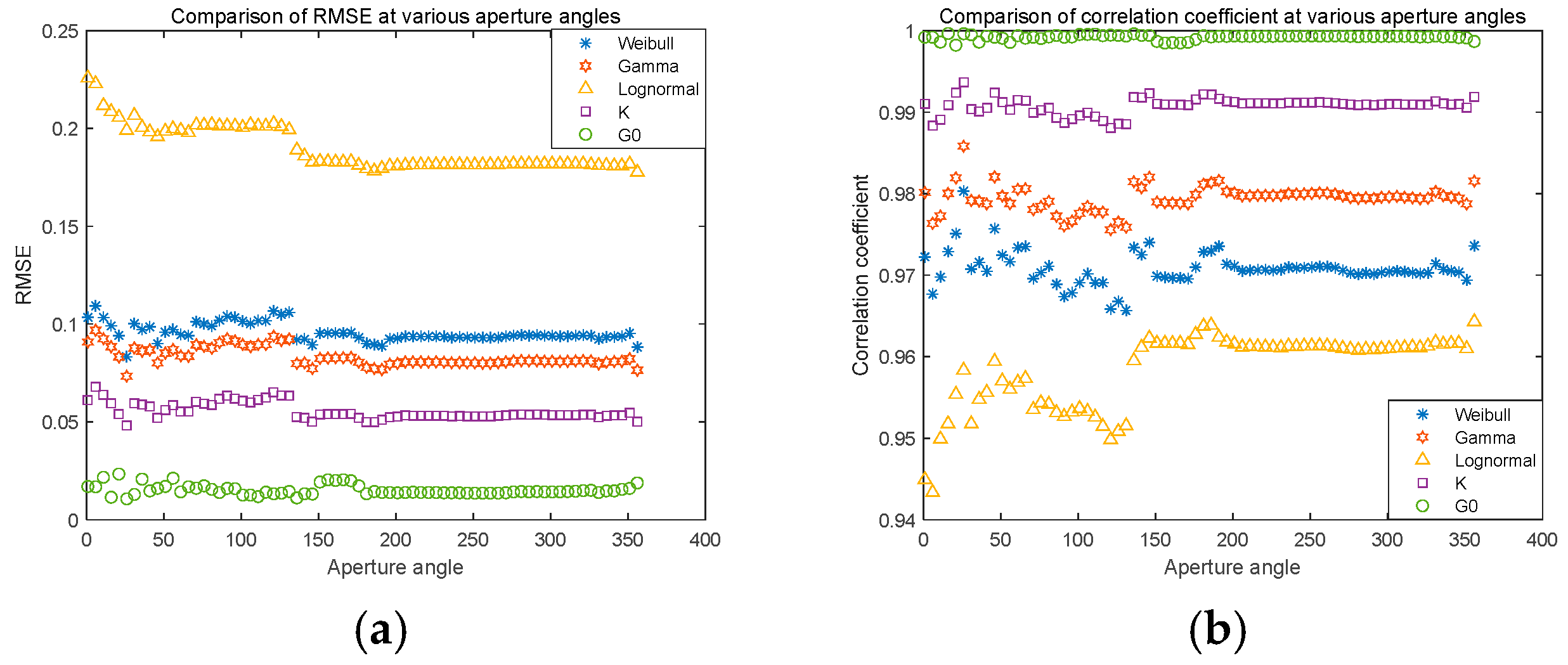
Aperture angle. Figure 7a–c show the modeling capability (evaluated by the three fitting optimization indexes introduced in Section 3.3) of the five single-parametric models for the isotropic region in the C-band Zhuhai data outlined in the red boxes in Figure 4a. The amplitude scatter histogram and fitting results for the best-fitting and aperture angles of the isotropic region are shown in Figure 7d. Further details regarding the corresponding optimal model and fitting optimization indexes can be found in Appendix A 

Table A1. The best-fitting single-parametric models and corresponding fitting optimization index for the optimal observation aspects and aperture angles in the X-band and C-band isotropic regions.

Analyzed Band	Selected Dimension	Best-Fitting Model	Optimal Aspect	RMSE	Correlation Coefficient	${\mathit{R}}_{\mathit{a}\mathit{d}\mathit{j}}^2$
X-band	aperture	Weibull	$114°$	0.0056	0.9998	0.9995
	observation	G0	$79°$	0.0037	0.9999	0.9998
C-band	aperture	G0	$125°$	0.0072	0.9996	0.9992
	observation	Weibull	$331°$	0.0068	0.9997	0.9993

.

As can be seen in Figure 7a–c, when modeling the statistical distribution characteristics of the isotropic regions for various aperture angles in the C-band Zhuhai data, the G0 distribution outperformed the Weibull distribution, followed by the Gamma distribution. The K distribution was slightly worse than Gamma, while the Log-normal performed poorly. To further illustrate the modeling capabilities of the different models, we selected the one with the best fitting results among the 360 fitting results for the five single-parametric models for 72 aperture angles. The fitting results of the five models in the scatter histograms at the corresponding aperture angles are shown in Figure 7d. It can be seen that the G0 distribution fit the amplitude scatter histogram of the isotropic region at this aperture angle better compared with the other models, particularly the portion after the peak value, before the slope changes sharply. However, it performed poorly on the portions before and near the peak value and where the slope changes steeply after the peak value.

As for the X-band, the fitting results for the different aperture angles were similar to those of the C-band, except the modeling ability of the Weibull distribution was better than that of the G0 distribution in most cases. Detailed results can be found in Appendix A Figure A1 and Table A1.

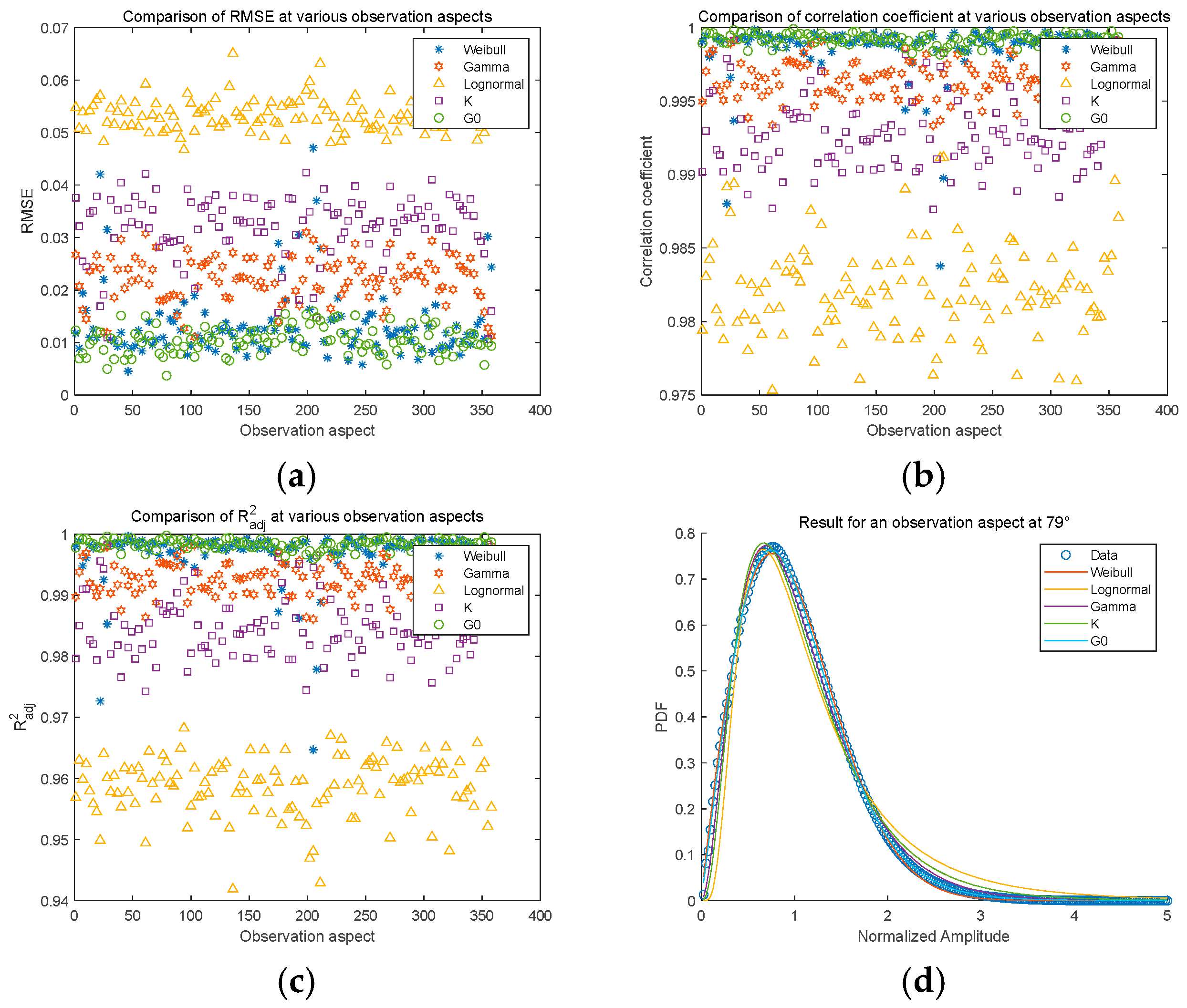
Observation aspects. Similarly, we analyzed the statistical distribution characteristics of the same isotropic region in the C-band for the different observation aspects. The results are shown in Figure 8.

By comparing Figure 8, it can be seen that the modeling capabilities of the various single-parametric models for the isotropic region at different observation aspects were similar to those for the various aperture angles. For example, in most cases, the G0 distribution demonstrated the strongest modeling capability for the isotropic region for the various observation aspects and aperture angles, whereas the Log-normal distribution performed the weakest. However, the modeling capability of the same single-parametric model varied depending on the changes in the observation aspects and aperture angles. Specifically, the fitting optimization indexes of the single-parametric models changed smoothly with the aperture angles but fluctuated with the observation aspects.

As for the X-band, the fitting results on the isotropic region for the various observation aspects were similar to those in the C-band. The fitting results varied depending on the change in the observation aspects and aperture angles, similar to those in the C-band. Detailed results can be found in Appendix A Figure A2 and Table A1. Apart from these similarities, there were still some subtle differences. To illustrate these differences, we calculated the proportion of angles (observation aspects or aperture angles) where each model achieved the best fitting results among all models under the three fitting indexes in two bands. In other words, the proportion was calculated as the number of angles (i.e., observation aspects or aperture angles) where each model has the strongest modeling ability divided by the total number of angles (i.e., observation aspects or aperture angles). The results are shown in

Table 2. Modeling capabilities of the single-parametric models on the isotropic regions.

Analyzed Region	Selected Dimension	Special Model	RMSE	Correlation Coefficient	${\mathit{R}}_{\mathit{a}\mathit{d}\mathit{j}}^2$
X-band	aperture	G0	36.7%	37.5%	36.7%
		Weibull	63.3%	62.5%	63.3%
		others	0.0%	0.0%	0.0%
	observation	G0	66.7%	66.7%	66.7%
		Gamma	0.0%	0.8%	0.0%
		K	0.8%	0.0%	0.8%
		Weibull	32.5%	32.5%	32.5%
		others	0.0%	0.0%	0.0%
C-band	aperture	G0	77.8%	80.6%	77.8%
		Weibull	22.2%	19.4%	22.2%
		others	0.0%	0.0%	0.0%
	observation	G0	83.3%	83.3%	83.3%
		Weibull	16.7%	16.7%	16.7%
		others	0.0%	0.0%	0.0%

.

As can be seen in the table, the G0 distribution and Weibull distribution were capable of modeling the statistical distribution characteristics of the isotropic region at various observation aspects and aperture angles in different bands quite well. In most cases, the G0 distribution outperformed the Weibull distribution. However, the Weibull distribution had an advantage in modeling the statistical distribution characteristics of the X-band under various aperture angles. For the X-band, the K distribution was the optimal model for one observation aspect according to the RMSE and $R_{adj}^2$ indexes, and the Gamma distribution was the optimal model at one observation aspect, according to the correlation coefficient index. Therefore, there are subtle differences in the modeling capabilities of the various models for the different fitting indexes. Although the G0 and Weibull distributions provide good modeling of the isotropic regions for most observation aspects and aperture angles, the K and Gamma distributions have their own advantages in certain specific cases.

In summary, the G0 and Weibull distributions performed well in modeling the statistical distribution characteristics of the isotropic regions under various observation aspects and aperture angles. However, both models still struggled to accurately represent the amplitude scatter histogram for the portions near the peak value and where the slope changed steeply after the peak value. In addition, the modeling capability of the same single-parametric models varied depending on the changes in observation aspects and aperture angles.

3.4.2. Anisotropic Regions

Similar to the isotropic regions, we analyzed the statistical distribution characteristics of the anisotropic regions for the various aperture angles and observation aspects in the C-band and X-band.

Aperture angle. Based on the C-band Zhuhai data outlined in the yellow boxes in Figure 4a, we analyzed the modeling capabilities of the five single-parametric models for the anisotropic region. The results are shown in Figure 9.

Figure 9a–c show that the G0 distribution achieved the best fitting performance for the anisotropic region at all aperture angles. Unlike the isotropic region in the C-band, the K distribution and Gamma distribution outperformed the Weibull distribution in modeling the anisotropic region, while the modeling capability of the Log-normal distribution became even weaker. Similar to the isotropic region in the C-band, we selected the best one from the 360 fitting results. Figure 9d shows the fitting results of the five models for the scatter histogram at the corresponding aperture angle. It can be seen that the G0 distribution achieved the best performance in fitting the amplitude scatter histogram of the anisotropic region at this aperture angle. It could fit most regions of the amplitude scatter histogram well but performed poorly on the portions near the peak value and where the slope changed steeply after the peak value.

As for the X-band, the fitting results for the anisotropic region at the various aperture angles were similar to those in the C-band. Therefore, we will not elaborate further here. Detailed results can be found in Appendix A, Figure A3, and

Table A2. The best-fitting single-parametric models and corresponding fitting optimization index for the optimal observation aspects and aperture angles in the X-band and C-band anisotropic regions.

Analyzed Band	Selected Dimension	Best-Fitting Model	Optimal Aspect	RMSE	Correlation Coefficient	${\mathit{R}}_{\mathit{a}\mathit{d}\mathit{j}}^2$
X-band	aperture	G0	$36°$	0.0141	0.9994	0.9985
	observation	G0	$31°$	0.0089	0.9997	0.9993
C-band	aperture	G0	$30°$	0.0107	0.9996	0.9992
	observation	G0	$26°$	0.0071	0.9998	0.9996

.

Observation aspects. Similarly, we analyzed the same anisotropic region in the C-band from the perspective of the observation aspects. The results are shown in Figure 10.

By comparing Figure 9 and Figure 10, we can draw the same conclusion for the isotropic region, i.e., the modeling capabilities of the various single-parametric models for the statistical distribution characteristics of the isotropic region at the various observation aspects are similar. However, unlike the isotropic region, for the anisotropic region, the fitting indexes of the single-parametric models varied more dramatically with the observation aspects. This is because the backscattering of the anisotropic regions is unstable and changes with the observation aspect. Thus, the modeling capabilities of the single-parametric models for the anisotropic regions fluctuated greatly with the observation aspect. Furthermore, it can be seen that the models with stronger modeling capabilities (such as the G0) exhibited less fluctuation with changes in the observation aspect, while models with weaker modeling capabilities (such as Log-normal) showed more drastic fluctuation with changes in the observation aspects.

As for the X-band, the fluctuation in the fitting results with the observation aspects and aperture angles was similar to that in the C-band. However, contrary to the C-band, the modeling capability of the Weibull distribution was better than those of the K distribution and Gamma distribution in most cases. The fitting results of each model for the anisotropic region at the different observation aspects in the X-band are shown in Appendix A, Figure A4, and Table A2.

Table 3. Modeling capabilities of the single-parametric models for the anisotropic regions.

Analyzed Region	Selected Dimension	Special Model	RMSE	Correlation Coefficient	${\mathit{R}}_{\mathit{a}\mathit{d}\mathit{j}}^2$
X-band	aperture	G0	100.0%	99.2%	100.0%
		K	0.0%	0.8%	0.0%
		others	0.0%	0.0%	0.0%
	observation	G0	78.3%	75.8%	77.5%
		Weibull	15.8%	17.5%	16.7%
		Gamma	4.2%	5.0%	4.1%
		K	1.7%	1.7%	1.7%
		others	0.0%	0.0%	0.0%
C-band	aperture	G0	100.0%	100.0%	100.0%
		others	0.0%	0.0%	0.0%
	observation	G0	100.0%	100.0%	100.0%
		others	0.0%	0.0%	0.0%

further demonstrates the differences in the fitting results of each model for the anisotropic regions at various aperture angles and observation aspects in the two bands.

As can be seen from the table, in the vast majority of cases, the G0 distribution demonstrated the best modeling capability for the statistical distribution characteristics of the anisotropic regions at the various observation aspects, as well as aperture angles in the different bands. However, the Weibull distribution, Gamma distribution, and K distribution each have certain advantages in modeling the anisotropic region for the various observation aspects in the X-band.

Thus, when modeling the statistical distribution characteristics of anisotropic regions at various observation aspects and aperture angles, the G0 distribution exhibited the best performance in most cases. However, it still suffers from low accuracy at the portions near the peak value and where the slope changes steeply after the peak value. In addition, the fitting indexes of the single-parametric models varied dramatically with the observation aspect.

3.5. Summary

Based on the qualitative and quantitative analysis of the statistical distribution characteristics of isotropic and anisotropic regions in multi-aspect SAR image, we find the following features that the statistical distribution characteristics of multi-aspect SAR possess (Q1).

First, the statistical distribution characteristics of isotropic targets in multi-aspect SAR images remain stable with changes in observation aspects and aperture angles. While for anisotropic targets, the statistical distribution characteristics of them in multi-aspect SAR images may change with observation aspects and aperture angles.

Second, for a multi-aspect SAR image, if the statistical distribution characteristics of its anisotropic regions can be well modeled by a model, then the same model can also effectively model those of its isotropic regions. In general, the models that can accurately model the statistical distribution characteristics of multiple terrain types in high resolution SAR images tend to be more flexible and adaptable. They can also model the statistical distribution characteristics of single terrain type in low resolution SAR images.

Finally, different regions of multi-aspect SAR images may exhibit distinct statistical distribution characteristics for the various observation aspects and aperture angles, which cannot be accurately modeled by an independent single-parametric model. In fact, each of these five single-parametric models has its own strengths and features. In the most cases, the G0 distribution has the strongest modeling capability among the five models. It can accurately model the statistical distribution characteristics of isotropic regions and anisotropic regions in multi-aspect SAR images for the various observation aspects and aperture angles. This is consistent with the characteristic that the G0 distribution can model the statistical distribution characteristics of various types of targets well as mentioned in Section 3.2. However, it still struggles to accurately model certain parts of the amplitude scatter histogram. In summary, although the G0 distribution is better than the other four distributions in modeling the statistical distribution characteristics of multi-aspect SAR images, it still struggles with many details of the amplitude scatter histogram. Its modeling capability is influenced by the target type, observation aspect, and aperture angle.

In view of the above analysis, none of the five single-parametric models can accurately model the statistical distribution characteristics of multi-aspect SAR images. This is because the increase in angle dimensions in multi-aspect SAR will bring about the improvement in resolution and the increase in scattering information. As a result, the terrain types in multi-aspect SAR are more mixed and the statistical distribution characteristics are more complex. Then, is there any model that can accurately model the statistical distribution characteristics of multi-aspect SAR images (Q2)?

4. Methodology

From the analysis in Section 3 regarding the statistical distribution characteristics of multi-aspect SAR images and the modeling capabilities of five single-parametric models, we find that different models have different advantages. Specifically, the G0 distribution generally provides the best modeling capabilities for the statistical distribution characteristics of different types of targets in multi-aspect SAR images for the various observation aspects and aperture angles. The K distribution performs well in modeling the statistical distribution characteristics of multi-aspect SAR images in most cases. In some specific cases, its modeling capability can surpass that of the G0 distribution. The Weibull and Gamma distributions have fewer parameters, simpler parameter estimation, and lower time complexity, while still maintaining reasonable modeling accuracy. Although the Log-normal distribution does not perform ideally for modeling anisotropic targets in multi-aspect SAR images, it has fewer parameters and can effectively model the statistical distribution characteristics of isotropic regions, sea clutter, and certain building regions in multi-aspect SAR images. Additionally, the interpretability of the Log-normal distribution is stronger than that of the Weibull distribution.

However, although we know the advantages and disadvantages of each model, we still cannot know which model to use to model them better, because the complexity of different regions in multi-aspect SAR images is different. In addition, the statistical distribution characteristics of the same region may differ for the various aperture angles and observation aspects. Thus, it is difficult to know in advance which specific single-parametric model would provide the best fit. In extreme cases, the terrain type may be extremely complex, and the statistical distribution characteristics may change dramatically for the various aperture angles and observation aspects. In this case, combining only a few single-parametric models would not achieve an accurate modeling of this region. Based on this consideration, we combine the five single-parametric models linearly and propose an FMM to explore the feasibility of accurate accurately modeling the statistical distribution characteristics of multi-aspect SAR (Q2). The following sections will introduce the FMM we proposed and its processing workflow and related technical details in modeling the statistical distribution characteristics of multi-aspect SAR images.

4.1. Finite Mixture Model

Multi-aspect SAR can observe the target scenes from multiple aspects and it has larger observation aspects and aperture angles than conventional SAR. Through multi-aspect observations and coherent and non-coherent imaging processing, it obtains multi-aspect scattering images with high resolution and improved signal-to-noise ratio (SNR). The improvement in resolution and the increase in angle dimensions reveal more detailed information about the terrain features. As a result, its scattering characteristics and statistical distribution characteristics are more complicated. Therefore, existing single-parametric models proposed for modeling the statistical distribution characteristics of conventional SAR images are not suitable for that of multi-aspect SAR images. The semiparametric FMM is a flexible and probabilistic modeling tool for both univariate and multivariate data. It is successfully applied in many fields such as pattern recognition, signal and image analysis, machine learning, and remote sensing. In the field of SAR image statistical distribution characteristics analysis, the FMM models the unknown PDF of amplitude or intensity images as a linear combination of parametric mixture components. Each single-parametric model of mixture component corresponds to a specific type of terrain. The FMM can increase the number of variables in the model, thereby enhancing the degrees of freedom and flexibility of the mixture model. This improves the capability to model the statistical distribution characteristics of multi-aspect SAR images. The FMM proposed in this paper models the amplitude scatter histogram of multi-aspect SAR images as a linear combination of the five single-parametric models commonly used in conventional SAR (introduced in Section 3.2). The formula is as follows:

$$f_{FMM}\left(r|\theta \right)=\sum _{i=1}^5{c}_i{f}_i\left(r|{\theta }_i\right) r\ge 0$$

(9)

where $f_i\left(r|{\theta }_i\right),i=1,2,\dots ,5$ represents five single-parametric models commonly used for conventional SAR images, including the Gamma distribution, Log-normal distribution, Weibull distribution, K distribution, and G0 distribution. $\theta =\left({\theta }_1,c_1,\dots {\theta }_5,c_5\right)$ is the parameter set of the FMM, encompassing parameters of each single-parametric model and their corresponding coefficients. $c_i$ is the coefficient corresponding to the model $f_i\left(r|{\theta }_i\right)$, satisfying the condition $\sum _{i=1}^5{c}_i=1,0\le c_i\le 1$.

4.2. The Workflow of FMM

Figure 11 illustrates the workflow of FMM modeling the statistical distribution characteristics of multi-aspect SAR images. The specific process is as follows:

Step 1: First, use the BP imaging algorithm to image the echo data to obtain ground range sub-aperture images of local cartesian coordinate.

Step 2: Analyze the statistical distribution characteristics of the multi-aspect SAR images from both different observation aspects and aperture angles.

Step 3: Select regions of interest from images for the various observation aspects and different aperture angles respectively.

Step 4: Normalize the images of the selected region in step 3 to obtain their amplitude scatter histograms.

Step 5: Employ the simulated annealing (SA) algorithm to estimate the parameters and corresponding coefficients of the five single-parametric models, obtaining the FMM that can accurately model the statistical distribution characteristics of the selected regions in multi-aspect SAR images.

Step 6: Fit the amplitude scatter histograms of the selected regions using the FMM obtained in step 5, and derive three fitting optimization indexes.

The key step in the workflow of FMM modeling the statistical distribution characteristics of multi-aspect SAR images is the parameter estimation of parameters of each single-parametric model and their corresponding coefficients. This estimation is implemented using the SA algorithm. The following two subsections will detail the parameter estimation process of FMM using the SA algorithm, and the perturbation algorithm improving the SA algorithm to ensure that the sum of the coefficients corresponding to the single-parametric models equals 1.

Figure 11. The workflow of FMM.

Figure 11. The workflow of FMM.

4.2.1. Simulated Annealing Algorithm

FMM encompasses a large number of parameters, including the parameters of each single-parametric model and their corresponding coefficients. However, traditional parameter estimation methods often struggle to implement effective parameter estimation.

Currently, the SA algorithm has been widely used in various fields, such as for the optimal design of ultra-large-scale integrated circuits, image processing, and neural network computations, proving to be effective in solving complex optimization problems. Given these advantages, we selected the SA algorithm to achieve the estimation of the FMM and accurately model the statistical distribution characteristics of multi-aspect SAR images.

The SA algorithm is a probabilistic optimization method inspired by the annealing process in metallurgy, where materials are heated and then cooled in a controlled manner to change their physical properties. The SA algorithm begins with a high initial temperature and iteratively decreases the temperature by multiplying it with a cooling rate until it reaches a predefined threshold. At each iteration, new parameters for the target model, such as the FMM, are generated. These new parameters are accepted based on a probability determined by the current temperature. Once the temperature reaches the threshold, the parameters and coefficients corresponding to the best-fitting optimization index across all iterations are chosen as the final model parameters.

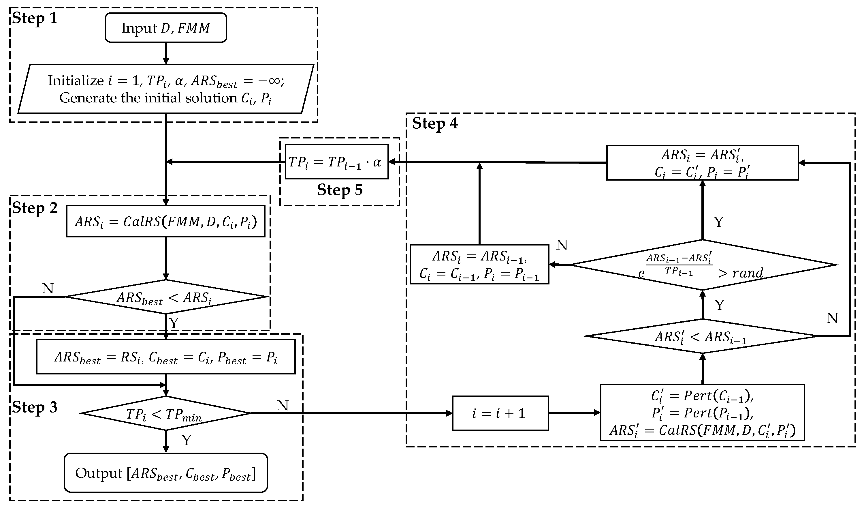
In this paper, we use the adjusted coefficient of determination, $R_{adj}^2$, to obtain the final FMM, because the $R_{adj}^2$ index accounts for the model’s complexity by applying a penalty to the number of parameters and can mitigate the overfitting issue. Figure 12 illustrates the workflow of the SA algorithm, and

Table 4. Notation table for the SA algorithm.

Notation	Description
$D$	The data consisted of the amplitude scatter histogram of the selected region in the multi-aspect SAR image.
$FMM$	The FMM which has coefficients and parameters that need to be estimated.
${TP}_i$	The temperature in the ith iteration. TP1 is the initial temperature. TPmin is the given minimum temperature, acting as the threshold to stop the iteration of the SA algorithm.
$\alpha$	The cooling rate to decrease the temperature of the SA algorithm.
${ARS}_i$	The adjusted coefficient of determination (namely, $R_{adj}^2$) in the ith iteration ${ARS}_{best}$ indicates the best fitting results obtained by the SA algorithm, which is set to−∞ initially.
$C_i$	The set of coefficients corresponding to each single-parametric model in the ith iteration. $C_{best}$ corresponds to ${ARS}_{best}$, which means the FMM fits the given data best.
$P_i$	The set of the parameters of the five single-parametric model in the ith iteration. $P_{best}$ corresponds to ${ARS}_{best}$, which means the FMM fits the given data best.
$rand$	A random number that is used to determine whether to accept the newly generated parameters and coefficients that result in a worse fit for FMM to the given data. This is important to avoid getting trapped in local optima.
$CalRS\left(\right)$	Calculate the $R_{adj}^2$ given the FMM, data, coefficients, and parameters.
$Pert\left(\right)$	The perturbation algorithm that generated new coefficients and parameters from old ones for each iteration. This algorithm is introduced in Section 4.2.2.

provides the notation table used in the workflow. As shown in Figure 12, the SA algorithm has the following steps:

Step 1: Given the data, $D$, and the finite mixture model, $FMM$, initialize the iteration counter, $i=1$; the initial temperature, ${TP}_i$; the cooling rate, $\alpha$; and set the optimal adjusted coefficient of determination, ${ARS}_{best}=-\infty$. Next, generate the initial parameters, $P_i$, for the five single-parametric models and the initial coefficients, $C_i$, for each single-parametric model. Finally, calculate the $R_{adj}^2$ value for the initial parameters and coefficients, denoted as ${ARS}_i$.

Step 2: Check whether the current ${ARS}_i$ surpasses the current optimal value ${ARS}_{best}$. If so, update the optimal parameter, $P_{best}$, the optimal coefficients, $C_{best}$, and the optimal adjusted coefficient of determination, ${ARS}_{best}$, with $P_1$, $C_1$, and ${ARS}_1$, respectively.

Step 3: Check whether the current temperature is below the given minimum temperature, ${TP}_{min}$. If so, output the current optimal result as the final FMM.

Step 4: Perturb the current parameters, $P_i$, and coefficients, $C_i$, to generate new ones (the perturbation algorithm is introduced in Section 4.2.2). If the $R_{adj}^2$ of the new parameters and coefficients are higher than the current ones, update the current parameters and coefficients to the new ones. If not, probabilistically update the current parameters and coefficients according to the expression $exp\left({\displaystyle \frac{{ARS}_{i-1}-A{RS}_i^{‘}}{{TP}_{i-1}}}\right)$ in order to avoid getting trapped in the local optima.

Step 5: Update the temperature and proceed to Step 2 to perform the next update iteration until the final FMM satisfying the requirements is obtained.

4.2.2. Perturbation Algorithm

For each iteration, the parameters can be conveniently perturbed by adding or subtracting a very small random number. However, the perturbing of the coefficients is relative complex. Specifically, the FMM is essentially a probability density function that must satisfy the property of integrating to 1. Therefore, the perturbation algorithm of the SA algorithm that is used to estimate the coefficients corresponding to each single-parametric model differs from traditional ones. To satisfy this property, we propose a novel perturbation algorithm.

Figure 13 illustrates a schematic diagram of the proposed perturbation algorithm used for parameter estimation of the coefficients corresponding to each single-parametric model. Generally, to obtain the coefficients corresponding to $m$ single-parametric models in the mixture model, we first select the $m+1$ coefficient splitting points, denoted as ${CS}_0, {CS}_1,{CS}_2\dots ,{CS}_{m-1}, {CS}_m$, where ${CS}_0$ is assigned a value of 0, and ${CS}_m$ is assigned a value of 1. To generate a new solution, we perturb ${CS}_i\left(i=1,2,\dots ,m-1\right)$ by adding or subtracting a very small random number, ensuring the relative order of the CS_i values is maintained. Finally, the coefficients $c_i \left(i=1,2,\dots ,m\right)$ corresponding to each single-parametric model are obtained by calculating ${CS}_i$. This perturbation algorithm guarantees that the sum of the coefficients $c_i \left(i=1,2,\dots ,m\right)$ equals 1. Consequently, this ensures that the integration of the finite mixture model, $FMM$, is equal to 1. The proof is as follows:

$$\begin{gathered} {\int }_0^{+\infty }FMM\left(x\right)dx={\int }_0^{+\infty }\left({\sum }_{i=1}^m{c}_i·{SM}_i\right)dx \\ ={\sum }_{i=1}^m{\int }_0^{+\infty }\left(c_i·{SM}_i\right)dx \\ ={\sum }_{i=1}^m\left(c_i{\int }_0^{+\infty }{SM}_{i}dx\right) \\ ={\sum }_{i=1}^m{c}_i \\ =1 \end{gathered}$$

(10)

5. Experiment and Results

We continued to use the C-band Zhuhai and X-band GOTCHA data introduced in Section 2.2 to evaluate the proposed FMM in Section 4. According to the analysis in Section 3, the models that can accurately model the statistical distribution characteristics of anisotropic regions can also model isotropic regions precisely. Thus, without loss of generality, we select anisotropic man-made targets as research objects in this section. In Section 3, to more intuitively demonstrate the statistical distribution characteristics of anisotropic regions, we selected a simple and relatively ideal target for analysis. However, in practical applications, the target regions are generally larger, with more complex scenes and structures. Based on this consideration, to provide theoretical support for future applications in the real world, we selected more complex regions that are closer to real-world scenarios to explore the feasibility of the FMM in accurately modeling the statistical distribution characteristics of multi-aspect SAR images. In the C-band Zhuhai data, the building outlined in the green box in Figure 14b is the largest independent anisotropic man-made target region in the scene. In the X-band GOTCHA data, the vehicle outlined in the green box in Figure 14a is the largest anisotropic man-made target region in the scene. In addition, buildings and vehicles are common anisotropic targets in real scenes. Thus, we chose these two regions to research.

By comparing the fitting optimization indexes (introduced in Section 3.3) obtained from modeling the statistical distribution characteristics of these two anisotropic regions for the various observation aspects and aperture angles using the five single-parametric models (introduced in Section 3.2) and the FMM (proposed in Section 4), we explore the feasibility of the FMM to model the statistical distribution characteristics of multi-aspect SAR images.

5.1. Aperture Angle

In this section, we use the FMM and five single-parametric models to analyze the statistical distribution characteristics of the C-band building region and the X-band vehicle region. Furthermore, we explore the feasibility of FMM in accurately modeling the statistical distribution characteristics of multi-aspect SAR images for the various aperture angles.

C-band building region. we present the fitting results obtained from modeling the statistical distribution characteristics of this region using the six modeled in Figure 15a,c,e. In Figure 15b,f, the $R_{adj}^2$ and correlation coefficients of the six models are magnified along the vertical axis to further show the modeling capabilities of the FMM for the statistical distribution characteristics of the selected region. The amplitude scatter histogram and fitting results for the best-fitting and aperture angles of the building region are shown in Figure 15d.

From Figure 15, we can see that compared with the five single-parametric models, FMM has the smallest RMSE (Figure 15c), the highest correlation coefficient (Figure 15e) and $R_{adj}^2$ (Figure 15a) under most aperture angles, which indicates that the FMM performed the best in most cases. In addition, the RMSE, $R_{adj}^2$ and correlation coefficient of the FMM had the least variation and fluctuation with the aperture angles. Therefore, the FMM can accurately model the statistical distribution characteristics of anisotropic regions in multi-aspect SAR images for the various aperture angles. In addition, we selected four aperture angles (i.e., 90°, 180°, 270°, and 360°) and provided the detailed fitting results in Appendix A,

Table A3. Fitting results of the X-band GOTCHA data for the various aperture angles.

Angle	Model	RMSE	Correlation Coefficient	${\mathit{R}}_{\mathit{a}\mathit{d}\mathit{j}}^2$
$90°$	Weibull	0.0356	0.9941	0.9829
	Gamma	0.0255	0.9966	0.9912
	Log-normal	0.0819	0.9736	0.9097
	K	0.0265	0.9957	0.9905
	G0	0.0154	0.9986	0.9968
	FMM	0.0048	0.9998	0.9997
$180°$	Weibull	0.0419	0.9913	0.9753
	Gamma	0.0277	0.9962	0.9892
	Log-normal	0.0783	0.9780	0.9140
	K	0.0241	0.9966	0.9918
	G0	0.0140	0.9987	0.9972
	FMM	0.0074	0.9996	0.9992
$270°$	Weibull	0.0379	0.9921	0.9792
	Gamma	0.0216	0.9976	0.9932
	Log-normal	0.0703	0.9835	0.9285
	K	0.0176	0.9980	0.9955
	G0	0.0087	0.9995	0.9989
	FMM	0.0061	0.9997	0.9994
$360°$	Weibull	0.0430	0.9907	0.9750
	Gamma	0.0263	0.9967	0.9906
	Log-normal	0.0851	0.9792	0.9017
	K	0.0206	0.9976	0.9942
	G0	0.0083	0.9996	0.9991
	FMM	0.0043	0.9999	0.9997

and

Table A4. Fitting results of the C-band Zhuhai data for the various aperture angles.

Angle	Model	RMSE	Correlation Coefficient	${\mathit{R}}_{\mathit{a}\mathit{d}\mathit{j}}^2$
$90°$	Weibull	0.0395	0.9920	0.9822
	Gamma	0.0234	0.9973	0.9937
	Log-normal	0.1171	0.9878	0.8432
	K	0.0134	0.9990	0.9979
	G0	0.0238	0.9969	0.9935
	FMM	0.0035	0.9999	0.9999
$180°$	Weibull	0.0403	0.9922	0.9820
	Gamma	0.0224	0.9978	0.9944
	Log-normal	0.1221	0.9849	0.8346
	K	0.0113	0.9994	0.9986
	G0	0.0200	0.9979	0.9955
	FMM	0.0036	0.9999	0.9999
$270°$	Weibull	0.0383	0.9934	0.9839
	Gamma	0.0215	0.9982	0.9949
	Log-normal	0.1247	0.9836	0.8289
	K	0.0122	0.9994	0.9984
	G0	0.0171	0.9984	0.9967
	FMM	0.0041	0.9999	0.9998
$360°$	Weibull	0.0387	0.9930	0.9833
	Gamma	0.0222	0.9979	0.9945
	Log-normal	0.1220	0.9857	0.8341
	K	0.0123	0.9993	0.9983
	G0	0.0201	0.9978	0.9955
	FMM	0.0062	0.9998	0.9995

for reference. To further demonstrate the modeling capability of the FMM, among the 360 fitting results of the single-parametric models (72 aperture angles for each of the five single-parametric models), we selected the best one (i.e., the K distribution at 150°). Then, we compared the fitting results of the FMM and the five single-parametric models at the corresponding aperture angle (i.e., 150°). The comparison results are shown in Figure 15d. At this aperture angle, the fitting curve of the FMM was closer to the scatter histogram compared with the other models. Specifically, the FMM improved the fitting effect for the portion near the peak and where the slope changed steeply in the amplitude scatter histogram compared with the single-parametric models. The peak position of the FMM is closest to that of the amplitude scatter histogram. Therefore, the FMM achieves a better fit for the amplitude scatter histogram of the anisotropic building region at this aperture angle.

X-band vehicle region. We also analyzed the statistical distribution characteristics of the X-band vehicle region in the multi-aspect SAR images for the various aperture angles using the six models. The experimental results indicate that, compared with the other five single-parametric models, the FMM could also accurately model the statistical distribution characteristics of the anisotropic region for the various aperture angles in the X-band. Furthermore, the FMM provided better fitting results for the tail regions of the amplitude scatter histograms at some aperture angles compared with the five single-parametric models. Other experimental results are similar to those for the C-band and are not elaborated here. The detailed results can be referred to in Appendix A and Figure A5.

5.2. Observation Aspect

Similar to Section 5.1, we further analyzed the feasibility of FMM for accurately modeling the statistical distribution characteristics of multi-aspect SAR images with different observation aspects in different bands.

C-band building region. Figure 16 shows the fitting results of six models to the statistical distribution characteristics of the C-band building region in multi-aspect SAR images for the various observation aspects. The meaning of each subfigure in Figure 16 is consistent with that of Figure 15 in Section 5.1.

By comparing Figure 15 and Figure 16, we can see that the modeling capability of the FMM for the statistical distribution characteristics of multi-aspect SAR images for the various observation aspects is similar to those for the various aperture angles. First, in the vast majority of observation aspects, the FMM achieved the best RMSE, correlation coefficient, and $R_{adj}^2$ compared with the single-parametric models. Second, compared with the other models, the three fitting indexes of the FMM exhibited the smallest fluctuations with the change in the observation aspects. Thus, the FMM can accurately model the statistical distribution characteristics of anisotropic regions in multi-aspect SAR images for various observation aspects. Similar to Section 5.1, we selected four observation aspects, and the detailed fitting results are provided in Appendix A,

Table A5. Fitting results of the X-band GOTCHA data for the various observation aspects.

Aspect	Model	RMSE	Correlation Coefficient	${\mathit{R}}_{\mathit{a}\mathit{d}\mathit{j}}^2$
$90°$	Weibull	0.0379	0.9920	0.9796
	Gamma	0.0225	0.9973	0.9928
	Log-normal	0.0765	0.9824	0.9167
	K	0.0182	0.9980	0.9953
	G0	0.0102	0.9993	0.9985
	FMM	0.0093	0.9994	0.9987
$180°$	Weibull	0.0617	0.9887	0.9665
	Gamma	0.0456	0.9942	0.9817
	Log-normal	0.1711	0.9555	0.7423
	K	0.0375	0.9954	0.9875
	G0	0.0202	0.9984	0.9964
	FMM	0.0118	0.9994	0.9987
$270°$	Weibull	0.0372	0.9918	0.9802
	Gamma	0.0192	0.9980	0.9948
	Log-normal	0.0753	0.9869	0.9189
	K	0.0114	0.9992	0.9981
	G0	0.0087	0.9995	0.9989
	FMM	0.0064	0.9997	0.9994
$360°$	Weibull	0.0744	0.9839	0.9545
	Gamma	0.0561	0.9918	0.9741
	Log-normal	0.1830	0.9525	0.7243
	K	0.0403	0.9954	0.9865
	G0	0.0135	0.9993	0.9985
	FMM	0.0048	0.9999	0.9998

and

Table A6. Fitting results of the C-band Zhuhai data for the various observation aspects.

Aspect	Model	RMSE	Correlation Coefficient	${\mathit{R}}_{\mathit{a}\mathit{d}\mathit{j}}^2$
$90°$	Weibull	0.0489	0.9825	0.9632
	Gamma	0.0369	0.9901	0.9791
	Log-normal	0.0733	0.9964	0.9173
	K	0.0195	0.9971	0.9941
	G0	0.0302	0.9935	0.9859
	FMM	0.0064	0.9997	0.9993
$180°$	Weibull	0.0348	0.9910	0.9810
	Gamma	0.0202	0.9969	0.9936
	Log-normal	0.0659	0.9948	0.9320
	K	0.0119	0.9990	0.9978
	G0	0.0244	0.9955	0.9906
	FMM	0.0059	0.9997	0.9994
$270°$	Weibull	0.0374	0.9893	0.9779
	Gamma	0.0251	0.9951	0.9900
	Log-normal	0.0668	0.9952	0.9295
	K	0.0172	0.9978	0.9953
	G0	0.0303	0.9930	0.9855
	FMM	0.0035	0.9999	0.9998
$360°$	Weibull	0.0368	0.9897	0.9786
	Gamma	0.0227	0.9961	0.9919
	Log-normal	0.0651	0.9950	0.9331
	K	0.0136	0.9986	0.9971
	G0	0.0259	0.9949	0.9893
	FMM	0.0053	0.9998	0.9995

for reference. Following the method described in Section 5.1, we selected one observation aspect and presented the fitting results of the six models on the amplitude scatter histogram at this aspect in Figure 16d. From Figure 16d, it can be seen that at this observation aspect, the FMM outperformed the other five single-parametric models in fitting the steep slope changes in the amplitude scatter histogram. Therefore, the FMM had a superior fitting performance for the amplitude scatter histogram at this observation aspect compared with the other five single-parametric models.

X-band vehicle region. We also conducted experiments on the X-band, and the results are similar to those for the C-band. Detailed results can be found in Appendix A Figure A6. These experiment results indicate that among the six models, the FMM demonstrated the best modeling capability for the statistical distribution characteristics of multi-aspect SAR images for various observation aspects. Additionally, it can fit the tail regions of the amplitude scatter histograms well for some observation aspects in the X-band.

6. Discussion

To intuitively demonstrate the modeling capabilities of the six models for anisotropic regions at various observation aspects and aperture angles in different bands, we summarized the above fitting results.

Table 5. Modeling capabilities of the FMM and single-parametric models for anisotropic regions.

Analyzed Region	Selected Dimension	Model Type	Special Model	RMSE	Correlation Coefficient	${\mathit{R}}_{\mathit{a}\mathit{d}\mathit{j}}^2$
X-band	aperture	Single model	G0	100.0%	100.0%	100.0%
			others	0.0%	0.0%	0.0%
		Mixture model	FMM	100.0%	100.0%	100.0%
			others	0.0%	0.0%	0.0%
	observation	Single model	G0	100.0%	99.2%	100.0%
			Gamma	0.0%	0.8%	0.0%
			others	0.0%	0.0%	0.0%
		Mixture model	FMM	99.2%	99.2%	99.2%
			G0	0.8%	0.8%	0.8%
			others	0.0%	0.0%	0.0%
C-band	aperture	Single model	K	100.0%	100.0%	100.0%
			others	0.0%	0.0%	0.0%
		Mixture model	FMM	100.0%	100.0%	100.0%
			others	0.0%	0.0%	0.0%
	observation	Single model	K	90.3%	77.8%	90.3%
			G0	9.7%	9.7%	9.7%
			Log-normal	0.0%	12.5%	0.0%
			others	0.0%	0.0%	0.0%
		Mixture model	FMM	100.0%	100.0%	100.0%
			others	0.0%	0.0%	0.0%

presents the modeling capabilities of the five single-parametric models and the six models (five single-parametric models plus the FMM) for anisotropic regions of multi-aspect SAR images for various observation aspects and aperture angles in different bands. In the “Model type” column, the “Single model” indicates that only the five single-parametric models were compared, while “Mixture model” indicates that both the five single-parametric models and FMM were included in the comparison. The percentages for the various indexes represent the number of angles (observation aspects or aperture angles) in which each model achieved the best performance for the corresponding fitting index divided by the total number of angles (observation aspects or aperture angles).

By analyzing Table 5 in conjunction with Table 2 and Table 3, we drew the following conclusions:

• Each single-parametric model has its own applicable scenarios.
• Various fitting indexes have different feasibilities in evaluating the modeling capabilities of different models across various scenarios. To objectively assess the modeling capabilities of the models, the RMSE, correlation coefficient, and ${\mathit{R}}_{\mathit{a}\mathit{d}\mathit{j}}^2$ are all indispensable.
• Although the Log-normal distribution is not ideal for modeling the statistical distribution characteristics of multi-aspect SAR images in many cases, it still achieved the best correlation coefficient for 12.5% of observation aspects in the C-band.
• Compared with the five single-parametric models, the FMM can more accurately model the statistical distribution characteristics of multi-aspect SAR images under the vast majority of the observation aspects and aperture angles in different bands. However, for a few angles, the fitting effect of the FMM was slightly inferior. This is likely due to the increased difficulty in parameter estimation caused by the large number of parameters in the FMM. This issue can be improved in the future by reducing the number of components in the model or enhancing parameter estimation methods.

In summary, combining different models is an effective approach to develop a model capable of more accurately modeling the statistical distribution characteristics of multi-aspect SAR images (Q2). Future work can further explore strategies for model combinations to improve the performances in moving target detection, target extraction, and other related tasks for multi-aspect SAR images.

7. Conclusions

Multi-aspect SAR is an emerging observation mode that utilizes the radar platform to conduct azimuthal observations of scenes from various aspects. It can obtain information from these various aspects and provide a more comprehensive contour structure compared with conventional SAR. Accurate modeling of the statistical information in multi-aspect SAR images is crucial for its processing and applications. In this paper, we qualitatively and quantitatively analyze the statistical distribution characteristics of multi-aspect SAR images across the following three dimensions: different terrain types, observation aspects, and aperture angles. The results show that the statistical distribution characteristics of the various regions in the multi-aspect SAR images varied depending on the changes in the observation aspect and aperture angle. The single-parametric models commonly used for conventional SAR images failed to accurately model the statistical distribution characteristics of the multi-aspect SAR images. In order to explore the feasibility of obtaining a model that can accurately model the statistical distribution characteristics of multi-aspect SAR images, we proposed an FMM and evaluated it on X-band GOTCHA data and C-band Zhuhai data. The evaluation’s results show that it can accurately model the statistical distribution characteristics of different types of targets in multi-aspect SAR images for various observation aspects and aperture angles in various bands. Therefore, combining different models is a promising direction that warrants further exploration to accurately model the statistical distribution characteristics of multi-aspect SAR images.