Multi-Decision Vector Fusion Model for Enhanced Mapping of Aboveground Biomass in Subtropical Forests Integrating Sentinel-1, Sentinel-2, and Airborne LiDAR Data

Abstract

The accurate estimation of forest aboveground biomass (AGB) is essential for effective forest resource management and carbon stock assessment. However, the estimation accuracy of forest AGB is often constrained by scarce in situ measurements and the limitations of using a single data source or retrieval model. This study proposes a multi-source data integration framework using Sentinel-1 (S-1) and Sentinel-2 (S-2) data along with eight predictive models (i.e., multiple linear regression—MLR; Elastic-Net; support vector regression (with a linear kernel and polynomial kernel); k-nearest neighbor; back-propagation neural network—BPNN; random forest—RF; and gradient-boosting tree—GBT). With airborne light detection and ranging (LiDAR)-derived AGB as a reference, a three-stage optimization strategy was developed, including stepwise feature selection (SFS), hyperparameter optimization, and multi-decision vector fusion (MDVF) model construction. Initially, the optimal feature subsets for each model were identified using SFS, followed by hyperparameter optimization through a grid search strategy. Finally, eight models were evaluated, and MDVF was implemented to integrate outputs from the top-performing models. The results revealed that LiDAR-derived AGB demonstrated a strong performance (R² = 0.89, RMSE = 20.27 Mg/ha, RMSE_r = 15.90%), validating its effectiveness as a supplement to field measurements, particularly in subtropical forests where traditional inventories are challenging. SFS could adaptively select optimal variable subsets for different models, effectively alleviating multicollinearity. Satellite-based AGB estimation using the MDVF model yielded robust results (R² = 0.652, RMSE = 31.063 Mg/ha, RMSE_r = 20.4%) through the synergy of S-1 and S-2, with R² increasing by 4.18–7.41% and the RMSE decreasing by 3.55–5.89% compared to the four top-performing models (BPNN, GBT, RF, MLR) in the second optimization stage. This study aims to provide a cost-effective and precise strategy for large-scale and spatially continuous forest AGB mapping, demonstrating the potential of integrating active and passive satellite imagery with airborne LiDAR to enhance AGB mapping accuracy and support further ecological monitoring and forest carbon accounting.

1. Introduction

Forest ecosystems are fundamental to the global carbon cycle, covering approximately 30% of the Earth’s surface and storing nearly 80% of terrestrial carbon [1,2]. As major carbon sinks, they regulate the climate, support biodiversity, and provide essential ecosystem services [3]. Aboveground biomass (AGB) serves as a key measure of carbon storage capacity, defined as the dry weight of living organic material above the soil surface, encompassing stems, stumps, branches, bark, seeds, and foliage [4]. However, accurate AGB estimation remains challenging due to many factors, such as the heterogeneity of forest structure, limited field measurements, and insufficient knowledge of forest density distribution [5,6]. These uncertainties hinder the precise assessments of forest carbon sequestration, complicating efforts to monitor forest dynamics and mitigate climate change [7]. Therefore, timely and accurate AGB mapping is crucial for monitoring the terrestrial carbon cycle and addressing global climate change.

Traditional in situ measurements of AGB are often labor-intensive, destructive, and spatially discontinuous over limited areas [8]. In contrast, satellite remote sensing has become indispensable for dynamic forest resource management, due to its rapid, non-invasive, and scalable data acquisition. Multispectral satellite data—particularly from the dual Sentinel-2 (S-2) satellites launched by the European Space Agency (ESA)—have emerged as a key resource for AGB estimation. With its high spatial and temporal resolution and the inclusion of three red-edge bands (RE), S-2 offers substantial potential for detailed AGB monitoring [9]. However, passive optical remote sensing is limited to capturing canopy surface spectral and horizontal texture information and is prone to saturation in dense forests, as well as contamination by atmospheric clouds, smoke, and dust [10]. Conversely, synthetic aperture radar (SAR), an active remote sensing technology, provides full-time and full-weather observation capabilities and can penetrate the forest canopy to retrieve valuable vertical structural information [11]. Prior studies have demonstrated notable correlations between forest structural parameters and C-band backscattering coefficients [12,13,14]. These findings have paved the way for using Sentinel-1 (S-1) C-band dual-polarization SAR to estimate forest AGB. Nevertheless, SAR data can be disturbed by topographic relief [15] and exhibit saturation in high-AGB regions [11]. Thus, the integration of both active and passive remote sensing data holds considerable promise for AGB modeling by effectively mitigating the limitations inherent in individual data sources.

Light detection and ranging (LiDAR) can acquire complex and detailed three-dimensional canopy information, enabling the precise estimation of forest structural parameters. Previous studies suggested that LiDAR-derived metrics, such as the leaf area index and canopy height, can achieve accuracies comparable to ground-measured data [16,17]. However, the precision of AGB estimates derived from LiDAR metrics has not been widely validated against in situ data. Additionally, airborne LiDAR data are not suitable for multi-temporal, large-scale, and spatially continuous applications. Therefore, integrating airborne LiDAR with optical and SAR satellite imagery represents a promising approach for large-scale, low-cost AGB estimation. In this framework, airborne LiDAR supplies high-quality AGB samples for training and validation, while satellite imagery serves as predictor variables for wall-to-wall mapping.

Challenges persist in selecting the optimal AGB retrieval model and managing data redundancy from multi-source data. Parametric models, prized for their simplicity and interpretability, often struggle to capture complex nonlinear relationships in heterogeneous areas and face the “curse of dimensionality” with high-dimensional data [18,19]. In contrast, non-parametric machine learning (ML) methods, data-driven and adept at modeling intricate nonlinearities, show considerable promise in inversion research [20]. Nevertheless, current studies develop and compare models independently, without integrating their outputs, potentially limiting retrieval capabilities due to model-specific shortcomings. Additionally, selecting informative and independent metrics is critical for accurate AGB estimation from multi-source data. Traditional methods often rely on specific non-parametric models, such as random forest (RF) [21], or on linear correlation measures like Pearson’s correlation coefficient [22] for feature selection. However, features extracted through a specific model may not generalize to others, and linear correlations alone cannot capture the complex nonlinear relationships between forest AGB and remote sensing data. Therefore, the combination of advanced ML models with robust, model-adaptive feature selection is imperative to overcome data redundancy and capture complex nonlinear relationships, ultimately enhancing the accuracy and reliability of forest AGB estimation.

As China’s largest economic province, Guangdong—an “oasis on the Tropic of Cancer” due to its unique hydrothermal conditions—faces a critical need for accurate forest AGB estimation to support ecological preservation amid rapid development. However, few studies have focused on AGB inversion in this region, particularly those employing integrated active and passive remote sensing.

This study aims to combine LiDAR-derived AGB with the synergy of active and passive remote sensing technology to optimize modeling approaches and improve AGB estimation in northeastern Conghua, Guangdong. A comprehensive analysis was conducted using multi-source data (S-2 and S-1, and their combination) and models (two parametric and six non-parametric). Overall, we proposed the triple stepwise optimization workflow: (ⅰ) developing a stepwise feature selection (SFS) method to adaptively extract the optimal variables for each model.; (ⅱ) optimizing hyperparameter to enhance model performance; and (ⅲ) constructing multi-decision vector fusion (MDVF) model using top-performing optimized models, enhancing accuracy and robustness.

2. Materials

2.1. Study Area

This study was conducted in the northeastern Conghua forest, Guangdong, China (23°52′35.65″N, 113°54′46.17″E), covering approximately 100 km², as shown in Figure 1 and corresponding to the extent of airborne LiDAR coverage. Elevations range from 197 m in the northeast to 621 m in the southwest. This region features a subtropical monsoon climate with an average annual rainfall of 1951.9 mm and a mean temperature of about 21.2 °C. The main vegetation types are evergreen broadleaved and needle-leaved forests, as reported in [23] (Figure 1), with species such as Schima superba, Castanopsis fissa, Cinnamomum porrectum, and Pinus massoniana.

2.2. Field Data Collection

The forest inventory conducted from mid-August to early September 2017 established 60 plots (30 m × 30 m each) within the LiDAR coverage area. In each plot, the diameter at breast height (DBH) and tree height (H) were measured for all trees with a DBH greater than 3 cm using a laser hypsometer and tape. The geographic coordinates of each plot were determined at the plot center using a Garmin MAP 60CS GPS (accuracy: ±3 m). Species names, types, and dominant land cover classes were also recorded. Plots with over 75% deciduous or coniferous trees were classified as deciduous or coniferous, respectively; otherwise, they were assigned as mixed forests [24].

For this study, we applied Fang’s method [25] to evaluate AGB for each sampling unit. Initially, individual tree volumes were calculated using a two-variable volume table based on the DBH and tree height, and then the total volume (TV) for each plot was obtained by summing the volumes of all trees within the plot. A regression model (Equation (1)) was subsequently used to convert the total volume to total AGB (TAGB) in megagrams per hectare (Mg/ha), with constants a and b set according to Fang et al. [25] to account for specific forest types.

$$\mathrm{TAGB}=a\times \mathrm{TV}+b$$

(1)

The biomass ranged from 16.98 to 277.27 Mg/ha, with a standard deviation of 70.77 Mg/ha, and an average value of 109.32 Mg/ha.

2.3. Remote Sensing Data Acquisition and Preprocessing

2.3.1. LiDAR Data Acquisition and Preprocessing

Discrete-return LiDAR data were collected in June 2017 using an Optech Gemini system aboard a Partenavia P68 fixed-wing aircraft. The dual-return system recorded up to two echoes per laser shot across twelve transects, each approximately 300 m wide, at a flight altitude of 850 m. With a 15° scan angle and a pulse frequency of 70 kHz, the survey achieved an average pulse density of 1.5 pulses per square meter. Finally, the airborne LiDAR data covered the entire study area of approximately 100 km². The point cloud data were preprocessed using TerraScan (v4.006, TerraSolid, Helsinki, Finland), including outlier removal, ground/non-ground classification, and height normalization. Outliers deviating significantly from median elevations were removed. Ground and non-ground points were separated to generate a 1 m resolution digital surface model (DSM) and digital elevation model (DEM). The canopy height model (CHM) was derived by subtracting the DEM from the DSM, retaining CHM values between 2 and 35 m to exclude undergrowth and anomalous objects.

2.3.2. Satellite Image Acquisition and Preprocessing

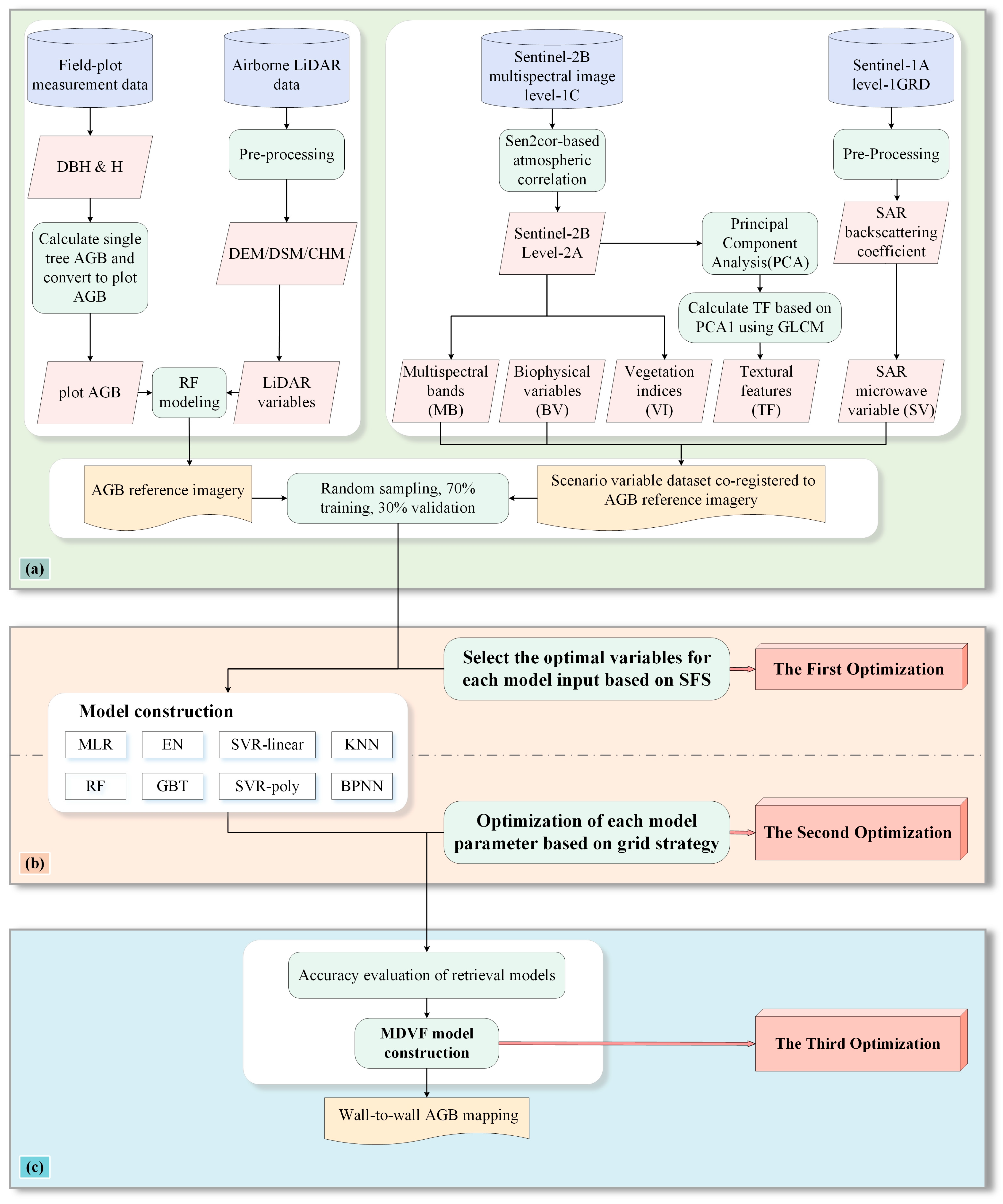
Sentinel-2B/Multispectral Instrument (MSI) Level-1C imageries, which provide atmospheric apparent reflectance and were acquired on 2 October 2018, were downloaded from the Copernicus Data Space Ecosystem (https://dataspace.copernicus.eu/, accessed on 27 July 2024). Atmospheric corrections were applied using the Sen2Cor tool in ESA’s SNAP v9.0.0 [26] to generate Level-2A data. Ten spectral bands, including visible, RE, near-infrared (NIR), and shortwave infrared (SWIR), were selected for further processing. We utilized Band 2 to Band 12, excluding the 60 m water vapor-related bands, as they are not relevant to this study. The 20 m resolution bands (i.e., Band 5, Band 6, Band 7, Band 8A, Band 11, and Band 12) were resampled to 10 m resolution using cubic convolution using the Geospatial Data Abstraction Library (GDAL) [27] in Python 3.

Sentinel-1 Ground Range Detected (GRD) data acquired on 27 September 2018 were obtained via Google Earth Engine (GEE) (https://code.earthengine.google.com/, accessed on 7 August 2024). The data, acquired in Interferometric Wide Swath mode with dual-polarization (VH and VV) at C-band (5.3 GHz), had a 10 m resolution and an average incidence angle of 37.6°. For this research, we employed the JavaScript-based API interface to import the GRD data, that is, ’COPERNICUS/S1_GRD’, in the ’Code Edit’ module of the GEE platform. Traditionally, SNAP was used to preprocess SAR data, encompassing several steps such as applying orbit files, processing thermal noise, speckle filters, radiometric calibration, topographic correction, and geocoding. In contrast, the result of the aforementioned preprocessing steps, the backscattering coefficient, could be employed immediately on the GEE platform.

Finally, we used GDAL programming to reproject the S-1 and S-2 data into the UTM/WGS84 coordinate system.

3. Methods

The AGB estimation workflow in this study, shown in Figure 2, includes (a) the extraction of multi-source remote sensing features and generation of an AGB reference map; (b) the feature selection, development, and optimization of AGB estimation models; and (c) the construction of the MDVF model and wall-to-wall AGB mapping using the optimized MDVF. Notably, SFS was applied to identify optimal input variables for each predictive model before modeling. It is important to note that in this study, airborne LiDAR data provided full coverage across the entire study area (~100 km²). However, in large-scale forest monitoring applications, LiDAR data are often acquired along discrete flight lines rather than as continuous coverage. Therefore, this study aimed to develop a scalable framework that links field plots with airborne LiDAR data and further extends LiDAR-derived AGB to satellite observations (S-1 and S-2), enabling continuous, large-area forest biomass mapping.

3.1. Extraction of Remote Sensing Variables

3.1.1. LiDAR Metrics

Twenty LiDAR indicators (see

Table 1. Metrics calculated from LiDAR data.

LiDAR Metrics	Abbreviation	Definition
Canopy height metric	Hmean,	Mean height above 2 m.
	Hmax	Maximum height.
	Hsd	Standard deviation of height above 2 m.
	Hvar	Variance of height above 2 m.
	Hcv	Coefficient of height variation above 2 m.
	Hp	Percentiles (50th, 55th, 60th, …, 85th, 90th, 95th) with a 5-unit height interval distribution above 2 m.
Canopy cover metric	LADa_b	The density of leaf area within the height range of a_b (2_10, 10_20, or 20_30).
	PDa_b	Ratio of first returns within a height range of a_b (2_10, 10_20, or 20_30) to the total number of first returns.
	CT	Canopy thickness above 2 m, H90th–H10th.
	CRR	Canopy relief ratio above 2 m.
	CCmean	Canopy cover above the mean height above 2 m.

) were derived from the first returns above 2 m to characterize the canopy structure. These indicators are divided into canopy cover and height indices: fifteen metrics capture the distribution and variability of canopy heights, while canopy cover variables reflect morphology and ecosystem functionality [28]. The canopy relief ratio (CRR) (see Equation (2)) quantifies the proportion of returns above the average height, and LAD_{a_b} and PD_{a_b} represent leaf area and point densities across height intervals, separately. All twenty indicators were derived from the LiDAR-derived 1 m CHM, aggregated to 10 m resolution through statistical computations (e.g., mean, maximum, percentile-based metrics).

$$\mathrm{CRR}={\displaystyle \frac{{\mathrm{H}}_{\mathrm{mean}}-{\mathrm{H}}_{\min }}{{\mathrm{H}}_{\max }-{\mathrm{H}}_{\min }}}$$

(2)

3.1.2. Active and Passive Remote Sensing Metrics

From the S-2 reflectance data, we extracted four groups of optical indicators across the study area: spectral bands, biophysical variables, vegetation indices, and texture features (see

Table 2. List of S-1 and S-2 predictors used for modeling.

Satellite	Data Scenarios	Predictor	Formula/Definition
Sentinel-1A (27 September 2018)	SAR Variables	VV	Vertical emission–vertical receipt
		VH	Vertical emission–horizontal receipt
		VV + VH	Sum
		VV − VH	Difference
		VV/VH	Cross-ratio
Sentinel-2B (2 October 2018)	Multispectral Bands	Band2	Blue; central wave length (CWL): 490 nm; spatial resolution (SP):10 m
		Band3	Green; CWL: 560 nm; SP:10 m
		Band4	Red (R); CWL: 660 nm; SP:10 m
		Band5	Red Edge1 (Edge1); CWL: 705 nm; SP:20 m
		Band6	Red Edge2 (Edge2); CWL: 705 nm; SP:20 m
		Band7	Red Edge3 (Edge3); CWL: 705 nm; SP:20 m
		Band8	Near infrared; CWL: 842 nm; SP:10 m
		Band8A	Narrow NIR; CWL: 842 nm; SP:20 m
		Band11	SWIR1; CWL: 1610 nm; SP:20 m
		Band12	SWIR2; CWL: 2190 nm; SP:20 m
	Vegetation Indices	SR	$NIR/R$
		NDVI	$(NIR-R)/(NIR+R)$
		TNDVI	$\sqrt{(NIR-R)/[(NIR-R)+0.5]}$
		EVI	$\left[2.5\times (NIR-R)\right]/(1+NIR+6\times R-7.5\times B)$
		IRECI	$(Edge3-R)/(Edge1/Edge2)$
		NDVIre1	$(NIR-Edge1)/(NIR+Edge1)$
		NDVIre2	$(NIR-Edge2)/(NIR+Edge2)$
		NDVIre3	$(NIR-Edge3)/(NIR+Edge3)$
		MDI1	$(NIR-SWIR1)/SWIR1$
		MDI2	$(NIR-SWIR2)/SWIR2$
	Biophysical Variables	LAI	Leaf area index
		FAPAR	Fraction of absorbed photosynthetically active radiation
		FVC	Fraction of vegetation cover
	Textural Features	Contrast (CON)	${\sum }_{i,j=0}^{N-1}i{P}_{i,j}{(i-j)}^2$
		Dissimilarity (DI)	${\sum }_{i,j=0}^{N-1}i{P}_{i,j}\left|i-j\right|$
		Homogeneity (HO)	${\sum }_{i,j=0}^{N-1}i{P}_{ij}/\left[1+{(i-j)}^2\right]$
		Second moment (SM)	${\sum }_{i,j=0}^{N-1}i{P}_{i,j}^2$
		Entropy (EN)	${\sum }_{i,j=0}^{N-1}i{P}_{i,j}(-\ln P_{i,j})$
		Mean (ME)	${\sum }_{i,j=0}^{N-1}i{P}_{i,j}$
		Variance (VA)	${\sum }_{i,j=0}^{N-1}i{P}_{i,j}(1-{\mu }_i)$
		Correlation (COR)	${\sum }_{i,j=0}^{N-1}i{\sum }_{i,j=0}^{N-1}i{P}_{i,j}-{\mu }_i{\mu }_j/{\sigma }_i^2{\sigma }_j^2$
	${\mu }_i={\displaystyle \sum _{i=0}^{N-1}i}{\displaystyle \sum _{j=0}^{N-1}{P}_{i,j};} {\mu }_i={\displaystyle \sum _{j=0}^{N-1}j}{\displaystyle \sum _{j=0}^{N-1}{P}_{i,j};} {\sigma }_i^2={\displaystyle \sum _{i=0}^{N-1}{(i-{\mu }_i)}^2}{\displaystyle \sum _{j=0}^{N-1}{P}_{i,j};} {\sigma }_j^2={\displaystyle \sum _{j=0}^{N-1}{(j-{\mu }_j)}^2}{\displaystyle \sum _{j=0}^{N-1}{P}_{i,j}}$

). To take full advantage of the broad spectral range of S-2 and its sensitivity to AGB, we calculated ten vegetation indices, particularly those involving SWIR and RE bands. In addition, three biophysical parameters (leaf area index, fraction of vegetation cover, and fraction of photosynthetically active radiation) were derived with SNAP, as they effectively characterize the vegetation spatial distribution and dynamics [29]. Eight texture feature variables were extracted using gray level co-occurrence matrices (GLCMs), which assess texture by analyzing the frequency of adjacent grayscale values within a 3 × 3 window, with matrices averaged across four orientations (horizontal, vertical, and both diagonals) [30,31]. To reduce data redundancy while preserving spectral information, principal component analysis (PCA) was applied to derive three principal components, and the first principal component (PCA1) was used to calculate eight texture features.

For S-1 data, five backscatter metrics were selected: VV and VH dual-polarization bands; their sum (VH + VV), difference (VH − VV), and cross-ratio (VV/VH); and their cross-ratio (VV/VH), as detailed in Table 2.

3.2. Generation of LiDAR-Derived AGB Reference Map

The AGB data from 60 plots were randomly divided into training (70%) and testing (30%) sets. The RF algorithm was then applied for biomass inversion, using the field-measured AGB and LiDAR variables (see Table 1) over the LiDAR coverage area. As a nonlinear ML method, RF excels in high-dimensional data mining and has shown robust performance in AGB estimation by employing an ensemble of decision trees (DTs) to evaluate feature importance [32,33]. Two-thirds of the training data were used as “in-bag” samples for forest construction, while the remaining data served as “out-of-bag” (OOB) samples. For each predictor, the OOB data were randomly permuted and the resulting error was computed (see Equation (3)); variable importance was then determined by comparing the mean square errors of the original and permuted OOB datasets (see Equation (4)) [34]. LiDAR-derived variables with higher importance scores $V\left(X_j\right)$ were selected as key predictors in the ALS-based AGB model. This approach facilitated efficient feature selection while minimizing computational cost. The resulting variables were then used to generate a continuous 10 m resolution AGB map, which served as the reference for subsequent satellite-based model development.

$$errOBB={{\sum }_{i=1}^n\left(y_i-\widehat{y_i}\right)}^2/n$$

(3)

$$V(X_j)=\sum _{t=1}^N(errOO{B}_j-errOOB)/ntree$$

(4)

where y_i and $\widehat{y_i}$ denote the predicted output and actual output, respectively. For each OOB sample, where n is the total number of OOB samples and ntree is the number of DTs in RF; errOOB refers to the OOB error, while eerOBB_j is the prediction error of the jth feature X_j after permutation. The importance of X_j is quantified as V(X_j).

3.3. AGB Estimation Models

In this study, we employed eight predictive methods: parametric methods included multiple linear regression (MLR) and Elastic-Net (EN), and non-parametric methods included support vector regression (SVR), k-nearest neighbor (KNN), a back-propagation neural network (BPNN), RF, gradient-boosting tree (GBT), and the MDVF. Key hyperparameters were optimized using a grid search strategy that exhaustively evaluated all parameter combinations within specified ranges to improve prediction accuracy. The MDVF, developed innovatively for AGB retrieval, is detailed in Section 3.4, with concise descriptions of the other algorithms provided below. The ML models were implemented with the Python scikit-learn package [35].

MLR establishes a linear model using a coefficient vector w = (w₁, …, w_n) (see Equation (5)) that minimizes the sum of squared residuals between observed and predicted values, as defined in Equation (6). In contrast, EN extends MLR by combining L1 (Lasso) and L2 (Ridge) regularization to mitigate multicollinearity, with its loss function detailed in Equation (7), where α denotes the complexity parameter and ρ represents the proportion of L1 regularization. In this study, both parameters and the maximum number of iterations (max_iter) were optimized.

$$\widehat{y}(w,x)=w_0+w_1{x}_1+\dots +w_n{x}_n$$

(5)

$$\underset{w}{\min }{‖wX-y‖}_2^2$$

(6)

$$\underset{w}{\min }{\displaystyle \frac{1}{2n_{samples}}}{‖wX-y‖}_2^2+\alpha \rho {‖w‖}_1+{\displaystyle \frac{\alpha (1-\rho )}{2}}{‖w‖}_2^2$$

(7)

SVR, a regression extension of support vector machines, addresses complex nonlinear problems in low-dimensional spaces by mapping data into higher-dimensional spaces via kernel functions, proving effective in AGB prediction [36]. In this study, we implemented SVR with both linear and polynomial kernels, referred to as SVR-linear and SVR-poly, respectively, with the corresponding kernel functions defined in Equations (8) and (9). x_m and x_n represent input features from different pixels, and in the polynomial kernel, d and r denote the degree and coefficient parameters, respectively. As Wang et al. [37] demonstrated that the loss function epsilon and the regularization parameter C critically affect SVR performance, we optimized C, epsilon, d, and r to enhance model accuracy.

$$k(x_m,x_n)=x_m\cdot x_n$$

(8)

$$k(x_m,x_n)={\left(\left(x_m\cdot x_n\right)+r\right)}^d$$

(9)

KNN is widely used in the quantitative remote sensing inversion of forest parameters because it effectively reduces random variations from noise, internal changes, and the misalignment of samples [38]. KNN estimates a test sample’s value by identifying its k-nearest neighbors using a distance function and weighting their attributes, with key parameters (k value, weighting function, and distance metric) critically affecting accuracy [39]. Accordingly, this study optimized these hyperparameters to enhance model performance.

BPNN can capture complex nonlinear relationships between predictors and responses by minimizing squared error through back-propagation, and its self-adaptive learning and fault tolerance make it well suited for forest monitoring and AGB inversion [40,41]. In this research, a BPNN with a single hidden layer was employed, using L2 regularization (Alpha) to mitigate overfitting. Key hyperparameters, including the maximum number of iterations (max_iter), error optimization function (solver), activation function, learning rate, neuron number in the hidden layer (hidden_layer_sizes), and Alpha, were optimized to further improve model performance.

Ensemble learning improves model generalization by combining multiple estimators using bagging, boosting, or stacking. In this research, RF and GBT models were developed using bagging and boosting strategies, respectively, both based on decision trees (DTs). RF applies bootstrap aggregation to generate multiple DTs and averages their predictions, while GBT trains DTs sequentially, using gradient descent to minimize residual errors from previous trees [42]. Renowned for their robustness and precision, RF and GBT are extensively applied in estimating forest parameters [43,44]. RF and GBT were optimized by tuning key hyperparameters: the number of decision trees (Ntree); maximum depth (max_depth); minimum samples per leaf (min_samples_leaf), and minimum samples for node splitting (min_samples_split). Additionally, for GBT, the learning rate and subsampling rate were adjusted to prevent overfitting through random sampling without put-back.

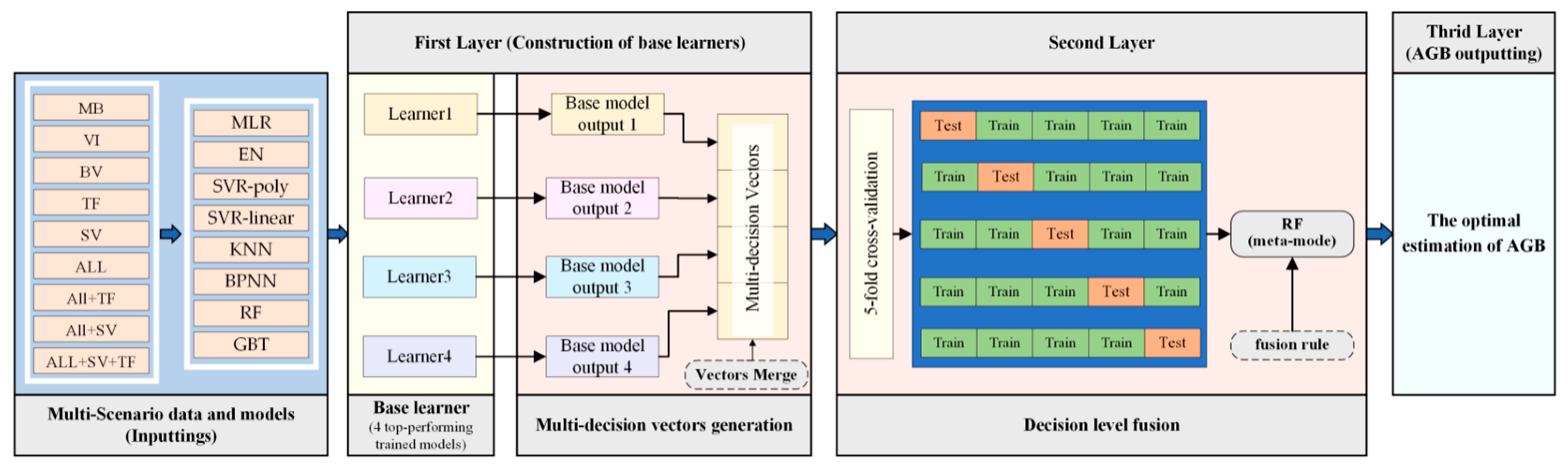
3.4. Multi-Decision Vector Fusion (MDVF) Model Construction

Due to the limitations of individual models, constructing a robust and generalizable model for a given scenario is crucial. To address this, we innovatively apply the ideas of decision-level fusion [45,46] and stacked generalization [47], typically used in classification and target detection, to AGB estimation. This study developed the MDVF model to further enhance AGB estimation performance.

Data fusion is typically categorized into pixel-level, feature-level, and decision-level fusion [48]. Pixel-level fusion occurs during preprocessing, feature-level fusion is integrated into the modeling process, and decision-level fusion operates on finalized model outputs [49,50]. Huang et al. [51] demonstrated effective decision-level fusion by combining support vector machine classification results through deterministic voting and probability weighting. In this study, we developed a three-layer MDVF model, as detailed in Figure 3. The first layer generated eight primary learners from the training features, with four top-performing models selected as base learners. In this study, RF was employed as the meta-learner in the second layer to integrate the predictions from the four base learners. RF was chosen for its ability to capture complex nonlinear relationships and its robustness against overfitting and noise. Prior studies have demonstrated that RF-based fusion methods outperform traditional parametric approaches, such as logistic regression, particularly in forest modeling tasks with heterogeneous input features [52,53,54]. The third layer, serving as the output layer, generated the fused output. To mitigate potential overfitting and multicollinearity in the second layer, five-fold cross-validation was employed, thereby enhancing the robustness and reliability of the final predictions.

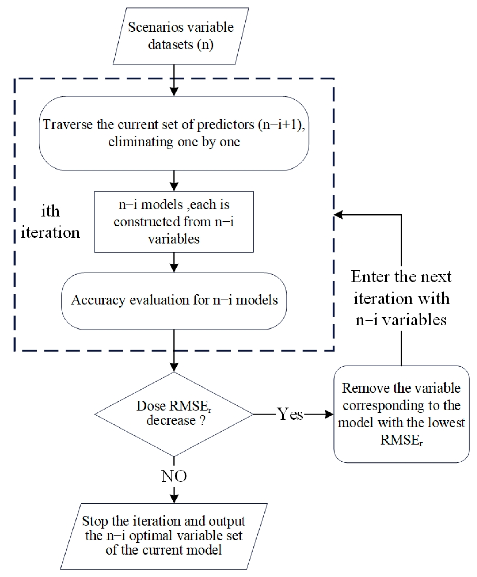
3.5. Feature Selection

Given the high dimensionality of multi-source remote sensing data and the diverse input requirements of different models, an effective, model-adaptive feature selection method is imperative. This study proposed the stepwise feature selection (SFS) method to eliminate low-performing and highly intercorrelation predictors. As shown in Figure 4, the process starts with an initial set of n variables of each experimental group (detailed in Section 3.6) for each predictive model. In each iteration, n-i models are constructed by excluding one variable at a time, and their accuracy is evaluated using RMSE_r. The variable whose exclusion results in the lowest RMSE_r is considered the least explanatory and is removed. This iterative process continues until the RMSE_r stabilizes (i.e., no longer decreases), ultimately identifying the optimal subset of predictors for each model to enhance explanatory power.

3.6. Experimental Design and Accuracy Evaluation

This study derived 36 candidate predictors from S-1 and S-2 data, including 31 optical and 5 SAR-based variables. From the AGB reference map, 750 samples were initially selected for training and validating the satellite-based AGB estimation models, with those over impervious surfaces and water bodies manually excluded using the GLC_FCS30D [23]. The final dataset comprised 708 samples, representing diverse forest types. The sample size aligns with previous studies on similar ~100 km² spatial extents [55,56]. A total of 495 samples (70%) were randomly allocated for training, while 213 samples (30%) were reserved for validation (Figure 1). The biomass values of the samples ranged from 20.36 to 269.21 Mg/ha, with a mean of 157.09 Mg/ha and a standard deviation of 52.44 Mg/ha.

To evaluate AGB estimation performance, nine experiments (hereafter “Exp.”) were conducted across eight models using different input variable combinations (see

Table 3. Experimental design of this study for AGB inversion.

Experiment	Data Scenarios	Num. 1	Data Source	Model
1	MB	10	Sentinel-2B	MLR
2	VI	10		EN
3	BV	3		SVR-poly
4	TF	8		SVR-linear
5	SV	5	Sentinel-1A	KNN
6	ALL	23	Sentinel-2B +Sentinel-1A	BPNN
7	ALL + TF	31		RF
8	ALL + SV	28		GBT
9	ALL + SV + TF	36		DMVF

¹ “Num.” represents the initial number of variables for each data scenario.

): Exp. 1: multispectral bands (MB); Exp. 2: vegetation indices (VI); Exp. 3: biophysical variables (BV); Exp. 4: texture features (TF); Exp. 5: SAR backscattering variables (SV); Exp. 6: a combination of MB, VI, and BV (ALL); Exp. 7: ALL with TF (ALL + TF); Exp. 8: ALL with SV (ALL + SV); and Exp. 9: ALL with SV and TF (ALL + SV + TF). For each model, the SFS was applied to optimize input variables. Based on the experimental results, the MDVF model was implemented for decision fusion in the final AGB estimation.

The remaining 30% of samples (213 samples) were used to evaluate the eight predictive models and the MDVF. The model accuracy was evaluated using the coefficient of determination (R²), root mean square error (RMSE, Mg/ha), and relative root mean square error (RMSE_r, %) as defined in Equations (10)–(12) to quantify the correlation and deviation between predicted and reference AGB values.

$${\mathrm{R}}^2=1-{\displaystyle \frac{{\displaystyle \sum _{i=1}^n{(X_i-Y_i)}^2}}{{\displaystyle \sum _{i=1}^n{(X_i-{\overline{Y}}_i)}^2}}}$$

(10)

$$\mathrm{RMSE}=\sqrt{{\displaystyle \frac{{\displaystyle \sum _{i=1}^n{(X_i-Y_i)}^2}}{n}}}$$

(11)

$${\mathrm{RMSE}}_{\mathrm{r}}={\displaystyle \frac{1}{{\overline{Y}}_i}}\sqrt{{\displaystyle \frac{{\displaystyle \sum _{i=1}^n{(X_i-Y_i)}^2}}{n}}}$$

(12)

where Y_i and $\overline{Y_i}$ are the AGB reference value and its mean value, respectively; X_i denotes the predicted AGB at the sampling point by ML models; and n denotes the number of validating samples.

4. Results

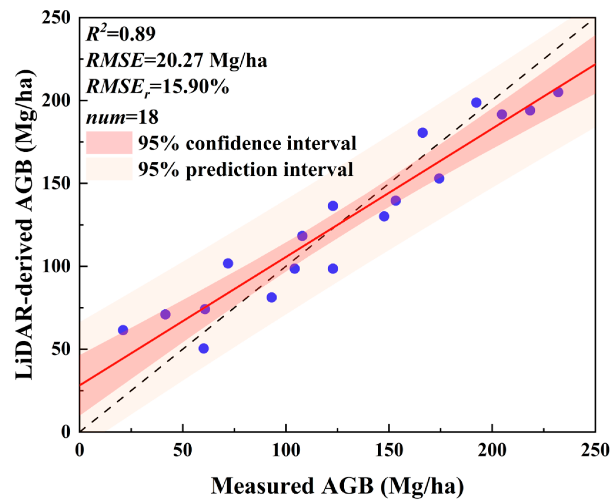
4.1. Accuracy Assessment of ABG Reference Map

Using RF-derived importance values, significant variables including H₉₅, H₉₀, H_mean, H₈₅, PD_{20_30}, CC_mean, LAD_{20_30}, H_var, H_cv, and CT were selected to construct the AGB reference map. Figure 5 shows that, in the accuracy evaluation of the AGB reference map, based on 18 field measurements, the map achieved an RMSE of 20.27 Mg/ha, R² of 0.89, and RMSE_r of 15.90%, matching or exceeding the precision reported in previous studies [57,58], which provided a reliable reference for subsequent modeling. The scatter plot in Figure 5 illustrates a strong linear correlation between the measured and LiDAR-derived AGB values, closely following the 1:1 reference line. All data points lie within the 95% prediction interval. A few points slightly deviate from the 1:1 line, particularly the underestimation of high values and the overestimation of low values, as discussed in detail in Section 5.1. The LiDAR-derived AGB values ranged from 17.87 to 275.65 Mg/ha, with an average of 127.84 Mg/ha and a standard deviation of 61.86 Mg/ha. These biomass values were then used as training and testing data for regional AGB estimation using satellite imagery.

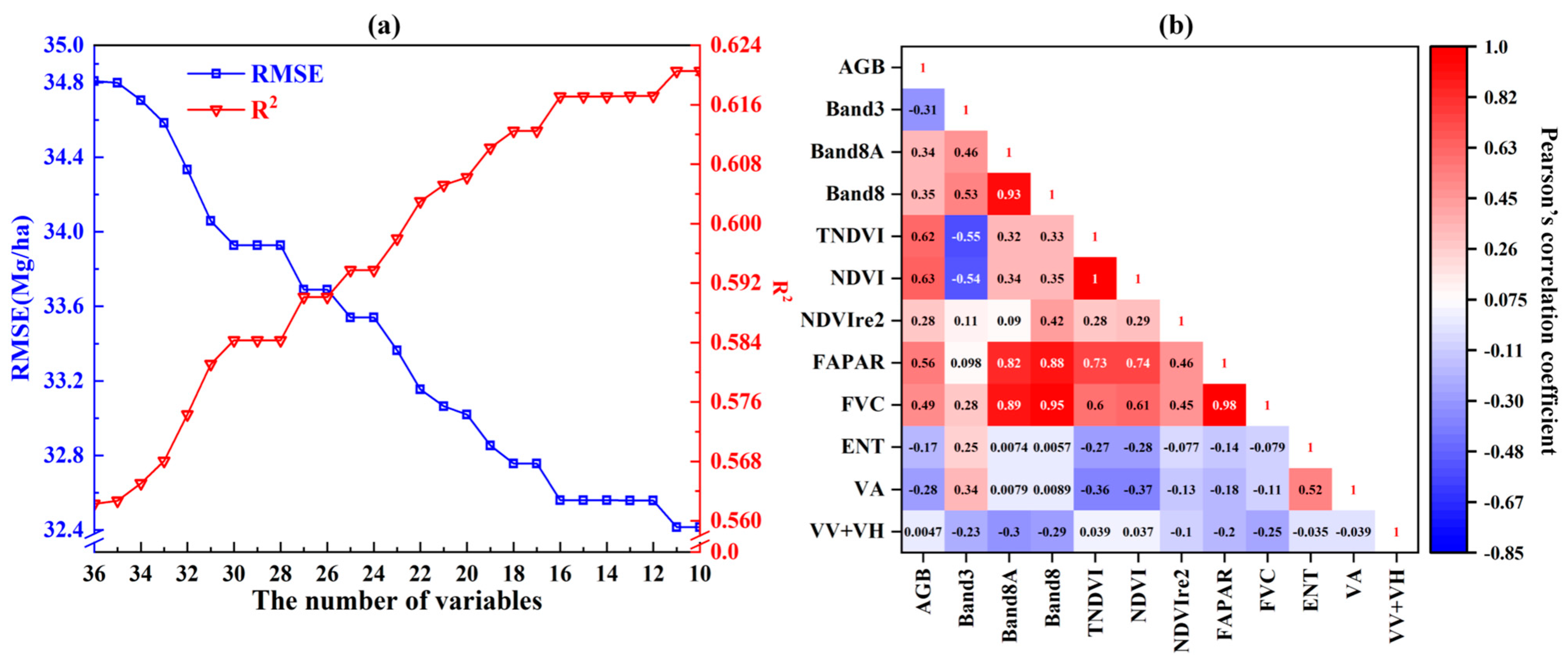
4.2. Feature Selection and First-Stage Optimization

To identify optimal predictors for each model, we conducted first-stage optimization using SFS.

Table 4. Optimal variable condition by SFS and validation accuracy of each model.

Exp. 1	MLR					EN						SVR-Linear
	Num. 2	R2		RMSE	RMSEr	Num.		R2	RMSE	RMSEr		Num.	R2	RMSE		RMSEr
1	6/10	0.568		34.592	22.7	7/10		0.562	34.811	22.8		7/10	0.577	34.220		22.4
2	8/10	0.567		34.637	22.7	8/10		0.551	35.280	23.1		9/10	0.561	34.884		22.9
3	2/3	0.496		37.367	24.5	2/3		0.497	37.334	24.5		2/3	0.454	38.881		25.5
4	4/8	0.083		50.384	33.0	4/8		0.083	50.393	33.0		5/8	0.095	50.060		32.8
5	3/5	0.067		52.819	34.6	1/5		0.029	55.935	36.7		3/5	0.032	55.238		36.2
6	10/23	0.603		33.167	21.7	10/23		0.586	33.879	22.2		5/23	0.591	33.674		22.1
7	12/31	0.604		33.106	21.7	12/31		0.586	33.842	22.2		15/31	0.593	33.591		22.0
8	11/28	0.605		33.062	21.7	12/28		0.588	33.774	22.1		12/28	0.594	33.539		22.0
9	13/36	0.607		33.006	21.6	13/36		0.589	33.738	22.1		19/36	0.595	33.508		22.0
Exp.	SVR-Poly					KNN						BPNN
	Num.	R2		RMSE	RMSEr	Num.		R2	RMSE	RMSEr		Num.	R2	RMSE		RMSEr
1	9/10	0.585		33.913	22.2	6/10		0.527	36.187	23.7		8/10	0.599	33.333		21.9
2	7/10	0.571		34.476	22.6	6/10		0.580	34.105	22.4		7/10	0.578	34.169		22.4
3	2/3	0.499		37.260	24.4	2/3		0.507	36.965	24.2		2/3	0.554	35.140		23.0
4	5/8	0.135		48.933	32.1	4/8		0.103	49.847	32.7		7/8	0.121	49.330		32.3
5	2/5	0.061		53.021	34.8	4/5		0.058	53.038	34.8		2/5	0.075	52.520		34.4
6	2/23	0.598		33.380	21.9	5/23		0.574	34.330	22.5		8/23	0.604	33.098		21.7
7	11/31	0.595		33.488	22.0	9/31		0.591	33.659	22.1		8/31	0.617	32.572		21.4
8	8/28	0.600		33.292	21.8	8/28		0.574	34.344	22.5		8/28	0.610	32.881		21.6
9	12/36	0.600		33.265	21.8	7/36		0.590	33.701	22.1		11/36	0.621	32.416		21.3
Exp.	RF								GBT
	Num.		R2		RMSE		RMSEr		Num.		R2		RMSE		RMSEr
1	3/10		0.573		34.369		22.5		5/10		0.547		35.428		23.2
2	6/10		0.566		34.664		22.7		8/10		0.589		33.725		22.1
3	2/3		0.470		38.313		25.1		2/3		0.493		37.458		24.6
4	7/8		0.125		49.227		32.3		5/8		0.113		49.561		32.5
5	2/5		0.068		52.785		34.6		2/5		0.072		52.617		34.5
6	8/23		0.604		33.097		21.7		5/23		0.598		33.372		21.9
7	11/31		0.608		0.608		21.6		6/31		0.604		33.127		21.7
8	8/28		0.600		33.279		21.8		5/28		0.603		33.176		21.7
9	12/36		0.611		32.813		21.5		19/36		0.614		32.687		21.4

¹ “Exp.” is an abbreviation for “Experiment”. ² “Num.” is the number of optimal variables extracted with the SFS method, expressed as the “optimal variable number/initial variable number of each experimental group”. The optimal set of variables identified with SFS for each model across different scenarios is detailed in Table S1 of the Supplementary.

summarizes the optimal variable sets and corresponding prediction accuracies across nine experimental scenarios.

4.2.1. Performance of Selected Predictor Sets

In the single-scenario experiments (Exp. 1–5), the MB and VI groups yielded high validation accuracies. Specifically, six models (MLR, EN, SVR-poly, SVR-linear, BPNN, and RF) performed best with MB, while KNN and GBT excelled with VI. Notably, in Exp. 1, using SFS for variable selection, the BPNN model achieved the highest single-scenario accuracy (R² of 0.599, RMSE of 33.333 Mg/ha, RMSE_r of 21.9%) using eight variables from the MB set. The BV set produced slightly lower accuracies, with R² values ranging from 0.47 to 0.554, whereas TF and SV alone resulted in poorer R² values below 0.2. However, integrating TF and SV with optical data (Exp. 7–9) improved performance, with Exp. 9 (ALL + SV + TF) yielding the best results in seven models (except KNN). Overall, the synergy of optical and SAR data, along with texture features, reduced the RMSE_r by up to ~2.05% compared to using optical variables alone.

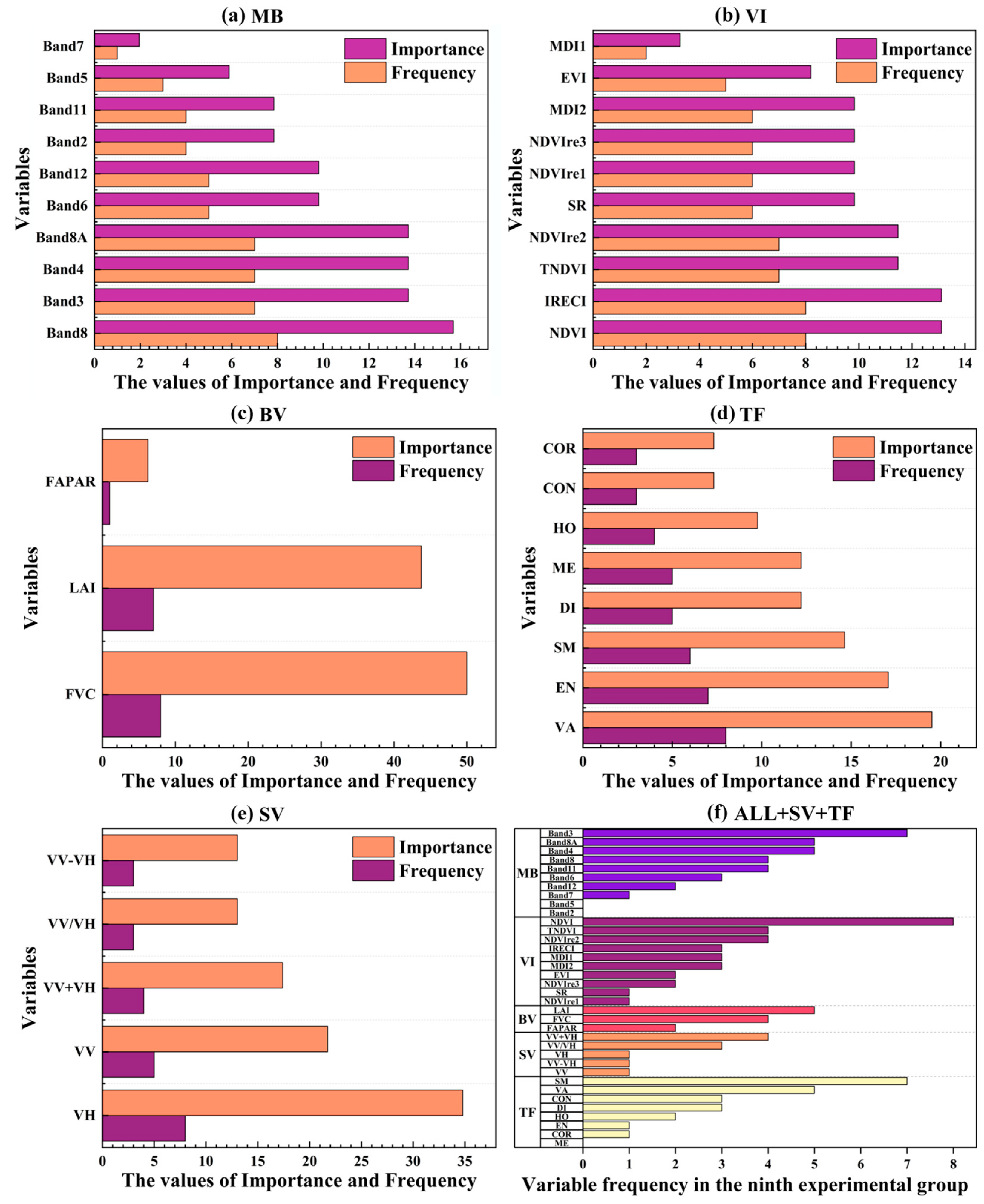
4.2.2. Key Variables Adaptively Identified by SFS

SFS was used to adaptively select optimal input predictors for different models. Variable importance was quantified as the ratio of the frequency with which a specific variable was selected to the total number of variable selections across all models in each scenario. The importance of variables in the single-scenario experiments (Exp. 1–5) and the ALL + SV + TF scenario (Exp. 9) is illustrated in Figure 6. In the MB set, Band8, Band3, Band4, and Band8A were frequently used, with Band8 (NIR) chosen by all eight models. For VI, all indices except MDI1 were selected by more than half the models, with NDVI and IRECI chosen by all. In the BV, TF, and SV groups, FVC, VA, and VH emerged as key factors with importance values of 50%, 19.51%, and 34.75%, respectively.

In the ALL + SV + TF set, inter-variable interactions may affect the significance of predictors. Figure 6f shows that, despite slight deviations from single-scenario selections, key variables remain consistently chosen. Notably, Band3, NDVI, LAI, SM, and VV + VH were the most frequently selected, consistently ranking among the top three in Exp. 1–5.

4.2.3. Model Performance with Optimal Feature Set

Table 4 shows that among the eight models, BPNN outperformed the others, with an accuracy ranking of BPNN > GBT > RF > MLR > SVR-poly > SVR-linear > KNN > EN (Exp. 9). Using 11 variables from the ALL + SV + TF set, BPNN achieved an R² of 0.621, RMSE of 32.416 Mg/ha, and RMSE_r of 21.3%. In general, non-parametric models outperformed parametric ones, with BPNN achieving a 3.92% increase in RMSE_r compared to EN; nonlinear models yielded higher accuracies than linear counterparts, with SVR-poly showing an RMSE_r increase of 0.72% compared to SVR-linear.

4.3. Hyperparameter Tuning and Second-Stage Optimization

In Exp. 9 (ALL + SV + TF), all eight predictive models, except for KNN, outperformed the other scenarios. A grid search strategy was then applied to optimize key hyperparameters for these models while maintaining computational efficiency.

Table 5. Results of optimized parameters for eight models.

Model	Data Scenario	Optimized Parameter	R2	RMSE	RMSEr
BPNN	ALL + SV + TF	max_iter = 135, activation function = logistic sigmoid, solver = stochastic gradient descent, learning rate = 0.0013, hidden_layer_sizes = 100, Alpha = 2.02	0.625	32.207	21.1
GBT	ALL + SV + TF	Ntree = 105, max_depth = 2, min_samples_leaf = 2, min_samples_split = 6, learning rate = 0.09, subsampling rate = 0.98	0.617	32.568	21.4
RF	ALL + SV + TF	Ntree = 350, max_depth = 16, min_samples_leaf = 1, min_samples_split = 3	0.613	32.715	21.4
MLR	ALL + SV + TF	None	0.607	33.006	21.6
SVR-poly	ALL + SV + TF	C = 1.5, epsilon = 4.5, d = 3, r = 2	0.606	33.031	21.7
KNN	ALL + TF	k = 15, distance function = manhattan_distance	0.601	33.244	21.8
SVR-linear	ALL + SV + TF	C = 5.5, epsilon = 0.002	0.599	33.311	21.8
EN	ALL + SV + TF	α = 0.1, ρ = 1, max_iter = 500	0.595	33.496	22.0

Note: The bold type indicates the accuracy of the four top-performing models.

details the optimized parameters, with the BPNN achieving the highest accuracy (R² = 0.625, RMSE = 32.207 Mg/ha, RMSE_r = 21.1%), followed by GBT (R² = 0.617, RMSE = 32.568 Mg/ha, RMSE_r = 21.4%) and RF (R² = 0.613, RMSE = 32.715 Mg/ha, RMSE_r = 21.4%). Other models ranked as follows in accuracy: MLR, SVR-poly, KNN, SVR-linear, EN. Figure 7 displays the validation scatter plots, where the linear fit for BPNN is closest to the 1:1 line, exhibiting the smallest residuals. Moreover, as shown in Figure 8a, all models exhibited modest accuracy improvements after second-stage optimization, with KNN demonstrating the largest improvement (a 1.7% increase in R² and a 1.23% decrease in RMSE). Notably, the four top-performing models consistently performed well across the second optimization rounds, with BPNN, GBT, and RF showing minor R² increases of 0.79%, 0.46%, and 0.38%, respectively. However, MLR did not require further hyperparameter optimization.

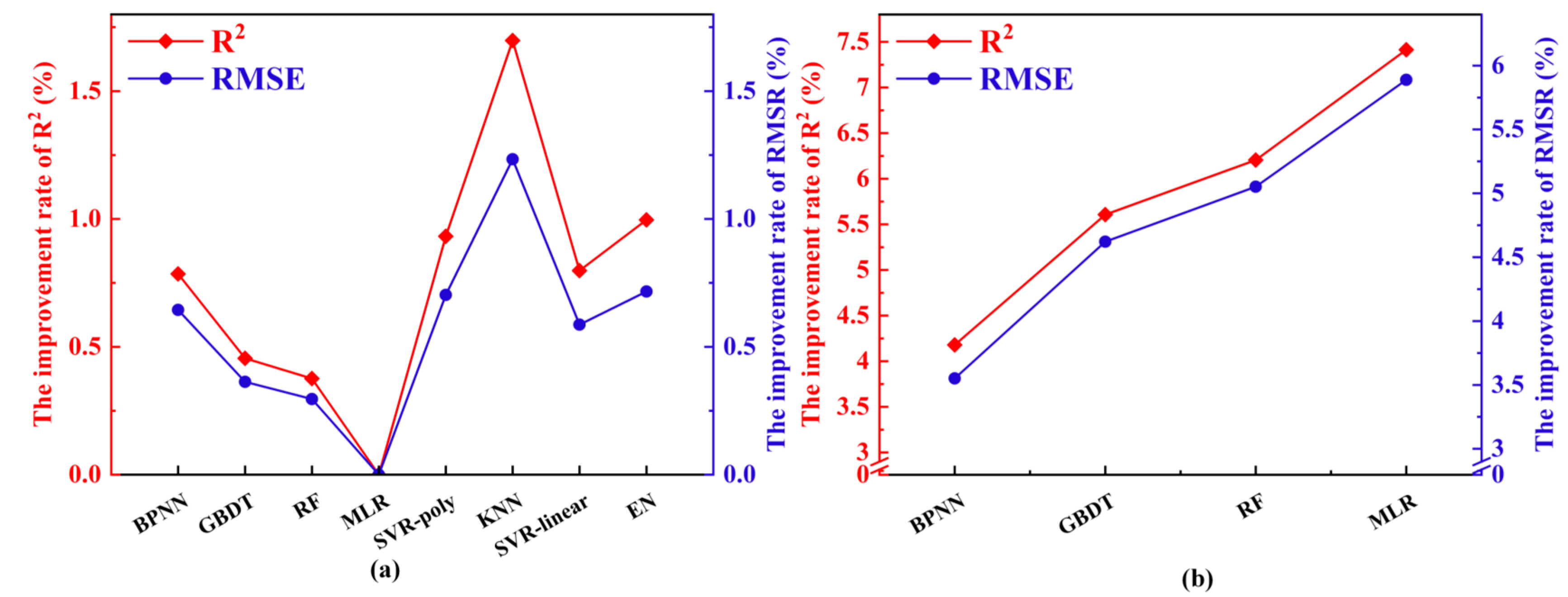
4.4. MDVF Performance and Third-Stage Optimization

To further improve AGB estimation, the MDVF model was developed by fusing the four best-performing models (BPNN, GBT, RF, and MLR) from the second-stage optimization, using RF as the fusion rule. Hyperparameters for the fusion rule were set to Ntree = 30, Max_depth = 12, min_samples_split = 8, and min_samples_leaf = 2. Based on inputs from Exp. 9 (ALL + SV + TF),

Table 6. Parameter settings of meta-learner (random forest, RF) and accuracy results of the MDVF model.

Data Scenarios	Num. 1	Optimal Variables	Parameters of RF	R2	RMSE	RMSEr
ALL + SV + TF	21/36	Band2, Band3, Band5, Band6, Band7, Band8a, Band11, Band12, TNDVI, EVI, NDVIre3, MDI1, LAI, DIS, EN COR, ME, VA, VV + VH, VV − VH, VV	Ntree = 30 max_depth = 12 min_samples_split = 8 min_samples_leaf = 2	0.652	31.063	20.4

¹ “Num.” is the number of optimal variables extracted with the SFS method, expressed as the “optimal variable number/initial variable number of each experimental group”.

summarizes the variable selection, parameter optimization, and accuracy of the MDVF. Compared to previous studies in subtropical forests in China, our approach demonstrates enhanced accuracy in AGB estimation. For example, Pan et al. [59] utilized S-1 and S-2 data, combined with linear regression modeling, to estimate the AGB of fir forests in the subtropical region of China. Their study achieved an R² of 0.575 and an RMSE of 59.13 Mg/ha. In contrast, our study employed ML techniques within the MDVF, resulting in an R² of 0.652 and an RMSE of 31.063 Mg/ha, indicating a significant improvement in estimation accuracy. Additionally, the AGB estimated using MDVF showed a significant improvement in accuracy compared to the base learners, whose RMSE values ranged from 32.21 to 33.01 Mg/ha for BPNN, GBT, RF, and MLR (more detailed accuracy metrics are highlighted in bold in Table 5). As illustrated in Figure 9, MDVF predictions are more tightly clustered around the 1:1 line and converge better within the 95% prediction band compared to the models after the second-stage optimization (see Figure 7).

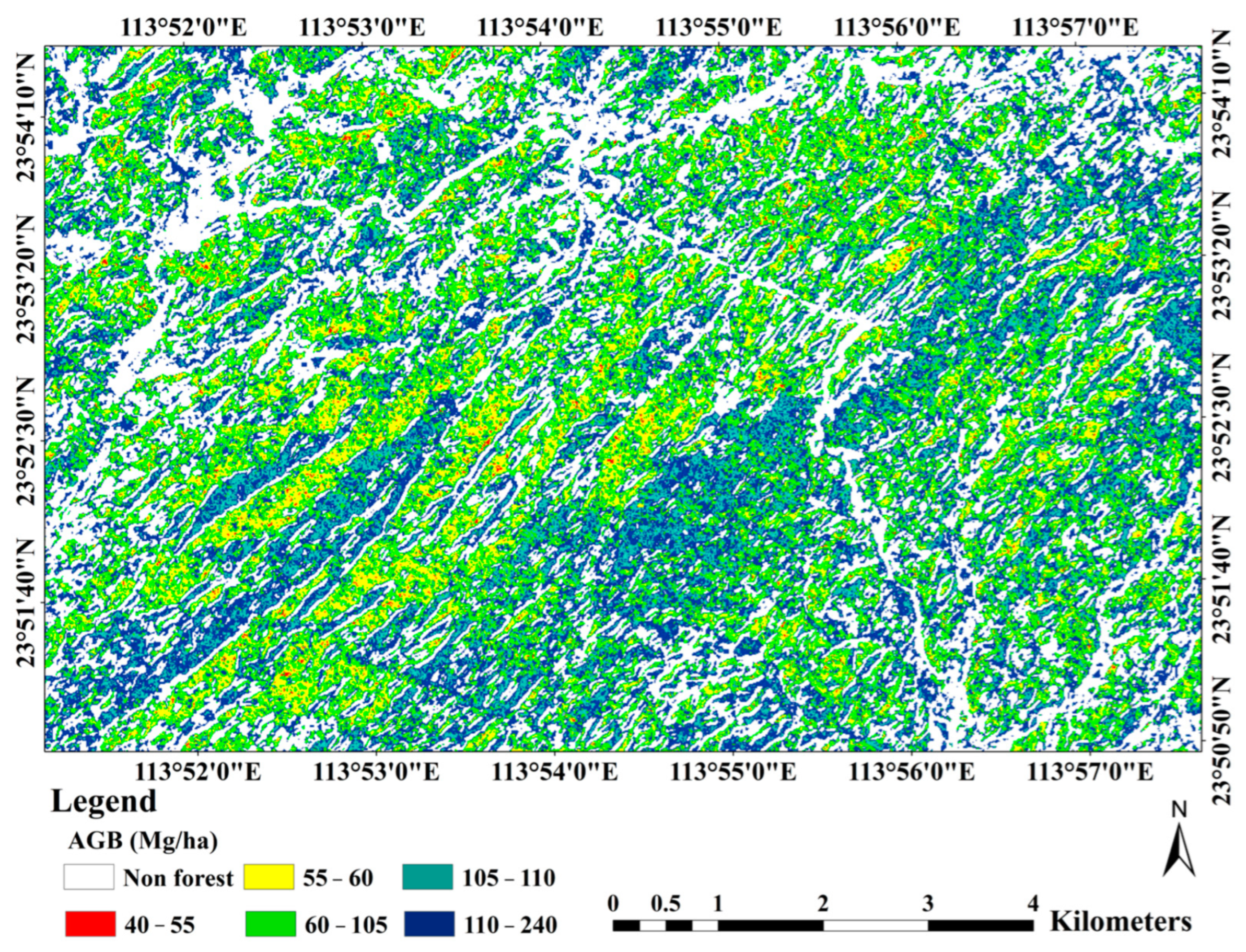
4.5. Forest AGB Mapping and Spatial Distribution Analysis

Figure 10 presents the AGB predictions for the study area using the MDVF model, with values ranging from 39.37 to 239.03 Mg/ha and an average of 102.17 Mg/ha. Non-forest areas such as impervious surfaces, buildings, clouds, and water bodies were excluded. The central region exhibited lower AGB values, whereas the southeast had higher values. Approximately 70% of the biomass values fell within the 55–110 Mg/ha range, representing the majority of the effective pixels.

5. Discussion

5.1. LiDAR-Derived AGB as a Reliable Reference for Estimation

This study confirms that LiDAR-derived metrics serve as an efficient and reliable supplement to traditional forest inventories for estimating forest AGB, particularly in subtropical forest regions where field surveys are challenging to conduct. Prior research has validated the effectiveness of discrete-return, small-footprint LiDAR in AGB estimation [60]. Among the LiDAR-derived features selected via RF, key predictors such as P₉₅, P₉₀, H_mean, and LAD_{20_30} were identified, aligning with findings from similar studies [52]. The validation results (Figure 5) demonstrate the strong predictive capability of the selected features. However, a systematic bias is observed, with slight underestimation at high biomass levels and overestimation at low levels. The former is primarily caused by signal saturation in dense canopies, while the latter may result from background spectral interference [61], increased noise in sparse canopies [62], incomplete ground–vegetation separation [63], and the limited vertical resolution of LiDAR systems [64].

In this study, airborne LiDAR data provided full coverage of the ~100 km² study area, allowing for the generation of a spatially continuous and high-accuracy AGB reference map. While this was feasible due to the limited extent of the study region, in practice, airborne LiDAR data are typically acquired as discrete flight strips, and field plots are often sparse and unevenly distributed in larger-scale applications. Thus, we developed a two-step framework: field measurements were first used to train the LiDAR-based AGB model, producing a reliable reference map, which was then used to train satellite-based models for large-scale AGB mapping. This approach aligns with recent studies using LiDAR-derived maps as an intermediate source to upscale plot-level measurements in data-scarce tropical forests [65]. As shown in Section 4.4, the satellite-based estimates achieved accuracy comparable to that of LiDAR-only model, demonstrating the method’s effectiveness for forest AGB mapping where field or LiDAR data are limited.

Additionally, geolocation errors in LiDAR data, typically within a few meters depending on sensor and platform configurations, may cause spatial misalignments with field plots and satellite data, potentially impacting AGB estimation. Although not the central focus of this study, such effects were mitigated by selecting 30 m plots located in areas with generally homogeneous canopies and by integrating multi-source data and models. Previous studies have shown that larger plots (e.g., 10 m radius) reduce co-registration errors and edge effects in LiDAR-based biomass estimation, particularly in structurally complex subtropical forests [66]. The high validation accuracy of both the LiDAR-based reference model and subsequent satellite-based AGB estimates indicates that these residual uncertainties were effectively controlled. Nonetheless, further research is needed to better quantify and minimize spatial misalignment in future applications.

5.2. Contribution of Multi-Source Data to AGB Estimation

This study assessed the performance of active and passive remote sensing data across nine modeling scenarios. The results show that S-2 outperformed S-1 in AGB retrieval, consistent with Forkuor et al. [67], but contrasting with Georgopoulos et al. [68]. The limited penetration capability of S-1’s C-band (5.7 GHz) SAR through dense canopies leads to signal saturation around 60–70 Mg/ha, as noted by Nizalapur et al. [69]. Given that most plots in the study area exceeded this extent, models relying on S-1 alone performed poorly. The humid subtropical climate of Conghua District further exacerbates these limitations. High canopy moisture increases the dielectric constant of vegetation, enhancing volume scattering and also increasing attenuation, especially in dense forests. In high-biomass areas, reduced signal penetration and multiple scattering effects lead to saturation, reducing the sensitivity of C-band SAR to biomass variations [63]. In contrast, high soil moisture under sparse canopies amplifies surface scattering, potentially resulting in biomass overestimation [70]. Together, these factors limit the reliability of using C-band SAR alone for AGB estimation in humid subtropical forests.

S-2 optical data, enriched with vegetation indices and biophysical variables, significantly contribute to AGB modeling. Notably, despite comprising only three variables, the BV group achieved approximately 87% of the explanatory capacity (assessed by R²) of the MB and VI groups, each containing 10 variables. In Exp. 9, LAI and FVC from the BV group were selected by over half of the models, underscoring the value of S-2-derived biophysical variables in AGB prediction. Additionally, spectral-derived texture features from PCA1 alone did not produce satisfactory AGB estimates because they primarily capture horizontal canopy structures, which tend to saturate in dense forests. As Zhao et al. [71] noted, texture feature performance varies with remote sensing data and vegetation type. It is recommended to integrate the structural information provided by SAR and texture variables with conventional spectral bands and vegetation indices to effectively mitigate saturation effects in dense vegetation, thereby enhancing AGB estimation (see Table 6).

In the multi-scenario groups, the ALL scenario (combining MB, VI, and BV) outperformed individual groups in validation accuracy. Further, Exp. 9 (ALL + SV + TF) showed that the inclusion of optical texture and SAR features improved R² by an average of 1.5% across eight predictive models. This enhancement reflects the complementary strengths of active and passive remote sensing data. Optical sensors capture spectral characteristics and horizontal structure, while SAR provides insights into vertical structure and moisture content, thereby significantly improving AGB estimation accuracy.

5.3. Effectiveness of Stepwise Feature Selection Method

This study employed a model-adaptive feature selection method to reduce variable redundancy and improve model performance. As shown in Figure 11a, the validation accuracy of BPNN in Exp. 9 improved as irrelevant and low-explanatory predictors were eliminated from an initial set of 36 variables, resulting in a 10.28% increase in R² and a 6.85% decrease in RMSE. Notably, reducing the set below 11 variables did not further enhance accuracy, indicating that too few predictors compromise optimal AGB estimation. The average discard rates for individual variable groups were 36% (MB), 26% (VI), 33% (BV), 36% (TF), and 53% (SV), while combined scenarios exhibited discard rates ranging from 63% to 71%. These results highlight that the SFS method, through feature combination and stepwise selection, effectively minimizes redundancy and autocorrelation, enhancing computational efficiency and prediction accuracy.

Figure 11b presents heatmaps for the BPNN model using the optimal variable set identified through SFS in Exp. 9. According to the interpretation of Pearson’s correlation coefficient (PCC) by Mukaka [72], none of the 11 optimal variables showed a strong correlation (PCC > 0.7) with AGB; only 4 exhibited moderate correlations (0.4 < PCC < 0.69), with the remainder demonstrating weak correlations (0 < PCC < 0.39). This weak linear association underscores the limitations of relying solely on linear correlation for variable selection and validates the necessity of the SFS approach. Furthermore, 43.64% of the selected variables had weak correlations, and 21.82% showed negligible correlations, demonstrating SFS’s ability to reduce multicollinearity and enhance feature selection effectiveness. Despite the absence of strong linear relationships, these variables yielded the most accurate estimate in the first optimization round, emphasizing the effectiveness of SFS in identifying optimal predictors.

5.4. Model Comparisons and the Impact of Hyperparameter Optimization

In this study, a grid search strategy was employed to optimize hyperparameters for each model, enhancing AGB estimation accuracy while maintaining computational efficiency. As detailed in Table 6, non-parametric machine learning models, particularly BPNN, outperformed parametric methods, achieving an R² of 0.625, RMSE of 32.207 Mg/ha, and RMSE_r of 21.1%. DT-based ensemble models, including GBT and RF, also demonstrated strong performance. These reflect the advantage of multidimensional network architectures and ensemble methods in capturing complex nonlinear relationships between AGB and remote sensing variables.

Hyperparameter selection plays a critical role in model generalization. Excessively high values for max_iter in BPNN or Ntree in RF can lead to overfitting, as models adjust weights iteratively to minimize residual errors, potentially capturing noise rather than meaningful patterns. To balance accuracy and generalization, max_iter for BPNN was finally optimized to 135, and Ntree for RF was set to 350, both aligning with effective parameter ranges reported in previous AGB estimation studies [73,74].

5.5. MDVF Performance and the Advantages of Three-Stage Optimization

In this study, we developed the MDVF model to implement third-stage optimization for forest AGB estimation, using RF as the meta-learner to integrate outputs from the top-performing base models. Unlike traditional decision-level fusion methods with static weights, RF adaptively assigns weights based on data characteristics, reducing overfitting and enhancing model robustness. Previous studies have demonstrated the superiority of RF-based stacking over single-model and parametric fusion approaches in complex forest parameter modeling. For instance, Healey et al. [54] reported reduced omission and commission errors with RF-based ensembles, while Araza et al. [75] confirmed the effectiveness of RF-based fusion rule in capturing spatial heterogeneity in large-scale carbon flux mapping. Our selection of RF aligns with these established findings and substantially improves both the accuracy and generalization of AGB predictions. Furthermore, five-fold cross-validation combined with the out-of-bag error estimation further stabilized the meta-model performance.

This study implemented a three-stage optimization strategy to achieve highly precise AGB estimation. At the first stage, using BPNN as an example, the feature selection with SFS enhanced the R² of BPNN by 10.28% and reduced the RMSE by 6.85% in Exp. 9 (see Figure 11a). As shown in Table 4, the synergy of active and passive remote sensing variables in Exp. 9 increased R² by 3.64% and decreased RMSE by 2.64%, compared to using only spectral data in Exp. 1. However, the hyperparameter tuning at the second stage yielded less than 2% accuracy improvement (see Figure 8a). In contrast, decision-level fusion via MDVF in the third stage improved R² by an average of 5.85% and reduced RMSE by an average of 4.78% compared to the base models (see Figure 8b). These results indicate that data synergy, adaptive variable selection, and model fusion significantly enhance AGB estimation accuracy, whereas extensive hyperparameter tuning offers only marginal benefits. This underscores the necessity of integrating active and passive remote sensing data and prioritizing model fusion strategies over computationally intensive parameter optimization.

6. Conclusions

This study proposed a multi-source data synergy framework for forest aboveground biomass (AGB) estimation by integrating (Sentinel-1) S-1 and (Sentinel-2) S-2 data with a LiDAR-derived reference map. A three-stage optimization strategy was employed, including stepwise variable selection, hyperparameter optimization, and multi-decision vector fusion (MDVF). The key findings are as follows:

(1) Discrete-return small-footprint LiDAR accurately estimated forest AGB and served as a reliable supplement to traditional forest inventories, providing a means to scale up field-based measurements in data-scarce regions.

(2) Effective variable selection is crucial when modeling with multi-dimensional remote sensing data. SFS effectively reduced variable redundancy and multicollinearity, enhancing the accuracy and efficiency of multi-source AGB modeling.

(3) The NIR from S-2, along with vegetation indices (especially NDVI and the RE band-derived vegetation index like IRECI) and biophysical variables (especially the LAI), were highly effective for AGB prediction. While C-band SAR variables from S-1 and texture features derived from S-2 alone underperform in sparse and dense vegetation, integrating them as auxiliary predictors mitigated saturation effects in optical data.

(4) Non-parametric and nonlinear machine learning models, particularly BPNN, RF, and GBT, outperformed parametric approaches by effectively capturing the complex relationships between AGB and remote sensing features.

(5) DMVF was proposed in forest AGB mapping for the first time, achieving superior performance (R² = 0.652, RMSE = 31.063 Mg/ha, RMSE_r = 20.4%) by integrating multiple ML algorithms with RF as the fusion rule. It effectively captured nonlinear relationships between features and AGB, demonstrating greater robustness and predictive accuracy than any single model (with R² increasing by 4.18–7.41% and RMSE decreasing by 3.55–5.89% compared to the four top-performing models in the second optimization stage). These findings highlight DMVF’s potential for broader applications in forest biophysical parameter inversion.

(6) The synergy of active and passive data, effective variable selection, and model fusion significantly enhance AGB estimation, proving more crucial than extensive hyperparameter tuning.

Overall, this study demonstrates the potential of integrating LiDAR-derived AGB reference data with synergistic active SAR and passive optical remote sensing observations for large-scale, high-precision AGB mapping. The proposed three-stage optimization scheme and MDVF model provide a cost-effective, precise and scalable solution for forest resource monitoring and carbon stock assessments.

References

1. Bonan, G.B. Forests and climate change: Forcings, feedbacks, and the climate benefits of forests. Science 2008, 320, 1444–1449. [Google Scholar] [CrossRef]
2. Yang, K.; Zhang, Q.; Zhu, J.J.; Wang, Q.Q.; Gao, T.; Wang, G.G. Mycorrhizal type regulates trade-offs between plant and soil carbon in forests. Nat. Clim. Change 2023, 13, 1279–1281. [Google Scholar] [CrossRef]
3. Heimann, M.; Reichstein, M. Terrestrial ecosystem carbon dynamics and climate feedbacks. Nature 2008, 451, 289–292. [Google Scholar] [CrossRef]
4. Quegan, S.; Toan, L.T.; Chave, J.; Dall, J.; Exbrayat, J.F.; Minh, D.H.T.; Lomas, M.; D’Alessandro, M.M.; Paillou, P.; Papathanassiou, K.; et al. The European Space Agency BIOMASS mission: Measuring forest above-ground biomass from space. Remote Sens. Environ. 2019, 227, 44–60. [Google Scholar] [CrossRef]
5. Pan, Y.D.; Birdsey, R.A.; Fang, J.Y.; Houghton, R.; Kauppi, P.E.; Kurz, W.A.; Phillips, O.L.; Shvidenko, A.; Lewis, S.L.; Canadell, J.G.; et al. A Large and Persistent Carbon Sink in the World’s Forests. Science 2011, 333, 988–993. [Google Scholar] [CrossRef] [PubMed]
6. Su, Y.J.; Guo, Q.H.; Xue, B.L.; Hu, T.Y.; Alvarez, O.; Tao, S.L.; Fang, J.Y. Spatial distribution of forest aboveground biomass in China: Estimation through combination of spaceborne lidar, optical imagery, and forest inventory data. Remote Sens. Environ. 2016, 173, 187–199. [Google Scholar] [CrossRef]
7. Clark, D.B.; Kellner, J.R. Tropical forest biomass estimation and the fallacy of misplaced concreteness. J. Veg. Sci. 2012, 23, 1191–1196. [Google Scholar] [CrossRef]
8. Zheng, D.L.; Rademacher, J.; Chen, J.Q.; Crow, T.; Bresee, M.; le Moine, J.; Ryu, S.R. Estimating aboveground biomass using Landsat 7 ETM+ data across a managed landscape in northern Wisconsin, USA. Remote Sens. Environ. 2004, 93, 402–411. [Google Scholar] [CrossRef]
9. Wittke, S.; Yu, X.; Karjalainen, M.; Hyyppa, J.; Puttonen, E. Comparison of two-dimensional multitemporal Sentinel-2 data with three-dimensional remote sensing data sources for forest inventory parameter estimation over a boreal forest. Int. J. Appl. Earth Obs. Geoinf. 2019, 76, 167–178. [Google Scholar] [CrossRef]
10. Ramos Vieira Martins, F.d.S.; dos Santos, J.R.; Galvao, L.S.; Magalhaes Xaud, H.A. Sensitivity of ALOS/PALSAR imagery to forest degradation by fire in northern Amazon. Int. J. Appl. Earth Obs. Geoinf. 2016, 49, 163–174. [Google Scholar] [CrossRef]
11. Maimaitijiang, M.; Ghulam, A.; Sidike, P.; Hartling, S.; Maimaitiyiming, M.; Peterson, K.; Shavers, E.; Fishman, J.; Peterson, J.; Kadam, S.; et al. Unmanned Aerial System (UAS)-based phenotyping of soybean using multi-sensor data fusion and extreme learning machine. ISPRS J. Photogramm. Remote Sens. 2017, 134, 43–58. [Google Scholar] [CrossRef]
12. Stelmaszczuk-Górska, M.; Urbazaev, M.; Schmullius, C.; Thiel, C. Estimation of Above-Ground Biomass over Boreal Forests on Siberia Using Updated In Situ, ALOS-2 PALSAR-2, and RADARSAT-2 Data. Remote Sens. 2018, 10, 1550. [Google Scholar] [CrossRef]
13. Tsui, O.W.; Coops, N.C.; Wulder, M.A.; Marshall, P.L.; McCardle, A. Using multi-frequency radar and discrete-return LiDAR measurements to estimate above-ground biomass and biomass components in a coastal temperate forest. ISPRS J. Photogramm. Remote Sens. 2012, 69, 121–133. [Google Scholar] [CrossRef]
14. Hafner, S.; Ban, Y.F.; Nascetti, A. Unsupervised domain adaptation for global urban extraction using Sentinel-1 SAR and Sentinel-2 MSI data. Remote Sens. Environ. 2022, 280, 113192. [Google Scholar] [CrossRef]
15. Tian, X.; Su, Z.; Chen, E.; Li, Z.; van der Tol, C.; Guo, J.; He, Q. Reprint of: Estimation of forest above-ground biomass using multi-parameter remote sensing data over a cold and arid area. Int. J. Appl. Earth Obs. Geoinf. 2012, 17, 102–110. [Google Scholar] [CrossRef]
16. Khosravipour, A.; Skidmore, A.K.; Wang, T.J.; Isenburg, M.; Khoshelham, K. Effect of slope on treetop detection using a LiDAR Canopy Height Model. ISPRS J. Photogramm. Remote Sens. 2015, 104, 44–52. [Google Scholar] [CrossRef]
17. Falkowski, M.J.; Evans, J.S.; Martinuzzi, S.; Gessler, P.E.; Hudak, A.T. Characterizing forest succession with lidar data: An evaluation for the Inland Northwest, USA. Remote Sens. Environ. 2009, 113, 946–956. [Google Scholar] [CrossRef]
18. Chirici, G.; Giannetti, F.; McRoberts, R.E.; Travaglini, D.; Pecchi, M.; Maselli, F.; Chiesi, M.; Corona, P. Wall-to-wall spatial prediction of growing stock volume based on Italian National Forest Inventory plots and remotely sensed data. Int. J. Appl. Earth Obs. Geoinf. 2020, 84, 101959. [Google Scholar] [CrossRef]
19. Moghaddam, S.H.A.; Mokhtarzade, M.; Beirami, B.A. A feature extraction method based on spectral segmentation and integration of hyperspectral images. Int. J. Appl. Earth Obs. Geoinf. 2020, 89, 102097. [Google Scholar] [CrossRef]
20. Li, W.; Niu, Z.; Shang, R.; Qin, Y.; Wang, L.; Chen, H. High-resolution mapping of forest canopy height using machine learning by coupling ICESat-2 LiDAR with Sentinel-1, Sentinel-2 and Landsat-8 data. Int. J. Appl. Earth Obs. Geoinf. 2020, 92, 102163. [Google Scholar] [CrossRef]
21. Liu, Y.; Gong, W.; Xing, Y.; Hu, X.; Gong, J. Estimation of the forest stand mean height and aboveground biomass in Northeast China using SAR Sentinel-1B, multispectral Sentinel-2A, and DEM imagery. ISPRS J. Photogramm. Remote Sens. 2019, 151, 277–289. [Google Scholar] [CrossRef]
22. Zhao, J.; Zhang, C.; Min, L.; Guo, Z.; Li, N. Retrieval of Farmland Surface Soil Moisture Based on Feature Optimization and Machine Learning. Remote Sens. 2022, 14, 5102. [Google Scholar] [CrossRef]
23. Zhang, X.; Zhao, T.T.; Xu, H.; Liu, W.D.; Wang, J.Q.; Chen, X.D.; Liu, L.Y. GLC_FCS30D: The first global 30 m land-cover dynamics monitoring product with a fine classification system for the period from 1985 to 2022 generated using dense-time-series Landsat imagery and the continuous change-detection method. Earth Syst. Sci. Data 2024, 16, 1353–1381. [Google Scholar] [CrossRef]
24. Godwin, C.; Chen, G.; Singh, K.K. The impact of urban residential development patterns on forest carbon density: An integration of LiDAR, aerial photography and field mensuration. Landsc. Urban Plan. 2015, 136, 97–109. [Google Scholar] [CrossRef]
25. Fang, J.; Liu, G.; Xu, S. Biomass and Net Production of Forest Vegetation in China. Acta Ecol. Sin. 1996, 16, 497–508. [Google Scholar]
26. ESA. Sentinel Application Platform (SNAP), ver. 9.0.0. European Space Agency: Paris, France, 2022. Available online: https://step.esa.int/main/download/snap-download/ (accessed on 7 July 2024).
27. Warmerdam, F. The geospatial data abstraction library. In Open Source Approaches in Spatial Data Handling; Springer: Berlin/Heidelberg, Germany, 2008; pp. 87–104. [Google Scholar]
28. Zhu, X.; Skidmore, A.K.; Darvishzadeh, R.; Wang, T. Estimation of forest leaf water content through inversion of a radiative transfer model from LiDAR and hyperspectral data. Int. J. Appl. Earth Obs. Geoinf. 2019, 74, 120–129. [Google Scholar] [CrossRef]
29. Majasalmi, T.; Rautiainen, M. The potential of Sentinel-2 data for estimating biophysical variables in a boreal forest: A simulation study. Remote Sens. Lett. 2016, 7, 427–436. [Google Scholar] [CrossRef]
30. Murray, H.; Lucieer, A.; Williams, R. Texture-based classification of sub-Antarctic vegetation communities on Heard Island. Int. J. Appl. Earth Obs. Geoinf. 2010, 12, 138–149. [Google Scholar] [CrossRef]
31. Dube, T.; Mutanga, O. Investigating the robustness of the new Landsat-8 Operational Land Imager derived texture metrics in estimating plantation forest aboveground biomass in resource constrained areas. ISPRS J. Photogramm. Remote Sens. 2015, 108, 12–32. [Google Scholar] [CrossRef]
32. Hudak, A.T.; Strand, E.K.; Vierling, L.A.; Byrne, J.C.; Eitel, J.U.H.; Martinuzzi, S.; Falkowski, M.J. Quantifying aboveground forest carbon pools and fluxes from repeat LiDAR surveys. Remote Sens. Environ. 2012, 123, 25–40. [Google Scholar] [CrossRef]
33. Li, Y.; Chen, R.; He, B.; Veraverbeke, S. Forest foliage fuel load estimation from multi-sensor spatiotemporal features. Int. J. Appl. Earth Obs. Geoinf. 2022, 115, 103101. [Google Scholar] [CrossRef]
34. Were, K.; Bui, D.T.; Dick, O.B.; Singh, B.R. A comparative assessment of support vector regression, artificial neural networks, and random forests for predicting and mapping soil organic carbon stocks across an Afromontane landscape. Ecol. Indic. 2015, 52, 394–403. [Google Scholar] [CrossRef]
35. Pedregosa, F.; Varoquaux, G.; Gramfort, A.; Michel, V.; Thirion, B.; Grisel, O.; Blondel, M.; Prettenhofer, P.; Weiss, R.; Dubourg, V.; et al. Scikit-learn: Machine Learning in Python. J. Mach. Learn. Res. 2011, 12, 2825–2830. [Google Scholar]
36. Chen, L.; Ren, C.; Zhang, B.; Wang, Z.; Xi, Y. Estimation of Forest Above-Ground Biomass by Geographically Weighted Regression and Machine Learning with Sentinel Imagery. Forests 2018, 9, 582. [Google Scholar] [CrossRef]
37. Wang, L.a.; Zhou, X.; Zhu, X.; Dong, Z.; Guo, W. Estimation of biomass in wheat using random forest regression algorithm and remote sensing data. Crop J. 2016, 4, 212–219. [Google Scholar] [CrossRef]
38. Heiskanen, J.; Rautiainen, M.; Korhonen, L.; Mottus, M.; Stenberg, P. Retrieval of boreal forest LAI using a forest reflectance model and empirical regressions. Int. J. Appl. Earth Obs. Geoinf. 2011, 13, 595–606. [Google Scholar] [CrossRef]
39. Lu, D.; Chen, Q.; Wang, G.; Liu, L.; Li, G.; Moran, E. A survey of remote sensing-based aboveground biomass estimation methods in forest ecosystems. Int. J. Digit. Earth 2016, 9, 63–105. [Google Scholar] [CrossRef]
40. Jiang, F.; Sun, H.; Chen, E.; Wang, T.; Cao, Y.; Liu, Q. Above-Ground Biomass Estimation for Coniferous Forests in Northern China Using Regression Kriging and Landsat 9 Images. Remote Sens. 2022, 14, 5734. [Google Scholar] [CrossRef]
41. Shi, S.; Xu, L.; Gong, W.; Chen, B.; Chen, B.; Qu, F.; Tang, X.; Sun, J.; Yang, J. A convolution neural network for forest leaf chlorophyll and carotenoid estimation using hyperspectral reflectance. Int. J. Appl. Earth Obs. Geoinf. 2022, 108, 102719. [Google Scholar] [CrossRef]
42. Breiman, L. Bagging predictors. Mach. Learn. 1996, 24, 123–140. [Google Scholar] [CrossRef]
43. David, R.M.; Rosser, N.J.; Donoghue, D.N.M. Improving above ground biomass estimates of Southern Africa dryland forests by combining Sentinel-1 SAR and Sentinel-2 multispectral imagery. Remote Sens. Environ. 2022, 282, 113232. [Google Scholar] [CrossRef]
44. Mutanga, O.; Adam, E.; Cho, M.A. High density biomass estimation for wetland vegetation using WorldView-2 imagery and random forest regression algorithm. Int. J. Appl. Earth Obs. Geoinf. 2012, 18, 399–406. [Google Scholar] [CrossRef]
45. Cai, Y.; Liu, X.; Cai, Z. BS-Nets: An End-to-End Framework for Band Selection of Hyperspectral Image. IEEE Trans. Geosci. Remote Sens. 2020, 58, 1969–1984. [Google Scholar] [CrossRef]
46. Yu, S.; Ma, J. Deep Learning for Geophysics: Current and Future Trends. Rev. Geophys. 2021, 59, e2021RG000742. [Google Scholar] [CrossRef]
47. Ting, K.M.; Witten, I.H. Issues in stacked generalization. J. Artif. Intell. Res. 1999, 10, 271–289. [Google Scholar] [CrossRef]
48. Peng, W.M.; Deng, H.F.; Chen, A.H. Using Hellinger and Bures metrics to construct two-dimensional quantum metric space for weather data fusion. Inform Fusion 2020, 55, 199–206. [Google Scholar] [CrossRef]
49. Zhang, C.; Zhou, L.; Xiao, Q.L.; Bai, X.L.; Wu, B.H.; Wu, N.; Zhao, Y.Y.; Wang, J.M.; Feng, L. End-to-End Fusion of Hyperspectral and Chlorophyll Fluorescence Imaging to Identify Rice Stresses. Plant Phenomics 2022, 2022, 9851096. [Google Scholar] [CrossRef]
50. Wang, G.; Zhai, Y.J.; Xue, Z.Z.; Xu, Y.Y. Improving Protein Subcellular Location Classification by Incorporating Three-Dimensional Structure Information. Biomolecules 2021, 11, 1607. [Google Scholar] [CrossRef]
51. Huang, X.; Zhang, L. An SVM Ensemble Approach Combining Spectral, Structural, and Semantic Features for the Classification of High-Resolution Remotely Sensed Imagery. IEEE Trans. Geosci. Remote Sens. 2013, 51, 257–272. [Google Scholar] [CrossRef]
52. Hislop, S.; Jones, S.; Soto-Berelov, M.; Skidmore, A.; Haywood, A.; Nguyen, T.H. A fusion approach to forest disturbance mapping using time series ensemble techniques. Remote Sens. Environ. 2019, 221, 188–197. [Google Scholar] [CrossRef]
53. Kong, Y.; Yan, B.; Liu, Y.; Leung, H.; Peng, X. Feature-Level Fusion of Polarized SAR and Optical Images Based on Random Forest and Conditional Random Fields. Remote Sens. 2021, 13, 1323. [Google Scholar] [CrossRef]
54. Healey, S.P.; Cohen, W.B.; Yang, Z.Q.; Brewer, C.K.; Brooks, E.B.; Gorelick, N.; Hernandez, A.J.; Huang, C.Q.; Hughes, M.J.; Kennedy, R.E.; et al. Mapping forest change using stacked generalization: An ensemble approach. Remote Sens. Environ. 2018, 204, 717–728. [Google Scholar] [CrossRef]
55. Li, W.; Niu, Z.; Liang, X.; Li, Z.; Huang, N.; Gao, S.; Wang, C.; Muhammad, S. Geostatistical modeling using LiDAR-derived prior knowledge with SPOT-6 data to estimate temperate forest canopy cover and above-ground biomass via stratified random sampling. Int. J. Appl. Earth Obs. Geoinf. 2015, 41, 88–98. [Google Scholar] [CrossRef]
56. Poorazimy, M.; Shataee, S.; McRoberts, R.E.; Mohammadi, J. Integrating airborne laser scanning data, space-borne radar data and digital aerial imagery to estimate aboveground carbon stock in Hyrcanian forests, Iran. Remote Sens. Environ. 2020, 240, 111669. [Google Scholar] [CrossRef]
57. Tsui, O.W.; Coops, N.C.; Wulder, M.A.; Marshall, P.L. Integrating airborne LiDAR and space-borne radar via multivariate kriging to estimate above-ground biomass. Remote Sens. Environ. 2013, 139, 340–352. [Google Scholar] [CrossRef]
58. Li, W.; Niu, Z.; Li, Z.; Wang, C.; Wu, M.; Muhammad, S. Upscaling coniferous forest above-ground biomass based on airborne LiDAR and satellite ALOS PALSAR data. J. Appl. Remote Sens. 2016, 10, 046003. [Google Scholar] [CrossRef]
59. Pan, L.; Sun, Y.; Wang, Y.; Chen, L.; Cao, Y. Estimation of aboveground biomass in a Chinese fir (Cunninghamia lanceolata) forest combining data of Sentinel-1 and Sentinel-2. J. Nanjing For. Univ. Nat. Sci. Ed. 2020, 44, 149–156. [Google Scholar]
60. Cao, L.; Coops, N.C.; Hermosilla, T.; Innes, J.; Dai, J.; She, G. Using Small-Footprint Discrete and Full-Waveform Airborne LiDAR Metrics to Estimate Total Biomass and Biomass Components in Subtropical Forests. Remote Sens. 2014, 6, 7110–7135. [Google Scholar] [CrossRef]
61. Saatchi, S.S.; Harris, N.L.; Brown, S.; Lefsky, M.; Mitchard, E.T.A.; Salas, W.; Zutta, B.R.; Buermann, W.; Lewis, S.L.; Hagen, S.; et al. Benchmark map of forest carbon stocks in tropical regions across three continents. Proc. Natl. Acad. Sci. USA 2011, 108, 9899–9904. [Google Scholar] [CrossRef]
62. Hyde, P.; Dubayah, R.; Walker, W.; Blair, J.B.; Hofton, M.; Hunsaker, C. Mapping forest structure for wildlife habitat analysis using multi-sensor (LiDAR, SAR/InSAR, ETM plus, Quickbird) synergy. Remote Sens. Environ. 2006, 102, 63–73. [Google Scholar] [CrossRef]
63. Lefsky, M.A.; Cohen, W.B.; Parker, G.G.; Harding, D.J. Lidar remote sensing for ecosystem studies. Bioscience 2002, 52, 19–30. [Google Scholar] [CrossRef]
64. Stark, S.C.; Leitold, V.; Wu, J.L.; Hunter, M.O.; de Castilho, C.V.; Costa, F.R.C.; McMahon, S.M.; Parker, G.G.; Shimabukuro, M.T.; Lefsky, M.A.; et al. Amazon forest carbon dynamics predicted by profiles of canopy leaf area and light environment. Ecol. Lett. 2012, 15, 1406–1414. [Google Scholar] [CrossRef]
65. Rodda, S.R.; Fararoda, R.; Gopalakrishnan, R.; Jha, N.; Réjou-Méchain, M.; Couteron, P.; Barbier, N.; Alfonso, A.; Bako, O.; Bassama, P.; et al. LiDAR-based reference aboveground biomass maps for tropical forests of South Asia and Central Africa. Sci Data 2024, 11, 334. [Google Scholar] [CrossRef] [PubMed]
66. Chan, E.P.Y.; Fung, T.; Wong, F.K.K. Estimating above-ground biomass of subtropical forest using airborne LiDAR in Hong Kong. Sci. Rep. 2021, 11, 1751. [Google Scholar] [CrossRef]
67. Forkuor, G.; Zoungrana, J.-B.B.; Dimobe, K.; Ouattara, B.; Vadrevu, K.P.; Tondoh, J.E. Above-ground biomass mapping in West African dryland forest using Sentinel-1 and 2 datasets—A case study. Remote Sens. Environ. 2020, 236, 11496. [Google Scholar] [CrossRef]
68. Georgopoulos, N.; Sotiropoulos, C.; Stefanidou, A.; Gitas, I.Z. Total Stem Biomass Estimation Using Sentinel-1 and-2 Data in a Dense Coniferous Forest of Complex Structure and Terrain. Forests 2022, 13, 2157. [Google Scholar] [CrossRef]
69. Nizalapur, V.; Jha, C.S.; Madugundu, R. Estimation of above ground biomass in Indian tropical forested area using multi-frequency DLR-ESAR data. Int. J. Geomat. Geosci. 2013, 1, 167–178. [Google Scholar]
70. Cartus, O.; Kellndorfer, J.; Walker, W.; Franco, C.; Bishop, J.; Santos, L.; Fuentes, J.M.M. A National, Detailed Map of Forest Aboveground Carbon Stocks in Mexico. Remote Sens. 2014, 6, 5559–5588. [Google Scholar] [CrossRef]
71. Zhao, P.; Lu, D.; Wang, G.; Liu, L.; Li, D.; Zhu, J.; Yu, S. Forest aboveground biomass estimation in Zhejiang Province using the integration of Landsat TM and ALOS PALSAR data. Int. J. Appl. Earth Obs. Geoinf. 2016, 53, 1–15. [Google Scholar] [CrossRef]
72. Mukaka, M.M. Statistics Corner: A guide to appropriate use of Correlation coefficient in medical research. Malawi Med. J. 2012, 24, 69–71. [Google Scholar]
73. Liu, K.; Wang, J.; Zeng, W.; Song, J. Comparison and Evaluation of Three Methods for Estimating Forest above Ground Biomass Using TM and GLAS Data. Remote Sens. 2017, 9, 341. [Google Scholar] [CrossRef]
74. Vafaei, S.; Soosani, J.; Adeli, K.; Fadaei, H.; Naghavi, H.; Pham, T.D.; Bui, D.T. Improving Accuracy Estimation of Forest Aboveground Biomass Based on Incorporation of ALOS-2 PALSAR-2 and Sentinel-2A Imagery and Machine Learning: A Case Study of the Hyrcanian Forest Area (Iran). Remote Sens. 2018, 10, 172. [Google Scholar] [CrossRef]
75. Araza, A.; de Bruin, S.; Hein, L.; Herold, M. Spatial predictions and uncertainties of forest carbon fluxes for carbon accounting. Sci. Rep. 2023, 13, 12704. [Google Scholar] [CrossRef]
Figure 1. Study area. (a) Research site in Conghua, Guangdong Province; (b) a land classification map of the research site that exhibits the distribution of training and validation samples for biomass modeling with active and passive satellite data; (c) true-color composite of the study area from Sentinel-2 imagery with 60 field plots.
Remotesensing 17 01285 g001
Figure 2. The flowchart of the three-stage stepwise optimization for the active–passive synergistic remote sensing retrieval of AGB using Sentinel-1 and Sentinel-2 data, based on LiDAR and field data. (a) Data preparation: Field/remote sensing data; (b) variable selection and model construction, (i.e., first- and second-stage optimizations); (c) MDVF model construction and AGB mapping (i.e., the third-stage optimization).
Remotesensing 17 01285 g002
Figure 3. The diagram illustrates the construction of the MDVF model proposed in this study.
Remotesensing 17 01285 g003
Figure 4. The workflow of the stepwise feature selection approach.
Remotesensing 17 01285 g004
Figure 5. Scatter plot validation of LiDAR-derived AGB against AGB estimated from in situ measurements. The purple dots represent validation scatter points, the black dashed line indicates the 1:1 line, and the red line shows the fitted line for the scatter points.
Remotesensing 17 01285 g005
Figure 6. Importance and selected frequency of variables in single-scene sets and their combination in Exp. 9. (ae) represent the significance and selected frequency of variables in the MB, VI, BV, TF, and SV groups, respectively; (f) denotes the frequency of each variable’s usage in Exp. 9 (ALL + SV + TF). In Figure 6f, different colors are used to differentiate between the variable groups, where each color corresponds to one of the groups (MB, VI, BV, SV, or TF) for clearer display.
Remotesensing 17 01285 g006
Figure 7. Scatter validation of predicted AGB values against reference values, with uncertainty visualization. The black dashed line represents the 1:1 line, and the red solid line indicates the fitted regression line. The red shading shows the 95% confidence interval, while the orange shading represents the 95% prediction interval.
Remotesensing 17 01285 g007
Figure 8. Comparison of accuracy improvements across models. (a) Accuracy improvement of each model after hyperparameter optimization at the second stage; (b) the accuracy improvement of MDVF compared to the four base models (top-performing at the second level) at the third stage of the scheme.
Remotesensing 17 01285 g008
Figure 9. Scatter plot validation of AGB predictions from the MDVF model versus reference AGB. The black dashed line represents the 1:1 line, and the red solid line indicates the fitted regression line. The red shading shows the 95% confidence interval, while the orange shading represents the 95% prediction interval.
Remotesensing 17 01285 g009
Figure 10. The spatial distribution of AGB in the study area retrieved using the MDVF model.
Remotesensing 17 01285 g010
Figure 11. Assessment of accuracy change and heatmap analysis of BPNN model using stepwise feature selection (SFS) approach; (a) change in accuracy during variable selection using SFS; (b) heatmap of optimal variables after variable selection using SFS in Exp. 9.
Remotesensing 17 01285 g011