An Improved Method for Single Tree Trunk Extraction Based on LiDAR Data

Abstract

Scanning forests with LiDAR is an efficient method for conducting forest resource surveys, including estimating tree diameter at breast height (DBH), canopy height, and segmenting individual trees. This study uses three-dimensional (3D) forest test data and point cloud data simulated by the Helios++ V1.3.0 software, and proposes a voxelized trunk extraction algorithm to determine the trunk location and the vertical structure of single tree trunks in forest areas. Firstly, the voxel-based shape recognition algorithm is used to extract the trunk structure of tree point clouds, then the random sample consensus (RANSAC) algorithm is used to solve the vertical structure connectivity problem of tree trunks generated by the above method, and the Alpha Shapes algorithm is selected among various point cloud surface reconstruction algorithms to reconstruct the surface of tree point clouds. Then, building on the tree surface model, a light projection scene is introduced to locate the tree trunk coordinates at different heights. Finally, the convex hull of the trunk bottom is solved by the Graham scanning method. Accuracy assessments show that the proposed single-tree extraction algorithm and the forest vertical structure recognition algorithm, when applied within the light projection scene, effectively delineate the regions where the vertical structure distribution of single tree trunks is inconsistent.

1. Introduction

Forest resources investigations are essential for forestry departments to monitor forest conditions in a timely manner. These investigations assess tree numbers, growth status, species composition, and other key characteristics. Forest resources investigations are the basis for formulating various forestry management measures for the better management of forest resources [1]. Traditional forest inventory methods often suffer from low efficiency and limited accuracy [2]. While remote sensing technologies using satellites or unmanned aerial vehicles (UAVs) equipped with optical sensors can quickly capture forest images, they only reveal horizontal distributions, lacking vertical structural data [3]. Additionally, these methods are weather-dependent and prone to issues like light saturation and underestimation of forest parameters [4]. In contrast, Light Detection and Ranging (LiDAR) technology overcomes these limitations by penetrating canopy gaps to capture dense laser echoes, providing precise 3D surface information. It enables the accurate extraction of vertical structures, such as tree height, diameter at breast height (DBH), and canopy density, allowing improved estimates of forest volume and biomass [4,5,6,7,8].

In recent years, significant progress has been made in applying LiDAR technology to forestry surveys [9,10]. For example, drone laser scanners (DLS) have been used to identify natural gaps in forests [11,12], airborne laser scanners (ALS) have been employed to acquire forest height data [13,14], and point cloud data combined with machine learning has been utilized to classify and identify tree species traits [15,16]. These studies have introduced new tools and methods, significantly advancing research in forest ecology. The stratification of forest vertical structure is a fundamental characteristic of the community and plays a key role in shaping habitat conditions, such as light, thereby creating ecological niches that support the survival of additional species [17]. The change in forest vertical structure is a key factor affecting forest heterogeneity and species diversity [18,19]. For example, Jarron et al. [20] classified forest LiDAR data based on height and structure and divided them into canopy and sub-canopy. De Almeida et al. [21] used DLS to monitor the vertical distribution index of forest canopy height and leaf area density in Caribbean lowlands in northeast Costa Rica. They showed that the correlation between canopy height and forest tree age was low, while the gap fraction and spatial heterogeneity were positively correlated with tree age. Zhang et al. [22] classified the vertical structure of LiDAR data in Shangri-La, northwest of Yunnan Province, China, by using point cloud morphological filtering and a comparison of the shortest path point cloud segmentation techniques, and divided the woodland into trees, shrubs, and ground.

In forestry research, voxel-based methods have proven to be highly effective in analyzing the vertical structure of canopies [23,24]. These methods divide the forest into units and further analyze the overall structure of the forest. Zhong et al. [25] proposed a top-down hierarchical segmentation method to generate the single tree. Wang [26] proposed an unsupervised learning method based on graph structure, which produced the single tree and tree species classification, and filled the gaps in TLS point cloud. Through these approaches, researchers are now able to conduct more refined analyses of the spatial structure of forests and species distribution, thereby advancing the application and development of LiDAR technology in forest ecology research.

As a direct manifestation of the vertical structure of the canopy, the trunk plays a crucial role in accurately characterizing individual tree structure. Trunk extraction algorithms primarily rely on geometric feature analysis and segmentation techniques to extract tree trunks from the complex point cloud data. Previous studies have used different methods to precisely extract tree trunks from ALS or UAV LiDAR. Li et al. [27] used a trunk axis fitting method to process TLS data and then precisely separate arbors and shrubs. Neuville et al. [28] enhanced the Hierarchical Density-Based Spatial Clustering of Applications with Noise (HDBSCAN) algorithm, a machine learning method, to effectively segment tree stems. Similarly, Xu et al. [29] also solved the fitting relationship between the diameter at chest height and the branches of urban street trees by means of the RANSAC method. Monnier et al. [30] extracted individual tree trunks using cylindrical fitting and successfully separated the trunks from branches and leaves, providing trunk point clouds for 3D tree reconstruction. Lamprecht et al. [31] proposed a tree trunk detection algorithm utilizing airborne laser scanning (ALS). The approach combines crown base height (CBH) estimation with 3D clustering techniques to accurately isolate points corresponding to individual tree trunks. Additionally, numerous studies on DBH estimation have further refined methods for accurately extracting tree trunks [32,33,34,35].

Despite significant advancements in tree trunk extraction and vertical structure recognition methods based on LiDAR data in recent years, several limitations persist. First, traditional methods often rely on complex single-tree segmentation and shape reconstruction algorithms. While these methods achieve a precise delineation of individual tree shapes, they are time-consuming, costly, and unsuitable for large-scale applications. Additionally, they exhibit limited robustness to noise and variations in point cloud density. Second, in regions with heterogeneous vertical structural distributions, existing methods struggle to accurately capture such complexities, often leading to a notable decline in extraction precision. To address these issues, this paper proposes a voxel-based trunk extraction algorithm that leverages tree trunk height and determines the vertical structure of individual tree trunks using a convex hull algorithm within a light projection scene. The study aims to enhance the accuracy of vertical stratification and spatial distribution mapping of vegetation, improve the efficiency of identifying individual tree height distribution structures, and overcome the limitations of traditional methods in capturing fine-scale variations within complex forest environments. Furthermore, it seeks to reduce the costs and resource demands associated with forest assessments, while offering both theoretical insights and practical advancements in forest structure analysis.

2. Data and Methods

2.1. Data

2.1.1. Data Source

The point cloud data used in this study come from the real test data of 3D Forest V0.5.2 [36] and the simulated point cloud data of Helios++ V1.3.0 software [37]. Information about the test data can be found in

Table 1. Data sources.

Source	Data Volume	Density	Type	Angular Resolution
3D Forest	2 k~39 k	20 kpt/m2	Terrain, dead trees, coniferous broad leaves, fallen trees, etc.	/
Helios++	1920 k~53,912 k	10 kpt/m2	Needles, broad leaves, dead trees, etc.	0.05°

.

LiDAR point cloud data are a collection of dense 3D point data obtained by using LiDAR equipment. The collection of 3D point data is called a Point Cloud ($\mathcal{P}$), which provides a basic input data format for 3D sensing systems and provides a discrete but meaningful representation of the surrounding environment. The $\left\{x_i,y_i,z_i\right\}$ coordinates of any point $p_i\in \mathcal{P}$ refer to a fixed coordinate system, which usually comes from the sensing device used to acquire data.

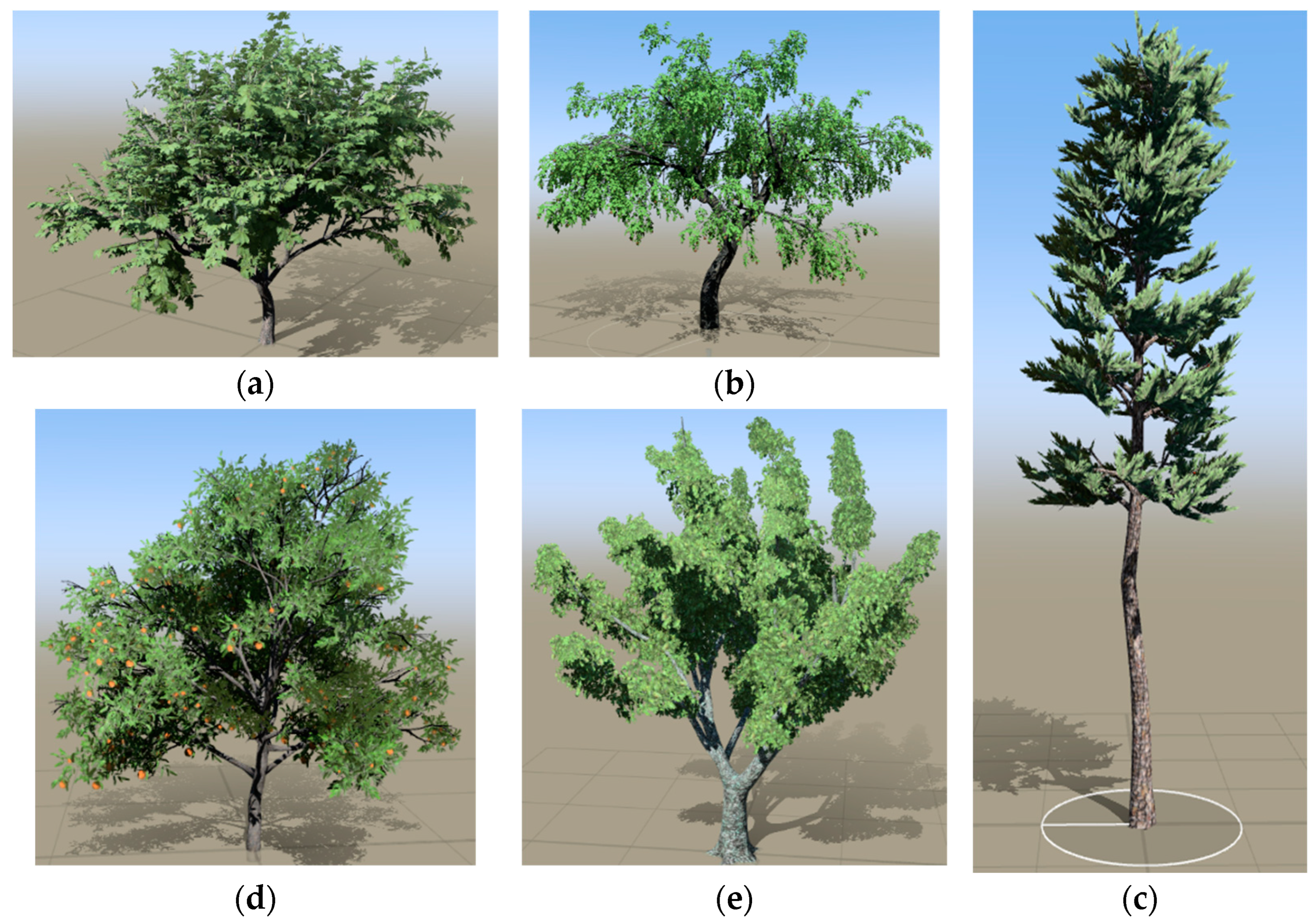
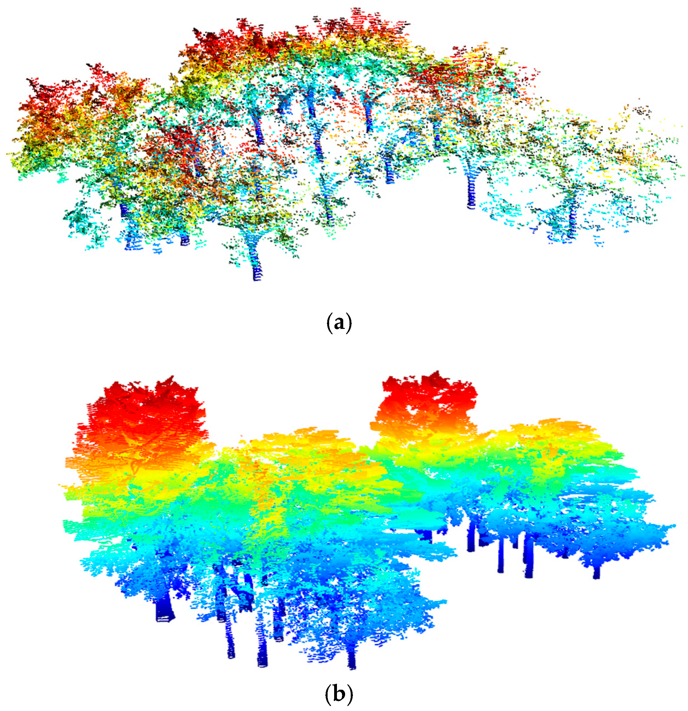
2.1.2. Point Cloud Data Simulation

The forest point cloud data with vertical structure used in this paper are modeled by SpeedTree V8.4.0 and simulated by Helios++ V1.3.0 software [37]. Helios++ is an open-source tool, which allows users to simulate various laser scanning platforms on a virtual scene composed of grid models. In this study, the setting and specifications of RieglVZ-400 (0.3 mrad beam divergence angle, 0.05 angle resolution) are simulated, which is a scanner commonly used in forestry research. Simulated scanning from 8 locations, with 4 in the periphery and 4 in the corner. The point clouds from these multiple scans were assembled into a unified dataset using a fixed global coordinate system, eliminating the need for additional registration. Overlapping points were managed through proximity-based filtering, and ground points were removed using a slope-based filtering approach. This multi-view scanning methodology closely mimics real-world LiDAR surveys, enhancing the accuracy of trunk extraction and vertical structure analysis. The distribution of specific trees and stations is shown in Figure 1.

SpeedTree V8.4.0 is widely used in industry to model various tree species and forests in games or movies, and it has a strong simulation engine for real tree species models and physical simulation in the real world [38]. Based on this software, this study established a variety of tree models to meet the complex tree species conditions in different forest environments (Figure 2).

2.2. Methods

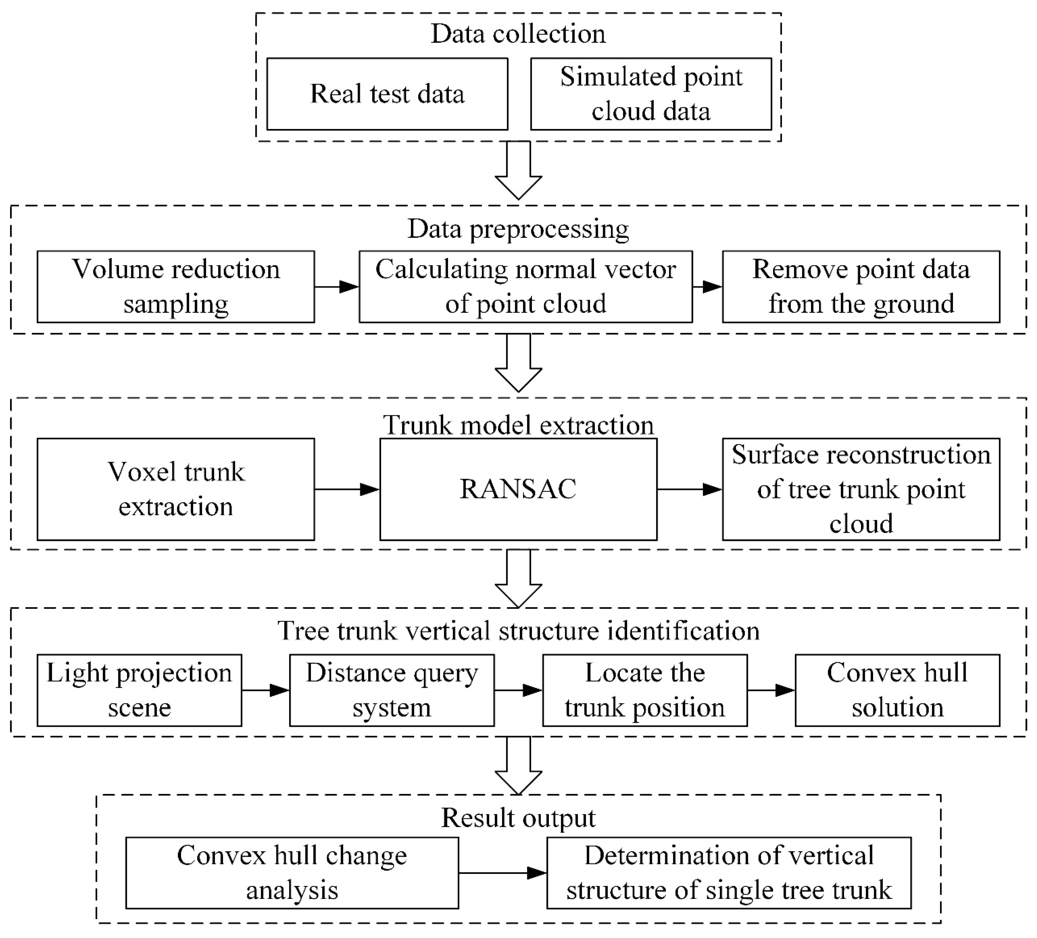
2.2.1. Method Flowchart

The methodological flowchart of this research is shown in Figure 3. After data preprocessing, this method uses the Layer Stacking model [39] to transform the structural analysis of trees and crowns into the study of single tree trunks, leveraging the positive correlation between trunk height, crown, and overall tree height. Based on variations in trunk height, a voxel-based shape recognition algorithm is designed to extract the trunk structure from tree point clouds. Then, the RANSAC algorithm is applied to address discontinuities in the vertical trunk structure generated by the above method. The Alpha Shapes algorithm is then utilized to reconstruct the surface of the tree point cloud. To further refine the analysis, tree trunk locating points are identified as specific spatial markers along the trunk at various heights. These points are determined by simulating a light projection scene, in which virtual uniform light source points are introduced into the point cloud scene to establish a distance query system. This system enables precise determination of the tree trunk coordinates at different vertical heights, effectively delineating the spatial and structural characteristics of the trunk. Finally, the convex hull of the lowest tree trunk locating points is computed using the Graham scan algorithm [40], and the vertical structure consistency of individual tree trunks is evaluated based on variations in internal positioning points at different heights.

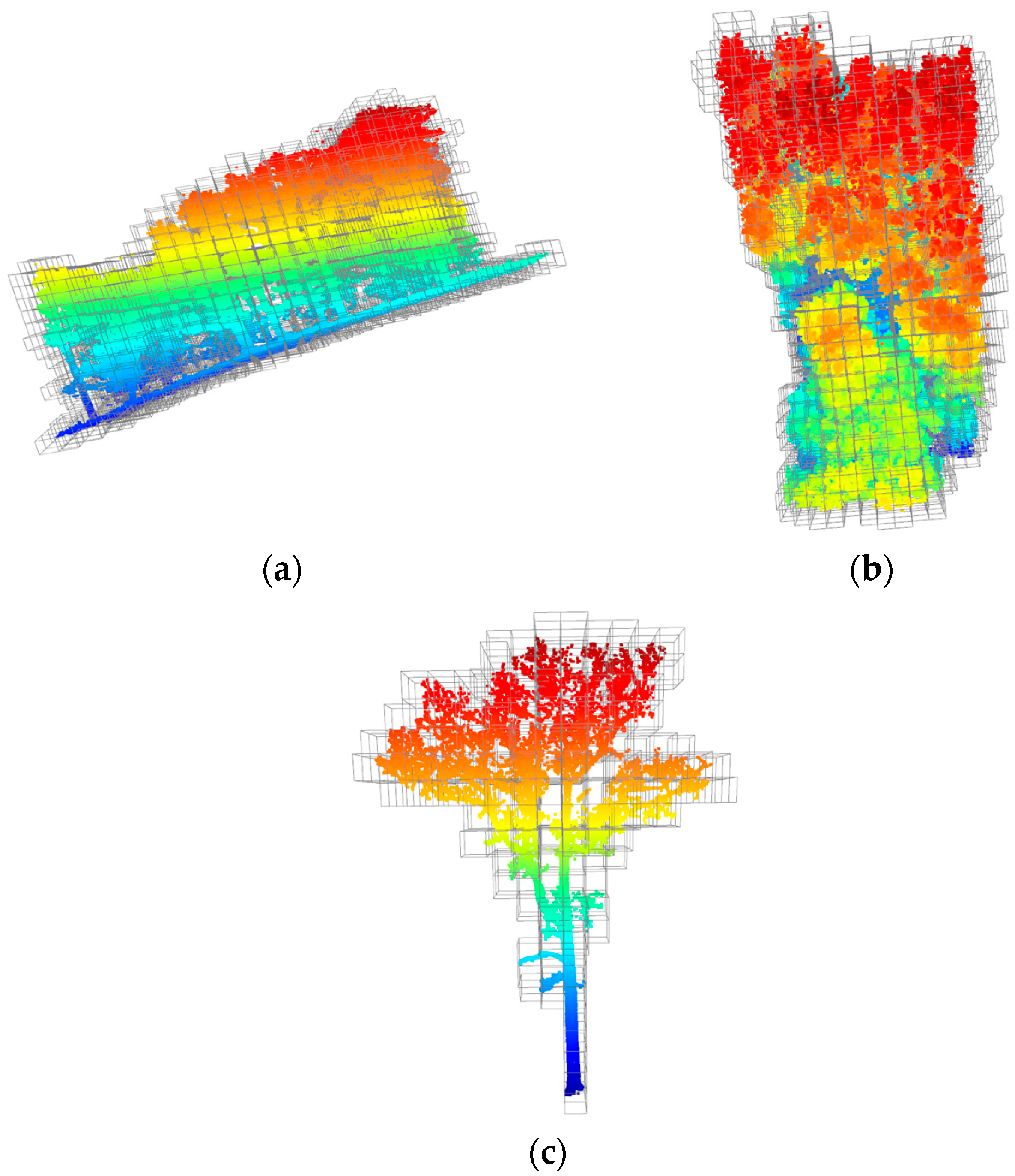
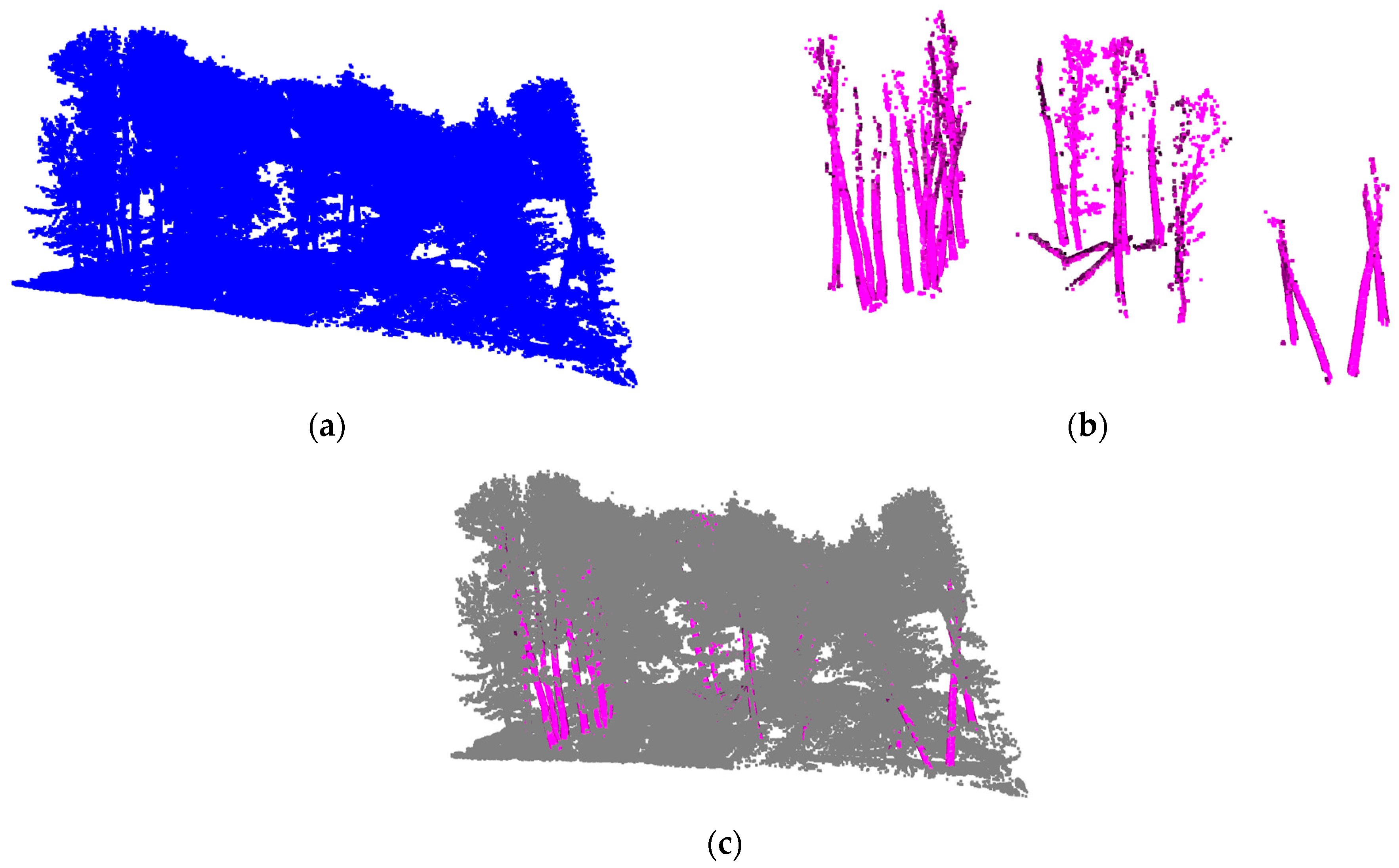
2.2.2. A Voxelized Trunk Extraction Algorithm

In a complex forest ecosystem, the trunks of trees usually present a linear feature, and the branches of trees, the ground, and the weeds on the ground all show planar or spherical features. Therefore, this study employs voxel-based shape recognition algorithms, including voxelization and voxel-based dimension analysis. Finally, a set of linear point clouds is generated and used as the input for the subsequent modules.

(1)

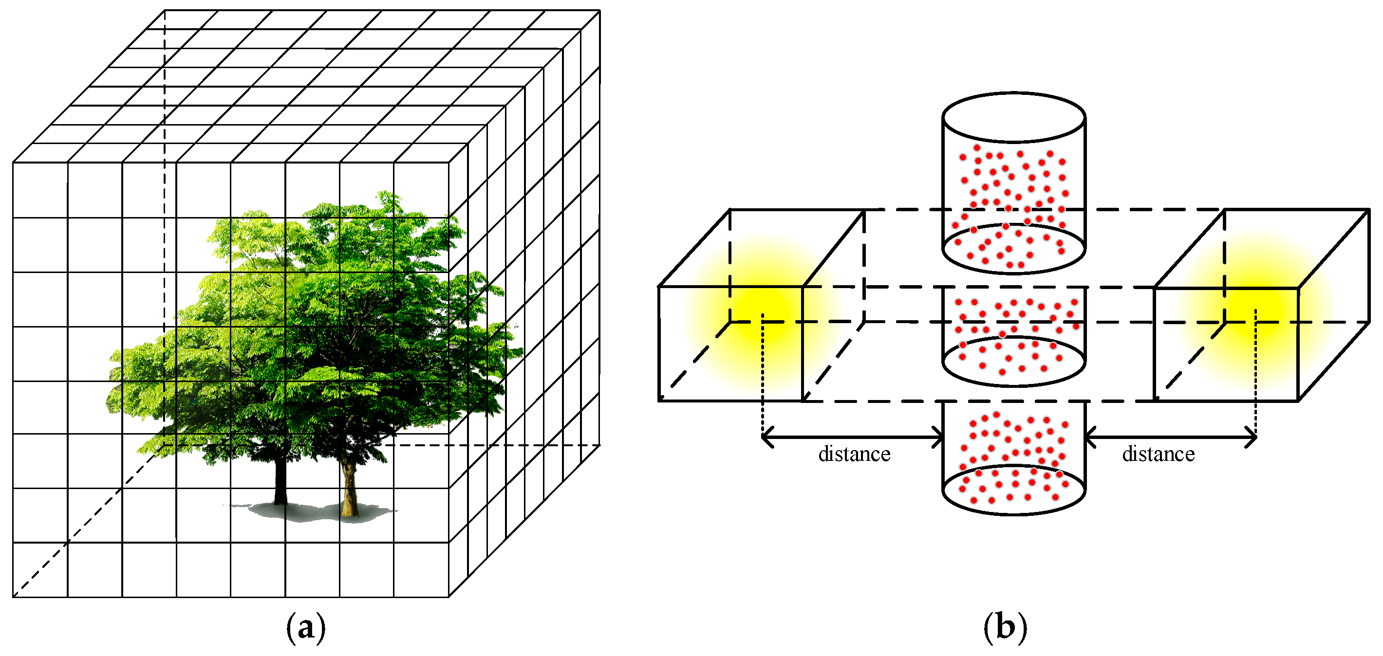
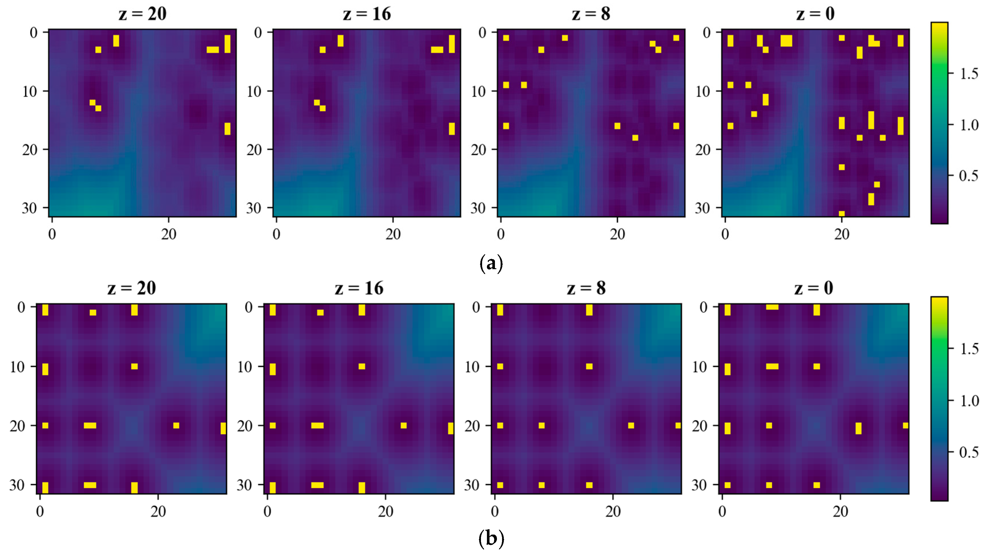
Voxelization: LiDAR point cloud data contains a large number of point elements used to describe the three-dimensional features in the scene. To reduce the amount of data processing, 3D voxels are constructed based on the XYZ coordinate system, and the point cloud data are divided into regular 3D grids, where each voxel is a cube with a side length of l. Any voxel can be indexed by the row (i), column (j), and layer (k), and equally divided in the XYZ coordinate system.

According to the minimum values ($x_{\mathrm{m}\mathrm{i}\mathrm{n}}, y_{\mathrm{m}\mathrm{i}\mathrm{n}}, z_{\mathrm{m}\mathrm{i}\mathrm{n}}$) in the coordinate system and the side length (l) of voxels, the voxel index ($i, j, k$), to which each point belongs, can be calculated by using Equations (1)–(3):

$$i=(x-x_{\min })/l,$$

(1)

$$j=(y-y_{\min })/l,$$

(2)

$$k=(z-z_{\mathrm{m}\mathrm{i}\mathrm{n}})/l.$$

(3)

(2)

Voxel-based dimension analysis: After voxelizing the point cloud data, this paper uses principal component analysis (PCA) as the main method to analyze the voxel dimension. PCA is a widely accepted dimensional analysis method, and it is widely used to infer geometric types of point cloud data. The common inference types are the following three types of shapes: linear, planar, and spherical [41].

The voxel dimension analysis mainly analyzes the local shape of the point cloud inside the voxel. Because the size of a voxel directly determines the number of points it contains, this may affect the effectiveness of dimensional analysis. Therefore, to better describe the geometric structure around point $p$, we denote the geometric center $p$ of the target voxel as the spherical center, set the neighborhood with the predefined value R as the radius, and search all the points in its interior and adjacent voxels as the point set to describe its local geometric structure. The covariance matrix $C_p$ of the above point set can be solved by Equation (4).

$$C_p={\displaystyle \frac{1}{N}}{\sum }_{p_i\subseteq N}(p_i-\overline{p})(p_i-\overline{p}{)}^T,$$

(4)

where $N$ is the number of points in the neighborhood, $p_i$ is the coordinates of the individual points (x, y, z) within the neighborhood, $\overline{p}={\displaystyle \frac{1}{N}}\sum _{p_i\subseteq N}{p}_i$.

${\lambda }_1>{\lambda }_2>{\lambda }_3>0$ is used as the normalized eigenvalue of the covariance matrix $C_p$. For the two special cases of ${\lambda }_i={\lambda }_j (i, j=\mathrm{1,\; 2}, 3, i \ne j)$ and ${\lambda }_i=0 (i=\mathrm{1,\; 2}, 3)$, we choose to reduce the probability of this case by increasing the search radius. Here, we use indicators $a_{1\mathrm{d}}, a_{2\mathrm{d}}, a_{3\mathrm{d}}$ to determine whether the local geometric structure of the point cloud is linear, planar, or spherical. $a_{1\mathrm{d}}, a_{2\mathrm{d}}, a_{3\mathrm{d}}$ can be calculated as:

$$a_{1\mathrm{d}}={\displaystyle \frac{\sqrt{{\lambda }_1}-\sqrt{{\lambda }_2}}{\sqrt{{\lambda }_1}}},$$

(5)

$$a_{2\mathrm{d}}={\displaystyle \frac{\sqrt{{\lambda }_2}-\sqrt{{\lambda }_3}}{\sqrt{{\lambda }_1}}},$$

(6)

$$a_{3\mathrm{d}}={\displaystyle \frac{\sqrt{{\lambda }_3}}{\sqrt{{\lambda }_1}}}.$$

(7)

The predefined radius R will affect the results of dimensional analysis. If the predefined radius R is too small, the geometric structure of the point may be estimated incorrectly, while when the predefined radius R is too large, the recognition may be affected by noise. Therefore, the entropy function is used to determine the predefined radius R of each voxel. The entropy function can be expressed as:

$$R\in \left\{{\mathrm{R}}_{\mathrm{m}\mathrm{i}\mathrm{n}}+k{\mathrm{R}}_{\mathrm{s}\mathrm{t}\mathrm{e}\mathrm{p}}∣k\in {\mathrm{N}}_0,{\mathrm{R}}_{\mathrm{m}\mathrm{i}\mathrm{n}}+k{\mathrm{R}}_{\mathrm{s}\mathrm{t}\mathrm{e}\mathrm{p}}\le {\mathrm{R}}_{\mathrm{m}\mathrm{a}\mathrm{x}}\right\},$$

(8)

$$E_f\left(V_p^R\right)=-a_{1\mathrm{d}}\ln a_{1\mathrm{d}}-a_{2\mathrm{d}}\ln a_{2\mathrm{d}}-a_{3\mathrm{d}}\ln a_{3\mathrm{d}},$$

(9)

where ${\mathrm{R}}_{\mathrm{m}\mathrm{i}\mathrm{n}}$ and ${\mathrm{R}}_{\mathrm{m}\mathrm{a}\mathrm{x}}$ are defined as the minimum search radius and the maximum search radius, respectively, and ${\mathrm{R}}_{\mathrm{s}\mathrm{t}\mathrm{e}\mathrm{p}}$ is the incremental iteration step, ${\mathrm{N}}_0$ is a non−negative integer (including 0). The minimum entropy value $E_f\left(V_p^R\right)$ is found in the range of ${\mathrm{R}}_{\mathrm{m}\mathrm{i}\mathrm{n}}$ and ${\mathrm{R}}_{\mathrm{m}\mathrm{a}\mathrm{x}}$, and the corresponding radius R, the corresponding eigenvalues ${\lambda }_1,{\lambda }_2,{\lambda }_{3,}$ and the corresponding eigenvectors $v_1,v_2,v_3$ are recorded. The judgment conditions of $a_{1\mathrm{d}}, a_{2\mathrm{d}}, a_{3\mathrm{d}}$ are shown in

Table 2. Local shape judgment conditions.

Local Shape	Condition	Direction
Line	$a_{1\mathrm{d}}>a_{2\mathrm{d}}$$\mathrm{and} a_{1\mathrm{d}}>a_{3\mathrm{d}}$	$v_1$
Surface	$a_{2\mathrm{d}}>a_{1\mathrm{d}}$$\mathrm{and} a_{2\mathrm{d}}>a_{1\mathrm{d}}$	$v_3$
Sphere	$a_{3\mathrm{d}}>a_{1\mathrm{d}}$$\mathrm{and} a_{3\mathrm{d}}>a_{2\mathrm{d}}$	No direction

.

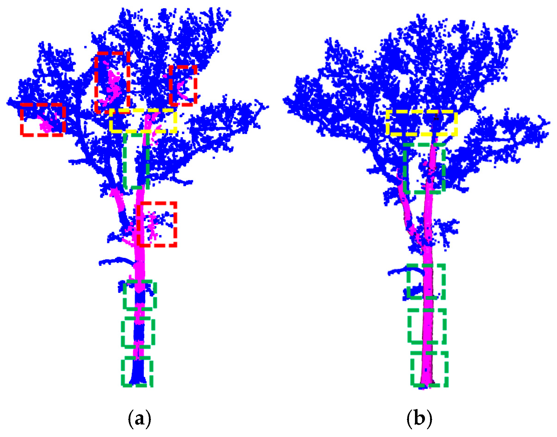
2.2.3. Extracting Discontinuous Vertical Structure and Robustness Test Based on RANSAC

RANSAC is a paradigm that randomly extracts the minimum set from point cloud data and constructs the corresponding shape prototype. A minimum set is a unique set of minimum points required for a given type of geometric archetype. The generated candidate shape will test all the points in the data (using the score function of the shape prototype) to determine how many points are approximated by the geometric prototype. After a given number of iterations, the shape prototype closest to the most points is extracted, the corresponding minimum set is deleted from the dataset, and then the remaining data will continue to be processed [42].

The algorithm needs to determine the type of sampled shape in advance, such as plane, surface, and cylinder, to obtain the parameter equation of the corresponding shape, and then facilitate the calculation of the shape fitted by the sampling points.

The algorithm is summarized as follows: the input of the algorithm is a set of point cloud data $\mathcal{P}=\left\{p_1,\dots ,p_N\right\}$ and its corresponding normal vectors $\{n_1,\dots ,n_N\}$, and the output is a set of disjoint point sets ${\mathcal{P}}_{{\psi }_1}\subset \mathcal{P},\dots ,{\mathcal{P}}_{{\psi }_n}\subset \mathcal{P}$ corresponding to the shape prototype $\Psi =\{{\psi }_1,\dots ,{\psi }_N\}$ and a set of segmented residual point sets $\mathrm{R}=\mathcal{P}\backslash \{{\mathcal{P}}_{{\psi }_1},\dots ,{\mathcal{P}}_{{\psi }_n}\}$. The intermediate variable is defined as the shape candidate $\mathcal{C}$, which is used to record the candidate of the shape calculated after sampling. Firstly, the algorithm initializes the shape prototype $\mathsf{\Psi }$ and the shape candidate $\mathcal{C}$ to an empty set. After that, the point cloud data are randomly sampled in multiple groups, and the corresponding parameter equations are calculated according to the sampling results and added into the shape candidates. Then, the candidate shape of the optimal score function is calculated from $\mathcal{C}$ by using the score function. This study uses the method of Schnabel et al. [42] which contains two special parameters: (1) the maximum distance $\epsilon$ between the sampling point and the shape itself, and (2) the normal vector of the point and the deviation angle $\alpha$ of the shape. The pseudo-code description of the algorithm is shown in Algorithm 1.

Algorithm 1 Extract the shapes in the point cloud $\mathcal{P}$

$\Psi =\mathrm{\varnothing }\left\{\mathrm{S}\mathrm{h}\mathrm{a}\mathrm{p}\mathrm{e} \mathrm{a}\mathrm{f}\mathrm{t}\mathrm{e}\mathrm{r} \mathrm{e}\mathrm{x}\mathrm{t}\mathrm{r}\mathrm{a}\mathrm{c}\mathrm{t}\mathrm{i}\mathrm{o}\mathrm{n}\right\}$ $\mathcal{C}=\mathrm{\varnothing }\{\mathrm{C}\mathrm{a}\mathrm{n}\mathrm{d}\mathrm{i}\mathrm{d}\mathrm{a}\mathrm{t}\mathrm{e} \mathrm{s}\mathrm{h}\mathrm{a}\mathrm{p}\mathrm{e}\}$ do $\mathcal{C}\leftarrow \mathcal{C}\cup \mathrm{n}\mathrm{e}\mathrm{w}\mathrm{C}\mathrm{a}\mathrm{n}\mathrm{d}\mathrm{i}\mathrm{d}\mathrm{a}\mathrm{t}\mathrm{e}\mathrm{s}(\mathrm{C}\mathrm{o}\mathrm{n}\mathrm{s}\mathrm{t}\mathrm{r}\mathrm{u}\mathrm{c}\mathrm{t} \mathrm{a} \mathrm{n}\mathrm{e}\mathrm{w} \mathrm{c}\mathrm{a}\mathrm{n}\mathrm{d}\mathrm{i}\mathrm{d}\mathrm{a}\mathrm{t}\mathrm{e})$ $m\leftarrow \mathrm{b}\mathrm{e}\mathrm{s}\mathrm{t}\mathrm{C}\mathrm{a}\mathrm{n}\mathrm{d}\mathrm{i}\mathrm{d}\mathrm{a}\mathrm{t}\mathrm{e}\mathrm{s}\left(\mathcal{C}\right)\{\mathrm{S}\mathrm{e}\mathrm{l}\mathrm{e}\mathrm{c}\mathrm{t} \mathrm{t}\mathrm{h}\mathrm{e} \mathrm{c}\mathrm{a}\mathrm{n}\mathrm{d}\mathrm{i}\mathrm{d}\mathrm{a}\mathrm{t}\mathrm{e} \mathrm{p}\mathrm{o}\mathrm{i}\mathrm{n}\mathrm{t}$ $\mathrm{o}\mathrm{f} \mathrm{t}\mathrm{h}\mathrm{e} \mathrm{o}\mathrm{p}\mathrm{t}\mathrm{i}\mathrm{m}\mathrm{a}\mathrm{l} \mathrm{s}\mathrm{c}\mathrm{o}\mathrm{r}\mathrm{e} \mathrm{f}\mathrm{u}\mathrm{n}\mathrm{c}\mathrm{t}\mathrm{i}\mathrm{o}\mathrm{n}\}$

if  $P\left(\left|m\right|,\left|\mathcal{C}\right|\right)>p_t$ then $\mathcal{P}\leftarrow \mathcal{P}\backslash {\mathcal{P}}_m\{\mathrm{D}\mathrm{e}\mathrm{l}\mathrm{e}\mathrm{t}\mathrm{e} \mathrm{p}\mathrm{o}\mathrm{i}\mathrm{n}\mathrm{t}\}$

$\Psi \leftarrow \Psi \cup \mathrm{m}$ $\mathcal{C}\leftarrow \mathcal{C}\backslash {\mathcal{C}}_m\{\mathrm{D}\mathrm{e}\mathrm{l}\mathrm{e}\mathrm{t}\mathrm{e} \mathrm{i}\mathrm{n}\mathrm{v}\mathrm{a}\mathrm{l}\mathrm{i}\mathrm{d} \mathrm{c}\mathrm{a}\mathrm{n}\mathrm{d}\mathrm{i}\mathrm{d}\mathrm{a}\mathrm{t}\mathrm{e}\mathrm{s}\}$ end if until  $P\left(\tau ,\left|\mathcal{C}\right|\right)>p_t$ return  $\Psi$

The RANSAC method used in this experiment is the RANSAC cylinder recognition algorithm provided by the CloudCompare plug-in. In this algorithm, before sampling, the octree index of the whole point cloud is established, and a new candidate, $p_1$, is selected by global sampling. Then, any node $\mathcal{C}$ in the octree node containing $p_1$ is selected, and the remaining k-1 samples will be sampled in the space contained by $\mathcal{C}$ [42].

The algorithm uses three different evaluation angles for the evaluation of candidate prototypes: (a) The number of points falling into the neighborhood $\epsilon$ of candidate prototypes is calculated as the support degree of candidate prototypes. (b) In order to ensure that the large rank of the points falling into the neighborhood $\epsilon$ conforms to the curvature of the given prototype, the algorithm only considers the normal vector of the points and the points whose deviation of the normal vector projected on the prototype is less than $\alpha$. (c) The algorithm introduces the concept of connected components in two-dimensional images and only considers the largest connected components that make up the prototype. The formal expression of the above conditions is shown in Equations (10) and (11) [42].

$${\widehat{\mathcal{P}}}_{\psi }=\left\{p|p\in \mathcal{P}\wedge d\left(\psi ,p\right)<\epsilon \wedge \arccos \left(\left|n\left(p\right)·n\left(\psi ,p\right)\right|\right\}<\alpha \right\},$$

(10)

$${\mathcal{P}}_{\psi }=\mathrm{m}\mathrm{a}\mathrm{x}\mathrm{c}\mathrm{o}\mathrm{m}\mathrm{p}\mathrm{o}\mathrm{n}\mathrm{e}\mathrm{n}\mathrm{t}\left(\psi ,{\widehat{\mathcal{P}}}_{\psi }\right),$$

(11)

where ${\widehat{\mathcal{P}}}_{\psi }$ is the estimated shape prototype, ${\mathcal{P}}_{\psi }$ is the actual reserved shape prototype, $n\left(p\right)$ is the normal vector of point p, and $n\left(\psi ,p\right)$ is the normal vector of point p projected on the candidate $\psi$ graph.

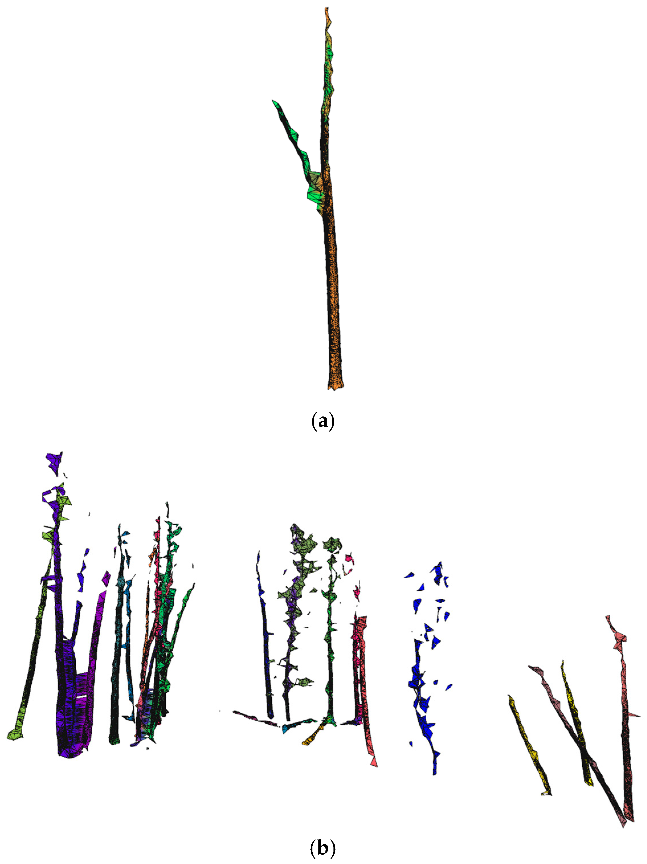
2.2.4. Trunk Surface Reconstruction

Because the subsequent light projection scene requires a continuous and complete trunk surface, the Alpha Shapes algorithm is employed solely for surface reconstruction. The construction of 3D Alpha Shapes can be visualized as shaping the convex hull of the original point set using an empty sphere with a user-specified radius alpha [43,44]. The optimal alpha value is determined through systematic experiments to ensure the reconstructed trunk surfaces are structurally consistent and well-formed. To ensure an objective evaluation of alpha selection, we compare our reconstruction results against manually labeled ground truth tree trunk data from the 3D forest dataset, allowing us to compute relevant performance metrics. Since Alpha Shapes is primarily used for reconstructing a smooth and continuous trunk surface rather than for trunk extraction, we evaluate its performance using the Trunk Surface Continuity Score (TSC) and Completeness Ratio (CR) to ensure the reconstructed surface maintains structural integrity and accuracy. The formula is as follows:

$$TSC=1-{\displaystyle \frac{{\sum }_{i=1}^N\left|d_i-\overline{d}\right|}{N\overline{d}}},$$

(12)

$$CR={\displaystyle \frac{N_o}{N_t}},$$

(13)

where $d_i$ is local trunk diameter at point $i$, $\overline{d}$ is the expected trunk diameter from the 3D forest dataset (ground truth), $N$ is total number of sampled points along the trunk, $N_o$ is the number of points in the reconstructed model that overlap with the ground truth point cloud, and $N_t$ is the total number of points in the ground truth model.

2.2.5. Locating the Trunk Position in the Light Projection Scene

The light projection scene is introduced to locate the position of the trunk. The light projection scene is a group of regularly distributed light source arrays horizontally projected on a three-dimensional surface, and the projection direction of the light source horizontally points to the vertical central axis of the scene. When the light is projected onto the 3D surface, the light source point will return to the distance projected by the light source point onto the 3D surface. The projection principle of the light source array and the query principle of the distance query system are shown in Figure 4.

The light source array and distance query system are implemented using the Open3D open-source 3D data processing library to analyze the surface structure of tree trunks [45]. The system returns a tensor T ($n\times m\times k$), where n, m, and k correspond to evenly spaced grid divisions along the coordinate axes, representing the distance from each projected light source to the nearest point on the tree trunk surface. By slicing T along the Z-axis, we obtain 2D distance maps at different heights. In regions with tree trunks, the distance values decrease as the slicing height approaches the trunk, due to the proximity of the trunk surface. This variation in distance values enables accurate trunk localization and provides insights into vertical structural changes.

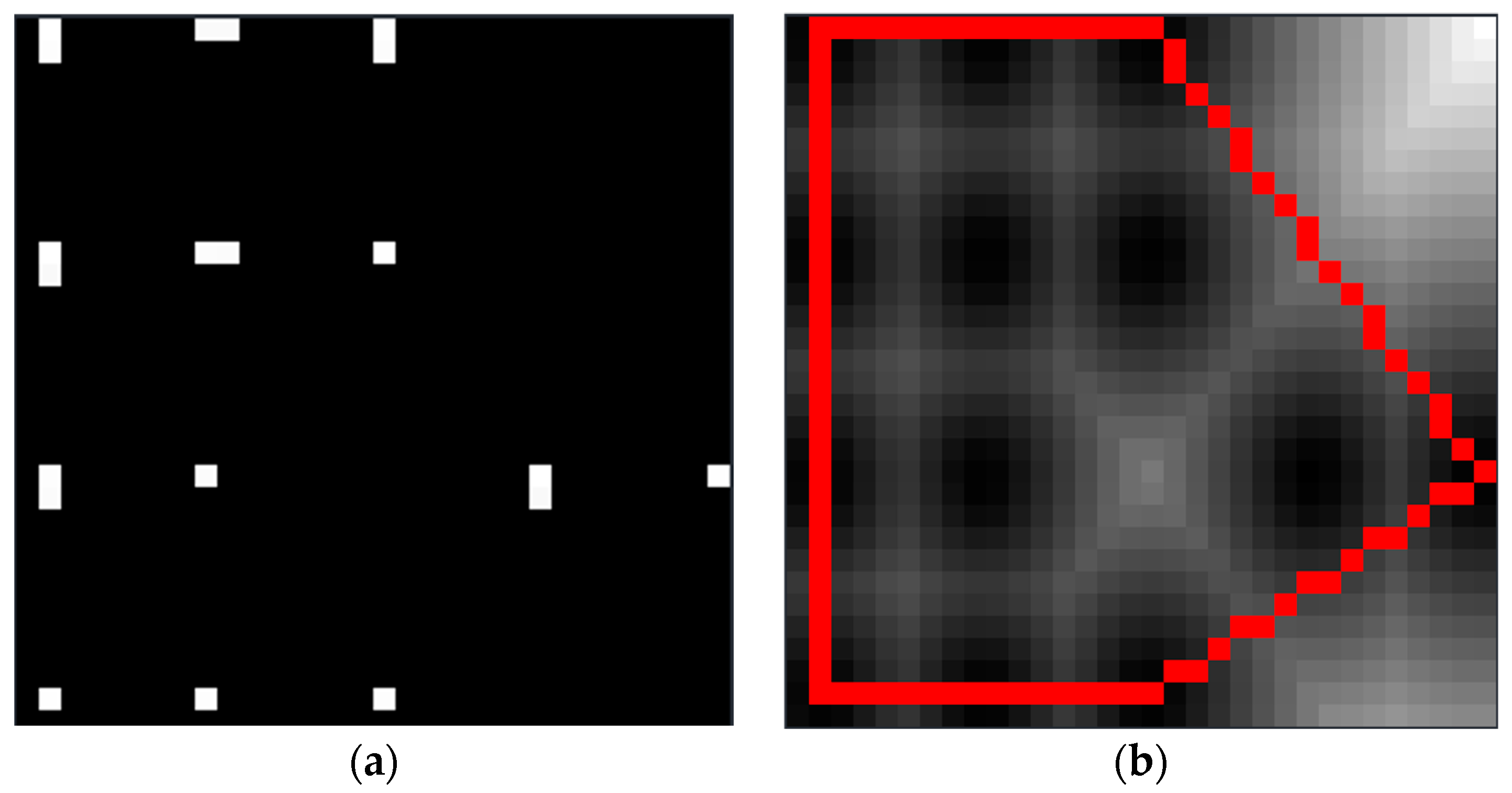
2.2.6. Algorithm for Solving Trunk Positioning Point Convex Hull and Determination of Vertical Structure of Single Tree Trunk

By comparing slice images of the vertical trunk height distribution of a single tree, it is found that the difference in the number of trunks extracted by the sectional data with the same vertical structural characteristics of trunks at different Z values is smaller. Also, the shape is fixed compared with the sectional data about different vertical structural characteristics of trunks. According to the above characteristics, we introduce a convex hull solution algorithm to determine the convex hull shape of tree trunk locating points at different Z-value slices, and we calculate the change difference in trunk locating points in the current convex hull. According to the change in the number of locating points in the convex hull, we can approximately determine whether the trees in the current convex hull have vertical stratification structure. Therefore, this algorithm consists of two parts: (1) The solution and editing of the convex hull when Z = 0. (2) According to the change in the number of trunk locating points in the convex hull, the vertical structural characteristics of single tree trunk are determined.

The Graham scanning method [40] is used in the convex hull solving algorithm in this paper. The input of the Graham scanning method is trunk positioning point Q, where $\left|Q\right|\ge 3$ is required. The Graham scanning method solves the convex hull problem by setting a stack S about candidate points. Each point in the set Q is pushed into the stack S once, and the point for the non−convex hull vertex is finally popped out of the stack. When the algorithm is terminated, the stack S only contains the vertices in the convex hull, and they appear on the boundary of the convex hull from the bottom to the top in an anticlockwise order.

3. Results

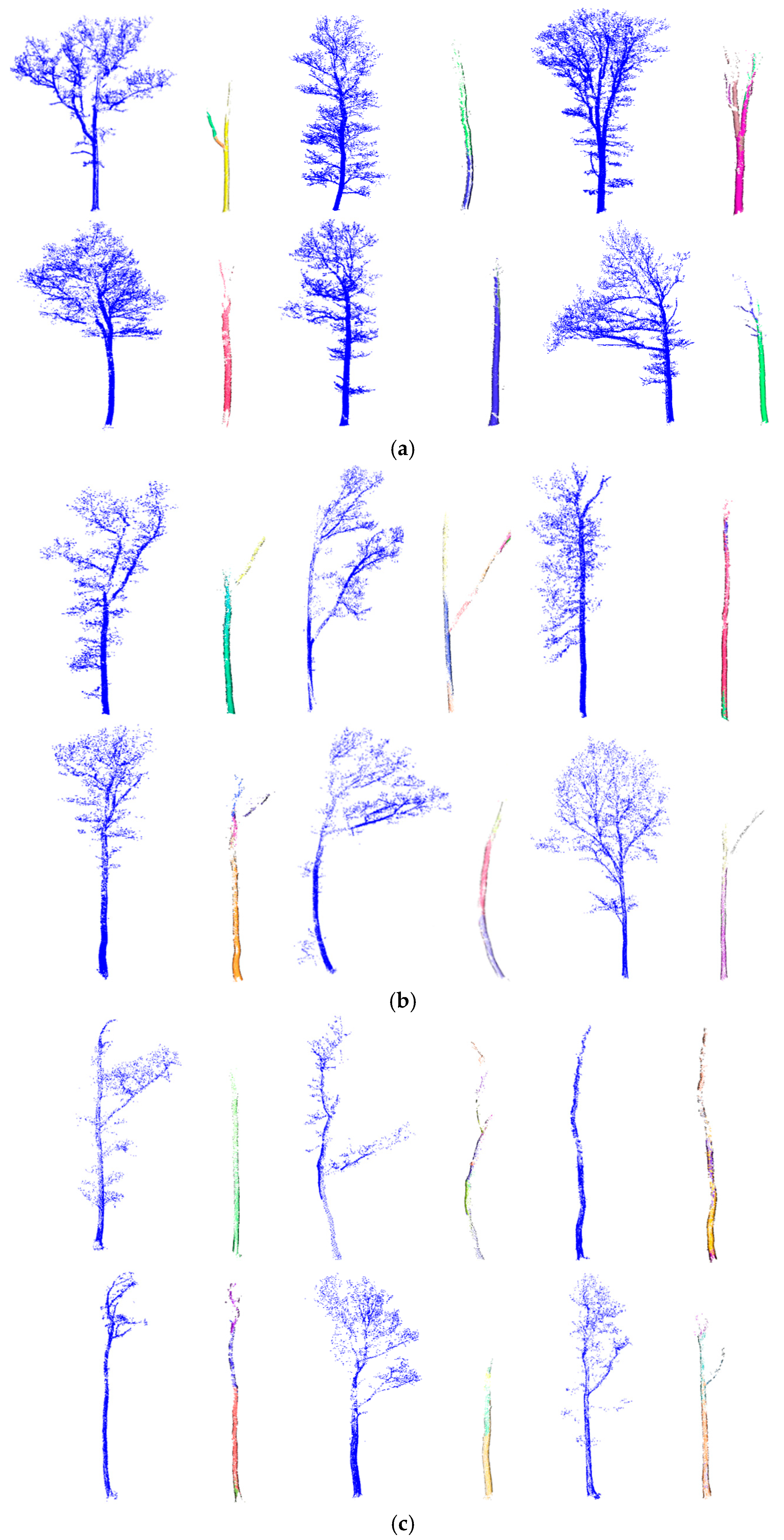
3.1. Single Trees

Based on the above method, a large amount of point cloud data can be divided into different voxels. The results of point cloud voxelization in 3D Forest test data are shown in Figure 5a,b below, and the voxels of a single tree are shown in Figure 5c.

Based on the RANSAC algorithm mentioned above, this study divides the point clouds with linear characteristics segmented by the voxel-based trunk extraction algorithm into different minimum sets according to the boundary of voxels, calculates the candidate cylindrical shapes, and then evaluates them with the score function. The point clouds in the dotted red box in Figure 6a are screened out and the connectivity of the point clouds is considered to complete the unconnected areas in the trunk (in the dotted green box in Figure 6a). Due to the scanning of LiDAR, the trunk point cloud cannot show the complete circle characteristics of the cylinder completely, so it cannot pass the score function (in the dotted yellow box in Figure 6).

The above method is applied to 3D Forest data, and the extraction results are shown in Figure 7.

The light projection scene is introduced to better query the number of trunks at different heights, so the result of surface reconstruction does not need to consider the gap between the generated surface data and the real data. However, the selection of surface reconstruction parameter setting should pay attention to the continuity of the surface of a single tree, while ensuring the independence of trunk points of different trees. Based on prior research, we defined an alpha range from 0.10 to 0.50 with a step size of 0.05 and systematically tested each alpha on LiDAR point clouds from different forest environments.

Table 3. Alpha parameter selection and performance evaluation.

Metrics	Alpha
	0.1	0.15	0.2	0.25	0.3	0.35	0.4	0.45	0.5
TSC	0.74	0.76	0.79	0.82	0.84	0.86	0.84	0.81	0.78
CR	0.75	0.78	0.81	0.85	0.88	0.91	0.88	0.84	0.80

provides a summary of our experimental results, while the optimal reconstruction outcomes are illustrated in Figure 8.

The results indicated that alpha = 0.35 provided the optimal balance, yielding the highest TSC and CR. Lower alpha values (0.10–0.25) led to a decrease in SC, causing surface discontinuities and fragmentation in the reconstructed trunks. In contrast, higher alpha values (0.40–0.50) reduced CR, leading to excessive surface smoothing and loss of fine structural details, which impacted the completeness of the reconstruction.

3.2. RANSAC Robustness Test

Based on the above RANSAC algorithm, this study selected different tree point clouds in the same forest for experiments and discussed the accuracy of the RANSAC algorithm in tree trunk recognition under different tree shapes and different parameter settings. The parameter settings of each group are shown in

Table 4. Parameter Setting and Identification Results.

Group	$|\mathcal{P}$|	$\mathit{\alpha }$	$\mathit{\epsilon }$	$\mathit{C}$	${\mathit{p}}_{\mathit{t}}$	$\left|\mathit{\psi }\right|$
0	10 k~39 k	${\displaystyle \frac{5}{36}}\pi$	0.08~0.92	0.161~0.252	0.01	1~3
1	5 k~10 k	${\displaystyle \frac{5}{36}}\pi$	0.107	0.214	0.01	1~4
2	0~5 k	${\displaystyle \frac{5}{36}}\pi$	0.115	0.210	0.01	2~6

.

Partial results of the above experiments are shown in Figure 9.

According to the experiments of the above three groups of different point cloud densities, the RANSAC algorithm can complete the identification of trunk point clouds by setting the minimum sampling scale between 5 and 10 points, depending on the point cloud density. No significant modification of other parameters, such as the inlier threshold or maximum iteration count, was required across different experiments. From the recognition effect point of view, the algorithm performs better for the lower part of the trunk, where there are fewer branches. However, the accuracy of the algorithm drops significantly for the upper part, where branches diverge, especially in areas with dense leaf coverage and occlusions. Despite varying preprocessing requirements across tree species, the experimental results show that the recognition results generally meet the identification requirements for trunk point clouds.

3.3. Trunk Locating

We combined the modular species established in Section 2.1.2 with the tree layout shown in Figure 2, thus the simulated scanning data point cloud can be obtained as shown in Figure 10 (this point cloud is the point cloud data after filtering the ground points).

In the forest area with significant vertical stratification structure, when the Z-axis of T is sliced at different heights, the obtained two-dimensional data should have obvious changes compared with those without significant vertical stratification structure. Figure 11 shows the comparison results of different height slices of forest areas with significant vertical stratification and those without significant vertical stratification, respectively. The larger the value in the slice, the fewer trunks in the current position in the height slice, and the larger the coverage area without trunks.

Through the analysis of the above results in Figure 11, it can be seen that the query results generated in forest areas with inconsistent vertical structure of individual tree trunks from Z = 0 to Z = 32 are obviously different. The tree trunks are obviously reduced, while the query results generated in forest areas with almost the same vertical structure of individual tree trunks from Z = 0 to Z = 32 are not obviously different, and the number of tree trunks is mainly unchanged. According to the above experimental results, the closer the value in the slice is to the trunk, the smaller the value is or even 0. According to this rule, the points with data which is less than a specific threshold, $\tau$, can be set as singular values outside the threshold, which can be used to locate the positions of trunk points (Figure 12).

3.4. Vertical Structural Characteristics of Trunk

The convex hull for solving the trunk locating point based on the simulation data are shown in Figure 13.

Through the analysis of the change in the trunk locating point of the convex hull, experimental results show that when the proportion of the trunk locating point reduction in the convex hull exceeds the proportion of low trees in the total count, the forest area can be identified as having inconsistent vertical structure in single tree trunks. To further validate this relationship, we conducted a series of experiments in simulated forest environments, analyzing changes in trunk locating points at different height slices. We found that when the proportion of points within the convex hull decreased by more than 50%, it corresponded to significant structural changes in the tree trunk’s vertical profile, often reflected by abrupt reductions in trunk diameter or noticeable changes in cross-sectional shape. Through experiments across various forest regions, we repeatedly confirmed the effectiveness of this 50% threshold, ultimately establishing it as an empirical indicator for identifying vertical structure inconsistency in tree trunks.

4. Discussion

The main process of forest vertical structure division can be summarized as single tree extraction and tree morphology detection and segmentation from pre-processed forest LiDAR data, including stem detection, leaf area index calculation, and canopy detection. On the basis of the above data, the vertical structure of the whole forest is analyzed [22,24,25]. The advantage of this method lies in the detailed morphological calculation and analysis of the single tree level in the forest. When applied to subsequent forest-level analyses, such as vertical structure analysis, canopy cover estimation, and tree species classification, it provides high accuracy. However, when only analyzing the vertical structure of forest, this process will be cumbersome, consume more time and costs, and generate more miscellaneous data, because there is no need to calculate other aspects of forest investigation in the follow-up. Therefore, a calculation method that can ensure the accuracy of forest vertical structure judgment without calculating various morphological factors is urgently needed in forestry investigation.

In this paper, the tree trunk shape recognition and the RANSAC algorithms are used to achieve the voxel segmentation of forest trees. On this basis, the convex hull of the tree trunk point is solved by locating the trees in the light projection, so as to determine the vertical structure of forest trees. Our proposed method enhances trunk extraction and vertical structure analysis by overcoming the limitations of existing approaches. Compared to hierarchical segmentation methods that rely on canopy detection [25], our approach improves trunk connectivity through voxel-based segmentation and RANSAC refinement, making it more effective in dense forests. Unlike semantic segmentation techniques focused on leaf-wood classification [26], our method prioritizes structural continuity by integrating light projection and the Alpha Shapes surface reconstruction, ensuring higher accuracy in trunk detection. Additionally, it outperforms traditional point cloud segmentation methods by enhancing robustness to noise, reducing segmentation fragmentation, and minimizing manual parameter tuning, making it a scalable and efficient solution for large-scale forest datasets and 3D reconstruction applications.

5. Conclusions

This study aimed to develop a novel approach for estimating tree vertical structure and trunk characteristics using LiDAR data. The research introduced a voxelized trunk extraction algorithm, which is designed to accurately determine the location and vertical structure of single tree trunks in forest environments. The method involved several key steps: first, a voxel-based shape recognition algorithm was applied to extract the trunk structure from tree point clouds. The vertical structure connectivity problem of the tree trunks was then solved using the RANSAC method. The Alpha Shapes algorithm was selected for surface reconstruction of the tree point clouds. To locate the tree trunk coordinates at different heights, a light projection scene was introduced based on the tree surface model. The convex hull of the trunk base was then computed using the Graham scanning method. The results demonstrated that the proposed single tree extraction algorithm, coupled with the vertical structure recognition algorithm in the light projection scene, effectively delineated regions where vertical structure distribution of single tree trunks was inconsistent. These findings highlight the potential of the proposed methods for improving forest resource surveys and the analysis of forest vertical structure. Specifically, the findings are as follows:

(1)

Taking the linear shape solved by trunk recognition algorithm as the candidate shape of the RANSAC algorithm can effectively solve the connectivity problem of trunk point cloud in the vertical direction.

(2)

Introducing the light projection scene can extract and count the trunk position accurately.

(3)

In forest areas where the vertical structure of individual tree trunks differs in the light projection scene, the location points of the tree trunks show significant changes. Experimental data indicate that the rate of change exceeds 50%.

These findings suggest that the proposed approach has the potential to significantly improve forest resource surveys and tree vertical structure analysis. By improving the accuracy of tree trunk modeling and vertical structure identification, this will contribute to more precise forest inventory and provide valuable support for ecological monitoring and forest management efforts. However, there are some limitations to this study. Firstly, because the data used in this experiment are 3D Forest real test data and point cloud data simulated by simulation software, the forest types are relatively single, and the above conclusions do not necessarily meet the growth characteristics of all trees. In particular, the current experimental setup primarily involves single-species tree distributions, and the algorithm’s adaptability to mixed-species forests with varying trunk and canopy structures remains to be further explored. Secondly, there are still many inadequacies in the robustness and accuracy of algorithm segmentation, and many difficult problems have not been solved. For the forest scene in practical application, the structural characteristics of forest point cloud tree height still need to solve the problems of litter, shrubs and broken discontinuous terrain in the actual point cloud scanning area. In addition, the preprocessing stage of this method depends on many different algorithms, and its robustness and accuracy are still a problem worth discussing. Future improvements should focus on enhancing the algorithm’s robustness and accuracy by expanding the data diversity to include a wider range of forest types, adapting it to mixed-species forests with varying trunk morphologies and canopy structures, improving tree trunk segmentation through advanced methods such as deep learning, and addressing challenges posed by obstacles like litter, shrubs, and irregular terrain. Additionally, optimizing the integration of various preprocessing algorithms and reducing their dependencies will help improve efficiency and reliability. Further validation in real-world forests with diverse ecosystems is necessary to ensure that the method can accurately capture tree growth characteristics across different species and environmental conditions.

References

- Ding, R. Importance of Forest Resources Investigation and Optimization Measures. World Trop. Agric. Inf. 2022, 4, 60–61. [Google Scholar]
- Xie, X.; Su, H.; Yang, Y.; Li, C.; Lu, F.; Luo, W.; Xu, Z. Estimation of stand parameters of eucalyptus plantation in Guangxi based on terrestrial laser scanner. For. Resour. Manag. 2022, 2, 100–108. [Google Scholar]
- Zhao, L. Application and prospect of airborne laser scanner in obtaining forest resource parameters. For. Sci. Technol. Inf. 2022, 54, 71–73. [Google Scholar]
- Dilixiati, B.; Halike, Y.; Yusufu, A.; Wei, J. Estimation of Populus euphratica leaf area index in the lower reaches of Tarim River by terrestrial laser scanner data. J. Northeast. For. Univ. 2020, 48, 46–50. [Google Scholar]
- Ross, N.; Jimenez, J.; Schnell, C.E.; Hartshorn, G.S.; Gregoire, T.G.; Oderwald, R. Canopy height models and airborne lasers to estimate forest biomass: Two problems. Int. J. Remote Sens. 2000, 21, 2153–2162. [Google Scholar]
- Luo, H.; Shu, Q.; Xi, L.; Huang, J.; Liu, Y.; Yang, Q. Research progress of estimating forest biomass by lidar. Green Technol. 2022, 24, 23–28. [Google Scholar]
- Chen, Q.; Qi, C. Lidar remote sensing of vegetation biomass. Remote Sens. Nat. Resour. 2013, 399, 399–420. [Google Scholar]
- Clark, M.L.; Roberts, D.A.; Ewel, J.J.; Clark, D.B. Estimation of tropical rain forest aboveground biomass with small-footprint lidar and hyperspectral sensors. Remote Sens. Environ. 2011, 115, 2931–2942. [Google Scholar]
- Wulder, M.A.; White, J.C.; Nelson, R.F.; Næsset, E.; Ørka, H.O.; Coops, N.C.; Gobakken, T. Lidar sampling for large-area forest characterization: A review. Remote Sens. Environ. 2012, 121, 196–209. [Google Scholar]
- Dong, P.; Chen, Q. LiDAR Remote Sensing and Applications; CRC Press: Boca Raton, FL, USA, 2017. [Google Scholar]
- Qi, Z.; Li, S.; Yue, W.; Liu, Q.; Li, Z. Natural forest gap identification based on drone laser scanner. J. Beijing For. Univ. 2022, 44, 44–53. [Google Scholar]
- Zhang, K. Identification of gaps in mangrove forests with airborne LIDAR. Remote Sens. Environ. 2008, 112, 2309–2325. [Google Scholar] [CrossRef]
- Zhu, B.; Jin, J.; Luo, H.; Long, F.; Li, C.; Yue, C. Inversion of average stand height byairborne laser scanner based on variable optimization. Jiangsu J. Agric. Sci. 2022, 38, 706–713. [Google Scholar]
- Wallace, A.; Nichol, C.; Woodhouse, I. Recovery of forest canopy parameters by inversion of multispectral LiDAR data. Remote Sens. 2012, 4, 509–531. [Google Scholar] [CrossRef]
- Moorthy, S.M.K.; Calders, K.; Vicari, M.B.; Verbeeck, H. Improved supervised learning-based approach for leaf and wood classification from LiDAR point clouds of forests. IEEE Trans. Geosci. Remote Sens. 2019, 58, 3057–3070. [Google Scholar] [CrossRef]
- Cao, L.; Coops, N.C.; Innes, J.L.; Dai, J.; Ruan, H.; She, G. Tree species classification in subtropical forests using small-footprint full-waveform LiDAR data. Int. J. Appl. Earth Obs. Geoinformation 2016, 49, 39–51. [Google Scholar] [CrossRef]
- Lou, Y.; Fan, Y.; Dai, Q.; Wang, Z.; Ku, W.; Zhao, M.; Yu, S. Relationship between the vertical structure of evergreen deciduous broad-leaved forest community and the overall species diversity of the community in Mount Tianmu. J. Ecol. 2021, 41, 8568–8577. [Google Scholar]
- Huang, W.; Pohjonen, V.; Johansson, S.; Nashanda, M.; Katigula, M.; Luukkanen, O. Species diversity, forest structure and species composition in Tanzanian tropical forests. For. Ecol. Manag. 2002, 173, 11–24. [Google Scholar] [CrossRef]
- Gui, X.; Lian, J.; Zhang, R.; Li, Y.; Shen, H.; Ni, Y.; Ye, W. Vertical structure and species diversity characteristics of subtropical evergreen broad-leaved forest community in Dinghushan. Biol. Divers. 2019, 27, 619–629. [Google Scholar]
- Jarron, L.R.; Coops, N.C.; MacKenzie, W.H.; Tompalski, P.; Dykstra, P. Detection of sub-canopy forest structure using airborne LiDAR. Remote Sens. Environ. 2020, 244, 111770. [Google Scholar] [CrossRef]
- de Almeida, D.R.A.; Zambrano, A.M.A.; Broadbent, E.N.; Wendt, A.L.; Foster, P.; Wilkinson, B.E.; Salk, C.; Papa, D.d.A.; Stark, S.C.; Valbuena, R.; et al. Detecting successional changes in tropical forest structure using GatorEye drone-borne lidar. Biotropica 2020, 52, 1155–1167. [Google Scholar] [CrossRef]
- Zhang, J.; Wang, J.; Liu, G. Vertical Structure Classification of a Forest Sample Plot Based on Point Cloud Data. J. Indian Soc. Remote Sens. 2020, 48, 1215–1222. [Google Scholar]
- Putman, E.B.; Popescu, S.C.; Eriksson, M.; Zhou, T.; Klockow, P.; Vogel, J.; Moore, G.W. Detecting and quantifying standing dead tree structural loss with reconstructed tree models using voxelized terrestrial lidar data. Remote Sens. Environ. 2018, 209, 52–65. [Google Scholar]
- Taheriazad, L.; Moghadas, H.; Sanchez-Azofeifa, A. Calculation of leaf area index in a Canadian boreal forest using adaptive voxelization and terrestrial LiDAR. Int. J. Appl. Earth Obs. Geoinf. 2019, 83, 101923. [Google Scholar]
- Zhong, L.; Cheng, L.; Xu, H.; Wu, Y.; Chen, Y.; Li, M. Segmentation of individual trees from TLS and MLS data. IEEE J. Sel. Top. Appl. Earth Obs. Remote Sens. 2016, 10, 774–787. [Google Scholar]
- Wang, D. Unsupervised semantic and instance segmentation of forest point clouds. ISPRS J. Photogramm. Remote Sens. 2020, 165, 86–97. [Google Scholar]
- Li, Z.; Wang, J.; Zhang, Z.; Jin, F.; Yang, J.; Sun, W.; Cao, Y. A Method Based on Improved iForest for Trunk Extraction and Denoising of Individual Street Trees. Remote Sens. 2022, 15, 115. [Google Scholar] [CrossRef]
- Neuville, R.; Bates, J.S.; Jonard, F. Estimating Forest Structure from UAV-Mounted LiDAR Point Cloud Using Machine Learning. Remote Sens. 2021, 13, 352. [Google Scholar] [CrossRef]
- Xu, S.; Sun, X.; Yun, J.; Wang, H. A New Clustering-Based Framework to the Stem Estimation and Growth Fitting of Street Trees From Mobile Laser Scanning Data. IEEE J. Sel. Top. Appl. Earth Obs. Remote Sens. 2020, 13, 3240–3250. [Google Scholar]
- Monnier, F.; Vallet, B.; Soheilian, B. Trees Detection From Laser Point Clouds Acquired in Dense Urban Areas by a Mobile Mapping System. ISPRS Ann. Photogramm. Remote Sens. Spat. Inf. Sci. 2012, 1, 245–250. [Google Scholar] [CrossRef]
- Lamprecht, S.; Stoffels, J.; Dotzler, S.; Haß, E.; Udelhoven, T. aTrunk—An ALS-Based Trunk Detection Algorithm. Remote Sens. 2015, 7, 9975–9997. [Google Scholar]
- Vandendaele, B.; Fournier, R.A.; Vepakomma, U.; Pelletier, G.; Lejeune, P.; Martin-Ducup, O. Estimation of Northern Hardwood Forest Inventory Attributes Using UAV Laser Scanning (ULS): Transferability of Laser Scanning Methods and Comparison of Automated Approaches at the Tree- and Stand-Level. Remote Sens. 2021, 13, 2796. [Google Scholar] [CrossRef]
- Wieser, M.; Mandlburger, G.; Hollaus, M.; Otepka, J.; Glira, P.; Pfeifer, N. A Case Study of UAS Borne Laser Scanning for Measurement of Tree Stem Diameter. Remote Sens. 2017, 9, 1154. [Google Scholar] [CrossRef]
- Brede, B.; Lau, A.; Bartholomeus, H.M.; Kooistra, L. Comparing RIEGL RiCOPTER UAV LiDAR Derived Canopy Height and DBH with Terrestrial LiDAR. Sensors 2017, 17, 2371. [Google Scholar] [CrossRef] [PubMed]
- Jaakkola, A.; Hyyppä, J.; Yu, X.; Kukko, A.; Kaartinen, H.; Liang, X.; Hyyppä, H.; Wang, Y. Autonomous Collection of Forest Field Reference—The Outlook and a First Step with UAV Laser Scanning. Remote Sens. 2017, 9, 785. [Google Scholar] [CrossRef]
- Trochta, J.; Krůček, M.; Vrška, T.; Král, K. 3D Forest: An application for descriptions of three-dimensional forest structures using terrestrial LiDAR. PLoS ONE 2017, 12, e0176871. [Google Scholar]
- Winiwarter, L.; Pena, A.M.E.; Zahs, V.; Weiser, H.; Searle, M.; Anders, K.; Höfle, B. Virtual Laser Scanning using HELIOS++-Applications in Machine Learning and Forestry. In Proceedings of the EGU General Assembly 2022, Vienna, Austria, 23–27 May 2022. [Google Scholar]
- Xiong, Q.; Huang, X.-Y. Speed Tree-Based Forest Simulation System. In Proceedings of the 2010 International Conference on Electrical and Control Engineering, Washington, DC, USA, 25–27 June 2010. [Google Scholar]
- Ayrey, E.; Fraver, S.; Kershaw, J.A., Jr.; Kenefic, L.S.; Hayes, D.; Weiskittel, A.R.; Roth, B.E. Layer Stacking: A Novel Algorithm for Individual Forest Tree Segmentation from LiDAR Point Clouds. Can. J. Remote Sens. 2017, 43, 16–27. [Google Scholar]
- Graham, R.L. An efficient algorith for determining the convex hull of a finite planar set. Inf. Process. Lett. 1972, 1, 132–133. [Google Scholar]
- Demantké, J.; Mallet, C.; David, N.; Vallet, B. Dimensionality based scale selection in 3D lidar point clouds. ISPRS–Int. Arch. Photogramm. Remote Sens. Spat. Inf. Sci. 2011, 37, 97–102. [Google Scholar]
- Schnabel, R.; Wahl, R.; Klein, R. Efficient RANSAC for point-cloud shape detection. In Computer Graphics Forum; Blackwell Publishing Ltd.: Oxford, UK, 2007. [Google Scholar]
- Cao, D.; Wang, C.; Du, M.; Xi, X. A Multiscale Filtering Method for Airborne LiDAR Data Using Modified 3D Alpha Shape. Remote Sens. 2024, 16, 1443. [Google Scholar] [CrossRef]
- Hadas, E.; Borkowski, A.; Estornell, J.; Tymkow, P. Automatic estimation of olive tree dendrometric parameters based on airborne laser scanning data using alpha-shape and principal component analysis. GISci. Remote Sens. 2017, 54, 898–917. [Google Scholar]
- Zhou, Q.-Y.; Park, J.; Koltun, V. Open3D: A modern library for 3D data processing. arXiv 2018, arXiv:1801.09847. [Google Scholar]