Central Pixel-Based Dual-Branch Network for Hyperspectral Image Classification

Abstract

Hyperspectral image classification faces significant challenges in effectively extracting and integrating spectral-spatial features from high-dimensional data. Recent deep learning (DL) methods combining Convolutional Neural Networks (CNNs) and Vision Transformers (ViTs) have demonstrated exceptional performance. However, two critical challenges may cause degradation in the classification accuracy of these methods: interference from irrelevant information within the observed region, and the potential loss of useful information due to local spectral variability within the same class. To address these issues, we propose a central pixel-based dual-branch network (CPDB-Net) that synergistically integrates CNN and ViT for robust feature extraction. Specifically, the central spectral feature extraction branch based on CNN serves as a strong prior to reinforce the importance of central pixel features in classification. Additionally, the spatial branch based on ViT incorporates a novel frequency-aware HiLo attention, which can effectively separate high and low frequencies, alleviating the problem of local spectral variability and enhancing the ability to extract global features. Extensive experiments on widely used HSI datasets demonstrate the superiority of our method. Our CPDB-Net achieves the highest overall accuracies of 92.67%, 97.48%, and 95.02% on the Indian Pines, Pavia University, and Houston 2013 datasets, respectively, outperforming recent representative methods and confirming its effectiveness.

1. Introduction

Hyperspectral imaging is a cutting-edge remote sensing technique that collects comprehensive spectral data across numerous adjacent bands covering the visible, near-infrared, and shortwave infrared portions of the electromagnetic spectrum. In contrast to conventional RGB images, which are confined to three color channels, hyperspectral images (HSI) offer an extensive spectral profile for each pixel. This enables accurate identification and distinction of materials based on their distinctive spectral signatures. This capability makes HSI highly valuable in applications such as agriculture [1], disaster monitoring [2], environmental monitoring [3], geological surveys [4], mineral exploration [5], material testing [6], military reconnaissance [7], and other fields [8,9,10]. For instance, in urban planning, HSI facilitates the precise mapping of infrastructure materials, enabling data-driven decisions for infrastructure maintenance and sustainable city development.

Hyperspectral image classification (HSIC) is a key task in hyperspectral image analysis [11], which involves assigning a specific class label to each pixel based on its spectral and spatial characteristics. By utilizing the abundant spectral information, it enables the differentiation of various materials and land cover types, such as forests, bodies of water, and built environments. Due to challenges such as high data dimensionality [12], spatial variability [13], and limited labeled samples [14], the classification of hyperspectral images often requires the development of advanced machine learning or deep learning algorithms that can efficiently extract and integrate spectral-spatial features to achieve accurate and robust classification results.

During the early stages of exploration in HSIC, statistical methods emerged as a prominent research trend. These methods include Principal Component Analysis (PCA) [15], k-Nearest Neighbors (KNN) [16], and Random Forests (RF) [17,18], which have played significant roles in processing and analyzing HSI data. Fang et al. [19] introduced a novel approach using local covariance matrices (CM) to model the relationships between spectral bands and spatial-contextual information in hyperspectral images, facilitating more effective feature extraction. Guo et al. [20] applied Support Vector Machines (SVM) [21] for HSIC and enhanced classification performance by designing multiple customized kernels to extract and analyze the relevant information in the spectral curves. Moreover, traditional deep learning models such as Stacked Autoencoders (SAE) [22] and Deep Belief Networks (DBN) [23] have also been applied to HSIC, leveraging their ability to learn hierarchical feature representations from raw hyperspectral data. Additionally, techniques for feature extraction, including Extended Morphological Profiles (EMP) [24] and Extended Multi-Attribute Profiles (EMAP) [25], have been introduced to capture both spatial and spectral data, enhancing classification accuracy when integrated with different classifiers. Despite these advancements, traditional methods often struggle with capturing complex spatial-spectral relationships and require extensive manual feature engineering. These limitations highlight the need for more sophisticated deep learning approaches in HSIC.

In addition to traditional methods, recent progress in deep learning has introduced Convolutional Neural Networks (CNNs) [26] as an effective approach for HSIC. By automatically extracting hierarchical spectral-spatial features, CNN-based models reduce the reliance on manually engineered features and prior statistical assumptions, and can reveal complex patterns often overlooked by conventional techniques [27]. This shift has led to more accurate and robust classification results, making CNNs a promising direction in the ongoing exploration of hyperspectral data analysis. Initially, a 1D-CNN structure was proposed [28,29] for HSIC, operating along the spectral dimension to capture subtle variations in hyperspectral data. The 2D-CNN structure [30] used for HSIC extends feature extraction to both the horizontal and vertical spatial dimensions, allowing the network to capture spatial patterns and contextual relationships within the HSI data.

Compared to 1D-CNN and 2D-CNN, the 3D-CNN structure [31] treats the hyperspectral cube as a three-dimensional volume, enabling simultaneous learning of spectral and spatial features. By convolving across the spectral dimension and both spatial dimensions, 3D-CNNs can more comprehensively capture the intrinsic spectral-spatial correlations present in HSIs, but this comes at the cost of increased computational complexity. Roy et al. [32] proposed HybridSN, a hybrid spectral CNN that combined a 3D-CNN for joint spatial-spectral feature extraction followed by a 2D-CNN for spatial feature refinement. This hybrid architecture reduced computational complexity compared to pure 3D-CNNs while achieving satisfactory classification performance. Zhang et al. [33] introduced the spectral partitioning residual network (SPRN) for HSIC. This method divides the input spectral bands into distinct, non-overlapping subbands and employs enhanced residual blocks for extracting spectral-spatial features. After feature extraction, the results are combined and passed to a classifier. This strategy effectively utilizes the spectral and spatial richness of hyperspectral data, ensuring computational efficiency. Chang et al. [34] proposed an iterative random training sampling (IRTS) method to address the issue of inconsistent classification in HSIC, which arises from random training sampling (RTS). Unlike the traditional K-fold method, IRTS reduces uncertainty by iteratively augmenting the image cube with spatially filtered classification maps. However, CNNs are primarily sensitive to local features and require deep stacking to expand the receptive field, which makes them less effective at capturing global features or long-range dependencies [35]. This limitation restricts their further development.

Recently, both Transformer [36] models and Vision Transformers (ViT) [37] have been introduced for HSIC. Transformers, known for their ability to capture long-range dependencies through self-attention mechanisms, are effective at modeling both spectral and spatial relationships in hyperspectral data. Unlike CNNs, which focus on local features, Transformers can learn global contextual information, making them well-suited for the complex nature of HSIC. As variants of the Transformer architecture, ViTs leverage this structure to learn rich spatial and spectral representations. This patch-based representation approach provides valuable insights for applying transformers to HSI, enabling the effective capture of spatial-spectral information in HSIs. Hong et al. [35] proposed SpectralFormer, a novel backbone for hyperspectral image classification that leveraged transformers to capture spectral sequences. Unlike traditional transformers, SpectralFormer learns local spectral patterns from neighboring bands and uses skip connections to preserve information. The model outperforms classic Transformers and state-of-the-art networks on multiple HS datasets, proving the potential of Transformer-based models in HSIC tasks. Song et al. [38] proposed a hierarchical spatial-spectral transformer to overcome CNN’s limitations in modeling spatial-spectral correlations, achieving joint feature extraction through a lightweight hierarchical architecture that replaces convolutions with self-attention mechanisms to capture pixel-level dependencies. Cao et al. [39] employed Swin Transformer blocks to overcome CNN’s limitations in inefficient spectral sequence utilization and weak global dependency modeling, achieving simultaneous extraction of spatial-spectral features for enhanced hyperspectral image classification. Tu et al. [40] proposed the LSFAT for hyperspectral image classification. LSFAT captures multiscale features and long-range dependencies by introducing a pixel aggregation strategy. Moreover, the approach incorporates neighborhood-based embedding and attention mechanisms to dynamically generate multiscale features and capture spatial semantics, leading to promising classification outcomes. Song et al. [41] introduced the Bottleneck Spatial–Spectral Transformer (BS2T) for hyperspectral image classification, overcoming the challenges of long-range dependencies and limited receptive fields. By integrating advanced mechanisms to model global dependencies, the approach significantly improves the representation of both spatial and spectral features. Ahmad et al. [42] proposed an innovative hierarchical structure for HSIC by integrating a feature pyramid and Transformer. The input was divided into hierarchical segments with varying abstraction levels, organized in a pyramid-like structure. Transformer modules were applied at each level to efficiently capture both local and global contexts, enhancing the model’s ability to capture spatial–spectral correlations and long-range dependencies. Transformers are effective in hyperspectral image classification (HSIC) for capturing long-range dependencies and spatial–spectral correlations. However, they lack strong local spatial feature extraction capabilities, making them less effective at capturing fine-grained details compared to CNNs [43].

Combining CNNs and ViTs leverages the strengths of both models to extract both local features and global context. While CNNs excel at capturing local spatial details but struggle with global dependencies, ViTs effectively model global relationships through self-attention but lack strong local feature extraction capabilities. This integration addresses both local and global feature extraction challenges, enabling more accurate and robust image classification [44,45,46,47,48]. Liu et al. [44] improved the ViT structure with a CNN sliding window mechanism to reduce computational complexity and extract multi-scale features. Guo et al. [45] proposed a hybrid architecture that combined CNNs and ViTs in series. They employed CNNs as local feature extractors, placed before standard transformer blocks, to enhance the representation of locally extracted features. Additionally, they improved computational efficiency by compressing the feature map dimensions during the multi-head attention calculation. This approach effectively leveraged the strengths of both CNNs and transformers, resulting in enhanced feature extraction and more efficient processing. Chen et al. [46] proposed a parallel dual-stream classification framework that combined MobileNet and ViT. In this framework, after each feature extraction stage, ViT and MobileNet engaged in bidirectional information exchange, facilitating the fusion of both local and global features. Additionally, the framework incorporated further design considerations, such as optimizing the number of ViT tokens, selecting the appropriate CNN network, and refining the information exchange method. These innovations ensure that the classification framework achieves both high accuracy and computational efficiency. Zhao et al. [47] and Xu et al. [48] also adopted similar approaches in hyperspectral image classification, proposing parallel and serial hybrid CNN and ViT architectures, respectively, and achieving promising performance. The various works mentioned above that combine ViTs and CNNs have demonstrated the potential of hybrid architectures. Arshad et al. [49] proposed a Hierarchical Attention Transformer to overcome the limited training sample issue in HSIC, combining CNN’s local feature learning and ViT’s global modeling through window-based self-attention with dedicated tokens for dual-scale representation. These hybrid structures have achieved superior performance compared to single architectures, effectively leveraging the strengths of both CNNs for local feature extraction and ViTs for global context modeling. However, this integration has also introduced increased structural complexity and computational cost. Therefore, careful design and optimization of the hybrid framework are crucial to ensure their suitability and efficiency in HSIC tasks.

Despite the achievements of the aforementioned methods, some shortcomings still exist. On the one hand, introducing spatial information for HSI classification may not always be beneficial. Classification of the central pixels in HSI cubes can be compromised by irrelevant information from non-target categories. On the other hand, when ViT extracts global features from HSI cube, it may overlook some useful information due to significant intra-class spectral variability. To resolve these problems, we propose a novel central pixel-based dual-branch network (CPDB-Net). The main contributions are as follows:

• A dual-branch structure based on central pixels is proposed to effectively separate the central spectral feature extraction process from the common global process. This architecture reinforces the importance of central pixel features in classification while reducing interference from surrounding regions, thereby enhancing classification accuracy.
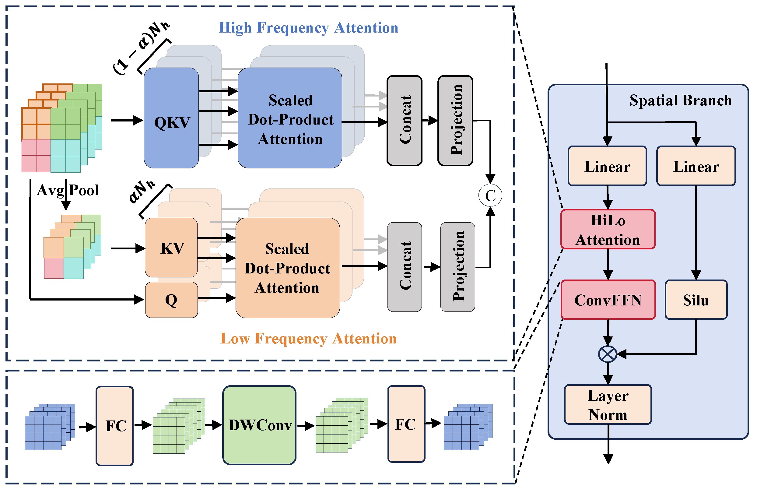
• An improved spatial branch architecture based on ViT is designed to enhance the model’s performance by effectively adjusting the focus on high- and low-frequency information. This design can mitigate the impact of intra-class variability and improves global feature extraction, leading to more robust feature representation.
• The experimental results demonstrate that the proposed method achieves superior performance compared to several representative competitors. This highlights the performance advantages of CPDB-Net.

2. Methodology

2.1. Overview

In hyperspectral image classification (HSIC), increasing the size of hyperspectral image (HSI) patches enhances spatial information but also raises the risk of introducing interference from irrelevant data surrounding the central pixels. To mitigate this, an intuitive and effective approach is to decouple the extraction of central spectral features from the global feature extraction process, thereby protecting the critical central pixel features from being adversely affected.

To achieve this goal, we propose a central pixel-based dual-branch network (CPDB-Net) for HSIC, as illustrated in Figure 1. The network comprises two primary components: a spatial branch and a spectral branch. These branches are designed to extract global spatial features and central spectral features from HSI data for classification purposes. This approach adheres to the widely adopted patch-based classification paradigm in HSIC tasks.

Initially, the HSI patches, derived from the neighboring region of the target pixel to be classified, are used as input. A pointwise convolution (PWConv) is applied for dimensional mapping, unifying the dimensions of the input HSI block to D, facilitating subsequent processing. The mapped HSI patches are then passed through a sequence of operations, including 1 × 1 and 3 × 3 group convolution layers, batch normalization, and a ReLU activation function. These operations extract preliminary features, yielding an initial HSI feature map. Notably, feature extraction is performed only once, without employing multiple stacked layers.

Subsequently, the central region of the HSI feature map is processed by the spectral branch, implemented using CNNs, to extract local spectral features from the central pixels. This preserves the most important spectral information crucial for classification. Simultaneously, the entire feature map is fed into the spatial branch, which utilizes an improved ViT-based architecture incorporating HiLo attention [50]. In the spatial branch, the ViT-based architecture’s long-range modeling capabilities are leveraged, combined with the HiLo attention mechanism for high-low frequency information modulation, enabling the extraction of comprehensive spatial patterns across the entire feature map.

After feature extraction from both branches, global average pooling is applied to each feature map to obtain spectral and spatial features. These features are then concatenated and passed through a fully connected layer to complete the classification task.

2.2. Spectral Branch

The spectral branch primarily leverages the feature extraction capabilities of CNN to mine spectral sequence features from the central pixel region. This focused approach ensures that critical spectral information is captured without interference from surrounding irrelevant data, thereby enhancing classification accuracy. When used solely for classification, this approach is analogous to traditional 1D-CNN classification methods. The design of this component predominantly employs parallel grouped convolutions, enhancing the extraction of multi-scale spectral features by processing different channel groups simultaneously.

Group convolution is a variant of standard convolution that differs in its implementation principles (as illustrated in Figure 2). In traditional convolution, each filter is applied to all input channels, whereas group convolution divides the input channels into separate groups and performs convolution operations independently within each group. This architectural choice offers several advantages in terms of computational efficiency and feature diversity. More specifically, for an input feature map $\mathbf{F}\in {\mathbb{R}}^{C_{\mathrm{in}}\times H\times W}$, $\mathbf{F}$ is first divided into g groups:

$$\mathbf{F}=[{\mathbf{F}}_1,{\mathbf{F}}_2,\cdots ,{\mathbf{F}}_g],{\mathbf{F}}_i\in {\mathbb{R}}^{{\displaystyle \frac{C_{\mathrm{in}}}{g}}\times H\times W},$$

(1)

where g represents the number of groups, and each group ${\mathbf{F}}_i$ has the shape ${\displaystyle \frac{C_{\mathrm{in}}}{g}}\times H\times W$, $[·]$ denotes the concatenation operation along the channel dimension. After grouping, each group of feature maps is assigned convolutional kernels with shapes matching their channel counts, specifically ${\displaystyle \frac{C_{\mathrm{in}}}{g}}\times h\times w$. Each group is allocated an equal number of convolutional kernels, totaling ${\displaystyle \frac{C_{\mathrm{out}}}{g}}$ per group. Upon applying standard convolution operations to each group of feature maps, the resulting feature maps are concatenated to form the final feature map after group convolution:

$${\mathbf{F}}_{\mathrm{output}}=[{\mathbf{F}}_1^{\prime },{\mathbf{F}}_2^{\prime },\cdots ,{\mathbf{F}}_{\mathrm{g}}^{\prime }],{\mathbf{F}}_i^{\prime }\in {\mathbb{R}}^{{\displaystyle \frac{C_{\mathrm{out}}}{g}}\times H\times W},$$

(2)

where ${\mathbf{F}}_{\mathrm{output}}\in {\mathbb{R}}^{C_{\mathrm{out}}\times H\times W}$ is equivalent to that of standard convolution operations but achieves lower computational complexity and more flexible channel allocation strategies.

HSI patches are treated to standardize channel dimensions and extract coarse-grained spectral features. These features are directed to a dual-branch structure, where the central segment of the feature map is processed by the spectral branch using parallel grouped convolutions. The input size is $D^{\prime }\times H^{\prime }\times W^{\prime }$, where $H^{\prime }\times W^{\prime }$ represents the size of the central region of the feature map and $D^{\prime }$ is the embedding dimension. We designed three grouping strategies ($g=4$, $g=8$, $g=16$) to extract multi-scale spectral features. Consequently, three feature maps of size ${\displaystyle \frac{D^{\prime }}{3}}\times H^{\prime }\times W^{\prime }$ are produced, which are then concatenated along the channel dimension, enabling multi-scale spectral feature extraction in the central region,

$${\mathbf{F}}_{\mathrm{spec}}=[{\mathbf{F}}_{\mathrm{gconv}}^{(g=4)},{\mathbf{F}}_{\mathrm{gconv}}^{(g=8)},{\mathbf{F}}_{\mathrm{gconv}}^{(g=16)}]\in {\mathbb{R}}^{D^{\prime }\times H^{\prime }\times W^{\prime }},$$

(3)

where ${\mathbf{F}}_{\mathrm{gconv}}^{(g=n)}$ represents the feature map obtained from group convolution with different values of g. Three distinct granular grouping strategies are utilized to capture spectral features ${\mathbf{F}}_{\mathrm{spec}}$ across different scales, facilitating multi-scale feature extraction within the central spectral region.

2.3. Spatial Branch

To effectively extract global features while mitigating the impact of intra-class variability in an HSI patch, we improved the ViT-based spatial branch by incorporating the HiLo attention mechanism [50], as illustrated in Figure 3. In HSIC, intra-class variability—arising from factors such as varying environmental conditions, lighting, or material properties—poses a significant challenge. The integration of HiLo attention enables the spatial branch to robustly capture both local details and global contextual information, thereby improving classification performance.

The standard ViT architecture comprises three main components: the patch embedding layer, the transformer block, and the task-specific head. The computational process within a transformer block can be described by the following equations:

$$\begin{array}{cc}\hfill {\mathbf{X}}^{\prime }& =\mathbf{X}+\mathrm{MSA}\left(\mathbf{X}\right),\hfill \\ \hfill {\mathbf{X}}^{″}& ={\mathbf{X}}^{\prime }+\mathrm{FFN}\left({\mathbf{X}}^{\prime }\right),\hfill \end{array}$$

(4)

where the input $\mathbf{X}\in {\mathbb{R}}^{N\times D}$ represents a sequence of image patches, with N denoting the number of patches and D representing the embedding dimension. Here, MSA$(·)$ stands for multi-head self-attention, and FFN$(·)$ denotes the feed-forward network.

In the multi-head self-attention (MSA) layer with n attention heads, each head computes the query $\mathbf{Q}$, key $\mathbf{K}$, and value $\mathbf{V}$ matrices through linear transformations of the input $\mathbf{X}$:

$$\mathbf{Q}=\mathbf{X}{\mathbf{W}}_q,\mathbf{K}=\mathbf{X}{\mathbf{W}}_k,\mathbf{V}=\mathbf{X}{\mathbf{W}}_v,$$

(5)

where ${\mathbf{W}}_q$, ${\mathbf{W}}_k$, and ${\mathbf{W}}_v\in {\mathbb{R}}^{D\times D_h}$ are learnable weight matrices, and $D_h$ is the dimensionality of each attention head. The self-attention mechanism for each head is then computed as:

$$\begin{array}{c}{\mathrm{SA}}_h\left(\mathbf{X}\right)=\mathrm{Softmax}\left({\displaystyle \frac{\mathbf{Q}{\mathbf{K}}^{\top }}{\sqrt{D_h}}}\right)\mathbf{V},\\ \mathrm{MSA}\left(\mathbf{X}\right)=[{\mathrm{SA}}_1,\dots ,{\mathrm{SA}}_n]{\mathbf{W}}_o,\end{array}$$

(6)

where ${\mathbf{W}}_o\in {\mathbb{R}}^{(n\times D_h)\times D}$ is a learnable parameter matrix, and $[·]$ denotes the concatenation operation across the channel dimension.

To further enhance the spatial branch’s capability to capture global features, we integrated the HiLo attention mechanism, which comprises two components: high-frequency attention and low-frequency attention. Prior to computing attention, the image patches are partitioned into local windows of size ${\displaystyle \frac{H_p}{w}}\times {\displaystyle \frac{W_p}{w}}$, where $H_p\times W_p$ denotes the dimensions of the image patches, and w represents the window size. The high-frequency attention component applies multi-head self-attention within these local windows to capture detailed local image features. Conversely, the low-frequency attention component performs average pooling on the local windows, downsampling the image patches to ${\displaystyle \frac{H_p}{w}}\times {\displaystyle \frac{W_p}{w}}$. Subsequently, the key $\mathbf{K}$ and value $\mathbf{V}$ matrices are computed on the downsampled images, allowing the attention mechanism to focus more effectively on low-frequency image features. Importantly, the total number of attention heads is shared between high-frequency and low-frequency attention, with the allocation regulated by a parameter $\mathbf{\alpha }$. The low-frequency component of HiLo attention utilizes average pooling to downsample the image, thereby smoothing spectral differences. By adjusting the ratio of high-frequency to low-frequency information, the spatial branch’s ability to extract robust global features is significantly enhanced.

3. Results

3.1. Datasets Description

The performance of the proposed CPDB-Net method will be evaluated on three widely used datasets in the field of hyperspectral image classification: Indian Pines, Pavia University, and Houston 2013.

3.1.1. Indian Pines

The Indian Pines dataset was collected by an Airborne Visible/Infrared Imaging Spectrometer (AVIRIS) in June 1992, focusing on agricultural regions in Northwestern Indiana, USA. It contains 145 × 145 pixels with a spatial resolution of 20 × 20 m and 220 spectral bands spanning from 400 to 2500 nm. In order to maintain the integrity of the data, 20 spectral bands were excluded, resulting in a final dataset containing 200 bands for further analysis. The dataset is renowned for its diverse vegetation types and varying soil conditions, making it a commonly used benchmark for hyperspectral image classification. Figure 4 presents the false color and ground-truth maps, and

Table 1. Land cover classes and numbers of samples in the Indian Pines dataset.

No.	Class Name	Training Samples	Test Samples	Total Samples
1	Alfalfa	20	26	46
2	Corn-notill	20	1408	1428
3	Corn-mintill	20	810	830
4	Corn	20	217	237
5	Grass-pasture	20	463	483
6	Grass-trees	20	710	730
7	Grass-pasture-mowed	20	8	28
8	Hay-windrowed	20	458	478
9	Oats	15	5	20
10	Soybean-notill	20	952	972
11	Soybean-mintill	20	2435	2455
12	Soybean-clean	20	573	593
13	Wheat	20	185	205
14	Woods	20	1245	1265
15	Buildings-Grass-Trees	20	366	386
16	Stone-Steel-Towers	20	73	93
Total		315	9934	10,249

provides the allocation of training and testing samples across the different classes.

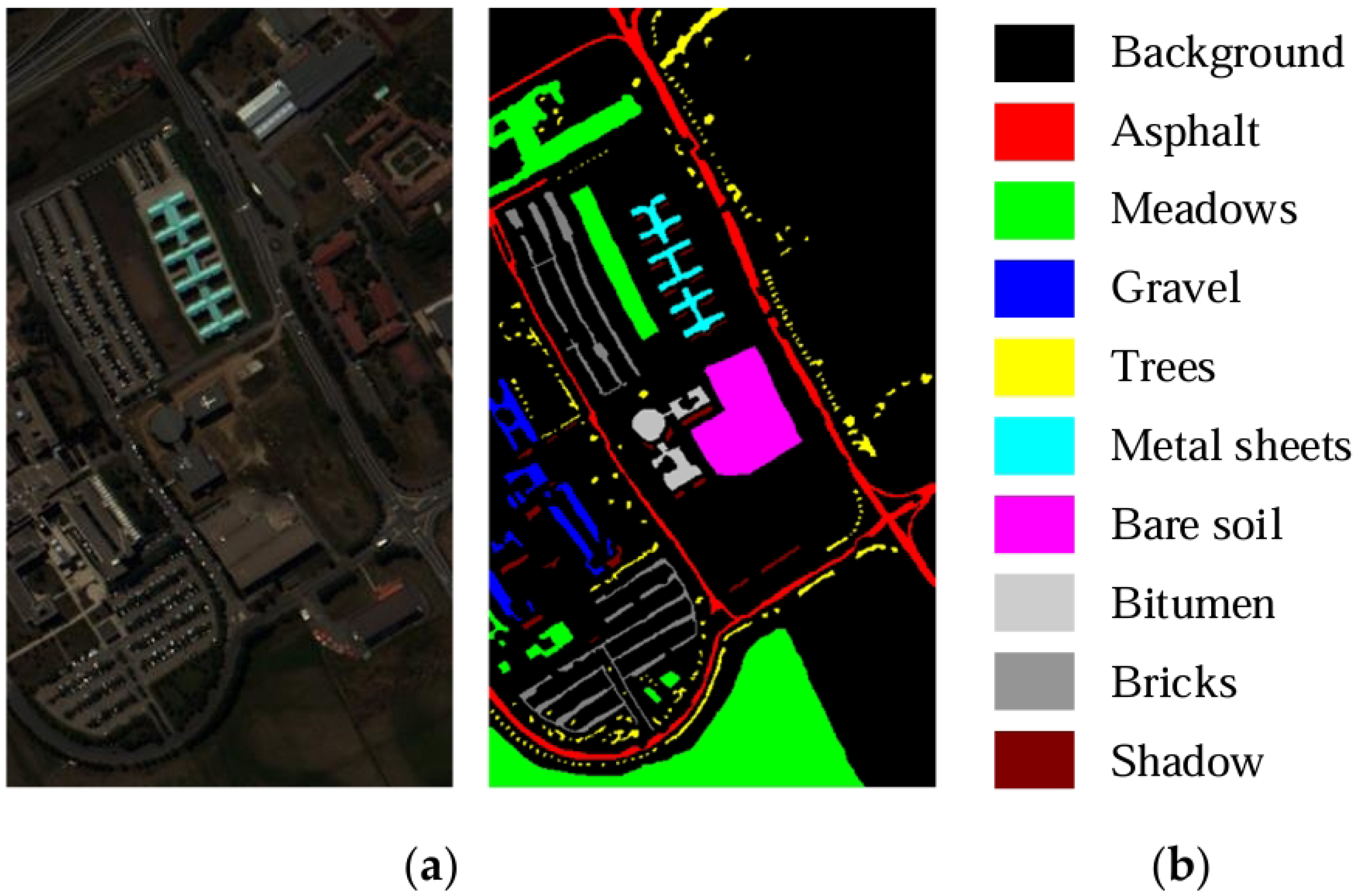
3.1.2. Pavia University

The Pavia University dataset was acquired by the Reflective Optics System Imaging Spectrometer (ROSIS) sensor over the University of Pavia, Italy. This dataset comprises 610 × 340 pixels with a high spatial resolution of 1.3 × 1.3 m and includes 103 spectral bands ranging from 430 to 860 nm. The dataset features nine land cover classes, such as buildings, trees, roads, bare soil, and water, representing a variety of urban materials and structures. This diversity facilitates the evaluation of hyperspectral classifiers in distinguishing between different urban land cover types based on their spectral characteristics. Figure 5 presents the false color and ground-truth maps, whereas

Table 2. Land cover classes and numbers of samples in the Pavia University dataset.

No.	Class Name	Training Samples	Test Samples	Total Samples
1	Asphalt	20	6611	6631
2	Meadows	20	18,629	18,649
3	Gravel	20	2079	2099
4	Trees	20	3044	3064
5	Mental sheets	20	1325	1345
6	Bare soil	20	5009	5029
7	Bitumen	20	1310	1330
8	Bricks	20	3662	3682
9	Shadow	20	927	947
Total		180	42,596	42,776

outlines the allocation of training and testing samples across each class.

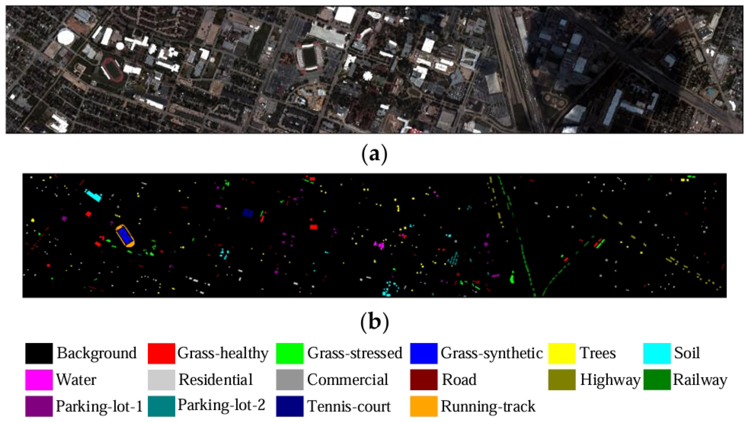
3.1.3. Houston 2013

The Houston dataset centers on an urban region near the University of Houston campus, USA. It was acquired by the National Center for Airborne Laser Mapping (NCALM) for the 2013 IEEE GRSS Data Fusion Contest [51]. It consists of 349 × 1905 pixels with a spatial resolution of 2.5 × 2.5 m and includes 144 spectral bands ranging from 380 to 1050 nm. This dataset features a rich variety of urban materials, such as asphalt, concrete, vegetation, and water bodies, under diverse environmental conditions. The Houston 2013 dataset is renowned for its complexity and diversity, presenting significant challenges for hyperspectral image classification methods. Figure 6 presents the true color and ground-truth maps, whereas

Table 3. Land cover classes and numbers of samples in the Houston 2013 dataset.

No.	Class Name	Training Samples	Test Samples	Total Samples
1	Grass-healthy	20	1231	1251
2	Grass-stressed	20	1234	1254
3	Grass-synthetic	20	677	697
4	Tree	20	1224	1244
5	Soil	20	1222	1242
6	Water	20	305	325
7	Residential	20	1248	1268
8	Commercial	20	1224	1244
9	Road	20	1232	1252
10	Highway	20	1207	1227
11	Railway	20	1215	1235
12	Parking-lot-1	20	1213	1233
13	Parking-lot-2	20	449	469
14	Tennis-court	20	4008	428
15	Running-track	20	640	660
Total		300	14,729	15,029

provides the allocation of training and testing samples across the different classes.

3.2. Experimental Setup

To objectively evaluate the performance of the proposed CPDB-Net, several representative methods in the HSIC field were selected for comparison:

• SSRN [31]: A CNN-based hyperspectral image classification (HSIC) algorithm. Its innovative integration of skip connections within the 3D-CNN architecture has established SSRN as a classic CNN-based method, leading to extensive citations in numerous subsequent studies.
• DBDA [52]: A CNN-based algorithm that employs a dual-branch structure, with each branch dedicated to extracting spatial and spectral features, respectively. This method demonstrates superior performance under limited training samples and has inspired numerous dual-branch designs.
• LSFAT [40]: An algorithm built on the ViT architecture, which has showcased substantial potential in tackling the HSIC problem and is becoming a classic approach in ViT-based methods.
• SSFTT [53]: A representative ViT-based method that improves the patching strategy for spectral information. Its innovative design has been widely recognized and frequently cited in the field.
• CT-Mixer [54]: A state-of-the-art hybrid architecture that integrates CNN and ViT structures. By effectively combining their respective strengths, CT-Mixer achieves competitive performance and serves as a representative work of CNN–ViT hybrid approaches.
• SS-Mamba [55]: Employs a dual-branch spatial-spectral architecture based on the recent Mamba model [56] for hyperspectral image classification. This innovative approach leverages Mamba’s strengths, resulting in outstanding classification performance.

The aforementioned methods encompass CNN, ViT, and CNN–ViT hybrid architectures, as well as the latest approaches based on the Mamba model, providing a comprehensive basis for comparison.

In the experimental setup, the input HSI patch size is set to $27\times 27$ (i.e., $H=W=27$). In the spatial branch, patch embedding is performed using a $3\times 3$ convolutional layer, reducing the input to a $9\times 9$ feature map to mitigate excessive computational load. Furthermore, in the spectral branch, only the central $3\times 3$ region is utilized as input. The spectral mapping and embedding dimensions are configured to 128 and 96, respectively. For optimization, the Adam optimizer was employed with an initial learning rate of 0.001 and a weight decay of 0.0001. A cosine annealing learning rate scheduler was utilized, with $T_0$ set to 5 and $T_{\mathrm{mult}}$ set to 2. During training, we performed 10 random splits of the dataset into training and testing samples. Each split was trained for 300 epochs, and the test results were averaged to evaluate the classification performance. Additionally, the attention head allocation ratio $\alpha$ was set to 0.4 for the Pavia University dataset and 0.6 for the other datasets. The hyperparameters mentioned above were initially set based on experience and were further fine-tuned according to experimental results.

The classification methods were evaluated using overall accuracy (OA), average accuracy (AA), and the Kappa coefficient (Kappa) as key performance metrics. To ensure stable and consistent results, each experiment was repeated ten times with different random initializations. In each independent iteration, training samples were randomly selected from the complete set of labeled data.

3.3. Ablation Experiment

To evaluate the effectiveness of the proposed spectral and spatial branches, we conducted ablation studies on three datasets: Indian Pines, Pavia University, and Houston 2013. The ablation experiments were designed to assess the individual and combined contributions of the central spectral branch and the improved spatial branch to the overall performance of the proposed CPDB-Net. Here, “Base” refers to the original ViT architecture as the spatial branch, “Spectral Branch” refers to the CNN-based central spectral branch alone, “Base+Spectral Branch” indicates the combination of the central spectral branch with the base spatial branch, and “Ours” refers to the complete version of the proposed CPDB-Net, which simultaneously utilizes the central spectral branch and the improved spatial branch, incorporating HiLo attention for classification. The results of the ablation experiments, presented in

Table 4. Ablation experiment on the Indian Pines dataset.

Metrics	Base	Spectral Branch	Base + Spectral Branch	Ours
OA (%)	88.99 ± 1.30	85.34 ± 1.54	92.00 ± 1.52	92.67 ± 1.42
AA (%)	93.80 ± 0.75	92.59 ± 0.77	95.87 ± 0.72	96.15 ± 0.66
Kappa (%)	87.50 ± 1.46	83.41 ± 1.60	90.88 ± 1.70	91.64 ± 1.61

Bold values denote the best performance.

,

Table 5. Ablation experiment on the Pavia University dataset.

Metrics	Base	Spectral Branch	Base + Spectral Branch	Ours
OA (%)	95.39 ± 2.30	90.85 ± 2.33	96.57 ± 2.28	97.48 ± 1.68
AA (%)	97.02 ± 1.25	93.94 ± 1.01	98.31 ± 0.84	98.66 ± 0.65
Kappa (%)	93.98 ± 2.96	88.13 ± 2.94	95.52 ± 2.93	96.70 ± 2.18

Bold values denote the best performance.

and

Table 6. Ablation experiment on the Houston 2013 dataset.

Metrics	Base	Spectral Branch	Base + Spectral Branch	Ours
OA (%)	93.68 ± 1.08	84.82 ± 5.30	94.71 ± 0.90	95.02 ± 0.85
AA (%)	94.42 ± 0.88	86.70 ± 4.79	95.39 ± 0.73	95.67 ± 0.71
Kappa (%)	93.16 ± 1.16	83.60 ± 5.73	94.28 ± 0.97	94.61 ± 0.92

Bold values denote the best performance.

, consistently demonstrate the effectiveness of the proposed central pixel dual-branch structure and the improved spatial branch structure across all three datasets.

Taking the Pavia University dataset as an example (Table 5), the proposed CPDB-Net significantly outperforms the “Base” model, with improvements of 2.09%, 1.64%, and 2.72% in OA, AA, and Kappa, respectively. These results highlight the importance of incorporating both the central spectral branch and the improved spatial branch for accurate classification. Moreover, CPDB-Net achieves substantial enhancements over the “Spectral Branch” model, with increases of 6.63%, 4.72%, and 8.57% in OA, AA, and Kappa, respectively. The “Base+Spectral Branch” model, which combines the central spectral branch with the base spatial branch, also exhibits notable improvements over the individual “Base” and “Spectral Branch” models. These results underscore the complementary nature of the spectral and spatial branches and the benefits of their integration.

Further analysis reveals that the complete CPDB-Net outperforms the “Base+Spectral Branch” model, with improvements of 0.91%, 0.35%, and 1.18% in OA, AA, and Kappa, respectively. This comparison highlights the effectiveness of the HiLo attention mechanism incorporated in the improved spatial branch, which enhances the model’s ability to capture both high-frequency details and low-frequency global contextual information to further mitigate the impact of intra-class variability.

The ablation study results on the Indian Pines and Houston 2013 datasets (Table 4 and Table 6) exhibit similar trends, confirming the generalizability and robustness of the proposed CPDB-Net across different datasets.

3.4. Comparative Experiments

To comprehensively evaluate the effectiveness of CPDB-Net,

Table 7. Classification results (mean ± standard deviation) on the Indian Pines dataset.

Class	SSRN	DBDA	LSFAT	SSFTT	CT-Mixer	SS-Mamba	Ours
1	86.04 ± 9.73	79.35 ± 12.80	100.0 ± 0.00	100.0 ± 0.00	100.0 ± 0.00	100.0 ± 0.00	100.0 ± 0.00
2	86.85 ± 6.00	86.89 ± 10.74	81.13 ± 6.11	85.38 ± 3.92	81.94 ± 3.95	80.30 ± 4.58	83.40 ± 3.78
3	86.54 ± 5.65	86.88 ± 8.79	86.90 ± 5.32	87.63 ± 5.69	87.47 ± 4.29	88.54 ± 5.07	91.77 ± 6.09
4	73.29 ± 13.10	81.64 ± 11.47	99.07 ± 1.23	98.06 ± 2.43	99.35 ± 1.11	99.49 ± 0.76	98.89 ± 1.15
5	98.00 ± 1.96	97.02 ± 3.74	92.89 ± 2.90	94.15 ± 2.09	93.24 ± 1.54	93.69 ± 1.99	95.01 ± 1.55
6	97.79 ± 1.40	96.54 ± 1.25	95.35 ± 3.89	97.98 ± 1.26	95.30 ± 3.47	98.34 ± 1.53	98.83 ± 1.79
7	73.78 ± 18.70	58.08 ± 28.22	100.0 ± 0.00	100.0 ± 0.00	100.0 ± 0.00	100.0 ± 0.00	100.0 ± 0.00
8	99.46 ± 0.83	99.62 ± 0.58	99.56 ± 0.97	99.34 ± 1.22	99.98 ± 0.07	100.0 ± 0.00	99.97 ± 0.06
9	44.13 ± 20.56	32.65 ± 11.22	100.0 ± 0.00	100.0 ± 0.00	100.0 ± 0.00	100.0 ± 0.00	100 ± 0.00
10	79.53 ± 6.45	81.08 ± 8.08	87.58 ± 4.89	89.66 ± 4.47	87.88 ± 4.44	89.61 ± 3.92	90.69 ± 4.30
11	92.94 ± 3.50	95.43 ± 4.19	85.26 ± 3.98	84.72 ± 5.24	86.89 ± 3.17	89.51 ± 5.87	89.67 ± 4.21
12	82.78 ± 10.73	90.57 ± 13.45	83.70 ± 4.94	77.40 ± 4.99	82.57 ± 6.87	93.32 ± 4.74	92.63 ± 4.13
13	95.49 ± 3.82	91.42 ± 5.35	99.89 ± 0.32	98.86 ± 2.15	98.97 ± 1.89	99.46 ± 1.62	99.78 ± 0.64
14	97.87 ± 1.14	98.43 ± 1.05	97.69 ± 1.18	98.75 ± 1.18	97.07 ± 1.48	98.63 ± 1.40	99.39 ± 0.95
15	87.30 ± 7.75	88.99 ± 5.46	95.63 ± 3.74	96.91 ± 2.02	96.97 ± 2.59	96.67 ± 3.16	99.09 ± 0.93
16	79.51 ± 4.48	68.09 ± 12.75	98.49 ± 1.67	100.0 ± 0.00	99.59 ± 0.63	99.73 ± 0.82	99.31 ± 0.68
OA (%)	89.44 ± 1.38	90.26 ± 3.06	89.35 ± 1.38	90.10 ± 1.58	89.87 ± 1.28	91.59 ± 1.85	92.67 ± 1.42
AA (%)	85.08 ± 2.08	83.29 ± 2.47	93.95 ± 0.62	94.30 ± 0.83	94.20 ± 0.72	95.46 ± 0.90	96.15 ± 0.66
Kappa (%)	88.00 ± 1.55	88.95 ± 3.43	87.90 ± 1.55	88.76 ± 1.78	88.49 ± 1.44	90.42 ± 2.08	91.64 ± 1.61

Bold values denote the best performance.

,

Table 8. Classification results (mean ± standard deviation) on the Pavia University dataset.

Class	SSRN	DBDA	LSFAT	SSFTT	CT-Mixer	SS-Mamba	Ours
1	97.84 ± 1.71	98.74 ± 1.20	87.16 ± 3.78	86.16 ± 6.15	90.59 ± 5.26	95.70 ± 3.41	96.52 ± 2.52
2	97.72 ± 0.81	99.51 ± 0.36	95.05 ± 3.17	94.50 ± 3.60	94.62 ± 4.88	94.05 ± 4.27	96.21 ± 3.63
3	83.71 ± 8.17	90.81 ± 12.10	93.95 ± 4.43	93.94 ± 4.13	94.39 ± 4.19	99.61 ± 0.54	97.77 ± 4.11
4	97.70 ± 2.01	92.74 ± 7.92	92.76 ± 4.46	88.97 ± 5.25	84.61 ± 6.80	98.92 ± 0.55	98.46 ± 0.94
5	99.86 ± 0.27	99.53 ± 0.63	98.85 ± 0.89	98.95 ± 1.06	99.18 ± 0.67	100.0 ± 0.00	100.0 ± 0.00
6	91.98 ± 3.69	90.96 ± 5.45	99.19 ± 0.82	96.07 ± 3.90	99.53 ± 1.08	99.19 ± 1.63	99.57 ± 0.73
7	88.49 ± 12.03	93.80 ± 8.83	99.08 ± 0.76	99.58 ± 0.67	99.34 ± 0.67	99.93 ± 0.20	99.99 ± 0.02
8	84.79 ± 7.36	89.83 ± 6.47	91.74 ± 3.98	86.63 ± 7.99	97.10 ± 2.75	98.50 ± 0.95	99.43 ± 0.47
9	99.41 ± 0.94	96.82 ± 1.69	95.49 ± 2.30	95.54 ± 2.17	93.95 ± 3.14	99.96 ± 0.05	100.0 ± 0.00
OA (%)	94.72 ± 1.17	95.87 ± 1.85	94.06 ± 1.29	92.61 ± 1.92	94.33 ± 2.85	96.40 ± 2.27	97.48 ± 1.68
AA (%)	93.50 ± 2.07	94.75 ± 2.36	94.81 ± 0.54	93.37 ± 1.24	94.81 ± 1.77	98.43 ± 0.77	98.66 ± 0.65
Kappa (%)	93.02 ± 1.53	94.58 ± 2.41	92.22 ± 1.63	90.29 ± 2.47	92.60 ± 3.63	95.31 ± 2.92	96.70 ± 2.18

Bold values denote the best performance.

and

Table 9. Classification results (mean ± standard deviation) on the Houston 2013 University dataset.

Class	SSRN	DBDA	LSFAT	SSFTT	CT-Mixer	SS-Mamba	Ours
1	96.25 ± 2.94	93.48 ± 5.59	92.67 ± 4.33	95.36 ± 3.62	90.90 ± 5.13	92.88 ± 4.33	93.81 ± 4.21
2	97.65 ± 2.48	95.10 ± 3.78	97.57 ± 1.98	98.58 ± 1.13	95.11 ± 2.60	95.99 ± 2.91	97.88 ± 2.17
3	99.93 ± 0.22	100.0 ± 0.00	98.17 ± 1.20	99.20 ± 0.60	97.10 ± 4.20	100.0 ± 0.00	100.0 ± 0.00
4	95.98 ± 4.13	97.13 ± 2.17	96.58 ± 1.78	97.82 ± 3.19	92.27 ± 4.20	99.17 ± 1.67	99.17 ± 1.68
5	95.41 ± 2.36	97.66 ± 2.42	99.78 ± 0.29	99.99 ± 0.02	98.58 ± 3.08	98.29 ± 5.08	98.96 ± 3.09
6	97.31 ± 7.83	97.37 ± 2.23	97.47 ± 3.66	98.42 ± 3.86	96.42 ± 3.53	96.39 ± 3.63	96.39 ± 3.97
7	92.10 ± 2.47	91.93 ± 3.62	86.43 ± 2.43	84.32 ± 5.32	89.18 ± 3.91	91.60 ± 2.06	93.18 ± 1.78
8	93.23 ± 3.49	94.88 ± 3.19	83.25 ± 6.19	80.80 ± 5.19	83.90 ± 4.83	83.33 ± 4.35	82.87 ± 4.00
9	89.87 ± 3.83	88.57 ± 2.27	82.61 ± 5.52	78.82 ± 6.79	86.58 ± 2.31	92.05 ± 2.02	93.77 ± 3.14
10	86.49 ± 6.78	89.76 ± 3.83	96.50 ± 2.86	95.10 ± 3.33	99.09 ± 1.52	98.05 ± 1.94	99.09 ± 0.84
11	90.45 ± 1.94	95.44 ± 2.10	93.46 ± 5.38	95.82 ± 3.23	92.34 ± 6.17	92.48 ± 6.14	94.06 ± 5.66
12	89.91 ± 4.73	93.15 ± 3.27	89.55 ± 5.62	89.65 ± 4.87	91.27 ± 5.74	91.24 ± 5.57	89.54 ± 5.89
13	93.52 ± 5.65	82.75 ± 6.06	92.98 ± 4.01	97.75 ± 2.10	91.22 ± 5.39	92.87 ± 3.30	96.43 ± 2.21
14	97.67 ± 3.29	98.13 ± 2.59	99.88 ± 0.25	99.85 ± 0.22	100.0 ± 0.00	100.0 ± 0.00	100.0 ± 0.00
15	96.93 ± 1.96	95.05 ± 2.47	99.97 ± 0.09	100.0 ± 0.00	98.63 ± 2.38	100.0 ± 0.00	99.98 ± 0.04
OA (%)	93.32 ± 1.05	93.67 ± 0.92	92.85 ± 0.93	92.88 ± 0.97	92.73 ± 1.21	94.30 ± 1.10	95.02 ± 0.85
AA (%)	94.18 ± 1.12	94.03 ± 0.87	93.79 ± 0.74	94.10 ± 0.85	93.51 ± 1.04	94.96 ± 0.89	95.67 ± 0.71
Kappa (%)	92.78 ± 1.13	93.16 ± 1.00	92.27 ± 1.01	92.30 ± 1.05	92.14 ± 1.31	93.84 ± 1.20	94.61 ± 0.92

present the classification performance of the proposed method alongside selected benchmark methods on the Indian Pines, Pavia University, and Houston 2013 datasets. The experimental results demonstrate consistent superiority across all three metrics (OA, AA, Kappa). The significant performance improvements validate the effectiveness of our dual-branch design in preserving crucial central pixel information while leveraging global contextual features. Specifically, on the Indian Pines dataset, CPDB-Net improves OA by 3.23%, AA by 11.07%, and Kappa by 3.64% compared with the CNN-based representative method SSRN. Compared with the ViT-based method SSFTT, it enhances OA by 2.57%, AA by 1.85%, and Kappa by 2.88%. Compared with the hybrid architecture method CT-Mixer, CPDB-Net achieves increases of 2.8% in OA, 1.95% in AA, and 3.15% in Kappa. Even when compared with the latest Mamba-based method SS-Mamba, CPDB-Net improves OA by 0.88%, AA by 0.69%, and Kappa by 1.22%.

Further analysis reveals an interesting finding: ViT-based and hybrid methods do not consistently outperform CNN-based approaches across all three datasets. Specifically, on the Indian Pines dataset, SSFTT and CT-Mixer achieve increases in OA of 0.66% and 0.43%, respectively, compared with SSRN. However, on the Pavia University dataset, SSFTT and CT-Mixer result in decreases in OA by 2.11% and 0.39%, respectively, relative to SSRN. Similarly, on the Houston 2013 dataset, SSFTT and CT-Mixer show reductions in OA by 0.44% and 0.59%, respectively, compared with SSRN. This performance inconsistency is likely due to the relatively complex architectures of these methods, which may not perform optimally with a limited number of samples. This observation further justifies our motivation to design a specialized dual-branch architecture rather than simply combining CNN and ViT.

It is worth noting that SS-Mamba, using the latest Mamba architecture, achieves highly powerful classification performance. Nevertheless, our proposed CPDB-Net surpasses SS-Mamba with improvements of 1.08% in OA, 0.69% in AA, and 1.22% in Kappa on the Indian Pines dataset, and also demonstrates performance gains on the Pavia University and Houston 2013 datasets. These consistent improvements across different datasets demonstrate the robustness of our CPDB-Net in handling spectral variability. CPDB-Net exhibits competitive effectiveness compared with the latest Mamba model.

To provide qualitative analysis, Figure 7, Figure 8 and Figure 9 present visualizations of the classification results across different datasets. The visual comparison shows that our method achieves more complete and consistent performance along the edges of similar land cover classes compared to the baseline methods. This superior boundary preservation ability particularly validates our dual-branch design in reducing spatial interference. Particularly, in Figure 7, within the upper rear and slightly lower central regions, our method exhibits fewer errors at the boundaries of large aggregated areas of the same land cover class. In Figure 8, where the land cover shapes are highly irregular, our method demonstrates superior ability in handling dispersed land covers and edge regions. These visualization results strongly support the effectiveness of the central pixel dual-branch structure.

3.5. Parameter Analysis

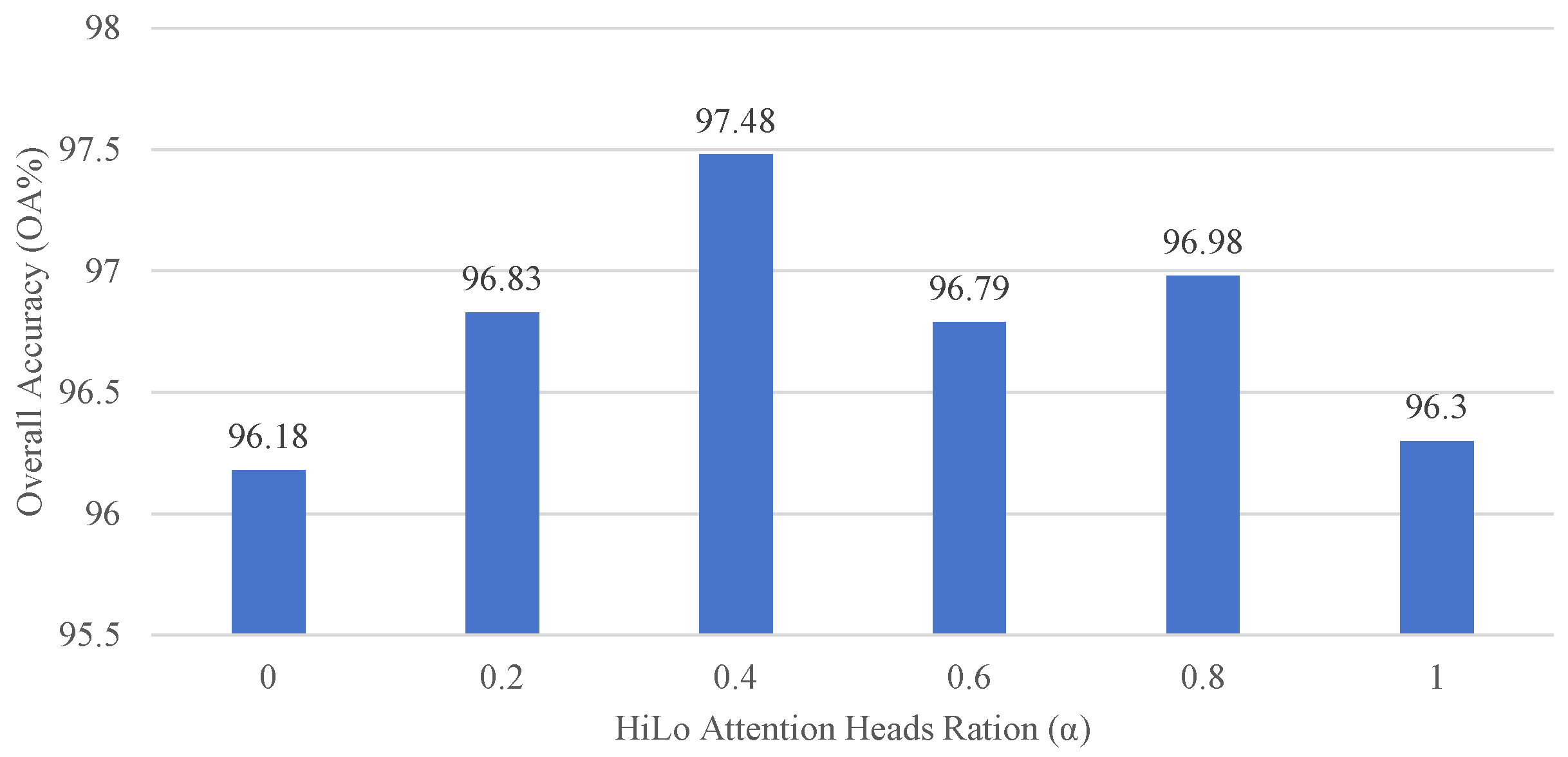
To investigate the key parameters of the proposed algorithm, experiments were conducted on the Pavia University dataset. Figure 10 presents the experimental results for different allocation ratios $\alpha$ of high and low-frequency attention heads in HiLo attention, which is varied from 0 to 1 with a step size of 0.2. It is important to note that the classification performance is suboptimal when $\alpha$ is set to extreme values (0 or 1). This can be attributed to the fixed local window size, which does not guarantee that all pixels within the window belong to the same category. Consequently, placing excessive emphasis on low-frequency attention can lead to the extraction of non-representative features. Conversely, focusing too much on high-frequency attention is akin to merely windowing the original ViT, which constrains its ability to capture global features. Therefore, a moderate value of $\alpha$ yields superior performance by effectively leveraging both high and low-frequency information.

Another key parameter in the proposed method is the size of the central spectral branch. To analyze its impact on classification performance, experiments were conducted with the central region size ranging from 3 × 3 to 9 × 9, with a step size of 2. Figure 11 shows the experimental results for different sizes of the central spectral branch. A clear trend can be observed: as the size of the central region increases, the classification accuracy exhibits a corresponding decrease. This phenomenon can be explained by the fact that larger central regions are more prone to interference from neighboring pixels, which can negatively impact the critical central pixel features essential for accurate classification. Consequently, employing a smaller central pixel region proves to be more effective in achieving optimal classification performance, as it minimizes the influence of potentially irrelevant or misleading information from the surrounding context.

To further explore the effectiveness of the group convolution strategy employed in the Spectral Branch, grouping strategies experiments were conducted.

Table 10. Comparison of different grouping strategies on the Pavia University dataset.

Group Configurations	OA (%)	AA (%)	Kappa (%)
$(g=4,4,4)$	96.28 ± 2.40	98.11 ± 1.15	95.15 ± 3.09
$(g=8,8,8)$	96.18 ± 1.79	98.24 ± 0.71	95.01 ± 2.31
$(g=16,16,16)$	96.41 ± 2.54	98.18 ± 1.00	95.32 ± 3.28
$(g=2,4,8)$	97.24 ± 1.95	98.54 ± 0.78	96.38 ± 2.52
$(g=8,16,32)$	96.96 ± 2.15	98.51 ± 0.65	96.03 ± 2.78
$(g=4,8,16)$	97.48 ± 1.68	98.66 ± 0.65	96.70 ± 2.18

Bold values denote the best performance.

illustrates the performance differences of CPDB-Net on the Pavia University dataset using various grouping strategies. The results reveal that there is a notable distinction between multi-scale group convolutions and standard group convolutions (for instance, g = 4, 8, 16 compared to g = 8, 8, 8). Within each category, whether multi-scale or standard, the performance variations among different group configurations are relatively minor. This indicates that multi-scale group convolutions can enhance the CNN’s ability to extract central spectral features more effectively. Additionally, it was observed that even the least effective strategy (g = 8, 8, 8) achieved an overall accuracy (OA) improvement of 0.81% over the “Base” method presented in Table 5. This observation underscores that even when the CNN branch performs suboptimally, it remains effective within a center pixel-based dual-branch framework, thereby reinforcing the efficacy of this structural design.

Additionally, experiments with varying sample sizes were set up to evaluate the robustness of our method under extreme data conditions. Specifically, experiments were performed on the Pavia University dataset using 1, 5, 10, and 15 samples per class. Notably, our approach demonstrates strong performance even under relatively limited settings (20 samples per class). However, as Figure 12 indicates, there is a significant performance drop with extremely scarce samples. This highlights the need for future exploration into specialized few-shot and unsupervised techniques to further enhance robustness in data-scarce scenarios.

3.6. Computational Efficiency Analysis

Computational efficiency analysis remains a critical component for evaluating model performance, as high computational efficiency directly correlates with a model’s practical deployment potential. Computational efficiency is assessed using three metrics: Params (parameter count), FLOPs (floating-point operations), and MACs (multiply-accumulate operations), with lower values generally indicating superior performance. As shown in

Table 11. Comparison of computational efficiency and OA on the Pavia University dataset. Lower Params, FLOPs, and MACs (↓) are better; higher OA (↑) is better.

Model	Params (M) ↓	FLOPs (G) ↓	MACs (G) ↓	OA (%) ↑
SSFTT	0.93	0.51	1.02	92.61
CT-mixer	0.61	0.45	0.90	94.33
SS-Mamba	0.99	0.26	0.52	96.40
Ours	0.26	0.04	0.08	97.48

Bold values denote the best performance.

, our proposed method achieves both the highest performance (highest OA score) and significant computational efficiency advantages over comparable methods. Specifically, compared to the CNN–ViT hybrid model CT-Mixer, CPDB-Net reduces parameters by 0.35 million and achieves 0.41 fewer FLOPs. When benchmarked against the computation-efficient state-of-the-art method SS-Mamba, our model further demonstrates a reduction of 0.73 million parameters and 0.22 fewer FLOPs. These performance gains stem from the model’s streamlined architecture design and the incorporation of effective intuitive priors, thereby reinforcing the value and practicality of CPDB-Net.

4. Discussion

4.1. Results Interpretation and Discussion

The proposed CPDB-Net demonstrates superior performance in HSIC across the Indian Pines, Pavia University, and Houston 2013 datasets, achieving the highest overall accuracies of 92.67%, 97.48%, and 95.02%, respectively. These results surpass those of several established methods, highlighting the effectiveness of integrating CNN with ViT in a dual-branch architecture. The superior performance arises from two main aspects that have been insufficiently addressed in other methods:

• The central pixel-based dual-branch architecture effectively separates the central spectral feature extraction from the global spatial processing. This separation mitigates the interference of irrelevant information and addresses the issue of intra-class spectral variability, thereby enhancing both the robustness and generalization capabilities of the model.
• The spatial information extraction branch enhanced by the HiLo attention mechanism adjusts the balance between high- and low-frequency attention. This adjustment ensures that intra-class spectral variations are smoothed while retaining detailed high-frequency spectral features, thereby enhancing the capability for global feature extraction.

The quantitative analyses presented in the ablation experiments and parameter analysis in Section 3 substantiate the effectiveness of the aforementioned contributions. Additionally, the visualization results reveal that in edge regions and isolated areas where background pixel interference is significant, the classification outcomes of the proposed method are more complete and exhibit higher accuracy compared with the other methods. These observations are consistent with the analytical results previously discussed, demonstrating the robustness and generalization capabilities of the CPDB-Net in various complex scenarios, particularly in cases with high spectral variability and mixed spatial information.

4.2. Limitations and Future Work

The CPDB-Net has demonstrated robust performance across various complex hyperspectral image classification scenarios, particularly in cases with high spectral variability and mixed spatial information. However, there remain several promising avenues for future research to further enhance its performance and applicability.

One potential direction is to explore the development of learnable methods that dynamically extract and integrate spatial information from the surrounding context. While the current dual-branch architecture effectively separates central pixel spectral features based on a prior assumption, exploring learnable methods that dynamically extract and integrate spatial information could lead to further improvements in classification accuracy. Such learnable approaches could potentially strike an optimal balance between preserving central pixel information and leveraging relevant contextual cues, thereby enhancing the model’s robustness and generalization capabilities.

Furthermore, integrating graph convolutional networks (GCNs) into the framework offers another critical avenue for spatial modeling improvements. GCNs excel at capturing non-local spatial dependencies and contextual patterns in hyperspectral data, which are often missed by traditional convolutional methods. For instance, GCN-based approaches can explicitly model the graph structure of pixel neighborhoods to propagate spectral-spatial features across the image manifold. Incorporating such mechanisms could complement the current spatial branch of CPDB-Net, enabling more nuanced exploitation of spatial correlations and reducing intra-class variability.

Another area for future improvement is the frequency-aware HiLo attention mechanism introduced in the spatial branch. Although this approach has shown promise in reducing intra-class spectral variability and preserving high-frequency spectral details, there is still room for further refinement. Future work could explore more advanced frequency decomposition techniques to better capture and leverage the discriminative information present in different frequency bands. Additionally, investigating dynamic mechanisms for adjusting the balance between high- and low-frequency information could further enhance the adaptability and performance of the model.

In conclusion, we believe that the proposed framework can be further strengthened to tackle even more complex and diverse hyperspectral image classification tasks in the future. These promising research directions highlight the potential for CPDB-Net to continue advancing the state of the -art in hyperspectral image classification and contribute to the development of more accurate, robust, and efficient classification methods.

References

1. Lu, B.; Dao, P.; Liu, J.; He, Y.; Shang, J. Recent Advances of Hyperspectral Imaging Technology and Applications in Agriculture. Remote Sens. 2020, 12, 2659. [Google Scholar] [CrossRef]
2. Yu, C.; Zhao, X.; Gong, B.; Hu, Y.; Song, M.; Yu, H.; Chang, C.I. Distillation-Constrained Prototype Representation Network for Hyperspectral Image Incremental Classification. IEEE Trans. Geosci. Remote Sens. 2024, 62, 5507414. [Google Scholar] [CrossRef]
3. Camps-Valls, G.; Tuia, D.; Bruzzone, L.; Benediktsson, J.A. Advances in hyperspectral image classification: Earth monitoring with statistical learning methods. IEEE Signal Process. Mag. 2013, 31, 45–54. [Google Scholar] [CrossRef]
4. Peyghambari, S.; Zhang, Y. Hyperspectral remote sensing in lithological mapping, mineral exploration, and environmental geology: An updated review. J. Appl. Remote Sens. 2021, 15, 031501. [Google Scholar] [CrossRef]
5. Murphy, R.J.; Schneider, S.; Monteiro, S.T. Consistency of Measurements of Wavelength Position From Hyperspectral Imagery: Use of the Ferric Iron Crystal Field Absorption at 900 nm as an Indicator of Mineralogy. IEEE Trans. Geosci. Remote Sens. 2013, 52, 2843–2857. [Google Scholar] [CrossRef]
6. Yan, L.; Zhao, M.; Wang, X.; Zhang, Y.; Chen, J. Object Detection in Hyperspectral Images. IEEE Signal Process. Lett. 2021, 28, 508–512. [Google Scholar] [CrossRef]
7. Ardouin, J.P.; Lévesque, J.; Rea, T.A. A demonstration of hyperspectral image exploitation for military applications. In Proceedings of the 2007 10th International Conference on Information Fusion, Quebec, QC, Canada, 9–12 July 2007; IEEE: Piscataway, NJ, USA, 2007; pp. 1–8. [Google Scholar]
8. Yuan, Y.; Ma, D.; Wang, Q. Hyperspectral Anomaly Detection by Graph Pixel Selection. IEEE Trans. Cybern. 2016, 46, 3123–3134. [Google Scholar] [CrossRef]
9. Yuan, Y.; Li, Z.; Ma, D. Feature-Aligned Single-Stage Rotation Object Detection With Continuous Boundary. IEEE Trans. Geosci. Remote Sens. 2022, 60, 5538011. [Google Scholar] [CrossRef]
10. Yuan, Y.; Zhao, Y.; Ma, D. NACAD: A Noise-Adaptive Context-Aware Detector for Remote Sensing Small Objects. IEEE Trans. Geosci. Remote Sens. 2023, 61, 1001413. [Google Scholar] [CrossRef]
11. Cheng, X.; Zhang, M.; Lin, S.; Li, Y.; Wang, H. Deep Self-Representation Learning Framework for Hyperspectral Anomaly Detection. IEEE Trans. Instrum. Meas. 2024, 73, 5002016. [Google Scholar] [CrossRef]
12. Tang, X.; Zhang, K.; Zhou, X.; Zeng, L.; Huang, S. Enhancing Binary Convolutional Neural Networks for Hyperspectral Image Classification. IEEE Trans. Instrum. Meas. 2024, 16, 4398. [Google Scholar]
13. Fauvel, M.; Tarabalka, Y.; Benediktsson, J.A.; Chanussot, J.; Tilton, J.C. Advances in spectral-spatial classification of hyperspectral images. Proc. IEEE 2012, 101, 652–675. [Google Scholar]
14. Hao, T.; Zhang, Z.; Crabbe, M.J.C. Few-Shot Hyperspectral Remote Sensing Image Classification via an Ensemble of Meta-Optimizers with Update Integration. IEEE Trans. Instrum. Meas. 2024, 16, 2988. [Google Scholar] [CrossRef]
15. Kang, X.; Xiang, X.; Li, S.; Benediktsson, J.A. PCA-based edge-preserving features for hyperspectral image classification. IEEE Trans. Geosci. Remote Sens. 2017, 55, 7140–7151. [Google Scholar]
16. Li, W.; Du, Q.; Zhang, F.; Hu, W. Collaborative-representation-based nearest neighbor classifier for hyperspectral imagery. IEEE Geosci. Remote Sens. Lett. 2014, 12, 389–393. [Google Scholar]
17. Cheng, X.; Zhang, M.; Lin, S.; Zhou, K.; Zhao, S.; Wang, H. Two-stream isolation forest based on deep features for hyperspectral anomaly detection. IEEE Geosci. Remote Sens. Lett. 2023, 20, 5504205. [Google Scholar]
18. Amini, S.; Homayouni, S.; Safari, A.; Darvishsefat, A.A. Object-based classification of hyperspectral data using Random Forest algorithm. Geo-Spat. Inf. Sci. 2018, 21, 127–138. [Google Scholar]
19. Fang, L.; He, N.; Li, S.; Plaza, A.J.; Plaza, J. A new spatial–spectral feature extraction method for hyperspectral images using local covariance matrix representation. IEEE Trans. Geosci. Remote Sens. 2018, 56, 3534–3546. [Google Scholar]
20. Guo, B.; Gunn, S.R.; Damper, R.I.; Nelson, J.D.B. Customizing Kernel Functions for SVM-Based Hyperspectral Image Classification. IEEE Trans. Image Process. 2008, 17, 622–629. [Google Scholar] [CrossRef]
21. Melgani, F.; Bruzzone, L. Classification of hyperspectral remote sensing images with support vector machines. IEEE Trans. Geosci. Remote Sens. 2004, 42, 1778–1790. [Google Scholar]
22. Zhou, P.; Han, J.; Cheng, G.; Zhang, B. Learning Compact and Discriminative Stacked Autoencoder for Hyperspectral Image Classification. IEEE Trans. Geosci. Remote Sens. 2019, 7, 4823–4833. [Google Scholar]
23. Chen, C.; Ma, Y.; Ren, G. Hyperspectral classification using deep belief networks based on conjugate gradient update and pixel-centric spectral block features. IEEE J. Sel. Top. Appl. Earth Observ. Remote Sens. 2020, 13, 4060–4069. [Google Scholar]
24. Benediktsson, J.A.; Palmason, J.A.; Sveinsson, J.R. Classification of hyperspectral data from urban areas based on extended morphological profiles. IEEE Trans. Geosci. Remote Sens. 2005, 43, 480–491. [Google Scholar]
25. Tang, Y.; Feng, S.; Zhao, C.; Fan, Y.; Shi, Q.; Li, W.; Tao, R. An object fine-grained change detection method based on frequency decoupling interaction for high-resolution remote sensing images. IEEE Trans. Geosci. Remote Sens. 2024, 62, 5600213. [Google Scholar]
26. Liu, P.; Li, J.; Wang, L.; He, G. Remote Sensing Data Fusion With Generative Adversarial Networks: State-of-the-art methods and future research directions. IEEE Geosci. Remote Sens. Mag. 2022, 10, 295–328. [Google Scholar]
27. Hong, D.; Gao, L.; Yao, J.; Zhang, B.; Plaza, A.; Chanussot, J. Graph convolutional networks for hyperspectral image classification. IEEE Trans. Geosci. Remote Sens. 2020, 59, 5966–5978. [Google Scholar]
28. Chen, Y.; Lin, Z.; Zhao, X.; Wang, G.; Gu, Y. Deep learning-based classification of hyperspectral data. IEEE J. Sel. Top. Appl. Earth Observ. Remote Sens. 2014, 7, 2094–2107. [Google Scholar]
29. Hu, W.; Huang, Y.; Wei, L.; Zhang, F.; Li, H. Deep Convolutional Neural Networks for Hyperspectral Image Classification. J. Sens. 2015, 2015, 258619. [Google Scholar]
30. Lee, H.; Kwon, H. Contextual deep CNN based hyperspectral classification. In Proceedings of the IEEE International Geoscience and Remote Sensing Symposium, Beijing, China, 10–15 July 2016; pp. 3322–3325. [Google Scholar]
31. Zhong, Z.; Li, J.; Luo, Z.; Chapman, M. Spectral–Spatial Residual Network for Hyperspectral Image Classification: A 3-D Deep Learning Framework. IEEE Trans. Geosci. Remote Sens. 2018, 56, 847–858. [Google Scholar] [CrossRef]
32. Roy, S.K.; Krishna, G.; Dubey, S.R.; Chaudhuri, B.B. HybridSN: Exploring 3-D–2-D CNN Feature Hierarchy for Hyperspectral Image Classification. IEEE Geosci. Remote Sens. Lett. 2020, 17, 277–281. [Google Scholar]
33. Zhang, X.; Shang, S.; Tang, X.; Feng, J.; Jiao, L. Spectral Partitioning Residual Network With Spatial Attention Mechanism for Hyperspectral Image Classification. IEEE Trans. Geosci. Remote Sens. 2022, 60, 5507714. [Google Scholar] [CrossRef]
34. Chang, C.I.; Ma, K.Y.; Liang, C.C.; Kuo, Y.M.; Chen, S.; Zhong, S. Iterative Random Training Sampling Spectral Spatial Classification for Hyperspectral Images. IEEE J. Sel. Top. Appl. Earth Observ. Remote Sens. 2020, 13, 3986–4007. [Google Scholar] [CrossRef]
35. Hong, D.; Han, Z.; Yao, J.; Gao, L.; Zhang, B.; Plaza, A.; Chanussot, J. SpectralFormer: Rethinking Hyperspectral Image Classification With Transformers. IEEE Trans. Geosci. Remote Sens. 2022, 60, 5518615. [Google Scholar] [CrossRef]
36. Vaswani, A.; Shazeer, N.; Parmar, N.; Uszkoreit, J.; Jones, L.; Gomez, A.N.; Kaiser, Ł.; Polosukhin, I. Attention is all you need. In Proceedings of the Advances in Neural Information Processing Systems, Long Beach, CA, USA, 4–9 December 2017; Volume 30. [Google Scholar]
37. Dosovitskiy, A.; Beyer, L.; Kolesnikov, A.; Weissenborn, D.; Zhai, X.; Unterthiner, T.; Dehghani, M.; Minderer, M.; Heigold, G.; Gelly, S.; et al. An Image is Worth 16 × 16 Words: Transformers for Image Recognition at Scale. In Proceedings of the International Conference on Learning Representations, Virtual Event, 3–7 May 2021; pp. 1–9. [Google Scholar]
38. Song, C.; Mei, S.; Ma, M.; Xu, F.; Zhang, Y.; Du, Q. Hyperspectral image classification using hierarchical spatial-spectral transformer. In Proceedings of the IEEE International Geoscience and Remote Sensing Symposium, Kuala Lumpur, Malaysia, 17–22 July 2022; IEEE: Piscataway, NJ, USA, 2022; pp. 3584–3587. [Google Scholar]
39. Cao, M.; Zhao, G. Spatial-Spectral Transformer for Local and Global Hyperspectral Image Classification. In Proceedings of the IEEE International Conference on Signal, Information and Data Processing, Zhuhai, China, 22–24 November 2024; IEEE: Piscataway, NJ, USA, 2024; pp. 1–5. [Google Scholar]
40. Tu, B.; Liao, X.; Li, Q.; Peng, Y.; Plaza, A. Local Semantic Feature Aggregation-Based Transformer for Hyperspectral Image Classification. IEEE Trans. Geosci. Remote Sens. 2022, 60, 5536115. [Google Scholar] [CrossRef]
41. Song, R.; Feng, Y.; Cheng, W.; Mu, Z.; Wang, X. BS2T: Bottleneck Spatial–Spectral Transformer for Hyperspectral Image Classification. IEEE Trans. Geosci. Remote Sens. 2022, 60, 5532117. [Google Scholar] [CrossRef]
42. Ahmad, M.; Butt, M.H.F.; Mazzara, M.; Distefano, S.; Khan, A.M.; Altuwaijri, H.A. Pyramid Hierarchical Spatial-Spectral Transformer for Hyperspectral Image Classification. IEEE J. Sel. Top. Appl. Earth Observ. Remote Sens. 2024, 17, 17681–17689. [Google Scholar] [CrossRef]
43. Li, Z.; Chen, G.; Zhang, T. A CNN-transformer hybrid approach for crop classification using multitemporal multisensor images. IEEE J. Sel. Top. Appl. Earth Observ. Remote Sens. 2020, 13, 847–858. [Google Scholar] [CrossRef]
44. Liu, Z.; Lin, Y.; Cao, Y.; Hu, H.; Wei, Y.; Zhang, Z.; Lin, S.; Guo, B. Swin transformer: Hierarchical vision transformer using shifted windows. In Proceedings of the IEEE/CVF International Conference on Computer Vision, Montreal, QC, Canada, 10–17 October 2021; pp. 10012–10022. [Google Scholar]
45. Guo, J.; Han, K.; Wu, H.; Tang, Y.; Chen, X.; Wang, Y.; Xu, C. CMT: Convolutional neural networks meet vision transformers. In Proceedings of the IEEE/CVF Conference on Computer Vision and Pattern Recognition, New Orleans, LA, USA, 18–24 June 2022; pp. 12175–12185. [Google Scholar]
46. Chen, Y.; Dai, X.; Chen, D.; Liu, M.; Dong, X.; Yuan, L.; Liu, Z. Mobile-former: Bridging mobilenet and transformer. In Proceedings of the IEEE/CVF Conference on Computer Vision and Pattern Recognition, New Orleans, LA, USA, 18–24 June 2022; pp. 5270–5279. [Google Scholar]
47. Zhao, Z.; Xu, X.; Li, S.; Plaza, A. Hyperspectral Image Classification Using Groupwise Separable Convolutional Vision Transformer Network. IEEE Trans. Geosci. Remote Sens. 2024, 62, 5511817. [Google Scholar] [CrossRef]
48. Xu, R.; Dong, X.M.; Li, W.; Peng, J.; Sun, W.; Xu, Y. DBCTNet: Double Branch Convolution-Transformer Network for Hyperspectral Image Classification. IEEE Trans. Geosci. Remote Sens. 2024, 62, 5509915. [Google Scholar] [CrossRef]
49. Arshad, T.; Zhang, J. Hierarchical Attention Transformer for Hyperspectral Image Classification. IEEE Geosci. Remote Sens. Lett. 2024, 21, 5504605. [Google Scholar] [CrossRef]
50. Pan, Z.; Cai, J.; Zhuang, B. Fast vision transformers with hilo attention. In Proceedings of the Advances in Neural Information Processing Systems, New Orleans, LA, USA, 28 November–9 December 2022; Volume 35, pp. 14541–14554. [Google Scholar]
51. Debes, C.; Merentitis, A.; Heremans, R.; Hahn, J.; Frangiadakis, N.; van Kasteren, T.; Liao, W.; Bellens, R.; Pižurica, A.; Gautama, S.; et al. Hyperspectral and LiDAR data fusion: Outcome of the 2013 GRSS data fusion contest. IEEE J. Sel. Top. Appl. Earth Observ. Remote Sens. 2014, 7, 2405–2418. [Google Scholar]
52. Li, R.; Zheng, S.; Duan, C.; Yang, Y.; Wang, X. Classification of hyperspectral image based on double-branch dual-attention mechanism network. Remote Sens. 2020, 12, 582. [Google Scholar] [CrossRef]
53. Sun, L.; Zhao, G.; Zheng, Y.; Wu, Z. Spectral–Spatial Feature Tokenization Transformer for Hyperspectral Image Classification. IEEE Trans. Geosci. Remote Sens. 2022, 60, 5522214. [Google Scholar]
54. Zhang, J.; Meng, Z.; Zhao, F.; Liu, H.; Chang, Z. Convolution Transformer Mixer for Hyperspectral Image Classification. IEEE Geosci. Remote Sens. Lett. 2022, 19, 6014205. [Google Scholar] [CrossRef]
55. Huang, L.; Chen, Y.; He, X. Spectral-Spatial Mamba for Hyperspectral Image Classification. Remote Sens. 2024, 16, 2449. [Google Scholar] [CrossRef]
56. Zhu, L.; Liao, B.; Zhang, Q.; Wang, X.; Liu, W.; Wang, X. Vision mamba: Efficient visual representation learning with bidirectional state space model. In Proceedings of the International Conference on Machine Learning, Vienna, Austria, 21–27 July 2024. [Google Scholar]
57. Huang, L.; Chen, Y.; He, X. Spectral–Spatial Masked Transformer With Supervised and Contrastive Learning for Hyperspectral Image Classification. IEEE Trans. Geosci. Remote Sens. 2023, 61, 5508718. [Google Scholar]
Figure 1. The illustration for the design details and workflow of the proposed CPDB-Net. The CPDB-Net consists of two main branches: a spatial branch and a spectral branch, designed to extract spatial-spectral feature from the input. Throughout the workflow, the spatial-spectral information undergoes separation and re-fusion, ultimately contributing to the classification of the central pixel in the input HSI patch.
Remotesensing 17 01255 g001
Figure 2. Comparison of convolution types: (a) Standard Convolution, where each filter operates on all input channels; (b) Group Convolution, which divides input channels into g separate groups and performs convolutions independently within each group. Here, * denotes the convolution operation.
Remotesensing 17 01255 g002
Figure 3. Architecture diagram of the proposed spatial branch, where “DWConv” represents depthwise separable convolution.
Remotesensing 17 01255 g003
Figure 4. Indian Pines dataset: (a) true color map; (b) ground truth.
Remotesensing 17 01255 g004
Figure 5. Pavia University dataset: (a) true color map; (b) ground truth.
Remotesensing 17 01255 g005
Figure 6. Houston 2013 dataset: (a) true color map; (b) ground truth.
Remotesensing 17 01255 g006
Figure 7. Classification maps using different methods on the Indian Pines dataset. (a) Ground truth, (b) SS-Mamba, (c) CT-Mixer, (d) DBDA, (e) LSFAT, (f) SSFTT, (g) SSRN, (h) Ours.
Remotesensing 17 01255 g007
Figure 8. Classification maps using different methods on the Pavia University dataset. (a) Ground truth, (b) SS-Mamba, (c) CT-Mixer, (d) DBDA, (e) LSFAT, (f) SSFTT, (g) SSRN, (h) Ours.
Remotesensing 17 01255 g008
Figure 9. Classification maps using different methods on the Houston 2013 University dataset. (a) Ground truth, (b) SS-Mamba, (c) CT-Mixer, (d) DBDA, (e) LSFAT, (f) SSFTT, (g) SSRN, (h) Ours.
Remotesensing 17 01255 g009
Figure 10. The experimental results of different α values for HiLo attention in the spatial branch.
Remotesensing 17 01255 g010
Figure 11. Experimental results of different central region sizes in the spectral branch.
Remotesensing 17 01255 g011
Figure 12. Sample size experiment on the Pavia University dataset.
Remotesensing 17 01255 g012