
Application Possibilities of Orthophoto Data Based on Spectral Fractal Structure Containing Boundary Conditions


Abstract
1. Introduction
- n—number of image layers or bands;
- S—spectral resolution of the layer, in bits;
- BMj—number of spectral boxes containing valuable pixels in case of j-bits;
- BTj—total number of possible spectral boxes in case of j-bits.
- Si—spectral resolution of the layer i, in bits.
- Non-negative definite, that is
- 2.
- Symmetric, that is
- 3.
- Satisfies triangle inequality, that is
- 4.
- Regularity, this means that the points of a discreet image plane are to be evenly dense.
- The image sensor chip;
- Readout;
- File formats.
2. Materials and Methods
3. Results
- n—number of image (h, t, T) excluding layers or bands;
- S—spectral resolution of the (h, t, T) excluding layer, in bits;
- BMj (h, t, T)—number of spectral boxes containing valuable pixels in case of j-bits (h, t, T) distributions;
- BTj (h, t, T)—total number of possible spectral boxes in case of j-bits (h, t, T) distributions.
- 47 operations;
- 33 were carried out at different times;
- Each operation took place within the area of the Kis-Balaton I or II watershed;
- Each recording was made in the range of GND—1500 m.
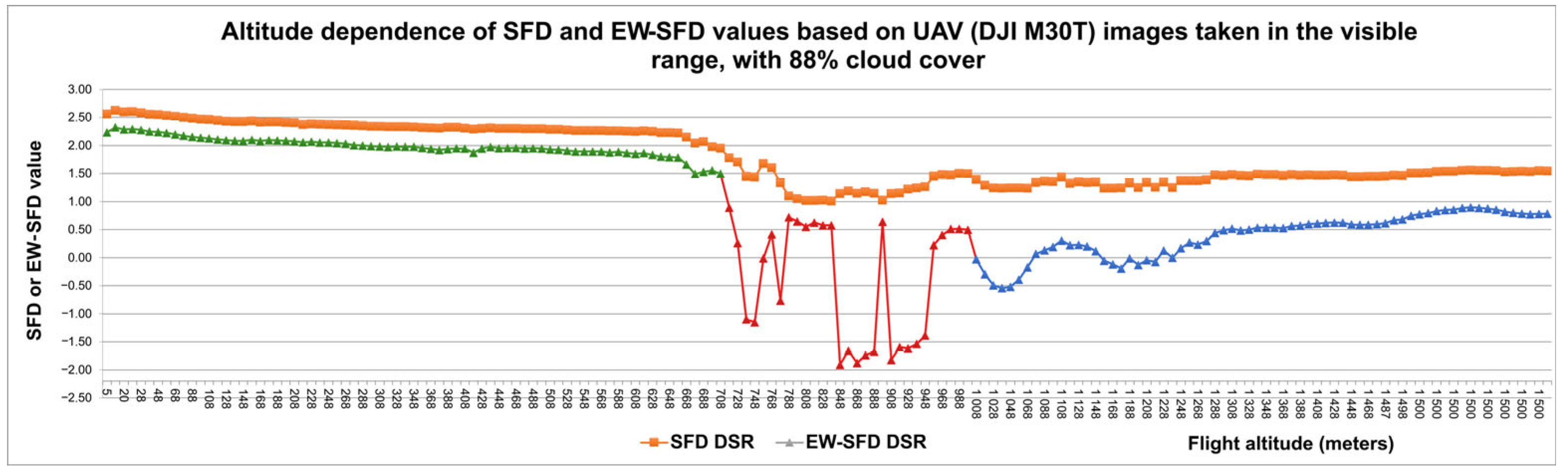
- Below-cloud (5–658 m);
- Transitional (668–788 m);
- Above-cloud (798–1500 m).
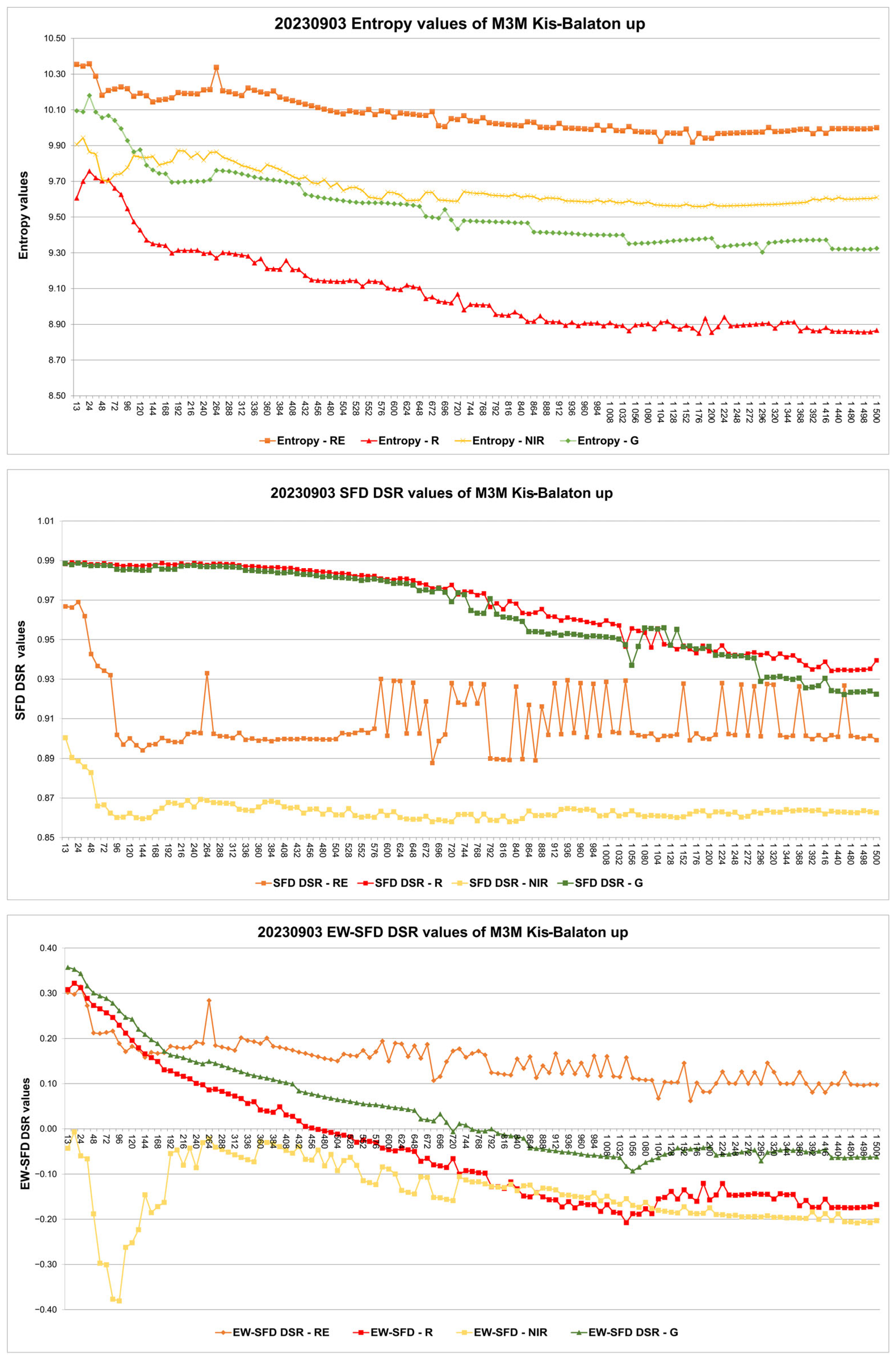
- Below-cloud (5–708 m);
- Transitional (718–1078 m);
- Above-cloud (1088–1500 m).
4. Discussion
5. Conclusions
Funding
Data Availability Statement
Acknowledgments
Conflicts of Interest
Nomenclature
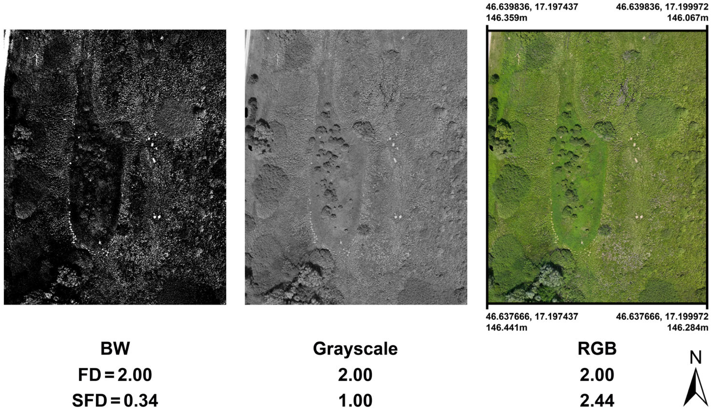
| BW | Black and White (1 bit) |
| CT | Computer Tomography |
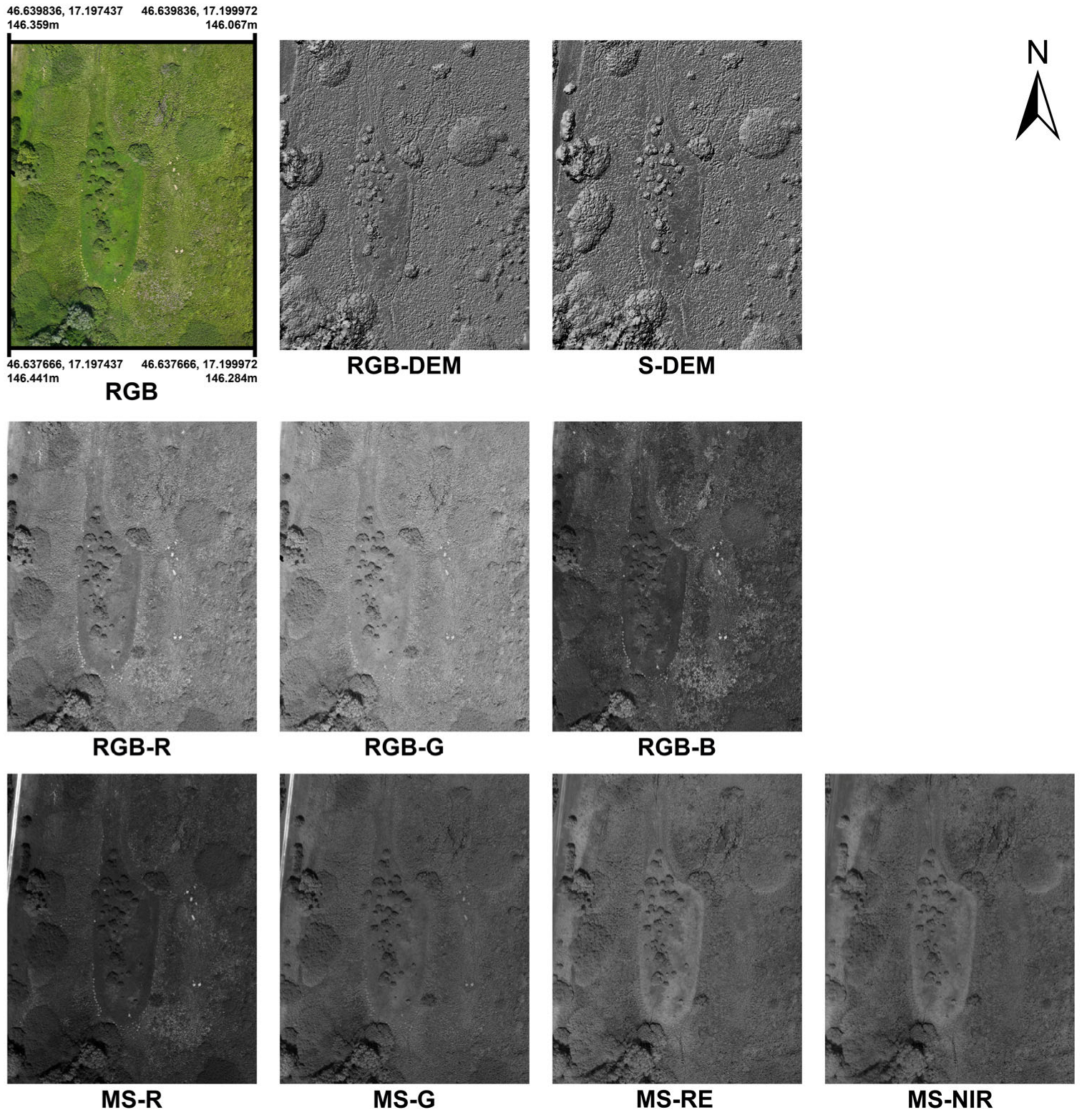
| DEM | Digital Elevation Model |
| EW-SFD | Entropy-Weighted Spectral Fractal Dimension |
| FD | Fractal Dimension |
| FIR | Fared InfraRed |
| GND | Ground (altitude relative to take-off point) |
| H | Entropy |
| MS | Multispectral |
| MS-G | Multispectral camera array G band |
| MS-NIR | Multispectral camera array Near-InfraRed band |
| MS-R | Multispectral camera array R band |
| MS-RE | Multispectral camera array Red-Edge band |
| NIR | Near-InfraRed |
| RE | Red-Edge |
| RGB | Red, Green, Blue (as color-space) |
| RGB-B | B band of RGB image of Bayer sensor |
| RGB-G | G band of RGB image of Bayer sensor |
| RGB-R | R band of RGB image of Bayer sensor |
| SFD | Spectral Fractal Dimension |
| UAV | Unmanned Aerial Vehicle |
| UAS | Unmanned Aerial System |
| VIS | Visible |
References
- Rosenberg, E. Fractal Dimensions of Networks; Springer: Cham, Switzerland, 2020. [Google Scholar]
- Mandelbrot, B.B. Fractals: Forms, Chance and Dimensions; W.H. Freeman and Company: San Francisco, CA, USA, 1977. [Google Scholar]
- Hentschel, H.G.E.; Procaccia, I. The Infinite Number of Generalized Dimensions of Fractals and Strange Attractors. Phys. D 1983, 8, 435–444. [Google Scholar]
- Berke, J. Spectral fractal dimension. In Proceedings of the 7th WSEAS Telecommunications and Informatics (TELE-INFO ’05), Prague, Czech Republic, 12–14 March 2005; pp. 23–26. [Google Scholar]
- Berke, J. Fractal dimension on image processing. In Proceedings of the 4th KEPAF Conference on Image Analysis and Pattern Recognition, Miskolc-Tapolca, Hungary, 28–30 January 2004; Volume 4, p. 20. [Google Scholar]
- Berke, J. The Structure of dimensions: A revolution of dimensions (classical and fractal) in education and science. In Proceedings of the 5th International Conference for History of Science in Science Education, Keszthely, Hungary, 12–16 July 2004. [Google Scholar]
- Berke, J. Real 3D terrain simulation in agriculture. In Proceedings of the 1st Central European International Multimedia and Virtual Reality Conference, Veszprém, Hungary, 6–8 May 2004; Volume 1, pp. 195–201. [Google Scholar]
- Busznyák, J.; Berke, J. Psychovisual comparison of image compression methods under laboratory conditions. In Proceedings of the 4th KEPAF Conference on Image Analysis and Pattern Recognition, Miskolc-Tapolca, Hungary, 28–30 January 2004; Volume 4, pp. 21–28. [Google Scholar]
- Berke, J.; Busznyák, J. Psychovisual Comparison of Image Compressing Methods for Multifunctional Development under Laboratory Circumstances. WSEAS Trans. Commun. 2004, 3, 161–166. [Google Scholar]
- Berke, J. Applied spectral fractal dimension. In Proceedings of the Joint Hungarian-Austrian Conference on Image Processing and Pattern Recognition, Veszprém, Hungary, 11–13 May 2005; pp. 163–170. [Google Scholar]
- Berke, J.; Polgár, Z.; Horváth, Z.; Nagy, T. Developing on exact quality and classification system for plant improvement. J. Univers. Comput. Sci. 2006, 12, 1154–1164. [Google Scholar]
- Berke, J. Measuring of Spectral Fractal Dimension. In Proceedings of the International Conferences on Systems, Computing Sciences and Software Engineering (SCSS 05), Virtual, 10–20 December 2005. Paper No. 62. [Google Scholar]
- Kozma-Bognár, V. The application of Apple systems. J. Appl. Multimed. 2007, 2, 61–70. [Google Scholar]
- Berke, J. Using spectral fractal dimension in image classification. In Innovations and Advances in Computer Sciences and Engineering; Sobh, T., Ed.; Springer: Berlin/Heidelberg, Germany, 2010; pp. 237–242. [Google Scholar]
- Horváth, Z.; Kozma-Bognár, V.; Hegedűs, G.; Berke, J. Fractaltexture test in lawn combination classification with hyperspectral images. In Proceedings of the 12th year of the European conference on Information Systems in Agriculture and Forestry (ISAF), Bled, Slovenia, 27–29 June 2006. [Google Scholar]
- Kozma-Bognar, V.; Berke, J. New Evaluation Techniques of Hyperspectral Data. J. Syst. Cybern. Inform. 2009, 8, 49–53. [Google Scholar]
- Horváth, Z. Separation plant cultures with color mapping. In Proceedings of the 7th International Conference on Computing and Convergence Technology (ICCIT, ICEI and ICACT), ICCCT, Seoul, Republic of Korea, 3–5 December 2012; pp. 363–366. [Google Scholar]
- Berke, J.; Bíró, T.; Burai, P.; Kováts, L.D.; Kozma-Bognar, V.; Nagy, T.; Tomor, T.; Németh, T. Application of remote sensing in the red mud environmental disaster in Hungary. Carpathian J. Earth Environ. Sci. 2013, 8, 49–54. [Google Scholar]
- Bíró, T.; Tomor, T.; Lénárt, C.S.; Burai, P.; Berke, J. Application of remote sensing in the red sludge environmental disaster in Hungary. Acta Phytopathol. Entomol. Hung. 2012, 47, 223–231. [Google Scholar]
- Burai, P.; Smailbegovic, A.; Lénárt, C.; Berke, J.; Milics, G.; Tomor, T.; Bíró, T. Preliminary Analysis of Red Mud Spill Based on Ariel Imagery. Acta Geogr. Debrecina Landsc. Environ. 2011, 5, 47–57. [Google Scholar]
- Berke, J.; Kozma-Bognár, V. Investigation possibilities of turbulent flows based on geometric and spectral structural properties of aerial images. In Proceedings of the 10th National Conference of the Hungarian Society of Image Processing and Pattern Recognition, Kecskemét, Hungary, 27–30 January 2015; pp. 295–304. [Google Scholar]
- Kozma-Bognár, V.; Berke, J. Entropy and fractal structure based analysis in impact assessment of black carbon pollutions. Georg. Agric. 2013, 17, 53–68. [Google Scholar]
- Kozma-Bognar, V.; Berke, J. Determination of optimal hyper- and multispectral image channels by spectral fractal structure. In Innovations and Advances in Computing, Informatics, Systems Sciences, Networking, and Engineering; Lecture Notes in Electrical Engineering (LNEE); Sobh, T., Elleithy, K., Eds.; Springer International Publishing: Cham, Switzerland, 2015; Volume 313, pp. 255–262. [Google Scholar]
- Chamorro-Posada, P. A simple method for estimating the fractal dimension from digital images: The compression dimension. Chaos Solitions Fractals 2016, 91, 562–572. [Google Scholar]
- Karydas, C.G. Unified scale theorem: A mathematical formulation of scale in the frame of Earth observation image classification. Fractal Fract. 2021, 5, 127. [Google Scholar] [CrossRef]
- Dachraoui, C.; Mouelhi, A.; Drissi, C.; Labidi, S. Chaos theory for prognostic purposes in multiple sclerosis. Trans. Inst. Meas. Control. 2021, 0, 1–12. [Google Scholar] [CrossRef]
- Abdul-Adheem, W. Image Processing Techniques for COVID-19 Detection in Chest CT. J. Al-Rafidain Univ. Coll. Sci. 2022, 52, 218–226. [Google Scholar]
- Frantík, P. An Approach for Accurate Measurement of Fractal Dimension Distribution on Fracture Surfaces. Trans. VSB–Tech. Univ. Ostrav. Civ. Eng. Ser. 2022, 22, 7–12. [Google Scholar]
- Csákvári, E.; Halassy, M.; Enyedi, A.; Gyulai, F.; Berke, J. Is Einkorn Wheat (Triticum monococcum L.) a Better Choice than Winter Wheat (Triticum aestivum L.)? Wheat Quality Estimation for Sustainable Agriculture Using Vision-Based Digital Image Analysis. Sustainability 2021, 13, 12005. [Google Scholar] [CrossRef]
- Kevi, A.; Berke, J.; Kozma-Bognár, V. Comparative analysis and methodological application of image classification algorithms in higher education. J. Appl. Multimed. 2023, XVIII/1, 13–16. [Google Scholar]
- Vastag, V.K.; Óbermayer, T.; Enyedi, A.; Berke, J. Comparative study of Bayer-based imaging algorithms with student participation. J. Appl. Multimed. 2019, XIV/1, 7–12. [Google Scholar] [CrossRef]
- Berke, J.; Kozma-Bognár, V. Measurement and comparative analysis of gain noise on data from Bayer sensors of unmanned aerial vehicle systems. In X. Hungarian Computer Graphics and Geometry Conference; SZTAKI: Budapest, Hungary, 2022; pp. 136–142. [Google Scholar]
- Shannon, C.E. A mathematical theory of communication. Bell Syst. Tech. J. 1948, 27, 379–423. [Google Scholar] [CrossRef]
- Shannon, C.E. Prediction and entropy of printed English. Bell Syst. Tech. J. 1951, 30, 50–64. [Google Scholar] [CrossRef]
- Berke, J.; Gulyás, I.; Bognár, Z.; Berke, D.; Enyedi, A.; Kozma-Bognár, V.; Mauchart, P.; Nagy, B.; Várnagy, Á.; Kovács, K.; et al. Unique algorithm for the evaluation of embryo photon emission and viability. Sci. Rep. 2024, 14, 15066. [Google Scholar] [CrossRef]
- Bodis, J.; Nagy, B.; Bognar, Z.; Csabai, T.; Berke, J.; Gulyas, I.; Mauchart, P.; Tinneberg, H.R.; Farkas, B.; Varnagy, A.; et al. Detection of Ultra-Weak Photon Emissions from Mouse Embryos with Implications for Assisted Reproduction. J. Health Care Commun. 2024, 9, 9041. [Google Scholar]
- Biró, L.; Kozma-Bognár, V.; Berke, J. Comparison of RGB Indices used for Vegetation Studies based on Structured Similarity Index (SSIM). J. Plant Sci. Phytopathol. 2024, 8, 7–12. [Google Scholar]
- Kozma-Bognár, K.; Berke, J.; Anda, A.; Kozma-Bognár, V. Vegetation mapping based on visual data. J. Cent. Eur. Agric. 2024, 25, 807–818. [Google Scholar]
- Berzéki, M.; Kozma-Bognár, V.; Berke, J. Examination of vegetation indices based on multitemporal drone images. Gradus 2023, 10, 1–6. [Google Scholar]
- Mandelbrot, B.B. The Fractal Geometry of Nature; W.H. Freeman and Company: New York, NY, USA, 1983; p. 15. [Google Scholar]
- Barnsley, M.F. Fractals Everywhere; Academic Press: Cambridge, MA, USA, 1998; pp. 182–183. [Google Scholar]
- Voss, R. Random fractals: Characterisation and measurement. In Scaling Phenomena in Disordered Systems; Pynn, R., Skjeltorps, A., Eds.; Plenum: New York, NY, USA, 1985. [Google Scholar]
- Peleg, S.; Naor, J.; Hartley, R.; Avnir, D. Multiple Resolution Texture Analysis and Classification. IEEE Trans. Pattern Anal. Mach. Intell. 1984, 4, 518–523. [Google Scholar] [CrossRef]
- Turner, M.T.; Blackledge, J.M.; Andrews, P.R. Fractal Geometry in Digital Imaging; Academic Press: Cambridge, MA, USA, 1998; pp. 45–46, 113–119. [Google Scholar]
- Goodchild, M. Fractals and the accuracy of geographical measure. Math. Geol. 1980, 12, 85–98. [Google Scholar]
- DeCola, L. Fractal analysis of a classified Landsat scene. Photogramm. Eng. Remote Sens. 1989, 55, 601–610. [Google Scholar]
- Clarke, K. Scale based simulation of topographic relief. Am. Cartogr. 1988, 12, 85–98. [Google Scholar]
- Shelberg, M. The Development of a Curve and Surface Algorithm to Measure Fractal Dimension. Master’s Thesis, Ohio State University, Columbus, OH, USA, 1982. [Google Scholar]
- Berke, J. Measuring of spectral fractal dimension. New Math. Nat. Comput. 2007, 3, 409–418. [Google Scholar]
- Fréchet, M.M. Sur quelques points du calcul fonctionnel. Rend. Circ. Matem. 1906, 22, 1–72. [Google Scholar] [CrossRef]
- Baire, R. Sur les fonctions de variables réelles. Ann. Mat. 1899, 3, 1–123. [Google Scholar]
- Serra, J.C. Image Analysis and Mathematical Morphology; Academic Press: London, UK, 1982. [Google Scholar]
- Mie, G. Beiträge zur Optik trüber Medien, speziell kolloidaler Metallösungen. Ann. Phys. 1908, 25, 377–445. [Google Scholar]
- Sabins, F.F. Remote Sensing. In Principles and Interpretation; W.H. Freeman and Company: Los Angeles, CA, USA, 1987. [Google Scholar]


| Methods | Main Facts |
|---|---|
| Box Counting [42] | most popular, can be easily algorithmized in the case of images |
| Epsilon-Blanket [43] | to curve |
| Fractional Brownian Motion [44] | similar box counting |
| Power Spectrum [44] | digital fractal signals |
| Hybrid Methods [45] | calculate the fractal dimension of 2D using 1D methods |
| Perimeter–Area relationship [46] | to classify different type images |
| Prism Counting [47] | for a one-dimensional signal |
| Walking-Divider [48] | practical to length |
| Band Name | Sensor Name (Center Wavelength (nm), Bandwidth (nm)) | |||||
|---|---|---|---|---|---|---|
| MicaSense Dual | MicaSense Altum-PT | Sentera 6x Multispectral | Parrot Sequoia+ Multispectral | DJI P4 Multispectral | DJI M3 Multispectral | |
| Coastal Blue | 444 ± 28 | - | - | - | 450 ± 16 | - |
| Blue | 475 ± 32 | 475 ± 32 | 475 ± 30 | - | - | - |
| Green | 531 ± 14 | - | - | - | - | - |
| Green | 560 ± 27 | 560 ± 27 | 550 ± 20 | 550 ± 40 | 560 ± 16 | 560 ± 16 |
| Red | 650 ± 16 | - | - | - | 650 ± 16 | 650 ± 16 |
| Red | 668 ± 14 | 668 ± 14 | 670 ± 30 | 660 ± 40 | - | - |
| Red Edge | 705 ± 10 | - | - | - | - | - |
| Red Edge | 717 ± 12 | 717 ± 12 | 715 ± 10 | - | - | - |
| Red Edge | 740 ± 18 | - | - | 735 ± 10 | 730 ± 16 | 730 ± 16 |
| Near Infrared | 842 ± 57 | 842 ± 57 | 840 ± 30 | 790 ± 40 | 860 ± 26 | 860 ± 26 |
| LWIR | - | 10.5 ± 6 μm | - | - | - | - |
| Image | n | S (Bit) | SFDmeasured | Entropy |
|---|---|---|---|---|
| RGB | 3 | 8 | 2.4592 | 18.1197 |
| MS | 4 | 16 | 2.3465 | 22.0394 |
| RGB-DEM | 1 | 8 | 0.9883 | 7.5330 |
| MS-DEM | 1 | 16 | 0.9962 | 14.1626 |
| RGB-R | 1 | 8 | 1.0000 | 7.3043 |
| RGB-G | 1 | 8 | 1.0000 | 7.2245 |
| RGB-B | 1 | 8 | 1.0000 | 7.1399 |
| MS-R | 1 | 16 | 0.9976 | 12.7551 |
| MS-G | 1 | 16 | 0.9963 | 13.1113 |
| MS-RE | 1 | 16 | 0.9746 | 13.3359 |
| MS-NIR | 1 | 16 | 0.9637 | 13.0143 |
| ALL | 9 | 16 | 4.1281 | 22.0394 |
| RGB-DEM | RGB-R | RGB-G | RGB-B | Maximum Values | |
|---|---|---|---|---|---|
| SFD values measured without boundary conditions | 0.9883 | 1 | 1 | 1 | 1 |
| SFD values measured based on 10 m height—as boundary condition | 0.9996 | 0.9996 | 0.9996 | ||
| Entropy values measured without boundary conditions | 7.5330 | 7.3043 | 7.2245 | 7.1399 | 8 |
| Entropy values measured based on 10 m height—as boundary condition | 4.3499 | 4.3061 | 4.2527 |
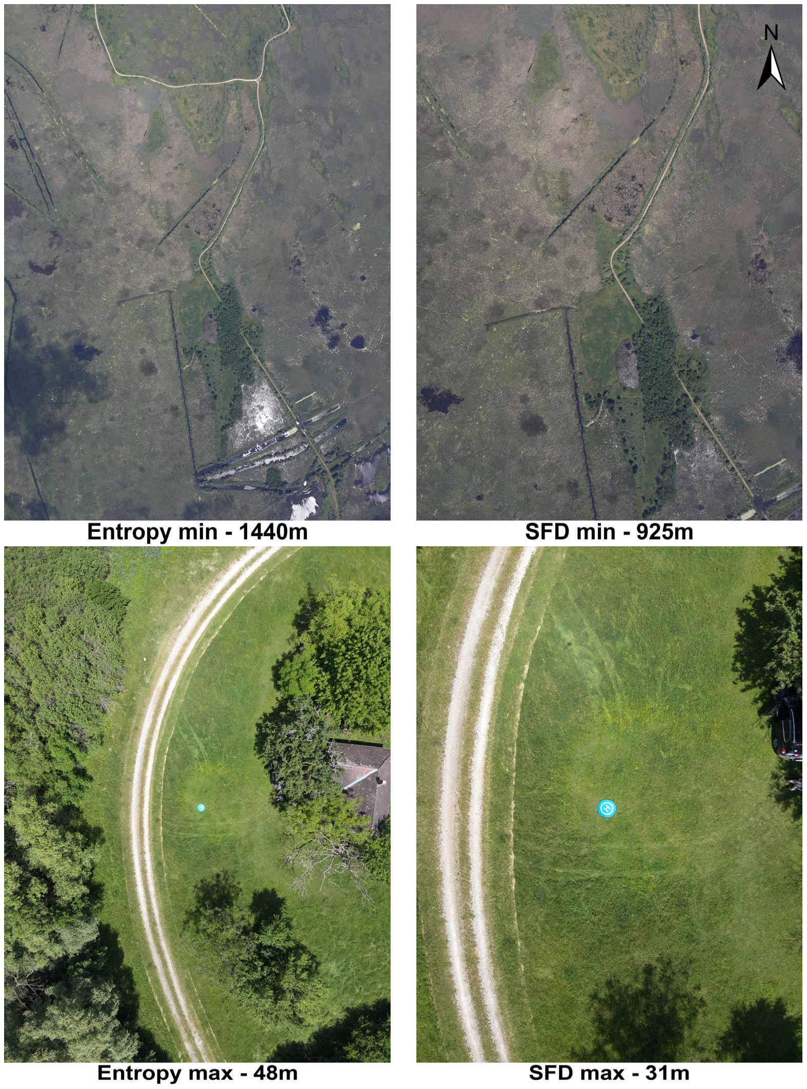
| Hmax | Hmin | SFDmax | SFDmin | EW-SFDmax | EW-SFDmin | |
|---|---|---|---|---|---|---|
| Numerical values | 15.70 | 12.88 | 2.58 | 2.21 | 2.30 | 1.67 |
| Ascent height (m) | 48 | 1440 | 28 | 920 | 28 | 976 |
| Numerical values | 15.71 | 12.97 | 2.57 | 2.20 | 2.29 | 2.02 |
| Descent height (m) | 56 | 1072 | 31 | 925 | 31 | 1295 |
| H average | Hstdev | SFD average | SFDstdev | EW-SFD average | EW-SFD stdev | |
|---|---|---|---|---|---|---|
| Visible A | 14.47 | 0.54 | 2.37 | 0.10 | 2.02 | 0.13 |
| Visible B | 10.14 | 1.09 | 1.71 | 0.32 | 0.54 | 1.04 |
| Visible C | 8.63 | 0.37 | 1.37 | 0.15 | 0.18 | 0.75 |
| FIR A | 14.06 | 0.65 | 2.56 | 0.04 | 2.32 | 0.06 |
| FIR B | 11.59 | 1.16 | 2.45 | 0.05 | 2.10 | 0.10 |
| FIR C | 6.95 | 0.37 | 1.56 | 0.22 | 0.91 | 0.26 |
| H average | Hstdev | SFD average | SFDstdev | EW-SFD average | EW-SFD stdev | |
|---|---|---|---|---|---|---|
| FIR I | 13.97 | 0.71 | 2.56 | 0.04 | 2.31 | 0.06 |
| FIR II | 7.96 | 0.76 | 1.78 | 0.05 | 1.21 | 0.08 |
| FIR III | 6.85 | 0.11 | 1.54 | 0.19 | 0.88 | 0.20 |
| FIR A | 14.06 | 0.65 | 2.56 | 0.04 | 2.32 | 0.06 |
| FIR B | 11.59 | 1.16 | 2.45 | 0.05 | 2.10 | 0.10 |
| FIR C | 6.95 | 0.37 | 1.56 | 0.22 | 0.91 | 0.26 |
| Hmax | Hmin | SFDmax | SFDmin | EW-SFDmax | EW-SFDmin | |
|---|---|---|---|---|---|---|
| Red | 9.76 | 8.85 | 0.99 | 0.93 | 0.32 | −0.21 |
| R-altitude | 24 | 1176 | 14 | 1428 | 14 | 1044 |
| Green | 10.18 | 9.30 | 0.99 | 0.92 | 0.36 | −0.09 |
| G-altitude | 24 | 1296 | 24 | 1452 | 13 | 1056 |
| Red Edge | 10.35 | 9.92 | 0.97 | 0.89 | 0.31 | 0.06 |
| altitude | 24 | 1164 | 24 | 684 | 24 | 1164 |
| Near | 9.94 | 9.56 | 0.90 | 0.86 | −0.01 | −0.38 |
| Infrared alt. | 14 | 1176 | 14 | 720 | 14 | 96 |
| All layers together | 22.2646 | 22.2633 | 2.8364 | 2.6248 | 2.4206 | 1.9846 |
| 84–96 | 12 | 36 | 1368 | 14–24 | 1368 |
Disclaimer/Publisher’s Note: The statements, opinions and data contained in all publications are solely those of the individual author(s) and contributor(s) and not of MDPI and/or the editor(s). MDPI and/or the editor(s) disclaim responsibility for any injury to people or property resulting from any ideas, methods, instructions or products referred to in the content. |
© 2025 by the author. Licensee MDPI, Basel, Switzerland. This article is an open access article distributed under the terms and conditions of the Creative Commons Attribution (CC BY) license (https://creativecommons.org/licenses/by/4.0/).
Share and Cite
Berke, J. Application Possibilities of Orthophoto Data Based on Spectral Fractal Structure Containing Boundary Conditions. Remote Sens. 2025, 17, 1249. https://doi.org/10.3390/rs17071249
Berke J. Application Possibilities of Orthophoto Data Based on Spectral Fractal Structure Containing Boundary Conditions. Remote Sensing. 2025; 17(7):1249. https://doi.org/10.3390/rs17071249
Chicago/Turabian StyleBerke, József. 2025. "Application Possibilities of Orthophoto Data Based on Spectral Fractal Structure Containing Boundary Conditions" Remote Sensing 17, no. 7: 1249. https://doi.org/10.3390/rs17071249
APA StyleBerke, J. (2025). Application Possibilities of Orthophoto Data Based on Spectral Fractal Structure Containing Boundary Conditions. Remote Sensing, 17(7), 1249. https://doi.org/10.3390/rs17071249