Abstract
The study of secondary craters on the Moon is vital for understanding lunar impact dynamics and surface evolution. However, this task is complicated by sample imbalance, with primary crater samples outnumbering those of secondary craters, and by the reliance on time-intensive manual methods or limited automated techniques. While many previous studies have focused on the manual or automated differentiation of secondary craters, few have addressed the interpretation of variables and models. In this study, we propose a machine-learning-based approach using the CatBoost algorithm to classify craters based on variables extracted from Digital Elevation Model (DEM) data. These variables include those from previous research as well as new ones introduced here, such as slope and density with Gaussian summation. Despite data imbalance and noise, the model achieves a classification accuracy of 0.8788, with a precision of 0.7922, a recall rate of 0.7412, and an F1 score of 0.7658 for secondary craters. To enhance interpretations, Shapley additive explanations (SHAP) and partial dependence plots (PDPs) are applied to evaluate variable importance and visualize the marginal effects of key variables, indicating the density variables playing a key role in crater classification.
1. Introduction
Craters are among the most extensively studied geomorphological landforms in planetary science, containing a wealth of geological history. Their significance is evident in various applications, including determining numerical ages [,], analyzing impact distributions, and reconstructing impact histories. Traditionally, these applications assume that all craters are primary craters formed directly by the impact of asteroids or comets. However, ejecta deposits produced by primary impact events could form craters (i.e., secondaries) e.g., [,]. Some of them have similar morphology to primary craters of the same size [,].
Secondary craters comprise a substantial portion of small craters and often introduce uncertainties in the crater size–frequency distribution (CSFD) [,,,]. Therefore, accurately distinguishing between primary and secondary craters is essential for enhancing the reliability of crater-based age estimates. Furthermore, this differentiation is vital for impact distribution studies and provides insights into the characteristics of the original impact events.
Despite efforts to differentiate primary and secondary craters, many existing methods rely heavily on manual identification. Various studies have employed different approaches, such as excluding secondary craters based on their morphological characteristics [,,,,,,], multispectral imaging to analyze the iron content on crater surfaces [], assessing crater degradation [,], and conducting visual inspections []. Although these methods yield accurate results, they are time-consuming and require specialized expertise, making them challenging to apply to large areas efficiently.
Distinguishing primary and secondary craters is difficult because of a severe sample imbalance, as secondary craters are significantly underrepresented in datasets compared to primary craters. The number of available primary crater samples can be several times greater than that of secondary crater samples.This imbalance challenges machine learning models, which often become biased due to the dominance of primary craters in training data, leading to reduced accuracy in identifying the typically smaller and irregularly shaped secondary craters. To tackle this issue, this study extracts a comprehensive range of variables from Digital Elevation Model (DEM) data. Alongside variables from previous research, new variables are introduced, such as slope and density with Gaussian Summation, to enhance the model’s ability to differentiate between crater types.
While some automated methods have been developed, many are rule-based approaches that focus on spatial crater distribution. Techniques utilizing Monte Carlo simulations and clustering algorithms [,], as well as Voronoi polygons for non-random distributions [], have shown promise. However, these methods are limited by the relatively small number of variables they use, and the performance of the automated algorithms employed is weaker compared to machine learning algorithms. As a result, they struggle to effectively capture the distinction between primary and secondary craters.
In recent years, machine learning and deep learning methods have been introduced into lunar research, particularly for crater recognition and remote sensing data classification. Yamamoto et al. proposed a fully automated algorithm using rotational pixel swapping for crater detection []. Benedix et al. used YOLO v3, trained on Thermal Emission Imaging System data, for automated detection []. Wang et al. applied machine learning to detect craters from DEMs and extract 3D morphometric data []. Lin et al. presented an end-to-end deep learning pipeline using CNNs for lunar craters smaller than 50 km []. Lagain et al. used a CNN-based algorithm for small-impact craters on Mars imagery, using cluster analysis to filter secondary craters []. Fairweather et al. adapted YOLO v3 for Lunar Reconnaissance Orbiter NAC images [], while Latorre et al. applied transfer learning with a U-Net model, refined with Ceres images, using data augmentation and post-processing for crater detection []. These approaches offer a significant advantage over rule-based methods, as they can learn optimal variables from large training datasets, thus better capturing the complexities of crater structures and improving the distinction between primary and secondary craters. However, the intricate “black-box” nature of these models poses challenges in interpreting their outputs [].
To address this issue, Lundberg and Lee [] proposed the Shapley additive explanations (SHAP) method, which provides a robust framework for interpreting model predictions and evaluating variable importance. The growing adoption of SHAP in various studies [] underscores its potential to enhance understanding in this field. Complementary to SHAP, the partial dependence plot (PDP), introduced by [], visualizes the marginal effect of an individual variable on model predictions. To construct a PDP, we first select a variable of interest, substitute its different values into the PDP function, use the black-box model to make predictions, and calculate the average of the predicted probability. Finally, we plot the relationship between the variable values and the predicted probability, which forms the partial dependence plot. This method is useful in revealing the non-linear relationships and complex interactions in the context of crater classification.
This paper presents a machine-learning-based approach for distinguishing between primary and secondary craters through an analysis of crater characteristics. By leveraging SHAP analysis, we assessed the importance of various variables extracted from Digital Elevation Model (DEM) images in crater classification. Additionally, PDP was employed to visualize the influence of specific variables on the classification outcomes, providing further insight into the model’s behavior. Our method not only integrates variable extraction techniques from previous studies [] but also introduces new variables, thereby advancing the current state of crater analysis and contributing to more accurate geological assessments.
2. Materials and Methods
The workflow for crater classification is presented in Figure 1. In this study, crater data from Robbins 2018 [] and Singer 2020 [], along with a Digital Elevation Model (DEM) [], served as the foundational dataset for analysis. Key variables and indices—namely crater density, depth-to-diameter ratio, Voronoi metrics, and slope—were systematically extracted to capture the discriminative characteristics essential for classification. The dataset was subsequently partitioned into training and test sets, with the classifier model trained on the former to enable accurate differentiation of crater types. Model performance was rigorously evaluated on the test set, with accuracy metrics employed to ensure robustness and general applicability. Lastly, variable importance was examined using Shapley additive explanations (SHAP) and partial dependence plot (PDP) methodologies, providing insights into the contribution of each variable to the model’s classification decisions.
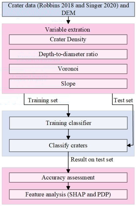
Figure 1.
Workflow of crater classification using variable extraction, machine learning model training, and variable analysis [,].
2.1. Data Preparation
High resolution and precise topographic representation are critical for identifying and analyzing the detailed variables of craters. In this study, we primarily utilized the Digital Elevation Model (DEM) data (SLDEM) [] provided by the Lunar Reconnaissance Orbiter (LRO)’s Lunar Orbiter Laser Altimeter (LOLA) and Kaguya (SELENE)’s Terrain Camera (TC). These data, released by the LOLA and SELENE teams, offer near-global coverage of the lunar topography with resolutions of 512 pixels/degree and 59 meters/pixel, spanning latitudes from −60° to +60° with complete longitudinal coverage. From SLDEM data, we were able to extract detailed terrain information for the target regions.
Additionally, to strengthen the foundation of this research, we referenced the Robbins Lunar Crater Database compiled by Stuart J. Robbins in 2018 []. This database provides exhaustive information on all known lunar craters, including the central coordinates, diameters, depths, and rim characteristics of craters. These detailed parameters cover craters ranging in diameter from 1 kilometer to several hundred kilometers, offering a rich source of training data for this study, facilitating model validation and performance evaluation.
Of particular note, this study employed secondary crater annotation data provided by Singer [], specifically for the Copernicus Crater region (38.392578°N to 10.044922°S, 39.898437°W to 8.648437°W) and the Kepler Crater region (16.439453°N to 0.748047°S, 53.455078°W to 31.580078°W). These annotations served as valuable references for our model, enabling a more accurate distinction between primary and secondary craters, thereby enhancing the accuracy of automated detection and classification. To ensure consistent spatial alignment, all coordinate data from the Singer 2020 [] and Robbins 2018 [] datasets were converted to the same cylindrical projection system used by SLDEM2015.
In contrast to the other four regions in Singer 2020 [] (Orientale, unnamed in SPA, unnamed near Orientale, and unnamed in Procellarum), the Kepler and Copernicus regions are of moderate size and contain a relatively larger number of annotations. Most of the annotated craters in these two regions are large enough in diameter for the 59 m/pixel resolution of the SLDEM to adequately capture the topographic variations associated with crater morphology. In comparison, and in particular, the Orientale region is characterized by a sparse distribution of secondary craters; the number of secondary crater annotations in Singer 2020 [] is substantially lower than that in Robbins 2018 [] (fewer than 300 annotations compared to over 100,000 craters in total), and these secondary craters are widely separated from each other. This sparse distribution, defined by both the limited number of annotations and the large spatial distances between them, combined with the high density of crater samples from Robbins 2018 [], significantly complicates the resolution of the sample imbalance problem. As a result, minimal differences emerge in the computed density-based variables between primary and secondary craters, hindering the model’s ability to effectively distinguish between the two classes. For these reasons, we did not select the Orientale region as a study area.
Because there is overlap between the crater annotations in the Robbins Lunar Crater Database and the Singe r2020 [] dataset within the target regions, we calculated the Intersection over Union (IoU) values between the overlapping crater annotations from the two databases. When IoU ≥ 0.5, the corresponding crater annotations from the Robbins database were removed.
However, it is important to note that Singer’s article states that not all secondary craters in their study area were digitized—only the most confidently identified candidates were included. This limitation may introduce potential biases, as some secondary craters could have been misclassified as primary craters.
To address this, we implemented a five-fold cross-validation-based approach. Specifically, we randomly divided the dataset into five equal parts.The model was then trained five times, each time with a different fold serving as the test set while the remaining four folds were used for training. After each training step, we used the model to predict the test set. If any sample originally labeled as a primary crater had a confidence score for secondary craters (class 1) greater than 0.8, we relabeled that sample as a secondary crater.
The final model performance was evaluated using the updated dataset, which incorporated the corrected labels. The statistical data of the various types of craters in different regions are shown in Table 1.

Table 1.
Statistical data of craters in research area.
2.2. Variable Extraction
Different craters exhibit distinct characteristics, which are crucial for classifying secondary craters. In the process of extracting crater variables from DEM data, we selected several variables closely related to crater morphology and structure. The primary variables and indices included crater density, depth-to-diameter ratio, Voronoi metrics, and slope.
The choice of variables was influenced by the constraints of the available datasets. Specifically, we utilized the SLDEM, Robbins 2018 [], and Singer 2020 [] datasets. While both Robbins 2018 [] and Singer 2020 [] provide detailed crater annotations, Robbins 2018 [] offers additional shape descriptors such as eccentricity, which are useful for variable extraction. In contrast, the Singer 2020 [] dataset contains only the latitude (Lat_deg) and longitude (Lon_deg) of the crater center as well as its diameter (Diam_km), without further morphological details. This restricted our ability to extract and apply other potential variables that rely on more-detailed shape descriptors.
2.2.1. Crater Density
Inspired by previous work [], we divided the crater density variable into cluster density and chain density to more accurately reflect the distribution characteristics of different types of craters.
Cluster density is defined as the number of craters within a radius n times the radius of a central crater, where these craters have radii similar to the central crater (within a 20% radius difference). This variable measures the degree of clustering in a localized area, helping to identify densely distributed groups of secondary craters [].
We further applied Gaussian summation to the calculation of cluster density to more accurately account for the influence of each crater on the central crater. The Gaussian-weighted method ensures that craters closer to the central crater contribute more to the cluster density, while those further away contribute less, providing a more realistic reflection of the spatial distribution and clustering of secondary craters. The specific method is as follows:
- Define the central region: For each central crater, define a circular region centered on the crater, with a radius n times the crater’s radius. The value of n ranges from 10 to 100, with a step size of 10.
- Filter craters with similar radii: within this circular region, identify all craters whose radii are similar to that of the central crater (within a 20% radius difference).
- Calculate Gaussian summation: compute the Gaussian-weighted value for each crater relative to the central crater and sum these values to obtain the cluster density. The formula for the Gaussian summation is as follows (Equation (1)):
To analyze the cluster density within different ranges, we selected multiple values (10, 20, 30, 40, 50, 60, 70, 80, 90, 100) and a parameter (2, 4, 6, 8, 10) as well as computed the density values within each range. This approach allowed us to capture density information across different scales, providing a more comprehensive understanding of crater distribution characteristics.
By using this multi-scale analysis, we can better assess the clustering behavior of craters and identify potential secondary crater patterns at varying distances from the central crater. This enables a deeper insight into the spatial organization of craters and their classification.
Chain density is defined by calculating the number of craters with similar radii (same as cluster density, within a 20% radius difference) to the central crater, located within a rectangular region along a specific direction, with rotations in 30-degree intervals. This variable captures the distribution characteristics of crater chains, particularly useful for identifying linear patterns formed by secondary impacts on planetary surfaces.
The specific calculation steps are as follows:
- Define the rectangular region: starting from the center of the central crater, define a rectangular region along specific directions (0°, 30°, 60°, 90°, 120°, 150°). The width of the region is 40 times the radius of the central crater, and the length is 100 times the radius.
- Filter craters with similar radii: within this rectangular region, identify all craters with radii similar to that of the central crater.
- Calculate Gaussian summation: similar to cluster density, apply Gaussian weighting to the craters in each direction to compute the chain density. The formula for chain density is as follows (Equation (3)):
We employed the same Gaussian function used for cluster density, with values set to (10, 20, 30, 40, 50, 60, 70, 80, 90, 100) and a values set to (3, 6, 9, 12, 15), to perform the weighting. This consistent approach more effectively captured the spatial distribution characteristics of chain-like structures.
The application of Gaussian summation to these enhanced density variables not only effectively describes the clustering and chain distribution of craters but also improves the classification and detection performance of the model. These improvements provide a more accurate representation of the spatial patterns of craters, enhancing the overall ability of the model to distinguish between primary and secondary craters.
2.2.2. Depth-to-Diameter Ratio
The depth-to-diameter ratio (depth_diam_rat) is an important index that describes crater morphology, reflecting the relationship between a crater’s depth and diameter. This ratio can reveal morphological differences among various types of craters. For instance, primary impact craters typically exhibit a high depth-to-diameter ratio, whereas secondary craters formed by debris impacts generally have a low ratio. In this study, we extracted the depth and diameter of each crater using Digital Elevation Model (DEM) data, and, based on these, we calculated the depth-to-diameter ratio according to Equation (4):
where depth_diam_rat is the depth-to-diameter ratio, D represents the diameter of the crater, represents the average of all elevation data in the crater area, and is the depth of the impact crater.
2.2.3. Voronoi Diagram
The Voronoi diagram, as a spatial partitioning method, divides a space into regions where each point within a region is closer to a specific generating point (or seed point) than to any other generating point. This approach has significant applications in crater classification, as it effectively analyzes the spatial relationships and distribution patterns among craters. In this study, a Voronoi diagram was used to characterize the influence range of each crater, providing a precise basis for variable extraction.
By generating a Voronoi diagram based on the coordinates of crater centers, each Voronoi cell represents the area of influence of the corresponding crater. The size of the Voronoi cell is used to infer the spatial density of crater distributions and their mutual influences. For instance, compact Voronoi cells typically indicate high crater density, while large cells suggest more isolated craters.
In this study, we extracted the area of the Voronoi cells as the primary Voronoi variable. A schematic diagram of the Voronoi variables is shown in Figure 2, where orange numbers represent the area of each Voronoi cell, and yellow lines indicate the cell boundaries.
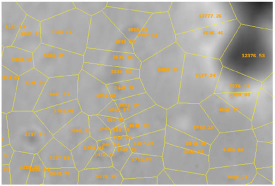
Figure 2.
A schematic representation of the Voronoi variable associated with the Copernicus crater. The diagram illustrates the spatial subdivision of the crater region into Voronoi cells based on point distributions. The orange numerical labels indicate the area of each Voronoi cell, while the yellow lines represent the boundaries separating adjacent cells.
2.2.4. Slope
In Geographic Information Systems (GISs), slope typically refers to the steepness or gradient of a surface, representing the inclination of the terrain. The calculation of slope involves elevation data, and it can be estimated by measuring changes in elevation using Digital Elevation Models (DEMs). Slope is generally expressed either as a percentage or in degrees. Percentage slope represents the ratio of elevation change to horizontal distance, while slope degree is expressed as an angular measurement.
This paper employed two slope-related variables, namely, the average slope and the slope angle.
The slope angle was defined as the angle between the radius and the hypotenuse of a right triangle formed by the crater’s depth and radius. Because the slope angle is typically small, this study used its complementary angle, , to represent the overall slope characteristics of the crater. A large complementary angle corresponds to a gentle overall slope, while a small complementary angle indicates a steep slope. The use of the complementary angle allows for a more comprehensive characterization of the crater’s morphology, offering a more intuitive and comparable metric, particularly useful when dealing with small slope angles. The complementary angle is calculated according to Equation (5):
where is the slope angle, D represents the diameter of the crater, and d represents the depth of the crater.
The slope S was determined by calculating the first-order partial derivatives of the elevation z with respect to the x and y directions for each pixel in the DEM. These derivatives represent the rate of change in elevation in each direction. The formula for calculating slope is as follows (Equation (6)):
where z represents the elevation value, and and are the rates of elevation change in the X and Y directions, respectively, i.e., the slope components. From these components, the total slope S at each point can be calculated, which is defined by Equation (7):
The depth-to-diameter ratio is a key parameter in crater variable analysis. However, relying solely on the depth-to-diameter ratio without considering the average slope when classifying secondary craters may lead to incorrect classification, as varying average slope values around a crater can affect the measurement of the depth-to-diameter ratio. Therefore, to achieve a more precise analysis of crater characteristics, we introduced the average slope variable by calculating the arithmetic mean of the slope values for all pixel points within a given area (Equation (8)):
where is the average slope, represents the slope value at the i-th pixel, and N is the total number of pixels in the region of interest.
The method for calculating the average slope is illustrated in Figure 3. For each crater, two square regions are defined, centered at the crater’s center. One square has a side length equal to 1.2 times the crater’s diameter (small square), and the other has a side length equal to 2.0 times the crater’s diameter (large square). These two regions, referred to as the small and large squares, are used to capture the slope variations in the crater and its surrounding area.
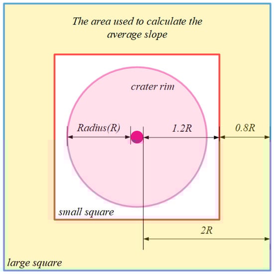
Figure 3.
The method for calculating the average slope. The blue square represents the large square, while the red square indicates the small square. The magenta circle symbolizes the crater rim, and the yellow area highlights the region used to calculate the average slope.
To calculate the difference in slope values between the two regions, we subtract the total slope value within the small square from the total slope value within the large square. The difference in the area of the two squares is then computed, and the slope difference is divided by the area difference to obtain the final average slope within this range (Equation (9)):
where is the average slope of the surrounding area, and are the slope values of the i-th pixel and j-th pixel, respectively, and represent the number of pixels in the large and small squares, respectively.
Considering both slope variables and the depth-to-diameter ratio together provides the model with more comprehensive information, enabling it to better classify impact craters and distinguish between primary and secondary craters.
2.3. CatBoost for Crater Classification
CatBoost [], a sophisticated gradient-boosting algorithm by Yandex, excels in handling categorical data and large datasets through its unique statistical encoding and ordered boosting, reducing target leakage and overfitting. Its symmetric tree structure improves memory and computational efficiency, while the automatic handling of missing values enhances model stability. We applied CatBoost in this study, which effectively managed complex categorical variables and improved the classification accuracy on unbalanced datasets, demonstrating high precision and stability in automated crater classification.
The CatBoost model was implemented in Python (version 3.11) using the CatBoost library (version 1.2.5). All experiments were conducted in this Python environment.
2.4. Shapley Additive Explanations (SHAP)
To gain a deeper understanding of the decision-making process within the model, we employed the Shapley additive explanations (SHAP) method to interpret the outputs of the CatBoost model. Based on game theory [] and local explanation methods [], SHAP calculates SHAP values to measure the average marginal contribution of each variable. These values quantify the contribution of each input variable to the model’s prediction in the form of probability.
In this study, we utilized SHAP summary plots and SHAP dependence plots to examine the relationships between craters and various variables. The SHAP summary plot provides a density scatter plot of theSHAP values for each variable, highlighting the impact of each variable on the model’s output. Variables are ranked based on their mean absolute SHAP values, allowing us to identify the most influential factors for the model. In contrast, SHAP dependence plots illustrate the effect of a single variable and its interaction with other variables on the model’s predictions.
By combining the robust classification capabilities of the CatBoost model with the interpretive power of SHAP, we not only achieved accurate detection and classification of different crater types but also gained clear insights into the model’s decision-making process. This improves the interpretability and reliability of our research findings.
2.5. Partial Dependence Plot (PDP)
The concept of the partial dependence plot (PDP) was first introduced by Friedman [] as a tool for interpreting complex models, especially in the context of gradient-boosting algorithms. PDP is a visualization technique used to illustrate the marginal effect of a selected variable on the predicted probability of a machine learning model, holding all other variables constant. To construct a PDP, a variable of interest is selected, and its different values are substituted into the model while keeping other variables fixed. The model then generates predictions for each substituted value, and the average of the predicted probabilities is computed. By plotting the relationship between the variable values and the corresponding averaged predicted probabilities, PDP provides an intuitive understanding of how a variable influences the model’s output. This method is particularly valuable for revealing the non-linear relationships and complex interactions in the classification of craters.
2.6. Details of Training and Test Sets
A lunar crater dataset, including both primary and secondary craters, was created by extracting relevant information from SLDEM data, Singer 2020 [], and the Robbins 2018 crater dataset following the methodology described in Section 2.2. The dataset was then split into training and test sets based on geographic regions, with the Kepler region test set spanning the latitude and longitude range of 7.845703°N to 0.748047°S, 35.080078°W to 31.580078°W and the Copernicus region test set covering 4.486328°N to 10.044922°S, 24.273437°W to 11.773437°W. The remaining data were used as the training set. The statistical data for craters in the training and test sets are shown in Table 2.
Table 2.
Statistical data for craters in the training and test sets.
Because the secondary crater annotations in both regions were mainly concentrated in the southeast corner of the cropped DEM data, we selected these specific geographic boundaries to ensure that the ratio of primary to secondary craters in the test set was appropriately balanced. This dataset was subsequently input into the CatBoost model for training.
The parameters of the CatBoost model were set as shown in Table 3. Given that the number of primary craters significantly exceeded that of secondary craters, we set the parameter class_weights = {0:1.0, 1:2.5} to address the classifier’s performance degradation caused by sample imbalance during training. This parameter adjustment aimed to improve the classifier’s ability to identify secondary craters by increasing the weight of the secondary crater class, thereby enhancing recognition performance for the minority class.
Table 3.
CatBoost model parameter settings.
3. Results
3.1. Comparison of Training and Test Set Metrics
To evaluate the model’s goodness of fit, we computed and compared multiple performance metrics, including Mean Squared Error (MSE), Root Mean Squared Error (RMSE), and Mean Absolute Error (MAE). The results for these error metrics and goodness-of-fit indicators on both the training and test sets are presented in Figure 4, where the values are visualized using bar charts.The findings revealed that the model’s performance was comparable between the training and test sets, with no significant indication of overfitting or underfitting. Although the error on the test set was slightly elevated relative to the training set, the difference remained minimal, suggesting that the model has strong generalization capabilities.
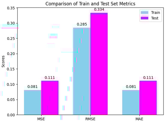
Figure 4.
The results for the model’s error metrics and goodness-of-fit indicators on the training and test sets.
Specifically, the negligible differences in MSE and RMSE between the training and test sets suggest a high degree of alignment between the model’s predictive accuracy on new data and on training data, indicating robust performance. The MAE values corroborate this finding, reflecting similar levels of prediction bias across both datasets and reinforcing the model’s consistency.
3.2. Test Set Evaluation Results
The results on the test data are presented in Figure 5. Specifically, the right-side image illustrates the outcomes for the Kepler crater, while the left-side image displays those for the Copernicus crater. In both images, green circles represent True Negatives (TNs) for primary craters (negative samples), yellow circles denote False Negatives (FNs) for secondary craters not classified as primary craters, red circles indicate False Positives (FPs), where primary craters are not classified as secondary craters, and blue circles represent True Positives (TPs) for correctly classified secondary craters (positive samples).
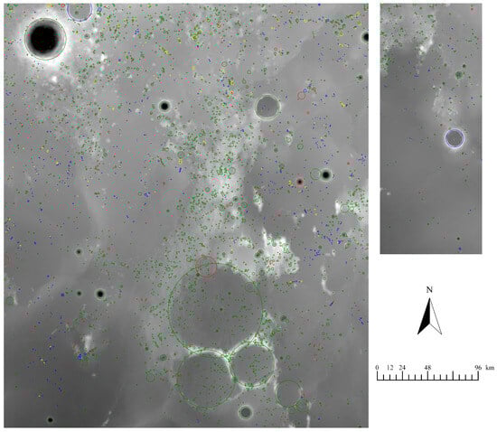
Figure 5.
Results on the test set for Copernicus crater (left) and Kepler crater (right). Green circles represent True Negatives (TNs) for primary craters (negative samples), yellow circles denote False Negatives (FNs) for secondary craters not classified as primary craters, red circles indicate False Positives (FPs), where primary craters are not classified as secondary craters, and blue circles represent True Positives (TPs) for correctly classified secondary craters (positive samples).
Table 4 presents the performance metrics of the CatBoost model, demonstrating its effectiveness in classifying primary and secondary craters, with particular attention to handling imbalanced data through the precision, recall, and F1 score. The detailed calculation methods for these performance metrics are provided in Appendix A.
Table 4.
Performance metrics for primary and secondary craters.
Figure 6 presents the precision–recall (P-R) curves for both the primary crater and secondary crater classes, along with their respective AUPRC values.
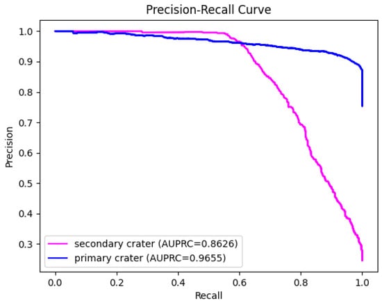
Figure 6.
P-R curve and AUPRC values for primary crater and secondary crater classes. The blue curve represents the P-R curve for the primary crater class, while the magenta curve represents the P-R curve for the secondary crater class.
The confusion matrix of the results is shown in Figure 7. This matrix displays the distribution of , , , and for the classification of craters into primary and secondary categories.The figure shows a significant difference in the number of samples between primary craters and secondary craters. The analysis indicated that the model performed well in the classification of primary craters, correctly classifying the majority of primary crater samples (a total of 2762), although 187 samples were classified as secondary craters. In contrast, the model’s accuracy for identifying secondary craters was relatively low. While it correctly classified 713 secondary crater samples, 249 secondary crater samples were classified as primary craters. This result aligned with the earlier performance metrics, highlighting that the model still encountered some challenges in distinguishing secondary craters accurately.
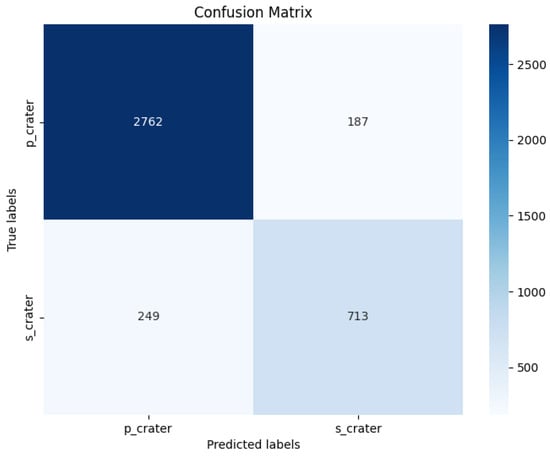
Figure 7.
Confusion matrix. s_crater represents secondary crater, while p_crater represents primary crater.
3.3. Variable Ablation Study
To verify the effectiveness of the newly proposed variables (density variables with Gaussian summation and two slope variables), a variable ablation study was conducted. In this experiment, we systematically removed or altered specific variables, including the newly introduced ones, and observed the corresponding changes in model accuracy and other performance metrics. The results of the variable ablation study are presented in Table 5.
Table 5.
Results of variable ablation experiment. A checkmark(✓) indicates that the corresponding variable was used in the experiment, while a dash(-) denotes that it was excluded.
The analysis of the ablation experiment revealed that the combination of density variable with Gaussian summation and average slope positively impacted model performance, enhancing precision for secondary craters and slightly improving both recall and precision for primary craters compared to the baseline. Similarly, the combination of density variables and slope angle demonstrated comparable benefits. However, when compared to the inclusion of only the density variable with Gaussian summation, the combination of the density variable with Gaussian summation and slope angle had a negative effect on certain model metrics, notably causing a decrease in recall by approximately 2%. Despite these mixed results, the overall accuracy improvement was somewhat limited, primarily due to the model misclassifying some secondary craters as primary craters.
When all additional variables were included, the model achieved its highest performance metric scores in the experiment, maintaining high recall and precision for primary craters, along with a noticeable improvement in the identification of secondary craters as well. This result indicates that the combination of multiple variables exhibited strong complementarity and synergy within the model, enhancing overall predictive performance. Overall, the variable ablation study confirmed the effectiveness of density variables with Gaussian summation, average slope, and slope angle in improving the model’s capability to distinguish between primary and secondary craters.
4. Discussion
4.1. Interpretation of CatBoost Model with SHAP
The SHAP Python package was executed using the trained machine learning model, and the SHAP value matrix was obtained. From this matrix, summary plots, dependence plots, and decision plots were generated. Summary plots provide a general view of variable importance by displaying the distribution of SHAP values across all samples. SHAP dependence plots show the contribution of a variable to each individual prediction, quantified by its SHAP value, illustrating the relationship between a specific variable and the model’s output while considering interactions with other variables. Decision plots visualize how individual variables contribute to the prediction for each sample, highlighting the cumulative impact of variables in decision making for a given prediction.
4.1.1. SHAP Summary Plot
Figure 8 presents the SHAP summary plot, which illustrates the variable importance in the CatBoost model based on SHAP values.
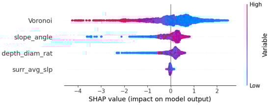
Figure 8.
SHAP summary plot for 4 individual variables.
The horizontal axis represents the SHAP values, and the color gradient from blue to red indicates changes in variable values from low to high. The vertical axis lists the variable names, with the top variables contributing more to the model and thus having high predictive power.
A comprehensive analysis revealed that the Voronoi variable had a wide range of influence on the SHAP value distribution, reflecting its significant role in model predictions under different variable values. At low variable values, its SHAP values were primarily positive, indicating that low Voronoi values tended to push the model towards predicting secondary craters. As the variable value increased, the SHAP value shifted to negative, meaning higher Voronoi values made the model more likely to predict primary craters. The significant variation in the variable’s impact highlighted its importance within the model.
In contrast, the SHAP value distribution for the depth-to-diameter ratio (depth_diam_rat) was more concentrated, indicating a relatively weaker effect on the model’s predictions. Low values tended to result in positive SHAP values, suggesting that small depth-to-diameter ratios pushed the model towards predicting secondary craters, while high values had little to no impact on the model. This demonstrated that the depth-to-diameter ratio provided a limited contribution to the model’s predictions, particularly in high value ranges.
The slope angle showed a similar pattern to depth-to-diameter ratio, with relatively small SHAP value variations. Low slope values resulted in positive SHAP values, indicating a tendency for the model to predict secondary craters under low-slope conditions. However, as slope values increased, their SHAP values approached zero, showing that higher slope values had a minimal impact on the model’s predictions.
Finally, the average slope (surr_avg_slp) exhibited the smallest variation in SHAP values, indicating that the surrounding average slope had a relatively weak influence on the model’s predictions. Regardless of the value, its SHAP values remained close to zero, showing that surrounding average slope had a negligible impact on the model’s output.
Overall, the Voronoi variable had the most significant impact among the four variables, while the depth-to-diameter ratio and slope angle had relatively weaker effects. The surrounding average slope contributed the least to the model. These results highlight the varying degrees of influence of each variable on the model’s predictions, emphasizing the key role of the Voronoi variable.
Figure 9 clearly shows the average SHAP values for each variable group, revealing their relative contributions to the model’s predictions. The chain density and cluster density variable groups display notably large negative SHAP values, indicating that both tend to shift the model’s predictions towards primary craters. The high negative SHAP values suggest that these variables have a significant impact on prediction outcomes, likely due to their precise description of crater density across different radius ranges.
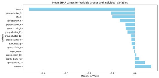
Figure 9.
The average SHAP values for variable groups and individual variables.
For variable groups that include parameters such as (group:cluster_6) (cluster density variable group with a = 3) and (group:chain_2) (chain density variable group with a = 2), the SHAP values reflect the effect of the Gaussian function’s parameter a. Parameter a controls the rate of density decay with distance, influencing the weight distribution of the variable’s values across different ranges. When the a value is small, the SHAP values for the cluster density variable groups are large, indicating that a small a allows the density to maintain high values over a wide range, extending the influence of these variables. Conversely, when the a value is large, the SHAP values for chain density variable groups increase, suggesting that chain density becomes more important in this case. Therefore, by adjusting the density decay, parameter a significantly affects the SHAP values, altering the model’s dependence on these variables and the resulting predictions.
Among the other variables, the depth-to-diameter ratio (depth_diam_rat) and average slope (surr_avg_slp) have relatively small average SHAP values, indicating that while these geometric variables hold some importance, their overall contribution to the model is limited. In contrast, the Voronoi variable has relatively large and positive SHAP values, suggesting that the area of the polygon generated around a crater’s center plays a significant role in predicting secondary craters. The SHAP value for the slope angle variable is close to zero, indicating that while this variable captures changes in surrounding terrain, it has a minimal influence on the model’s prediction outcomes.
Overall, density variables, particularly chain and cluster density, exhibit a significant impact on the model’s predictions, while geometric variables contribute relatively less to the model’s performance.
4.1.2. SHAP Dependence Plot
Figure 10 demonstrates the dependency between the depth-to-diameter ratio (depth_diam_rat) and average slope (surr_avg_slp) on the model’s SHAP values, revealing how these variables influence the model’s output. As the depth-to-diameter ratio increases, the SHAP values exhibit a trend of first rising and then falling, indicating that within the range of 0% to approximately 15%, a higher depth-to-diameter ratio pushes the model’s predictions towards secondary craters. Beyond this range, the influence of the depth-to-diameter ratio weakens, and it may even shift the model’s predictions more towards primary craters.
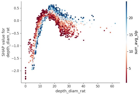
Figure 10.
Impact of depth-to-diameter ratio (depth_diam_rat) and average slope (surr_avg_slp) on model output.
The color gradient in the plot clearly reflects the impact of the average slope on the SHAP values. Points with higher average slopes (blue) are distributed in regions with higher SHAP values, while points with lower average slopes (red) cluster in areas with lower SHAP values. This suggests that, at steeper slopes, the depth-to-diameter ratio tends to push the model’s predictions towards primary craters. Under lower average slope conditions, smaller depth-to-diameter ratios are generally associated with more negative SHAP values, indicating that for flatter terrain, a decrease in the depth-to-diameter ratio makes the model more likely to predict secondary craters.
In cases of moderate average slopes, an increase in the depth-to-diameter ratio initially causes a rise in SHAP values, but this effect diminishes as the ratio continues to increase. In regions with high average slopes, large depth-to-diameter ratios more strongly influence the model towards predicting secondary craters, particularly when the depth-to-diameter ratio is in the mid-to-high range.
This complex interaction between the variables highlights the dynamic behavior of the model and clarifies how the depth-to-diameter ratio and average slope jointly affect the model’s output. Such variable interactions provide deeper insights into the nuanced ways the model makes its predictions.
To evaluate the impact of Gaussian-weighted cluster density on the SHAP values compared to those without Gaussian weighting, we selected the representative variable (cluster density with range = 100R and a = 3) and analyzed its influence on (cluster density with range = 100R, without a). The results are shown in Figure 11. From the figure, it is evident that when the values of are in the low-to-medium range (approximately 0 to 25), there is a strong linear negative correlation between the SHAP values of the unweighted density variable and the magnitude of the weighted density variable. Specifically, the larger the value, the smaller the SHAP value of , making the model more likely to predict primary craters. The SHAP value reaches its most negative point at a value of around 25, indicating that this is where has the greatest influence in pushing the model to predict primary craters.
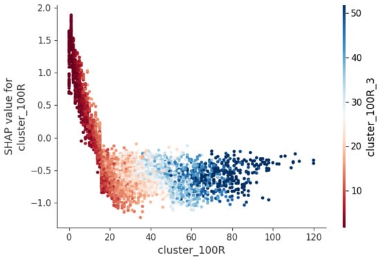
Figure 11.
Impact of and on model output.
However, as the value increases, especially beyond 50, the SHAP values gradually become more negative, suggesting that, at this point, the variable shifts the model’s predictions increasingly towards primary craters. Observing the color gradient and the distribution of points in the latter half of the graph, we find that as both and increase, the points become more densely clustered around SHAP = −0.5. This implies that as the variable values grow, the influence of the weighted density variable on the unweighted variable begins to weaken.
Overall, the interaction between and on the model’s output is complex. When the variable values are small, the influence of the Gaussian-weighted variable on the unweighted variable is more pronounced. However, as the variable values increase to a certain point, this influence gradually diminishes.
4.1.3. SHAP Decision Plot and Analysis of Misclassified Samples
Figure 12 presents the SHAP decision plot for misclassified samples, illustrating the cumulative impact of different variable groups on the model output through a red–blue gradient. In this figure, the upper variable groups (such as Voronoi, cluster, slope_angle, and chain) exhibit significant positive and negative contributions to the model output, with clear transitions between red and blue along the paths for these variable groups. This color change reflects the role of the variable groups in either elevating or lowering the model’s output values, where the red regions indicate a positive contribution from the variable groups, and the blue regions signify a negative contribution. The strong dependence of misclassified samples on these variable groups highlights their critical influence on the classification.
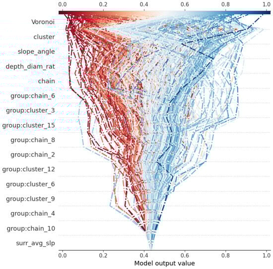
Figure 12.
SHAP decision plot for misclassified samples. The red color indicates that the corresponding variable drives the model’s prediction more toward classifying the sample as a primary crater, while the blue color suggests a stronger influence toward predicting it as a secondary crater.
The color transition from red to light blue along the central path of the image reflects the high uncertainty of the model near the classification boundary. This phenomenon indicates that the model’s predictions for these samples are not sufficiently clear, with the positive and negative influences of the variable groups being in a balanced state, resulting in the model struggling to make a definitive judgment about the sample categories. This uncertainty reveals the model’s ambiguous decisions regarding boundary samples, which may be one of the key reasons for incorrect classification.
At the bottom of the figure, variable groups such as , , and average slope() have a relatively minor impact on the model’s output. The limited variation in color along the paths for these variable groups indicates that their contributions to the model’s decisions are minimal.
Additionally, variable groups in the cluster and chain series ( , , etc.) exhibit similar color change patterns in the figure, suggesting that these variable groups may have a synergistic effect on similar samples. This consistency may stem from similarities in spatial structure or variable attributes within the data, reflecting the potential relationships and stability of these variable groups in the model’s decision-making process.
4.2. Comparison of the Variable Importance Derived from CatBoost and SHAP
We conducted an analysis and comparison of the variable importance scores derived from CatBoost’s get_feature_importance and SHAP, revealing notable differences in how these importance measures are computed and interpreted.
As shown in Figure 13, CatBoost’s get_feature_importance evaluates variable importance based on each variable’s contribution to minimizing the model’s loss function during training. Our results indicate that Voronoi, cluster, slope_angle (slope angle), and depth_diam_rat (depth-to-diameter ratio) exhibit the highest importance scores, suggesting their strong influence on the model’s decision-making process. Additionally, group:cluster_6 and chain also play a significant role, albeit to a slightly lesser extent.
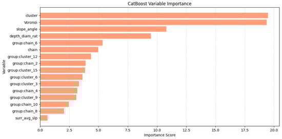
Figure 13.
Variable importance derived from CatBoost.
The results demonstrate that the cluster variable group has a significantly higher mean SHAP value than the other groups, indicating that it plays a dominant role in most individual sample predictions. Meanwhile, the Voronoi variable group, which was highly ranked in CatBoost’s importance analysis, exhibits a much lower mean SHAP value. This suggests that while it may be highly influential in certain cases, its overall contribution across all samples, is less significant. Furthermore, group:cluster_6 and group:chain_6 appear more influential in SHAP analysis than in CatBoost’s ranking, indicating that these variables may be particularly important for specific crater classifications rather than having a strong general influence.
A key advantage of SHAP is that it not only quantifies variable importance but also provides insight into how variables influence model predictions. Specifically, positive SHAP values indicate that a variable directs the model towards classifying a crater as secondary crater, whereas negative SHAP values suggest that the variable encourages classification as primary. This level of interpretability enables a deeper understanding of how individual variables drive classification, an aspect that CatBoost’s get_variable_importance does not inherently capture.
It is important to emphasize that the numerical values obtained from CatBoost’s variable importance and SHAP cannot be directly compared due to fundamental differences in their computation methods. CatBoost importance scores represent a variable’s contribution to minimizing the model’s loss function, while SHAP values quantify a variable’s average influence on individual predictions. Because the two methods have distinct computational principles and measurement scales, their importance scores should be analyzed within their respective contexts rather than compared numerically.
4.3. Partial Dependence Plot
In this section, we analyze the partial dependence plots (PDPs) of several key variables to reveal the trend in the effects of the changes in these variable values on the model’s predictions. By interpreting the PDP results for variables such as depth-to-diameter and Voronoi, we gained a more intuitive understanding of the model’s behavior across different variable values, enabling us to identify critical thresholds for these variables.
Figure 14 illustrates the partial dependent relationship between the depth-to-diameter ratio variable and the model’s predictions. It can be observed that as depth-to-diameter ratio increases, the probability of the model predicting a sample as a secondary crater (class 1) gradually rises. At low depth-to-diameter ratio values, the partial dependence values are relatively low, but when the depth-to-diameter ratio reaches the range of 10% to 20%, the prediction probability significantly increases. This trend suggests that, within this range, a high depth-to-diameter ratio increases the likelihood of a sample being classified as a secondary crater, indicating that this variable plays an important role in identifying secondary craters within this interval.
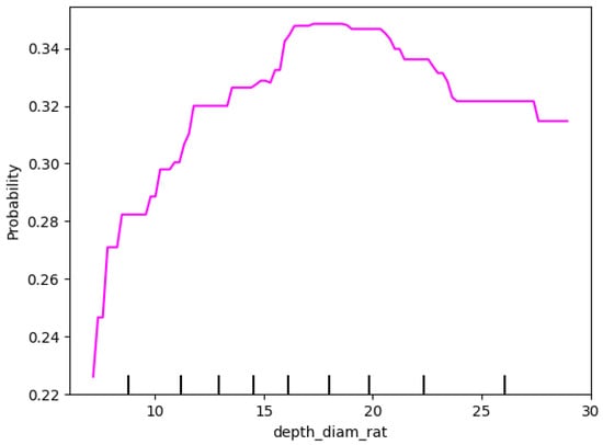
Figure 14.
Partial dependence plot of depth-to-diameter ratio (depth_diam_rat).
As depth-to-diameter ratio approaches 20%, the index tends to stabilize and slightly decline, suggesting this value is a critical threshold for the depth-to-diameter ratio. Beyond this threshold, the probability of predicting a secondary crater stabilizes or even slightly decreases. This implyiesthat when the depth-to-diameter ratio exceeds 20%, its influence on classifying a sample as a secondary crater reaches saturation, and further increases in this ratio have a limited, or even slightly negative, effect on the prediction. This threshold reflects a limiting role of the depth-to-diameter ratio in the classification of secondary craters.
The partial dependent relationship between the Voronoi variable and the model’s probability of classifying a sample as a secondary crater is presented in Figure 15. As the Voronoi value increases, the probability shows a significant downward trend, indicating a negative correlation between the Voronoi variable and the probability of classifying a sample as a secondary crater. Notably, within the low range of Voronoi values (≤10,000), the probability rapidly decreases from around 0.5 to below 0.3, suggesting that this variable is a strong discriminant for secondary craters in this range.
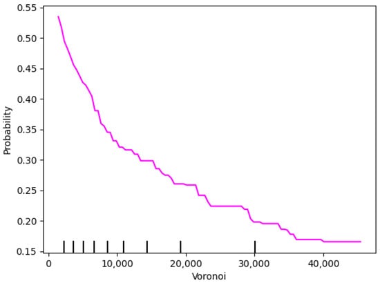
Figure 15.
Partial dependence plot of Voronoi variable.
When the Voronoi value approaches 20,000, the probability stabilizes around 0.25, indicating that at high Voronoi values, the variable’s impact on the probability of classifying a sample as a secondary crater weakens and reaches saturation. Beyond this point, further increases in the Voronoi value have a minimal influence on the prediction. This trend suggests that the Voronoi variable has a substantial contribution to the classification towards secondary craters within the low value range, while its influence on the classification result is relatively limited at high values.
In summary, a reasonable threshold for Voronoi is around 20,000, beyond which its contribution to the likelihood of classifying a sample as a secondary crater becomes stable. This observation aligns with previous findings on secondary craters, where large Voronoi values reduce the probability of samples being classified as secondary craters [].
Figure 16 presents the joint partial dependence relationship between the depth_diam_rat (depth-to-diameter ratio) and surr_avg_slp (average slope) variables on the model’s probability of predicting a sample as a secondary crater.
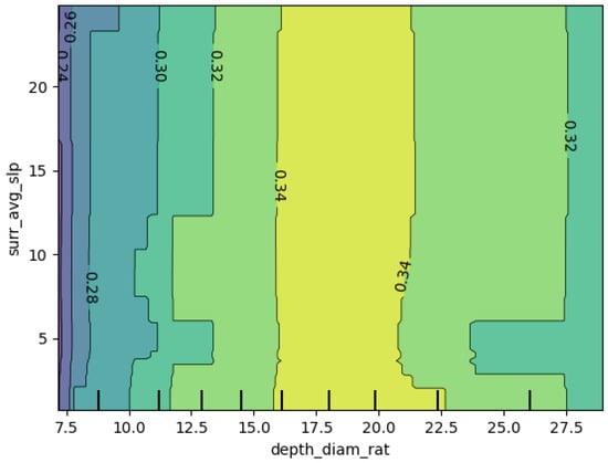
Figure 16.
The two-dimensional partial dependence plot which illustrates the interaction between the depth-to-diameter ratio (depth_diam_rat) and average slope (surr_avg_slp) on the predicted probability. Color gradients indicate the predicted probability, with light colors corresponding to high values.
At low depth-to-diameter ratios (approximately 7.5% to 15%), the predicted outcome remains low, particularly when the average slope is also moderate, with values between 0.26 and 0.30. As the depth-to-diameter ratio increases, especially in the range of 16 to 20, the predicted value shows a gradual rise, reaching approximately 0.34 at any average slope value.
When the depth-to-diameter ratio reaches the range of 15% to 20% and the average slope is at a moderate level, the probability peaks at approximately 0.34, suggesting that this variable combination enhances the model’s ability to recognize secondary craters. However, when the depth-to-diameter ratio exceeds 20%, the probability stabilizes and slightly decreases with further increases, even if the average slope remains moderate, indicating that the incremental impact on probability has reached saturation.
The co-dependent depth-to-diameter ratio and average slope reveals the potential formation characteristics of secondary craters: a combination of a moderate depth-to-diameter ratio and an average slope is more favorable for identifying secondary craters, while higher depth-to-diameter ratios have a relatively limited contribution to secondary crater classification.
4.4. Effectiveness Verification of Label Correction Approach
To validate the effectiveness of our label correction approach in addressing the dataset contamination caused by incomplete annotations of secondary craters, we designed an experimental framework.
The procedure is as follows:
- Sampling Class 1 Instances: For each fold in the cross-validation, 10% of the samples originally labeled as class 1 (secondary craters), which were not modified during the cross-validation process, are randomly selected. The labels of these randomly selected samples are then changed from class 1 to class 0 (primary craters). These samples are used as a representative subset for further evaluation.
- Model Training and Prediction: A classifier is trained on the remaining portion of the data, excluding the selected 10%, and predictions are made on the high-confidence class 1 samples.
- Confidence Thresholding: In the CatBoost model, a sample is classified as class 1 (secondary crater) if the predicted probability for class 1 exceeds 0.5. Therefore, the model’s predicted probabilities are evaluated, and samples with a predicted probability greater than 0.5 are considered high-confidence predictions.
- Calculation of High-Confidence Ratio: The ratio of high-confidence samples—those with a predicted probability exceeding 0.5—to the total number of samples in the 10% subset is computed for each fold. This ratio serves as a key metric for quantifying the success of the cross-validation strategy in correctly classifying secondary craters. The purpose of this step is to evaluate the model’s ability to correctly recover mislabeled or missed labels when using the label correction approach, thereby assessing how effectively the model can identify and correct misclassifications.
- Average High-Confidence Ratio Across Folds: After evaluating each fold, the average ratio of high-confidence samples across all folds is calculated. This provides an aggregated measure of the overall impact of the pseudo-labeling approach on model performance.
The average ratio of high-confidence samples was 0.7477, while the recall of the model tested on the dataset applying the cross-validation approach was 0.7412, resulting in a difference of 0.0065 (approximately 0.65%). This slight yet meaningful difference provides evidence for the effectiveness of the cross-validation-based approach implemented in this study. Moreover, it demonstrates that even if a portion (10%) of secondary craters is mislabeled or missed, there remains a 74.77% probability of correctly identifying them. This finding suggests that the model exhibits a certain degree of generalization ability, maintaining robust performance despite partial label contamination.
4.5. Comparison with Previous Work
In this study, several key advancements were made compared to the work presented in []. We introduced several new features, such as slope and density with Gaussian Summation, which provide more detailed information on crater morphology and improve the model’s ability to distinguish between crater types. Additionally, while [] used the Robbins 2018 [] and Guo2018 [] datasets, we utilized Robbins 2018 [] and Singer 2020 [] datasets, with our research focusing on the Kepler and Copernicus regions as opposed to []’s primary focus on the Orientale region.
Another improvement lies in the emphasis on model interpretability. In contrast to [], which did not explore this aspect, we apply SHAP (SHapley Additive exPlanations) and Partial Dependence Plots (PDP) to conduct a comprehensive analysis of feature importance. These interpretability methods provide valuable insights into the contribution of individual features to the model’s classification performance, thereby increasing the transparency and explanatory power of our results.
4.6. Considerations Regarding Small Craters
This study primarily focused on the detection and classification of mid- to large-sized craters, for which the available SLDEM data with a spatial resolution of 59 m/pixel provided sufficient detail for effective feature extraction. The morphological, contextual, and density-based features derived from this resolution were well suited for craters in this study.
However, for very small craters, the spatial resolution constrains the ability to extract reliable morphological and contextual information, which makes accurate classification more challenging. Despite this, it is worth noting that, in the Singer 2020 [] dataset used in this study, approximately half of the secondary craters have diameters ranging from 800 m to 1 km. These craters, though approaching the lower limit of what can be effectively resolved by the SLDEM data, still provided valuable instances for evaluating the model’s ability to handle relatively small craters under the current resolution.
Moreover, as demonstrated by our label correction experiment, the proposed method retains a degree of pability to identify and reclassify underrepresented or unlabeled secondary craters, including small craters that are challenging due to both resolution limitations and dataset contamination. This suggests that the model can generalize reasonably well, even in the presence of incomplete annotations and suboptimal resolution for smaller crater classification.
Given these constraints, this study focused on regions such as Kepler and Copernicus, where most of the annotated secondary craters are of sufficiently large size to be well resolved in the DEM data. Extending this approach to areas dominated by smaller craters will likely require further methodological improvements. In future work, we intend to incorporate higher-resolution datasets, such as TC morning, and explore multi-scale feature extraction strategies to enhance the model’s ability to classify craters across a broader range of sizes, particularly targeting smaller secondary craters.
5. Conclusions
This study developed a high-performance crater classification model using Digital Elevation Model (DEM) data to better interpret the model’s predictions. We first processed the DEM data and extracted crater variables, followed by the application of the CatBoost algorithm for crater classification. The CatBoost model achieved an F1 score of 0.7658 and a recall rate of 0.7412, demonstrating the effectiveness of the method for crater classification tasks.
Subsequently, we introduced the SHAP method, which provided valuable insights into the overall behavior of the model by revealing the relationships between crater variables and classification. In particular, our analysis highlighted several key factors that contribute significantly to crater classification. For instance, variables such as Voronoi, depth-to-diameter ratio, and slope angle exhibited a strong influence on the classification decisions. Similarly, crater density contributed significantly to distinguishing impact-related formations. Additionally, the use of partial dependence plots (PDPs), which depict the predicted probability as a function of a single variable while marginalizing over the others, allowed us to analyze the influence of individual variables across different value ranges. This approach enhanced our understanding of how these factors impact the likelihood of a crater being classified as primary or secondary. For example, the PDP results indicated that secondary craters tend to be associated with a high depth-to-diameter ratio (expressed as percentages) and small Voronoi cell areas compared to primary craters.
The important insights gained from this study underscore the potential of combining advanced machine learning techniques with methods to unravel the inherently complex relationships among lunar crater characteristics. These findings not only enhance our understanding of crater formation and evolution but also pave the way for more refined analyses in planetary science.
Explainable AI offers a powerful tool for planetary geology, enabling the development of frameworks applicable to other planetary bodies, such as Mars, where impact crater classification is essential for understanding surface evolution. Future research could enhance classification performance by incorporating advanced machine learning techniques and ensemble methods while extending this approach to other planetary surfaces to deepen insights into planetary geologic processes and support upcoming exploration missions.
Additionally, we will explore methods such as advanced data augmentation and annotation interpolation techniques to improve variable extraction in sparse regions in future work. Specifically, we plan to investigate techniques to augment the annotations in the Orientale region, such as using semi-supervised learning or active learning, to generate more reliable secondary crater annotations. This would help balance the dataset and improve variable extraction in regions with sparse crater data.
Author Contributions
Conceptualization, M.Z. and J.L.; methodology, M.Z. and J.L.; software, M.Z.; validation, M.Z. and W.H.; formal analysis, M.Z., X.Z. and Y.X.; investigation, M.Z. and W.H.; resources, M.Z. and J.L.; data curation, M.Z. and J.L.; writing—original draft preparation, M.Z.; writing—review and editing, M.Z., J.L., X.Z. and Y.X.; visualization, M.Z.; supervision, J.L., X.Z. and Y.X.; project administration, M.Z. and J.L.; funding acquisition, J.L., X.Z. and Y.X. All authors have read and agreed to the published version of the manuscript.
Funding
This work was supported by the National Natural Science Foundation of China (grants 12103020 and 12363009), the Science and Technology Development Fund (FDCT) of Macau (Grants 0021/2024/RIA1, 0158/2024/AFJ), the Natural Science Foundation of Jiangxi Province (grant 20224BAB211011), the Open Project Program of State Key Laboratory of Lunar and Planetary Sciences (Macau University of Science and Technology) (Macau FDCT grant No. 002/2024/SKL), the Youth Talent Project of the Science and Technology Plan of Ganzhou (grants 2022CXRC9191 and 2023CYZ26970), and the Jiangxi Province Graduate Innovation Special Fund Project (grants YC2023-S672 and YC2024-S529).
Data Availability Statement
SLDEM data can be accessed from the Planetary Data System LOLA data node (https://imbrium.mit.edu/EXTRAS/SLDEM2015/). The data from Robbins 2018 are available at https://astrogeology.usgs.gov/search/map/moon_crater_database_v1_robbins. Additionally, the secondary data files from Singer 2020, which include all secondary crater diameters and locations, can be found at this site (https://doi.org/10.6084/m9.figshare.11299319).
Conflicts of Interest
The authors declare no conflicts of interest.
Appendix A
To comprehensively evaluate the performance of the CatBoost model in this study, a series of metrics were employed to measure its effectiveness in crater classification tasks. The selected evaluation metrics included the following:
Recall measures the model’s ability to correctly identify positive class samples. It is defined as the ratio of True Positives () to the sum of True Positives and False Negatives (), which can be expressed as
Precision emphasizes the accuracy of the model when predicting positive instances, indicating the proportion of samples predicted as positive that are actually positive. It is defined as the ratio of True Positives () to the sum of True Positives and False Positives (), expressed as
F1 score is the harmonic mean of precision and recall, used to strike a balance between the two metrics. It is particularly useful when there is a need to find a trade off between precision and recall and is especially effective for imbalanced datasets. The F1 score is defined as
Kappa is used to measure the agreement between the model’s predictions and the actual classification results, while accounting for the possibility of agreement occurring by chance. The calculation formula for Kappa is
where represents the observed accuracy, which is the proportion of instances where the model’s predictions match the actual classifications. is the expected accuracy due to random chance, reflecting the probability that the predictions and actual classifications agree purely by coincidence.
The Kappa value ranges from −1 to 1, with higher values indicating more reliable model predictions.
Accuracy is one of the most commonly used evaluation metrics, representing the proportion of correctly classified samples by the model. The formula for calculating accuracy is
P-R curve (precision–recall curve) illustrates the trade-off between precision and recall across different decision thresholds. It is useful with imbalanced datasets, where the model’s ability to correctly identify the minority class (positive class) is critical.
AUPRC (area under the precision–recall curve) represents the area under the precision–recall curve and is used to assess the overall performance of a model across all thresholds. A higher AUCPR indicates better model performance in detecting and classifying positive samples.
Confusion matrix is a fundamental evaluation tool for classification models, displaying the relationship between the true labels and the predicted labels in a matrix format. It consists of four elements: , , , and . The confusion matrix not only provides the underlying data to compute various performance metrics, such as precision, recall, F1 score, and accuracy, but also visually reflects the model’s classification performance across different sample classes.
For a binary classification problem, the confusion matrix can be represented as follows:
References
- Wilhelms, D.E.; John, F.; Trask, N. The Geologic History of the Moon; U.S. Government Printing Office: Washington, DC, USA, 1987. [Google Scholar]
- Head, J.W.; Fassett, C.I.; Kadish, S.J.; Smith, D.E.; Zuber, M.T.; Neumann, G.A.; Mazarico, E.M. Global Distribution of Large Lunar Craters: Implications for Resurfacing and Impactor Populations. Science 2010, 329, 1504–1507. [Google Scholar] [CrossRef] [PubMed]
- Dundas, C.M.; McEwen, A.S. Rays and secondary craters of Tycho. Icarus 2007, 186, 31–40. [Google Scholar] [CrossRef]
- Bierhaus, E.B.; McEwen, A.S.; Robbins, S.J.; Singer, K.N.; Dones, L.; Kirchoff, M.R.; Williams, J.P. Secondary craters and ejecta across the solar system: Populations and effects on impact-crater-based chronologies. Meteorit. Planet. Sci. 2018, 53, 638–671. [Google Scholar] [CrossRef]
- Xiao, Z. Size-frequency distribution of different secondary crater populations: 1. Equilibrium caused by secondary impacts. J. Geophys. Res. Planets 2016, 121, 2404–2425. [Google Scholar] [CrossRef]
- Luo, F.; Xiao, Z.; Wang, Y.; Ma, Y.; Xu, R.; Wang, S.; Xie, M.; Wu, Y.; Deng, Q.; Ma, P. The Production Population of Impact Craters in the Chang’E-6 Landing Mare. Astrophys. J. Lett. 2024, 974, L37. [Google Scholar] [CrossRef]
- Su, Y.; Xu, L.; Zhu, M.H.; Cui, X.L. Composition and Provenance of the Chang’e-6 Lunar Samples: Insights from the Simulation of the Impact Gardening Process. Astrophys. J. Lett. 2024, 976, L30. [Google Scholar] [CrossRef]
- Werner, S.C.; Bultel, B.; Rolf, T. Review and Revision of the Lunar Cratering Chronology—Lunar Timescale Part 2. Planet. Sci. J. 2023, 4, 147. [Google Scholar] [CrossRef]
- Xu, Z.; Guo, D.; Liu, J. Maria Basalts Chronology of the Chang’E-5 Sampling Site. Remote Sens. 2021, 13, 1515. [Google Scholar] [CrossRef]
- Xu, L.; Qiao, L. Formation age of the Rima Sharp sinuous rill on the Moon, source of the returned Chang’e-5 samples. Astron. Astrophys. 2022, 657, A42. [Google Scholar] [CrossRef]
- Herrera, C.; Carry, B.; Lagain, A.; Vavilov, D.E. Binary craters on Ceres and Vesta and implications for binary asteroids. Astron. Astrophys. 2024, 688, A176. [Google Scholar] [CrossRef]
- Li, X.; Vincent, J.-B.; Weller, R.; Zachmann, G. Numerical approach to synthesizing realistic asteroid surfaces from morphological parameters. Astron. Astrophys. 2022, 659, A176. [Google Scholar] [CrossRef]
- Martin, A.C.; Denevi, B.W.; Speyerer, E.J.; Boyd, A.K.; Brown, H.M. Imaging in Shadows: A Comparison of Craters Observed in Primary and Secondary Illumination with the Lunar Reconnaissance Orbiter Camera. Planet. Sci. J. 2024, 5, 207. [Google Scholar] [CrossRef]
- Wueller, L.; Iqbal, W.; Frueh, T.; van der Bogert, C.H.; Hiesinger, H. Geologic History of the Amundsen Crater Region Near the Lunar South Pole: Basis for Future Exploration. Planet. Sci. J. 2024, 5, 147. [Google Scholar] [CrossRef]
- Rivera-Valentín, E.G.; Fassett, C.I.; Denevi, B.W.; Meyer, H.M.; Neish, C.D.; Morgan, G.A.; Cahill, J.T.S.; Stickle, A.M.; Patterson, G.W. Mini-RF S-band Radar Characterization of a Lunar South Pole-crossing Tycho Ray: Implications for Sampling Strategies. Planet. Sci. J. 2024, 5, 94. [Google Scholar] [CrossRef]
- Chang, Y.; Xiao, Z.; Liu, Y.; Cui, J. Self-Secondaries Formed by Cold Spot Craters on the Moon. Remote Sens. 2021, 13, 1087. [Google Scholar] [CrossRef]
- Xu, X.; Ye, L.; Kang, Z.; Jiang, W.; Luan, D.; Zhang, D. The Identification of Secondary Craters based on the Distribution of Iron Element on Lunar Surface. Geomat. Inf. Sci. Wuhan Univ. 2025, 47, 287–295. [Google Scholar] [CrossRef]
- Basilevsky, A.; Kozlova, N.; Zavyalov, I.; Karachevtseva, I.; Kreslavsky, M. Morphometric studies of the Copernicus and Tycho secondary craters on the moon: Dependence of crater degradation rate on crater size. Planet. Space Sci. 2018, 162, 31–40. [Google Scholar] [CrossRef]
- O’Brien, P.; Byrne, S. Degradation of the Lunar Surface by Small Impacts. Planet. Sci. J. 2022, 3, 235. [Google Scholar] [CrossRef]
- Guo, D.; Liu, J.; Head, J.W., III; Kreslavsky, M.A. Lunar Orientale Impact Basin Secondary Craters: Spatial Distribution, Size-Frequency Distribution, and Estimation of Fragment Size. J. Geophys. Res. Planets 2018, 123, 1344–1367. [Google Scholar] [CrossRef]
- Salih, A.; Lompart, A.; Grumpe, A.; Wöhler, C.; Hiesinger, H. Automatic detection of secondary craters and mapping of planetary surface age based on lunar orbital images. Int. Arch. Photogramm. Remote Sens. Spat. Inf. Sci. 2017, XLII-3/W1, 125–132. [Google Scholar] [CrossRef]
- McEwen, A.S.; Bierhaus, E.B. The importance of secondary cratering to age constraints on planetary surfaces. Annu. Rev. Earth Planet. Sci. 2006, 34, 535–567. [Google Scholar] [CrossRef]
- Bierhaus, E.; Chapman, C.; Merline, W. Secondary craters on Europa and implications for cratered surfaces. Nature 2005, 437, 1125–1127. [Google Scholar] [CrossRef] [PubMed]
- Yamamoto, S.; Matsunaga, T.; Nakamura, R.; Sekine, Y.; Hirata, N.; Yamaguchi, Y. An Automated Method for Crater Counting Using Rotational Pixel Swapping Method. IEEE Trans. Geosci. Remote Sens. 2017, 55, 4384–4397. [Google Scholar] [CrossRef]
- Benedix, G.K.; Lagain, A.; Chai, K.; Meka, S.; Anderson, S.; Norman, C.; Bland, P.A.; Paxman, J.; Towner, M.C.; Tan, T. Deriving Surface Ages on Mars Using Automated Crater Counting. Earth Space Sci. 2020, 7, e2019EA001005. [Google Scholar] [CrossRef]
- Wang, Y.; Wu, B.; Xue, H.; Li, X.; Ma, J. An Improved Global Catalog of Lunar Impact Craters (≥1 km) with 3D Morphometric Information and Updates on Global Crater Analysis. J. Geophys. Res. Planets 2021, 126, e2020JE006728. [Google Scholar] [CrossRef]
- Lin, X.; Zhu, Z.; Yu, X.; Ji, X.; Luo, T.; Xi, X.; Zhu, M.; Liang, Y. Lunar Crater Detection on Digital Elevation Model: A Complete Workflow Using Deep Learning and Its Application. Remote Sens. 2022, 14, 621. [Google Scholar] [CrossRef]
- Lagain, A.; Servis, K.; Benedix, G.K.; Norman, C.; Anderson, S.; Bland, P.A. Model Age Derivation of Large Martian Impact Craters, Using Automatic Crater Counting Methods. Earth Space Sci. 2021, 8, e2020EA001598. [Google Scholar] [CrossRef]
- Fairweather, J.H.; Lagain, A.; Servis, K.; Benedix, G.K.; Kumar, S.S.; Bland, P.A. Automatic Mapping of Small Lunar Impact Craters Using LRO-NAC Images. Earth Space Sci. 2022, 9, e2021EA002177. [Google Scholar] [CrossRef]
- Latorre, F.; Spiller, D.; Sasidharan, S.; Basheer, S.; Curti, F. Transfer learning for real-time crater detection on asteroids using a Fully Convolutional Neural Network. Icarus 2023, 394, 115434. [Google Scholar] [CrossRef]
- Vega García, M.; Aznarte, J.L. Shapley additive explanations for NO2 forecasting. Ecol. Inform. 2020, 56, 101039. [Google Scholar] [CrossRef]
- Lundberg, S.M.; Lee, S.I. A unified approach to interpreting model predictions. In Proceedings of the 31st International Conference on Neural Information Processing Systems, NIPS’17, Red Hook, NY, USA, 4–9 December 2017; pp. 4768–4777. [Google Scholar]
- Han, L.; Yang, G.; Yang, X.; Song, X.; Xu, B.; Li, Z.; Wu, J.; Yang, H.; Wu, J. An explainable XGBoost model improved by SMOTE-ENN technique for maize lodging detection based on multi-source unmanned aerial vehicle images. Comput. Electron. Agric. 2022, 194, 106804. [Google Scholar] [CrossRef]
- Friedman, J.H. Greedy function approximation: A gradient boosting machine. Ann. Stat. 2001, 29, 1189–1232. [Google Scholar]
- Liu, Q.; Cheng, W.; Yan, G.; Zhao, Y.; Liu, J. A Machine Learning Approach to Crater Classification from Topographic Data. Remote Sens. 2019, 11, 2594. [Google Scholar] [CrossRef]
- Robbins, S.J. A New Global Database of Lunar Impact Craters >1–2 km: 1. Crater Locations and Sizes, Comparisons with Published Databases, and Global Analysis. J. Geophys. Res. Planets 2019, 124, 871–892. [Google Scholar] [CrossRef]
- Singer, K.N.; Jolliff, B.L.; McKinnon, W.B. Lunar Secondary Craters and Estimated Ejecta Block Sizes Reveal a Scale-Dependent Fragmentation Trend. J. Geophys. Res. Planets 2020, 125, e2019JE006313. [Google Scholar] [CrossRef]
- Barker, M.; Mazarico, E.; Neumann, G.; Zuber, M.; Haruyama, J.; Smith, D. A new lunar digital elevation model from the Lunar Orbiter Laser Altimeter and SELENE Terrain Camera. Icarus 2016, 273, 346–355. [Google Scholar] [CrossRef]
- Chen, R.; Xu, Y.; Xie, M.; Zhang, L.; Niu, S.; Bugiolacchi, R. Sub-surface stratification and dielectric permittivity distribution at the Chang’E-4 landing site revealed by the lunar penetrating radar. Astron. Astrophys. 2022, 664, A35. [Google Scholar] [CrossRef]
- Prokhorenkova, L.; Gusev, G.; Vorobev, A.; Dorogush, A.V.; Gulin, A. CatBoost: Unbiased boosting with categorical features. Adv. Neural Inf. Process. Syst. 2018, 31. [Google Scholar]
- Štrumbelj, E.; Kononenko, I. Explaining prediction models and individual predictions with feature contributions. Ann. Stat. 2013, 41, 647–665. [Google Scholar]
- Ribeiro, M.T.; Singh, S.; Guestrin, C. “Why Should I Trust You?”: Explaining the Predictions of Any Classifier. In Proceedings of the 22nd ACM SIGKDD International Conference on Knowledge Discovery and Data Mining, San Francisco, CA, USA, 13–17 August 2016; Association for Computing Machinery: New York, NY, USA, 2016; pp. 1135–1144. [Google Scholar] [CrossRef]
Disclaimer/Publisher’s Note: The statements, opinions and data contained in all publications are solely those of the individual author(s) and contributor(s) and not of MDPI and/or the editor(s). MDPI and/or the editor(s) disclaim responsibility for any injury to people or property resulting from any ideas, methods, instructions or products referred to in the content. |
© 2025 by the authors. Licensee MDPI, Basel, Switzerland. This article is an open access article distributed under the terms and conditions of the Creative Commons Attribution (CC BY) license (https://creativecommons.org/licenses/by/4.0/).