Article

Exploring Stand Parameters Using Terrestrial Laser Scanning in Pinus tabuliformis Plantation Forests

1
School of Soil and Water Conservation, Beijing Forestry University, Beijing 100083, China
2
Jixian National Forest Ecosystem Observation and Research Station, CNERN, School of Soil and Water Conservation, Beijing Forestry University, Linfen 041000, China
3
Key Laboratory of State Forestry Administration for Soil and Water Conservation, College of Soil and Water Conservation, Beijing Forestry University, Beijing 100083, China
4
ICT Forestry Division, Forest Consulting Technology Department, Asia Air Survey Co., Ltd., Kawasaki 215-0004, Japan
*
Author to whom correspondence should be addressed.
Remote Sens. 2025, 17(7), 1228; https://doi.org/10.3390/rs17071228
Submission received: 27 February 2025 / Revised: 24 March 2025 / Accepted: 27 March 2025 / Published: 30 March 2025
(This article belongs to the Special Issue Lidar for Forest Parameters Retrieval)

Abstract

:
The rapid and precise acquisition of forest stand parameters is a key challenge in forest resource assessment. Terrestrial laser scanning (TLS) provides a fast and accurate method, but its accuracy is influenced by factors like tree segmentation parameters. This study focuses on Pinus tabuliformis plantations in the Caijiachuan watershed, Jixian, Shanxi, on the Loess Plateau. Based on field survey data, including tree number, height (H), diameter at breast height (DBH), and biomass, high-precision point cloud data were acquired using TLS. A comparative shortest path (CSP) algorithm was used for individual tree segmentation to investigate the effect of parameter selection on measurement accuracy. The results show that minimum tree height has a significant impact on segmentation accuracy. As the minimum tree height increased from 3.0 to 5.5 m, the recall rate (R) decreased while the precision (P) increased. The highest precision (F-score = 0.9470) and biomass estimation accuracy (0.9066) were obtained with a minimum tree height of 4.5 m, and the best extraction accuracies for H and DBH (0.9677 and 0.9518) were obtained at 5.0 m. Optimizing the minimum tree height parameter improves segmentation accuracy, thereby enhancing the use of TLS for soil and water conservation on the Loess Plateau.

Graphical Abstract

1. Introduction

Forests are the backbone of terrestrial ecosystems [1] and a fundamental resource for human survival [2]. Forest inventories are a vital means of assessing forest resource quantity, quality, and distribution [3]. Stand parameters, such as diameter at breast height (DBH), tree height (H), and biomass, are the main content during forest resource surveys and are also key indicators reflecting the spatial structure of forests, the health of forest growth, and the stability of forest ecosystems [4]. Traditional forest stand parameter surveys often rely on manual field measurements, which is not only time-consuming and labor-intensive but also presents challenges to ensuring the timeliness of the data, especially when rapid and accurate monitoring of large areas of forests is required; the limitations of the traditional methods are more significant [5]. Consequently, obtaining forest stand parameters quickly and accurately has become a substantial challenge in forest resource surveys.
With the rapid advancement of remote sensing technology, various methods and equipment, such as optical remote sensing [6,7], microwave remote sensing [8,9], and LiDAR [10,11], have been widely applied in extracting forest stand parameters. Optical remote sensing is currently the most commonly used method; however, its signals struggle to penetrate clouds, water vapor, and diverse atmospheric conditions, significantly affecting the acquisition of optical remote sensing imagery. Additionally, in densely forested areas, where optical remote sensing data may become saturated, accurately capturing information about ground-level or understory vegetation is challenging [12]. In contrast, microwave remote sensing is unaffected by weather conditions and can operate effectively under various climatic conditions [13]. However, the complex terrain found in forests can interfere with the microwave signals, making it difficult to mitigate this disruption altogether [14]. In this context, LiDAR has emerged as a crucial tool for remote sensing applications in extracting forest stand parameters. Its strong penetration capabilities, rapid acquisition of high-precision 3D data, and adaptability to complex terrains make it especially useful [15].
In recent decades, various LiDAR technologies, including satellite-borne [16], airborne [17], vehicle-mounted [18], and terrestrial laser scanning (TLS) [19], have been increasingly used to analyze and extract parameters of forest stands. Each type of LiDAR, however, faces unique challenges in its application. Satellite-borne LiDAR offers global coverage but has low resolution, making it difficult to obtain detailed information about the ground, particularly in dense forests [20]. Airborne LiDAR can cover vast areas, but accurately capturing information from the lower layers of the forest canopy is difficult due to shading from the canopy itself [21]. Vehicle-mounted LiDAR depends on road infrastructure, making it difficult to use in rugged or untraveled forested areas [22]. TLS employs a bottom–up static scanning method through fixed stations, enabling it to accurately capture the three-dimensional structures of forests and provide high-resolution data. Its deployment is also less restricted by terrain conditions [23]. As a result, TLS has become increasingly beneficial for researching, managing, and planning forest resources, making it a central focus of ongoing studies in the field [24].
Biomass is a crucial parameter for evaluating forest ecosystems’ productivity, carbon sink function, and health. It is essential in developing sustainable forest management and utilization strategies [25]. As key stand parameters, DBH and H not only directly reflect tree growth and forest structure but also provide essential data for biomass estimation [26]. Consequently, the swift and precise measurement of DBH and H, along with biomass estimation based on these measurements using TLS, has become a key area of research in forest resource surveys. Accurate tree segmentation is crucial for extracting stand parameters due to forests’ dense and complex nature [27].
Recent studies have made significant advances in individual tree segmentation, both nationally and internationally. In terms of data structure, most existing studies have used methods based on rasterization [28,29], voxelization [30,31], and point cloud data [32,33] for individual tree segmentation. Point cloud rasterization enhances analysis efficiency and visualization by converting 3D data into 2D [34]. However, the rasterization process is resolution-dependent, which may result in the loss of point cloud details, thereby impacting the accuracy of individual tree segmentation [35]. When compared to rasterization, voxelization is more effective at preserving 3D information, minimizing noise, and enhancing adaptability and accuracy in complex forest structures [36]. However, this method can be computationally demanding and may result in boundary blurring and loss of detail if the voxel size is not chosen correctly [37]. Segmentation that directly utilizes point cloud data retains the original 3D coordinate information, avoids the resolution limitations associated with rasterization, and eliminates accuracy loss from inappropriate voxel sizes during voxelization, thereby maximizing the precision of individual tree segmentation [38].
In terms of segmentation algorithms, Huang [39] et al. used a voxel-based labeled neighborhood search method to segment roadside trees with high accuracy, which may not apply to forests with intersecting and irregular canopy shapes because roadside trees have more uniform canopy shapes and usually do not have intersecting canopies. Yu [40] et al. proposed an improved region-growing algorithm, and the results of the study showed that the algorithm can effectively handle the case of intersecting and irregularly shaped tree crowns, showing better robustness and accuracy. However, the algorithm may be sensitive to the selection of initial seed points, which leads to unstable segmentation results and limits its applicability under different environmental conditions. Mu et al. [41] proposed a multi-scale spatial enhancement network and rectangular convolution self-attention fusion method, which can enhance feature saliency and improve segmentation accuracy in complex forest environments. However, these methods usually rely on large-scale training data for optimization, and in sample-scale studies with limited labeled data, deep learning methods may be difficult to generalize, leading to unstable segmentation results. Tao et al. [42] proposed a comparative shortest path (CSP) algorithm inspired by ecological theory, which starts with density-dependent spatial clustering using the density-based spatial clustering of applications with noise (DBSCAN) method to identify tree trunks. In contrast, the CSP method does not rely on large-scale training data but is based on density-dependent spatial clustering (DBSCAN) combined with the shortest path calculation from the crown point to the trunk, which can effectively deal with complex situations, such as overlapping crowns and irregular crown morphology at the sample plot scale. In addition, the CSP method can optimize the canopy segmentation in a local range in the sample scale high-resolution LiDAR data, improve the accuracy, and reduce the dependence on the initial seed points, which improves stability.
Based on research area, most of the studies on forest stand parameter extraction through TLS are concentrated in tropical rainforests [43,44], subtropical forests [45,46], urban forests [47,48], and other areas with flat topography. In contrast, relatively few studies have been conducted on the Loess Plateau region, which is a region of large topographic undulations, fragile ecological environments, and severe erosion, and most of the existing studies have been focused on the monitoring of soil erosion in the Loess Plateau [49,50]. Pinus tabuliformis has become a dominant tree species for afforestation in the Loess Plateau region due to its high survival rate, strong germination capacity, well-developed root system, and drought resistance [51]. Rapid and accurate extraction of forest stand parameters of P. tabuliformis forests is conducive to assessing its growth status, optimizing forest management, promoting ecological restoration, and providing a scientific basis for local vegetation management measures, thus promoting the construction of a sustainable environment.
In conclusion, this study focuses on an artificial P. tabuliformis forest in the Caijiachuan watershed of Jixian, Shanxi, in the southeastern section of the Loess Plateau. TLS was used to collect remote sensing data, while the CSP algorithm was used to segment individual trees. This study intends to achieve the following objectives. (1) TLS point cloud data were segmented into individual trees using the CSP algorithm, with a focus on examining how the minimum tree height parameter influences segmentation accuracy. The aim is to identify the optimal segmentation under varying minimum tree height settings and enhance the precision and stability of individual tree segmentation. (2) By analyzing the impact of various minimum tree height settings on the extraction of DBH and H, the accuracy of parameter extraction was optimized, providing a reference for the precise extraction of forest stand parameters. (3) To verify the effects of different minimum tree height settings on the accuracy of biomass estimation, to determine the optimal method for biomass estimation in the region, and to provide fast and accurate technical support for forest resource investigation and ecological management in the area.

2. Materials and Methods
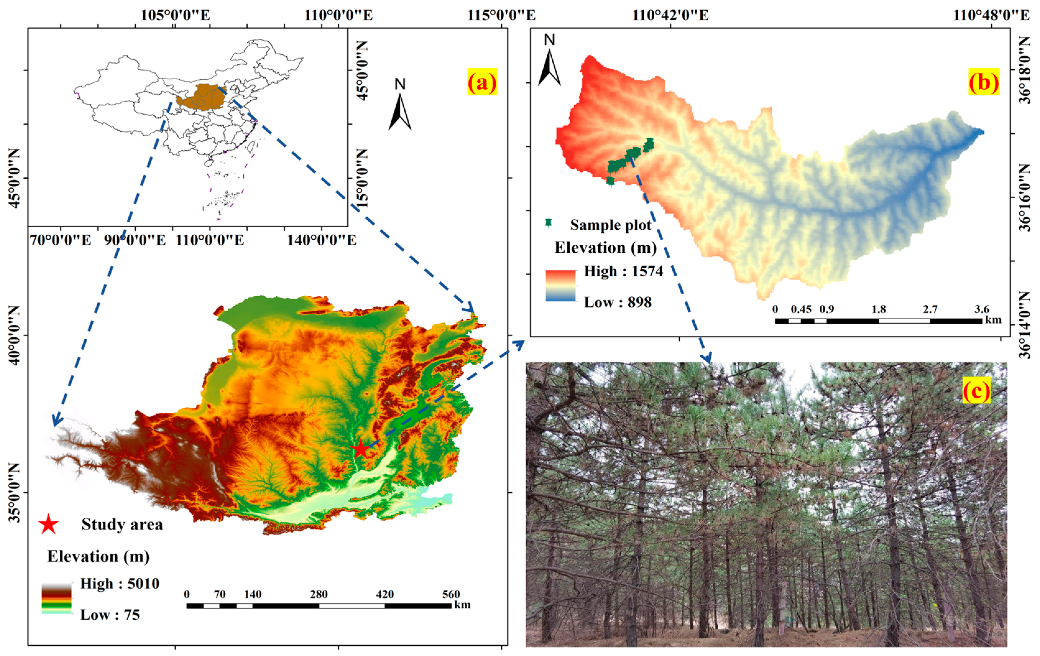
2.1. Study Area

The study area is located in the Caijiachuan watershed of Jixian County, Shanxi, in the southeastern part of the Loess Plateau. The geographic coordinates range from 110°39′45″ to 110°47′45″E and from 36°14′27″ to 36°18′23″N. The terrain is characterized by higher elevations in the west and lower elevations in the east. The watershed covers an area of 39.33 km2, with elevations ranging from 900 to 1500 m above sea level. The average annual temperature is 10.0 °C, and the average annual precipitation is 575.9 mm. Most of the rainfall occurs between July and September, accounting for approximately 80% of the total annual precipitation. The average potential evaporation each year is 1730 mm, and the annual frost-free period lasts 172 days. This area has a continental climate typical of the warm temperate zone. The soil consists of brown, loamy parent material and has a thick layer; however, it is weakly resistant to erosion due to its loose structure. The main land use types in the watershed include forest land, shrubland, grassland, and farmland, with a forest coverage rate exceeding 80%. The upper reaches of the watershed are primarily covered by natural secondary forests composed of Quercus wutaishanica, Populus davidiana, Betula dahurica, and Syringa pekinensis. The middle-upper reaches mainly consist of plantations dominated by Pinus tabuliformis, Robinia pseudoacacia, and Platycladus orientalis, while the lower reaches are characterized by grasslands and farmlands [52]. The study area is presented in Figure 1.

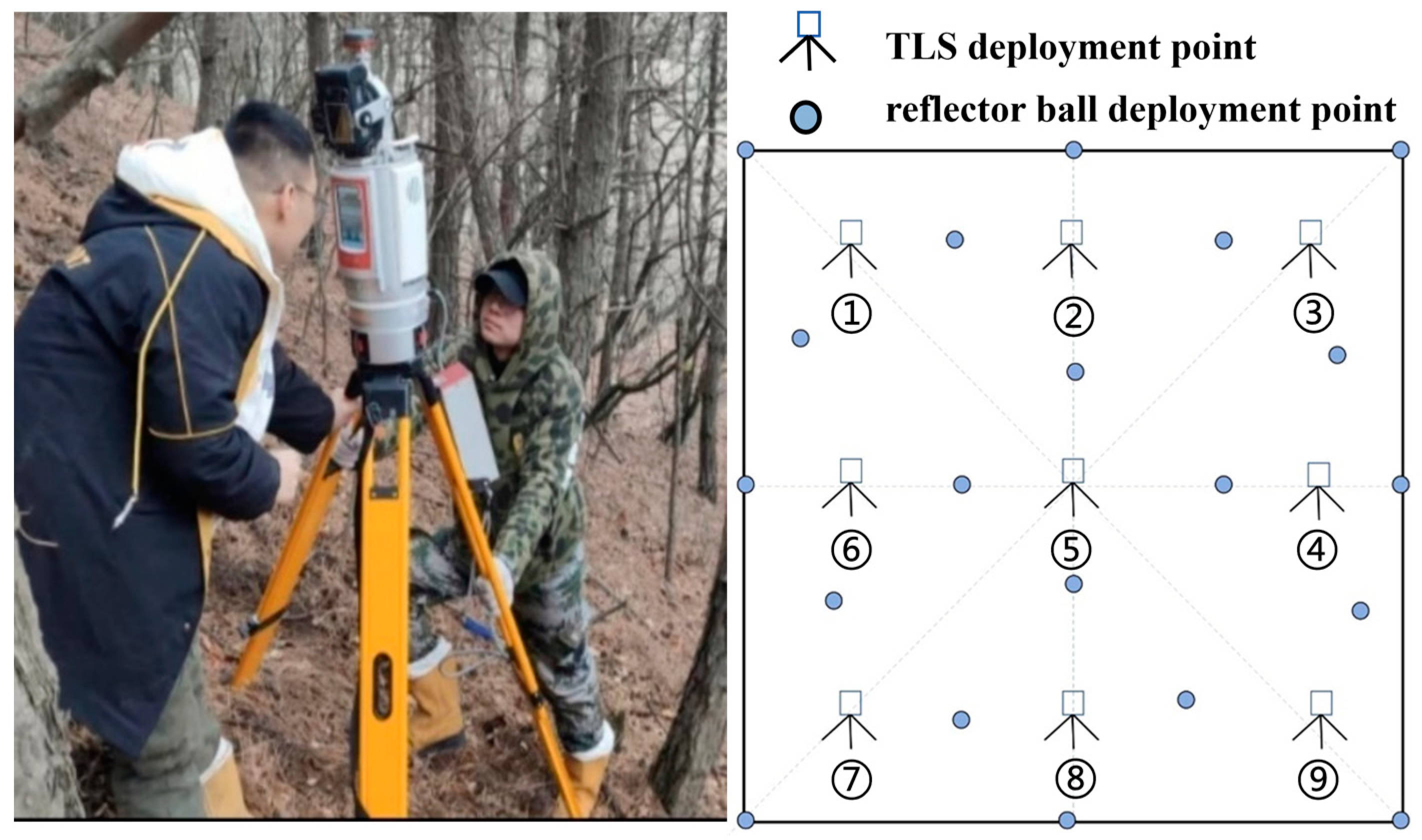
2.2. Survey Data of Sample Plots

In March 2024, 30 plantation plots of P. tabulaeformis in the Caijiachuan watershed, with a stand age of 30 years and similar stand conditions, were selected for the study. The plant density in the plots ranged from 1250 to 5900 plants per hectare. None of the sample plots contained dead or fallen trees, with a total of 3501 trees. Each tree was measured within the plots; DBH was recorded using a circumference tape, and H was calculated using the fish pole method [53]. Based on the average H and DBH measured at each site, a standard tree was selected from each location. In total, 30 standard trees were harvested, excavated, and divided into four components: leaves, branches, trunk, and roots. The fresh mass of each element was weighed and recorded (denoted as M). Subsequently, 1 kg of samples from each component was taken back to the laboratory, where the samples were placed in an oven set at 75 °C to dry until a constant weight was achieved. After drying, the dry mass of each component (denoted as m) was recorded.
The moisture content (ω) of each element was calculated using the following equation:
ω = 1 m m × 100 %
where ω represents the water content of each organ and m is the dry mass of 1 kg of each organ sampled.
The biomass (B) of each standardized wood component was then determined as
B = M ( 1 + ω )
where M indicates the fresh mass of each organ, and B refers to the biomass of each component of the standard wood.
The total biomass (BT) of standardized wood was obtained using
B T = B l + B b + B t + B r
where B T is the total biomass of the standard wood. Specifically, B l , B b , B t , and B r represent the biomass of the leaves, branches, trunk, and roots of the standard wood.
Additionally, the basic conditions of the sample plots were assessed using a geological compass and a Real-Time Kinematic (RTK) surveyor, as shown in Table 1.

2.3. Standard Tree Biomass Modeling

Developing anisotropic growth models based on the regression relationship between H, DBH, and biomass is a practical approach for estimating the biomass of individual trees and stands. Most equations for biomass anisotropic growth utilize H and DBH as separate explanatory variables or in combination [54]. Equations in the form of univariate linear, quadratic, and power functions were used to establish regression relationships. In this analysis, the H and DBH of standard trees from 30 sample plots served as explanatory variables, while biomass was the response variable. A total of 12 equations were developed, as shown in Table 2. All models were fitted using the lm() function in R 4.4.2 programming language [55].

2.4. Terrestrial Laser Scanning Data

2.4.1. Data Acquisition and Processing

To ensure temporal consistency between the TLS point cloud data and the ground-truthing data, data collection was carried out under clear, windless weather conditions in March 2024. To acquire the TLS point cloud data, 30 sample plots were scanned using the RIEGL VZ-2000i system (RIEGL Laser Measurement Systems GmbH, Horn, Austria). Table 3 presents the key performance specifications of the RIEGL VZ-2000i system.
To minimize tree occlusion during sampling, a 9-station scanning mode was used, scanning trees consecutively in a clockwise direction to collect point cloud data. Transmitter spheres were evenly placed along the plot boundaries and in unobstructed areas around the sample trees. This ensured that at least three identical transmitter spheres were visible from neighboring scan locations, facilitating the stitching of the TLS point cloud data. Figure 2 illustrates the scanning of the sample plots and the specific layout of the scanning stations. The scanning sequence follows an S-shaped pattern across three elevation levels (upper, middle, and lower slopes), with a scanning time of approximately 1–2 min per station and a total measurement time of around 20 min for the nine-station process, including the repositioning time between stations.
After data acquisition, supporting RiSCAN PRO 2.0 software registered the TLS data from the multi-station scanning into a common coordinate system, ensuring coordinate alignment with an error of less than 1 cm. This process met the accuracy requirements for forestry applications, and the stitched point cloud data were then imported into LiDAR 360 V 5.2.2 software. A detailed description of the LiDAR 360 V 5.2.2 software is provided in Appendix A.

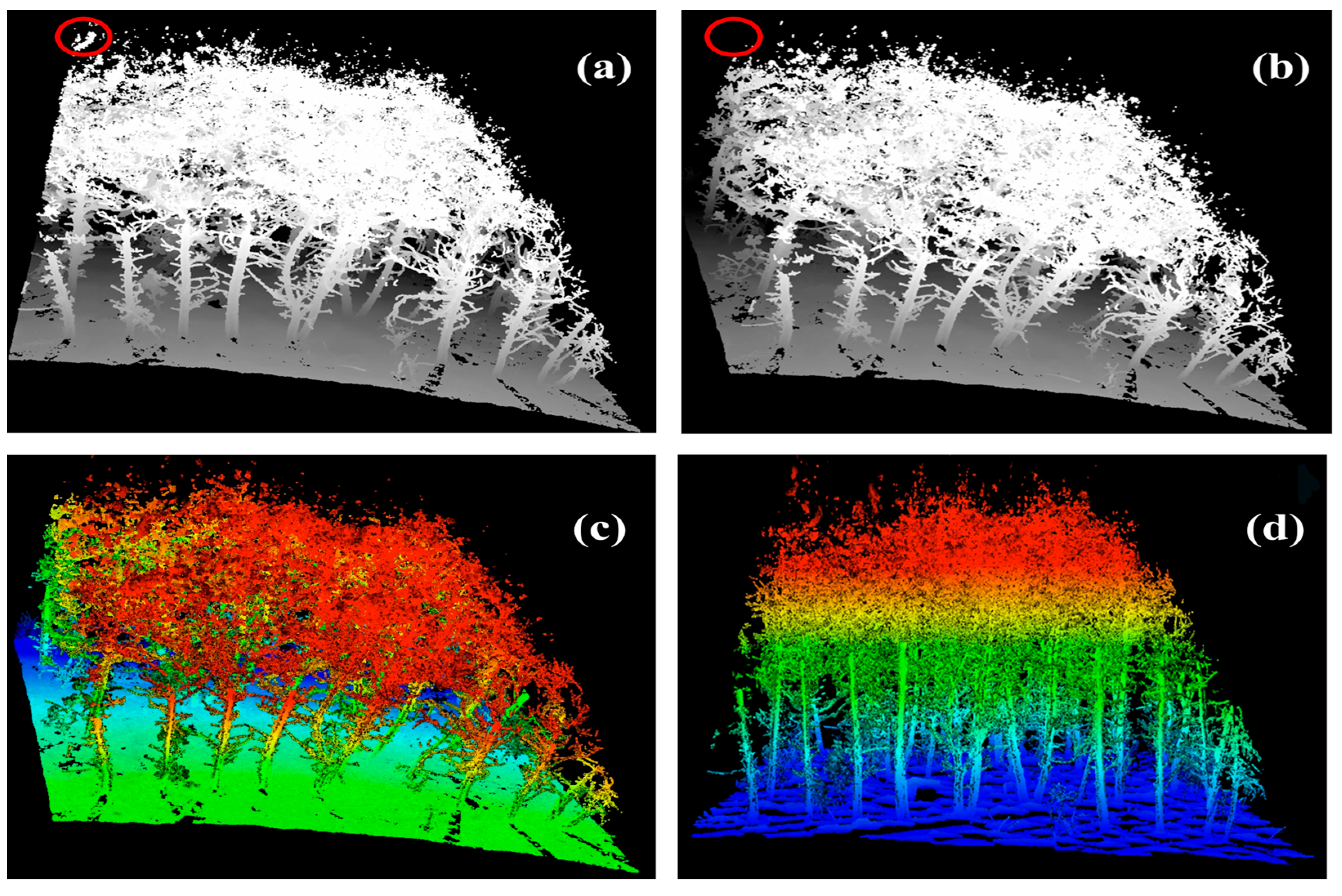
2.4.2. Pre-Processing

The neighborhood point algorithm [56] was utilized in LiDAR 360 V 5.2.2 software for the denoising process. This method examines each point to find neighboring points within a specified range. The algorithm calculates the mean distance from the point to its neighboring points and the median and standard deviation of these distances. If the mean distance of a point exceeds the maximum allowable distance—defined as the median plus a multiplier of the standard deviation—the point is classified as noisy and removed from the dataset. According to the study area, this study used 10 points as domains with a standard deviation set to 5 for denoising, as shown in Figure 3a,b.
On this basis, an improved progressive encrypted triangular mesh filtering algorithm [57] was used to classify the ground points (Figure 3c); Kriging Interpolation [58] was used to generate the digital elevation model (DEM) for the filtered ground points; and the point cloud was normalized based on the DEM to remove the influence of terrain undulation on the height of the point cloud data (Figure 3d).

2.4.3. Individual Tree Segmentation and Accuracy Evaluation

Based on the normalized processing of point cloud data, point cloud segmentation is carried out to obtain single wood point cloud data by using the direct point-cloud-oriented CSP algorithm, which is based on the principle of using the DBSCAN density-based clustering algorithm [59] for the detection of tree trunks, detecting the path distances of the crown points to reach the roots of the trunks and separating the different single wood according to the shortest path distances of the crown points to the origins of the trunks to crown points, realizing the segmentation of the crown point cloud, and, finally, realizing the overall segmentation of the point cloud of single wood (Figure 4, Appendix B).
The individual tree positions measured using RTK were compared with the positions obtained from the individual tree segmentation. A detected position was considered correct if it uniquely matched an actual measured tree. It was categorized as under-detected if multiple actual measured trees were present for that position and as over-detected if no actual measured tree could be found [60].
To evaluate the precision of individual tree segmentation, the actual count of plants in each sample plot was used as the actual value. The performance of the algorithm in segmenting trees was evaluated using three metrics: recall rate (R), precision (P), and the F-score (F) [61].
R = T P T p + F n
P = T P T p + F p
F = 2 ( R × P ) R + P
where R represents the ratio of correctly segmented plants in individual tree segmentation to the actual number of plants. P denotes the ratio of correctly segmented trees in individual tree segmentation to the total number of trees identified through the segmentation process. F is the weighted harmonic mean of R and P. Tp represents the number of correctly segmented trees. Fn represents under-segmentation, referring to the number of trees present in the actual sample plot but not successfully segmented, that is, the number of missed segments. Fp refers to over-segmentation, which indicates the number of trees that were incorrectly segmented in the actual sample plot, the number of falsely detected trees.

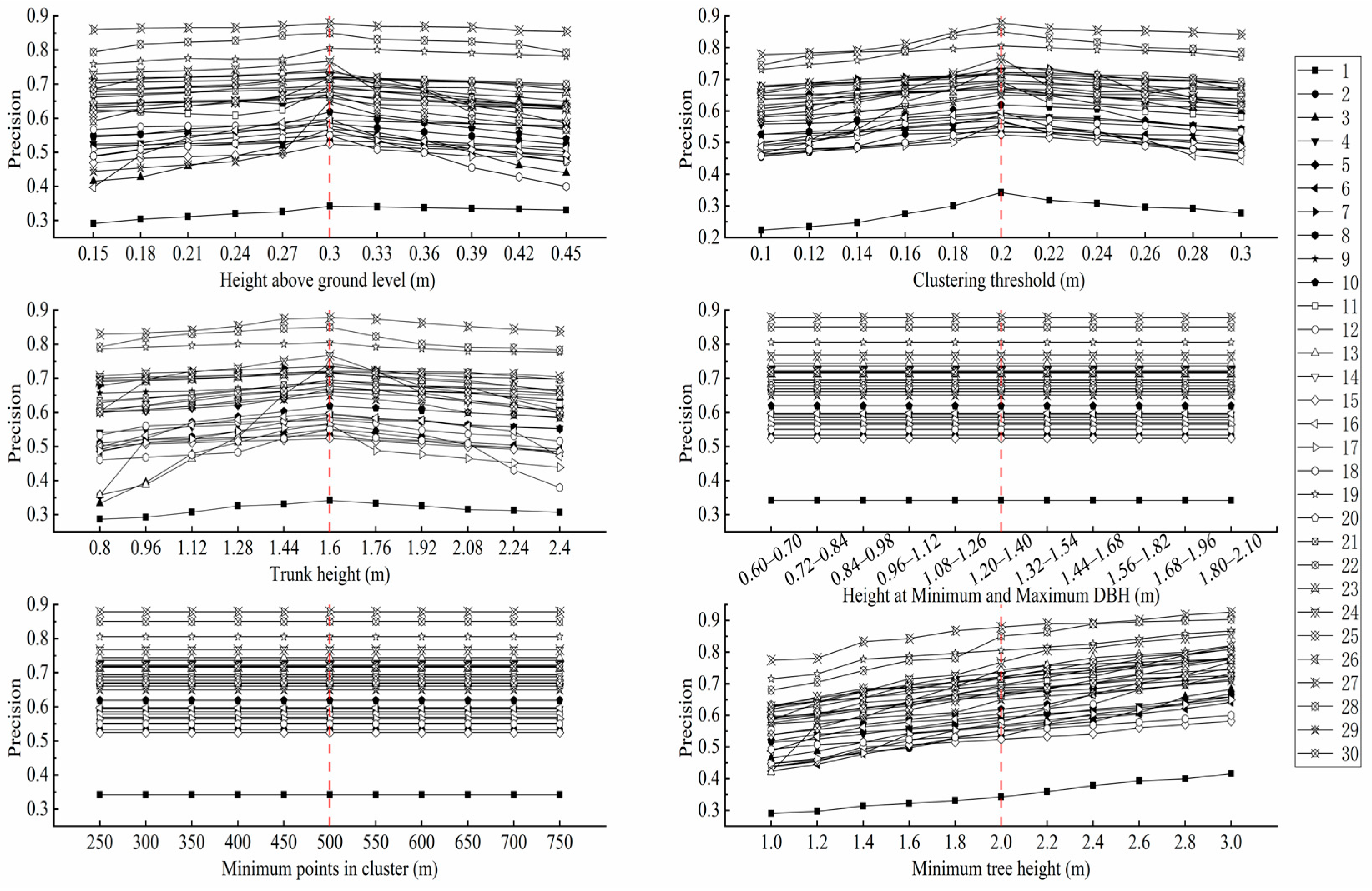
2.4.4. Sensitivity Tuning of Individual Tree Segmentation Parameters

During individual tree segmentation operations in LiDAR 360 V 5.2.2 software, the parameter settings included height above ground level, clustering threshold, trunk height, height at minimum and maximum DBH, the minimum points in the cluster, and minimum tree height, and the above parameters were independently gradient adjusted within the range of 0.5–1.5 times the system default values, with only a single parameter being changed at a time and the rest of the parameters remaining at the system default values. The precision of the segmentation results was calculated using Equation (5) to analyze the effect of each parameter variation on individual tree segmentation (Figure 5). Under the default parameter settings of the system, height above ground level, clustering thresholds, and trunk height have the highest accuracy rates and the best segmentation results. The precision remained constant as height at the minimum and maximum DBH and the minimum number points of the cluster were varied. As the minimum tree height varied, the precision also exhibited a corresponding trend of change.
Accordingly, the parameters were set as follows: above ground level at 0.3 m, clustering threshold at 0.2 m, trunk height at 1.6 m, minimum DBH height at 1.2 m, maximum DBH height at 1.4 m, and the minimum number points of in cluster at 500. The minimum tree height was determined based on the actual growth conditions of the local tree population.
According to the minimum tree height data from the field survey of the sample plots (Figure 6), the minimum tree heights of the 30 sample plots in this study area ranged from 3.0 to 5.5 m. Therefore, six groups of minimum tree heights of 3.0, 3.5, 4.0, 4.5, 5.0, and 5.5 m were set up in sequence for point cloud segmentation in this study.
By comparing the segmentation results with the actual conditions of the sample plots, the optimal minimum tree height setting for point cloud segmentation in the study area was analyzed. This optimization aimed to improve the accuracy of individual tree segmentation and the subsequent extraction of stand parameters, providing a new technical approach for forest resource investigations in the region.

2.4.5. Stand Parameter Extraction and Accuracy Evaluation

Point cloud slices with a thickness of 5 cm (ranging from 1.27 to 1.32 m) were extracted from the segmented point cloud data to obtain the individual tree DBH using the least squares circle fitting method [62]. After normalization, the height of the ground point in the point cloud is set to 0 m. The z-coordinate of the highest point of an individual tree is then extracted to determine the vertical elevation of the tree [63]. Please refer to Appendix B for details. Equation (7) was utilized to calculate the extraction accuracy (φ) of the stand parameters across various sites.
The measured values of the stand parameters for each sample site were used as the control, and the coefficient of determination (R2) was calculated using Equation (8). This coefficient tests the goodness-of-fit of the regression line, with larger values of R2 indicating a stronger correlation between the dependent and independent variables. Equation (9) is used to calculate the root mean square error (RMSE) between the actual and predicted values. A smaller RMSE indicates better prediction accuracy [64]. The specific formula is as follows:
φ = 1 1 n i = 1 n T i P i T i
where n is the number of correctly separated stands; Ti is the estimated value of the separated stand parameters; and Pi is the measured value corresponding to the separated stand parameters.
The measured values of the stand parameters for each sample site were used as the control, and the coefficient of determination (R2) was calculated using Equation (8). This coefficient tests the goodness-of-fit of the regression line, with larger values of R2 indicating a stronger correlation between the dependent and independent variables.
R 2 = 1 i = 1 n ( T i P i ) 2 i = 1 n ( P i P ¯ ) 2
where n is the number of correctly separated stands; Ti is the estimated value of the separated stand parameters; and Pi is the measured value corresponding to the separated stand parameters. P ¯ is the arithmetic mean of the measured values corresponding to the separated stand parameters.
Equation (9) is used to calculate the root mean square error (RMSE) between the actual and predicted values. A smaller RMSE indicates better prediction accuracy. The specific formula is as follows:
R M S E = i = 1 n ( T i P i ) 2 n 1
where n is the number of correctly separated stands; Ti is the estimated value of the separated stand parameters; and Pi is the measured value corresponding to the separated stand parameters.

3. Results

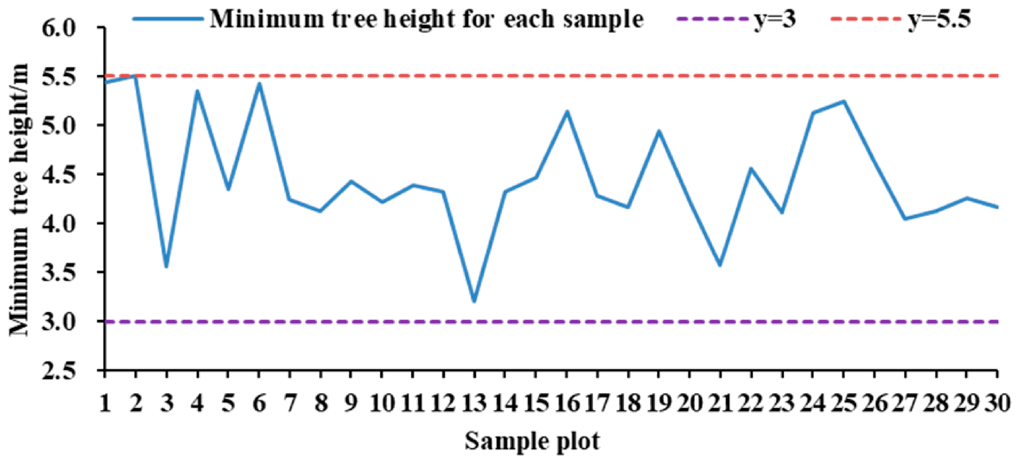
3.1. Accuracy of Individual Tree Segmentation

By comparing the segmented TLS point cloud data with the field-measured data, the results of individual tree segmentation and accuracy for six sets of minimum tree height settings (3, 3.5, 4, 4.5, 5, and 5.5 m) are shown in Table 4. For the sets with minimum tree heights of 3, 3.5, and 4 m, the total number of identified trees was 3920, 3727, and 3556, respectively, which is significantly over-segmented compared to the field-measured total of 3501 trees. In contrast, for the sets with minimum tree heights of 4.5, 5, and 5.5 m, the total number of identified trees was 3406, 3261, and 3114, respectively, which shows a clear under-segmentation compared to the measured values. The R decreases as the minimum tree height increases, while the P increases with the height. According to the F, the highest individual tree segmentation accuracy of 0.9475 is achieved when the minimum tree height is set to 4.5 m.

3.2. Assessing the Accuracy of Diameter at Breast Height Extraction

The results for the extraction accuracy of the average DBH for each sample plot obtained through TLS are presented in Table 5. Across the 30 sample plots divided into six groups, with minimum tree heights set at 3, 3.5, 4, 4.5, 5, and 5.5 m, the average extraction accuracy was consistently above 0.9247. This indicates that the extraction accuracy of the average DBH for the sample plots using TLS is generally high. The lowest average extraction accuracy recorded was 0.9247 for the shortest tree height of 3 m, while the highest accuracy was 0.9677 for the minimum tree height of 5 m.
The results of the linear fit between the extracted and measured values of the mean breast diameter at the minimum tree height of 5 m are shown in Figure 7a, with R2 of 0.9275 and RMSE of 0.3916 cm, which is less than 0.5 cm in general, indicating that the extracted DBH of an individual tree correlates well with the measured values when the minimum tree height is set at 5 m. The variation in extraction accuracy of DBH exhibited a general trend of initially increasing (7.5430–8.4922 cm) and then decreasing (8.4922–14.0880 cm) as the average DBH increased. The average DBH for each sample site ranged from 7.5430 to 14.0880 cm for extracted values and from 7.5140 to 14.5120 cm for measured values.
As shown in Figure 7b, approximately 63% (19 sample plots) of the extracted mean diameter at breast height (DBH) values were underestimated compared to the measured values, while 37% (11 sample plots) were overestimated.

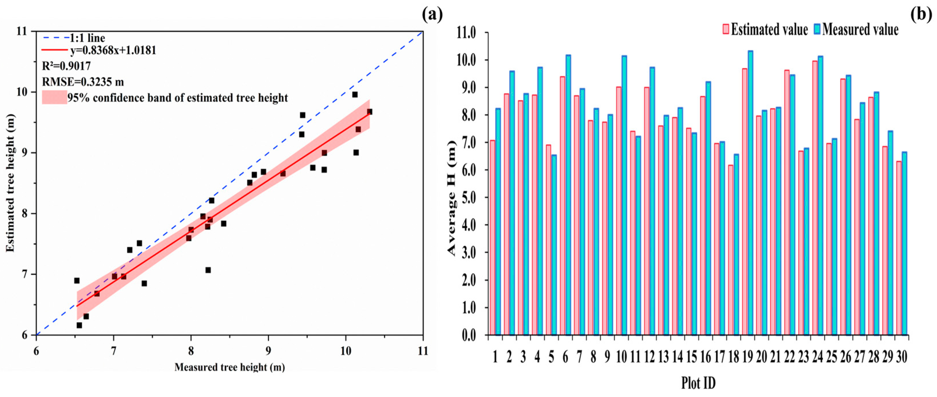
3.3. Assessing the Accuracy of Tree Height Extraction

The results of the average H extraction accuracy of each sample plot using TLS are shown in Table 6, and the average extraction accuracy of all sample plots reached more than 0.8791, which indicates that while the accuracy of H extraction based on TLS is lower than that of DBH extraction, the performance of H estimation remains satisfactory. The groups with the lowest and highest extraction precision were the same as those for DBH; the group with the shortest tree height of 3 m (0.8791) and the group with the shortest tree height of 5 m (0.9518), respectively.
The linear fitting results based on the average H extracted values and measured values at the minimum tree height of 5 m are shown in Figure 8a, with R2 of 0.9017 and RMSE of 0.3235 m, which is less than 0.5 m in general, indicating that the average H extracted values of the sampled plots still correlate well with the measured values when the minimum tree height is set to 5 m. The accuracy of H extraction gradually decreased as the average H increased. The extracted mean H values for each sample site ranged from 6.1613 to 9.9593 m, while the measured values ranged from 6.5248 to 10.3091 m.
Figure 8b shows that the extracted values of the average tree height of each sample site were underestimated in about 87% (26 sample sites) and overestimated in about 13% (4 sample sites) of cases compared to the measured values.

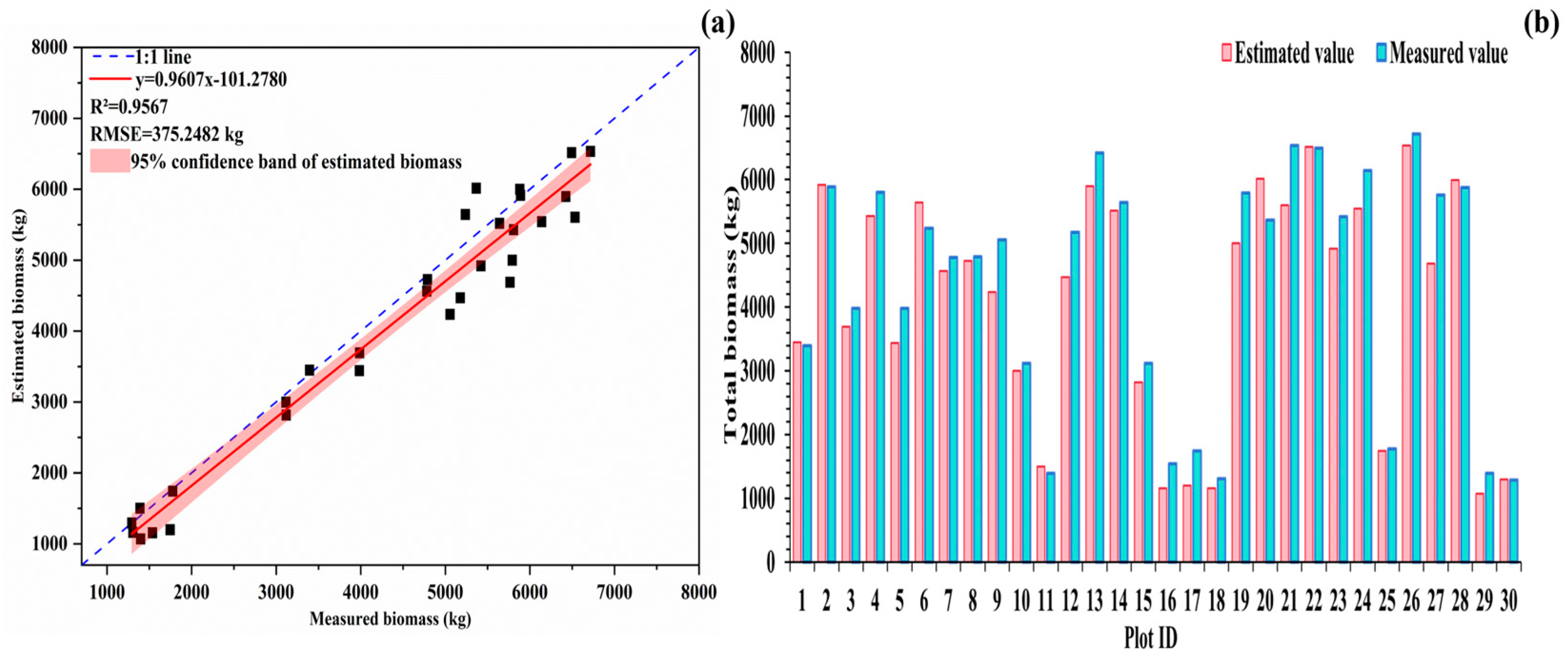
3.4. Biomass Modeling and Accuracy Evaluation

Regression relationships between standard tree biomass, H, and DBH were developed for 30 sample plots. Calculation of R2 and RMSE values for logarithmic, univariate linear, multivariate linear, and power functions allowed for the selection of the best equation form (Table 7). The equation B = a ( D 3 H ) b produced the best R2 value of 0.9141 and the smallest RMSE of 8.8055 kg. The biomass estimation model that performed the best was B = 0.927 ( D 3 H ) 0.7327 , which was determined by combining the R2 and RMSE values.
Table 8 shows the precision of total biomass estimation for each sample site. The average precision across all six groups exceeded 0.8794, indicating that the precision of total biomass estimation was generally high for each sample site. The lowest precision was observed in the shortest tree height 3 m group, with a value of 0.8794, while the highest precision was found in the shortest tree height 4.5 m group, with a value of 0.9066.
Figure 9a shows the linear fitting results between the estimated and measured total biomass for each sample site at the minimum tree height of 4.5 m, with an R2 of 0.9567 and an RMSE of 375.2482 kg, indicating a strong correlation between the estimated and measured values. The estimated total biomass for each sample site ranged from 985.7 to 6566.4 kg, while the measured values ranged from 1290.7 to 6715.6 kg.
As illustrated in Figure 9b, 73% (22 plots) of the total biomass estimates were lower than the actual values, while 27% (8 plots) were higher than the actual values.

4. Discussion

4.1. Analysis of the Accuracy of Diameter at Breast Height Extraction

Currently, Hough transform [65,66], the RANSAC algorithm [67], the ensemble deep convolutional neural network [68], and the least squares circle fitting method [69] are often used to extract the diameter of the chest, etc. Hough transform usually needs to rasterize the data first, and this process may lead to the loss of detailed information [70]. The RANSAC algorithm in the complicated environment has strong robustness to noise and anomalies, but its computational complexity is high, and the number of iterations rises significantly with the increase in data complexity and noise level, resulting in low computational efficiency [71]. Ensemble deep convolutional neural networks can achieve higher estimation accuracy through deep feature fusion, but they usually require a large amount of labeled data, complex network design, and higher computational resources, and they are more sensitive to hyperparameters [72]. In contrast, the least squares circle fitting method directly uses the point cloud data for fitting without rasterization, so it can retain more detailed information, and, at the same time, in the complex iterative process of the RANSAC algorithm, the least squares circle fitting method can quickly converge to the optimal solution, so it has high computational efficiency in most cases [73].
Approximately 63% of the sample plots in this study yielded underestimated mean chest diameter values, while 37% showed overestimated values compared to the actual measurements. The main reason for the underestimation of DBH is likely to be due to the point cloud data collection process. Trees with smaller DBH have fewer point cloud points due to their smaller cross-sectional area, resulting in insufficient feature support for the fitted model. This lack of data contributes to the underestimation of DBH, which is particularly pronounced in dense forest stands or complex terrain. Additionally, the least squares circle fitting method assumes a circular cross-section. However, in practice, the trunk cross-section may deviate from the ideal shape due to factors like tree species characteristics, the growing environment, and other influences. Trees with either very small or huge DBH may lead to underestimation [74].
The overestimation of DBH in individual samples may be due to certain scanning angles where neighboring scaly epidermal layers shadow each other, creating an artifact in the scan data that appears as a “bulge” in some areas of the trunk, leading to extracted DBH values higher than the actual measured values.

4.2. Analysis of the Accuracy of Tree Height Extraction

Errors in H extraction mainly stem from trunk point cloud quality and forest type [75]. Multi-station scanning (nine sites in this study) improved data coverage and reduced occlusion errors, achieving an accuracy of up to 0.9677, outperforming single-station results in previous studies [76].
Forest complexity also affects accuracy [77]. Our results were higher than those in tropical rainforests [78], likely due to the simpler forest structure and minimal understory vegetation at our site. Compared to broadleaf forests, where canopy overlap and self-shading hinder H extraction, our method performed better [79].
The extracted mean H values for each sample in this study were underestimated in approximately 87% of the sample plots (26 plots) and overestimated in about 13% (4 plots) compared to the true values, which aligns with the findings of previous studies [80,81]. Because TLS operates from the bottom–up, dense upper canopy layers may cause the laser to be reflected multiple times as it passes through, preventing some of the laser pulses from reaching the top of the tree. Such conditions can result in point cloud data not covering the highest points, leading to an underestimation of H.

4.3. Analysis of the Accuracy of Biomass Estimation

In this study, the average biomass estimation accuracies of each site under the six groups of minimum tree height parameter settings reached more than 0.8794, with the highest accuracy of 0.9066 in the 4.5 m minimum tree height group. Compared to the QSM model of Dong et al. [82], the TLS-based biomass estimation method of the present study demonstrated higher accuracies in evergreen coniferous forests. This may be due to the fact that although QSM can construct detailed 3D tree structure models to improve the accuracy of biomass estimation, it is more applicable to mature deciduous trees and usually works best under leaf shedding conditions [83,84]. For evergreen coniferous forests, especially creosote pine forests, the QSM method has challenges in removing needle point clouds, resulting in limited biomass estimation accuracy [85]. Although the TLS-based method in this study outperformed QSM in terms of accuracy, QSM still has a unique advantage in 3D tree structure modeling. Future studies may consider combining the TLS and QSM methods in order to fully utilize the high-precision point cloud data of TLS and at the same time conduct detailed tree structure analysis with the help of QSM modeling to achieve more accurate biomass estimation. In addition, the introduction of multi-scale fusion methods may help to improve modeling accuracy under heterogeneous forest structures and make biomass estimation more stable and reliable.
Biomass estimates were underestimated in 73% (22 samples) and overestimated in 27% (8 samples) of cases compared to the actual values. The underestimation may be attributed to the fact that most samples had underestimated DBH and H, which likely led to biomass estimates based on DBH and H also being underestimated.

4.4. Correlation Analysis of Factors Affecting Biomass

In this study, the highest precision of individual tree segmentation was in the group with the minimum tree height of 4.5 m, the highest precision of DBH extraction was in the group with the minimum tree height of 5 m, the highest precision of H extraction was in the group with the minimum tree height of 5 m, and the highest precision of sample plot biomass extraction was in the group with the minimum tree height of 4.5 m.
According to the correlation analysis in Table 9, a highly significant positive correlation was found between individual tree biomass and both DBH and H, with DBH showing a stronger correlation than H, which is consistent with the findings of Zhao et al. [85]. Tree DBH is closely related to the volume of internal xylem and biological tissues, which not only provide structural support to the tree but also play a critical role in biomass accumulation and significantly influence biomass composition. In contrast, while an increase in H also contributes to biomass growth, its impact is relatively minor in magnitude [86].
Sample-scale biomass, plant number, DBH, and H all showed a highly significant positive correlation. However, the factors differed from single-tree-scale biomass, with the degree of impact following the order single-tree plant number > H> DBH. The influence of single-tree plant number was more significant than that of DBH and H. This may be because accurate tree segmentation is fundamental to biomass estimation, and inaccuracies in individual tree segmentation affect the extraction of DBH and H data, further increasing the error in biomass estimation [87]. This explains why tree height and DBH exhibited the highest precision at a minimum tree height of 5 m, while biomass estimation and individual tree segmentation achieved the highest precision at a minimum tree height of 4.5 m. The highest precision for tree height and DBH was attained at a minimum tree height of 4.5 m.
H had a greater influence on sample-scale biomass than DBH, which differs from the findings of Li et al. [88]. This discrepancy may be attributed to the fact that the minimum tree heights measured across several sample plots ranged from 3 to 5.5 m. As the minimum tree height for individual tree segmentation increased, the distribution of trees in some sample plots likely became more concentrated on those with larger DBH and more mature individuals, thereby reducing the influence of diameter at breast height on biomass estimation. As the minimum tree height increased, the biomass distribution of the tree changed; the proportion of biomass in the crown portion (e.g., leaves and branches) increased, while the proportion in the trunk portion relatively decreased, thus highlighting the importance of tree height in biomass accumulation [89].

4.5. Research Limitations and Future Prospects

In this study, the neighborhood point algorithm in LiDAR 360 V 5.2.2 software is used for denoising, which removes isolated noise based on neighborhood statistical features and achieves better denoising results under the conditions of the study area. However, the definition of noise points in this method depends on preset parameters (e.g., neighborhood size and standard deviation multiplicity), and the generalization ability in different datasets still needs to be further verified. In addition, the method mainly targets outlier denoising and may have some limitations for more complex noise patterns (e.g., dense background noise or dynamic noise) [90]. In recent years, some more advanced denoising methods, such as sharpness assessment methods combining time–frequency domain analysis (e.g., wavelet transform, Fourier transform), have been proposed, which are able to retain the edge and structural information of the point cloud more efficiently in the denoising process and improve data quality. Meanwhile, lightweight multi-target detection algorithms (e.g., optimized YOLO variants) can also be used for subsequent point cloud target identification to enhance the applicability of the data [91]. Future research can combine deep learning methods (e.g., PointNet, SparseCNN) and time–frequency domain sharpness assessment to optimize the denoising strategy for point cloud data in order to further improve the processing accuracy and generalization capability.
In point cloud segmentation, self-attention mechanisms, which can adaptively capture long-range dependencies between different regions, have achieved significant results in tasks like scene classification and object detection in recent years [92]. By strengthening the correlation between local and global features, self-attention mechanisms can enhance the model’s understanding of complex scenes, which is expected to improve the accuracy of individual tree segmentation [93]. In the future, it is planned to combine the self-attention mechanism with existing segmentation algorithms to further validate its application in single-tree segmentation, especially when dealing with complex relationships between trees in dense forest stands.
In recent years, multi-layer fusion network (MLFN) methods have made some progress in addressing errors caused by complex tree canopy occlusion. These methods mainly rely on (1) multi-scale feature extraction, capturing both local and global information to compensate for the lost structural details in occluded regions; (2) hierarchical feature fusion, combining shallow high-resolution features and deep semantic information to improve the resolution of complex occluded areas; and (3) enhancement of model robustness, enabling the model to maintain high accuracy in the presence of noise and occlusion [94]. Although multi-layer fusion networks show potential in remote sensing imagery and point cloud processing, their application in forest stand parameter estimation still faces challenges, such as the high demand for high-quality labeled data and high computational resource consumption [95]. Future research could try to combine multi-layer fusion network methods with traditional rule-based segmentation algorithms, such as using deep learning methods for occlusion region compensation and optimizing them with lightweight algorithms like CSP, in order to strike a balance between computational efficiency and accuracy. At the same time, future research should focus on improving the resolution and quality of point cloud data acquisition. In terms of data collection, using more accurate laser scanning equipment can significantly enhance point cloud coverage, reducing the risk of underestimation. Regarding algorithms, incorporating dynamic fitting techniques, such as elliptical or other more adaptive models, can help reduce the bias introduced by cross-sectional assumptions.
As shown in Figure 10, the biomass inversion results of this study were limited to 30 sample plots and could not cover the entire Caijiachuan watershed. Due to limitations in data acquisition and research methodology, biomass data could only be interpolated based on the measurements from these 30 sample plots, generating biomass distribution maps for local areas. Large-scale biomass inversion across the entire watershed was not feasible. The absence of remote sensing data (e.g., unmanned aerial LiDAR, aerial LiDAR, or high-resolution satellite imagery) covering the whole watershed is a key limitation of this study. Future research should combine large-scale remote sensing data with advanced modeling techniques (such as data extrapolation or remote-sensing-based biomass estimation models) to expand the spatial coverage of biomass inversion and enhance the accuracy and reliability of the results.
Furthermore, the Caijiachuan watershed encompasses various land use types. The current allometric growth model for P. tabuliformis biomass is based solely on standard logging measurements and lacks empirical data for other vegetation types. While relevant allometric growth models exist, their limited validation data restrict their broader application. Future studies should focus on collecting and validating biomass equations for different vegetation types to improve the accuracy and applicability of biomass estimation.
Finally, relying solely on terrestrial laser scanning technology presents challenges in accurately estimating biomass at the watershed scale. Given the absence of biomass equations applicable to all vegetation types, this study was confined to analyses within the available sample plot data. Combining remote sensing and terrestrial laser scanning techniques in future research will help improve the accuracy and reliability of biomass inversion at the watershed scale.

5. Conclusions

The artificial P. tabuliformis forest planted in the Caijiachuan watershed of Jixian County, Shanxi, located in the southeastern part of the Loess Plateau, was selected as the research subject. TLS was used for remote sensing image acquisition, and CSP algorithms were applied for individual tree segmentation, enabling the rapid and accurate extraction of stand parameters (DBH and H) and precise biomass.
By comparing the TLS data after individual tree segmentation with the measured data, R decreases as the minimum tree height increases, while P increases with the minimum tree height. According to the F, the highest individual tree segmentation precision of 0.9475 is achieved when the minimum tree height is set to 4.5 m.
Overall, the accuracy of H and DBH, as well as biomass estimation using TLS, was high in this study. The average accuracies for DBH and H extraction and biomass estimation across 30 sample plots in six groups with minimum tree heights of 3, 3.5, 4, 4.5, 5, and 5.5 m were all above 0.9247, 0.8791, and 0.8794, respectively. When the minimum tree height was set to 5.0 m, the highest extraction accuracies for DBH and H were achieved, with values of 0.9677 and 0.9518, respectively. According to the linear fitting results between the extracted and measured values, the R2 for average DBH was 0.9275, and the RMSE was 0.3916 cm. The average H had an R2 of 0.9017 and an RMSE of 0.3235 m. The highest biomass estimation accuracy of 0.9066 was achieved when the minimum tree height was set to 4.5 m. Based on the linear fitting of the extracted values to the measured values, R2 was 0.9567, and RMSE was 375.2482 kg.
This study offers a fast and efficient technical approach for forest resource surveys in the Loess Plateau region. The next step will be to further optimize the algorithms and explore the integration of multi-source data to provide reliable support for forest resource management in the Loess Plateau region. Further research will focus on refining algorithmic efficiency to enhance classification accuracy and computational performance while integrating diverse data sources—including UAV imagery, satellite optical, and radar data—to improve monitoring precision. Additionally, future studies will emphasize validating the proposed approach across various ecological regions, ensuring its robustness and scalability. Efforts will also be directed toward facilitating its practical implementation in forest resource management, contributing to more effective and data-driven decision making for sustainable environmental conservation.

Author Contributions

Conceptualization, M.H.; methodology, M.H. and Y.H.; software, M.H., Y.H. and Y.L.; validation, M.H., Y.H. and J.Z. (Jiongchang Zhao); formal analysis, M.H.; investigation, M.H., Y.H. and B.W.; resources, M.H. and Y.H.; data curation, M.H.; writing—original draft preparation, M.H.; writing—review and editing, M.H., J.Z. (Jiongchang Zhao), Y.H. and Y.L.; visualization, M.H., Y.H., Y.L., J.Z. (Jiongchang Zhao) and H.N.; project administration, J.Z. (Jianjun Zhang); funding acquisition, J.Z. (Jianjun Zhang) and H.N. All authors have read and agreed to the published version of the manuscript.

Funding

This research was funded by the National Key R&D Program of China, grant No. 2022YFE0104700.

Data Availability Statement

The original contributions presented in the study are included in the article; further inquiries can be directed to the corresponding author.

Acknowledgments

In addition, we thank Elsevier Publishing for granting a license for Figure A2 in Appendix B and permitting its use in this study, and we also thank the reviewers for their useful comments and suggestions.

Conflicts of Interest

Author Hidenobu Noguchi was employed by the company Asia Air Survey Co., Ltd. The remaining authors declare that the research was conducted in the absence of any commercial or financial relationships that could be construed as a potential conflict of interest.

Appendix A. Introduction to LiDAR360 V 5.2.2 Software

LiDAR360 V 5.2.2 is a powerful professional LiDAR data processing software developed by GreenValley International widely used in forest resource surveys, topographic mapping, smart city construction, power line inspection, and other fields. The software integrates a full set of functions for point cloud preprocessing, classification, modeling, and analysis, enabling efficient processing and analysis of large-scale LiDAR data. LiDAR360 V 5.2.2 supports various common data formats, such as LAS, LAZ, TXT, and PLY, and features parallel computing and automated batch processing capabilities, significantly improving the efficiency of large-scale data processing.
In terms of point cloud processing, LiDAR360 V 5.2.2 utilizes advanced algorithms for ground point extraction and point cloud classification, supporting individual tree segmentation, tree height, and diameter at breast height (DBH) extraction for forest parameter analysis. It can also calculate tree canopy features, including tree crown width, canopy depth, and more, helping to analyze the structure and health of forests. Additionally, the software uses Kriging Interpolation to generate high-precision digital elevation models (DEM) and digital surface models (DSM), providing accurate data support for topographic analysis.
LiDAR360 V 5.2.2 is also widely used in power line inspection and 3D building modeling. It can automatically extract power lines, towers, and cable sag curves and perform accurate analysis of power facilities. In urban modeling, LiDAR360 V 5.2.2 supports 3D building modeling, providing detailed cityscape reconstruction particularly suitable for digital twin and smart city development. Through its comprehensive point cloud processing and analysis capabilities, LiDAR360 V 5.2.2 offers a complete and precise data processing solution to meet the needs of various industries [96].
You can visit the official LiDAR360 V 5.2.2 website for more information and feature-related instructions: https://www.greenvalleyintl.com, accessed on 1 January 2024.

Appendix B. Detailed Methodology for Individual Tree Segmentation and Parameter Extraction

Appendix B.1. Denoising

In Lidar360 V 5.2.2, the denoising algorithm uses two key parameters: the number of neighborhood points and the standard deviation multiplier to identify and remove noise points. First, the number of neighborhood points (the default is 10) determines the range for calculating the neighboring points of each point. The algorithm selects a certain number of neighboring points (the default is 10) around each point and calculates the average distance (D) from these points to the given point. Then, the global average distance (mean D) is calculated based on the average distances of all points. If a point does not have enough neighboring points to perform the calculation, it will be skipped and not involved in the denoising process. Next, the standard deviation multiplier (the default is five) is a factor that controls the strictness of noise point identification. The algorithm compares the average distance D of each point with the global average distance (mean D) [97]. If the average distance of a point is greater than mean D×mean K (where mean K is the standard deviation multiplier), that point is considered a noise point. The smaller the standard deviation multiplier, the stricter the algorithm, and more points will be identified as noise; conversely, fewer points will be regarded as noise. Therefore, adjusting these two parameters helps users fine-tune the denoising effect according to the actual data. For this study, we used 10 neighborhood points and a standard deviation multiplier of five for denoising, as shown in Figure 3a,b.

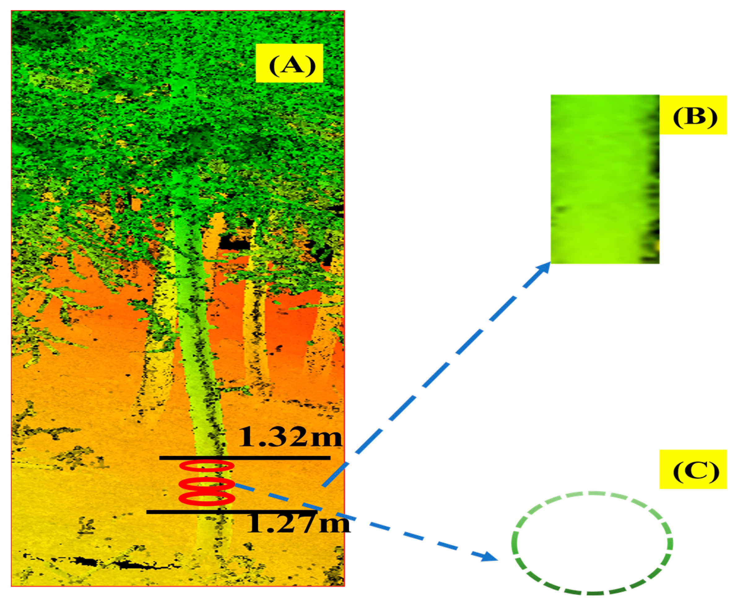
Appendix B.2. Ground Point Classification

In Lidar360 V 5.2.2, ground point classification after denoising is performed using the improved progressive triangulated mesh filtering algorithm [57], as shown in Figure 3c. The input data can be a single point cloud file or a point cloud dataset. The initial and target classes specify the points to be classified and the target class after classification, respectively. The number of points (the default is one) controls whether the classification is based on individual low points or low point clusters. The radius (the default value is 5 m) defines the distance threshold between the points to be classified and neighboring points. Neighboring points within this range will participate in the classification. The height (the default value is 0.5 m) sets the elevation difference threshold between the points to be classified and neighboring points. If the elevation difference exceeds this value, the point will be considered a non-ground point.

Appendix B.3. DEM Generation and Point Cloud Normalization

In LiDAR360 V 5.2.2 software, the “Kriging Interpolation” method is selected in the DEM generation module, and parameters are set according to research requirements [58]. The default parameters chosen for this study include a grid resolution of 0.5 m to ensure high accuracy of the DEM. The variogram model is set to Exponential, which is suitable for the terrain characteristics of the study area; the search radius is set to 30 m to balance computational efficiency and interpolation accuracy; the number of neighboring points is set to 20 to ensure sufficient data support for the interpolation calculation; the minimum number of points is set to five; and the maximum number of points is set to 50 to ensure computational stability. After setting the parameters, Kriging Interpolation is run to calculate the DEM, and the DEM file is exported (supporting GeoTIFF, ASC, and IMG formats) for subsequent point cloud normalization and terrain modeling analysis. The point cloud is normalized based on the DEM to eliminate the influence of terrain undulations on the point cloud data’s height (Figure 3d).

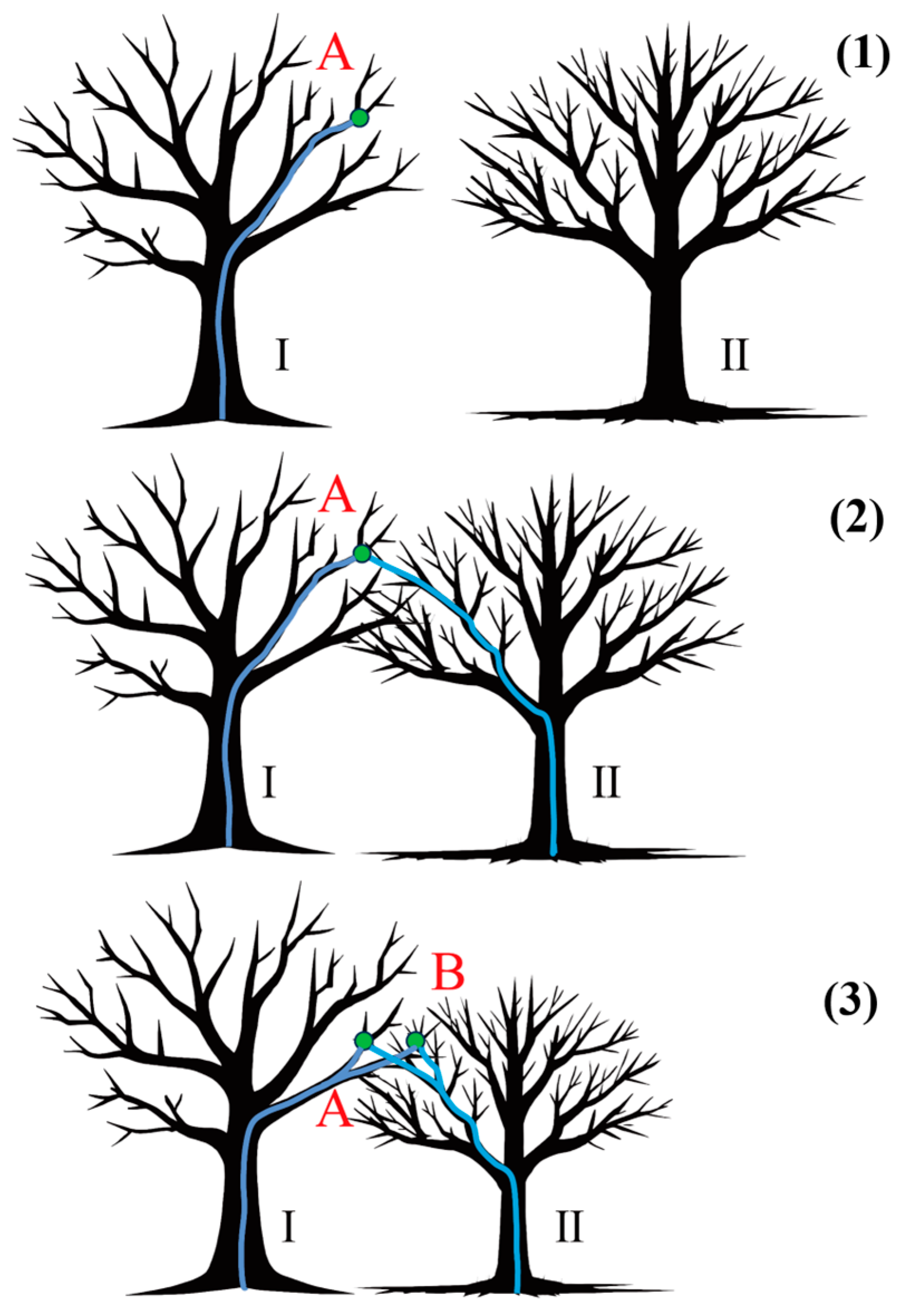
Appendix B.4. Point Cloud Segmentation Using the Comparison of Shortest Paths Algorithm

After the point cloud data are normalized, the Comparison of Shortest Paths (CSP) [42] algorithm is applied directly to the point cloud for segmentation, enabling the extraction of individual tree point cloud data. The principle of this method is as follows. First, the DBSCAN (Density-Based Spatial Clustering of Applications with Noise) [56] algorithm is used to detect tree trunks. This algorithm performs clustering analysis on point cloud data based on two key parameters: neighborhood radius (ϵ) and minimum number of neighboring points (MinPts)
During the detection process, DBSCAN identifies high-density regions in the point cloud data and clusters points with similar spatial distribution characteristics into the same category. Because tree trunks typically exhibit a continuous and densely distributed point cloud structure, an appropriate selection of ϵ and MinPts allows for distinguishing trunk points from non-trunk points (such as tree canopies and branches), as shown in Figure A1.
Figure A1. Trunk detection using DBSCAN. The red circles represent the detection of the tree trunk.
Remotesensing 17 01228 g0a1
Then, we further calculate the path distance from the crown point to the root of the main trunk. By comparing the shortest path distance from the crown point to the root of the main trunk, the crown points of different single trees can be effectively separated, which in turn realizes the segmentation of the crown point cloud and ultimately achieves the overall segmentation of the point cloud of a single tree (as shown in Figure 4).
The Comparison of Shortest Paths (CSP) algorithm is an innovative point cloud segmentation method that is particularly suitable for complex stand environments with intersecting tree canopies. The algorithm utilizes the biological properties of trees’ vascular bundle structure, combined with the shortest path principle, to accurately determine the attribution of canopy points and achieve efficient point cloud segmentation of a single tree [42]. The algorithms are applied in several ways.
(1)
The case of non-intersecting tree crowns
As shown in Figure A2(1), when the tree crowns do not intersect, the shortest path from each crown point to its trunk will not intersect with other trees, so the segmentation can be completed directly according to the shortest path principle to ensure accuracy.
(2)
Challenges of canopy intersection
As shown in Figure A2(2), When two trees of the same size intersect, the shortest path principle still applies and the classification results are not disturbed. Solution: power–law relationship normalization
As shown in Figure A2(3), when the crowns of two trees of different sizes intersect, the CSP algorithm introduces the theory of metabolic ecology and normalizes the paths according to the power–law relationship between the length and radius of tree branches (ratio index ≈ 2/3), which makes the comparison of the paths of trees of different sizes more reasonable, thus optimizing the segmentation effect and reducing the error.
Figure A2. The conceptual diagram of CSP (Referenced from Tao et al [42]. with appropriate adaptations and copyright authorisation): (1) In this scenario, two trees (I and II) do not intersect with each other, and the shortest path from crown point A to its own trunk will not cross other trees, so it can be directly judged that A belongs to tree I, and the segmentation is clear and accurate. (2) Although the two trees (I and II) have intersection points, the shortest path distance from A to the root of I is shorter than the distance from A to the root of II. Even if the crowns of the trees are intersected, the shortest path principle still applies, and the classification will not be disturbed. (3) The crowns of two trees of different sizes intersect, and if the shortest path principle is applied directly, points A and B in tree I will be incorrectly classified in tree II. It is therefore necessary to use metabolic eco-scaling paths to optimise the segmentation result.
Remotesensing 17 01228 g0a2
When performing point cloud segmentation in LiDAR 360 V 5.2.2 software, several parameters are crucial for the effectiveness of the CSP algorithm. The clustering threshold (0.2 m) sets the maximum distance between points, which affects the initial segmentation of tree trunks and canopies to avoid misclassification; the minimum number of clustering points (500) sets the minimum number of points for effective clustering, removes noisy points, and ensures stable tree data for path computation; the maximum DBH height (1.4 m) and the minimum DBH height (1.2 m) affect the segmentation accuracy of tree trunks and canopies, respectively, and avoid the interference of low trees’ diameter at breast height (DBH) measurement; the height above ground level (0.3 m) removes the ground point or noise point to ensure the accurate segmentation of tree crown and trunk points; and the minimum tree height is set according to the actual local situation to avoid the low vegetation or young trees being mistakenly segmented as a part of the tree. These parameters improve the precision and accuracy of the CSP algorithm by optimizing clustering, segmentation, and path calculation.

Appendix B.5. Diameter at Breast Height and Tree Height Extraction

After point cloud segmentation, the next step was to intercept 5 cm thickness point cloud slices in the height range of 1.27 to 1.32 m and calculate the diameter at breast height (DBH) of the trees by the least squares circular fitting method [62], as shown in Figure A3. This was achieved by first extracting valid points of trees in this height range and then applying the least squares method to fit circles to these points. The least squares method optimizes the coordinates and radius of the center of the circle by minimizing the error in the distance from the points to the fitted circle, thus calculating the diameter at breast height of the tree.
Figure A3. Schematic diagram of extracted thoracic diameter: (A) is a least squares circle fit; (B) 5 cm slices of 1.27–1.32 m; (C) thoracic diameter was extracted from the slices.
Remotesensing 17 01228 g0a3
In addition, the height of ground points was set to 0 m after data normalization. The height of each tree can be obtained by extracting the Z-coordinate of the highest point in the vertical direction in the single-tree point cloud [58].

References

  1. Luo, M.; Tian, Y.; Zhang, S.; Huang, L.; Wang, H.; Liu, Z.; Yang, L. Individual Tree Detection in Coal Mine Afforestation Area Based on Improved Faster RCNN in UAV RGB Images. Remote Sens. 2022, 14, 5545. [Google Scholar] [CrossRef]
  2. Wagner, S.; Seguin Orlando, A.; Leplé, J.C.; Leroy, T.; Lalanne, C.; Labadie, K.; Aury, J.M.; Poirier, S.; Wincker, P.; Plomion, C.; et al. Tracking population structure and phenology through time using ancient genomes from waterlogged white oak wood. Mol. Ecol. 2024, 33, e16859. [Google Scholar] [CrossRef]
  3. Puliti, S.; Ørka, H.; Gobakken, T.; Næsset, E. Inventory of Small Forest Areas Using an Unmanned Aerial System. Remote Sens. 2015, 7, 9632–9654. [Google Scholar] [CrossRef]
  4. Haq, S.M.; Waheed, M.; Khoja, A.A.; Amjad, M.S.; Bussmann, R.W.; Ali, K.; Jones, D.A. Measuring forest health at stand level: A multi-indicator evaluation for use in adaptive management and policy. Ecol. Indic. 2023, 150, 110225. [Google Scholar] [CrossRef]
  5. Liang, X.; Hyyppä, J.; Kaartinen, H.; Lehtomäki, M.; Pyörälä, J.; Pfeifer, N.; Holopainen, M.; Brolly, G.; Francesco, P.; Hackenberg, J.; et al. International benchmarking of terrestrial laser scanning approaches for forest inventories. ISPRS J. Photogramm. Remote Sens. 2018, 144, 137–179. [Google Scholar]
  6. Li, Y.; Li, M.; Li, C.; Liu, Z. Forest aboveground biomass estimation using Landsat 8 and Sentinel-1A data with machine learning algorithms. Sci. Rep. 2020, 10, 9952. [Google Scholar]
  7. Immitzer, M.; Vuolo, F.; Atzberger, C. First Experience with Sentinel-2 Data for Crop and Tree Species Classifications in Central Europe. Remote Sens. 2016, 8, 166. [Google Scholar] [CrossRef]
  8. Doblas, J.; Shimabukuro, Y.; Sant Anna, S.; Carneiro, A.; Aragão, L.; Almeida, C. Optimizing Near Real-Time Detection of Deforestation on Tropical Rainforests Using Sentinel-1 Data. Remote Sens. 2020, 12, 3922. [Google Scholar] [CrossRef]
  9. Montesano, P.M.; Rosette, J.; Sun, G.; North, P.; Nelson, R.F.; Dubayah, R.O.; Ranson, K.J.; Kharuk, V. The uncertainty of biomass estimates from modeled ICESat-2 returns across a boreal forest gradient. Remote Sens. Environ. 2015, 158, 95–109. [Google Scholar]
  10. Shennan, G.; Crabbe, R. A review of spaceborne synthetic aperture radar for invasive alien plant research. Remote Sens. Appl. 2024, 36, 101358. [Google Scholar] [CrossRef]
  11. Fang, F.; Im, J.; Lee, J.; Kim, K. An improved tree crown delineation method based on live crown ratios from airborne LiDAR data. GIScience Remote Sens. 2016, 53, 402–419. [Google Scholar]
  12. Adjovu, G.E.; Stephen, H.; James, D.; Ahmad, S. Overview of the Application of Remote Sensing in Effective Monitoring of Water Quality Parameters. Remote Sens. 2023, 15, 1938. [Google Scholar] [CrossRef]
  13. Du, J.; Watts, J.; Jiang, L.; Lu, H.; Cheng, X.; Duguay, C.; Farina, M.; Qiu, Y.; Kim, Y.; Kimball, J.; et al. Remote Sensing of Environmental Changes in Cold Regions: Methods, Achievements and Challenges. Remote Sens. 2019, 11, 1952. [Google Scholar] [CrossRef]
  14. Sinha, S.; Jeganathan, C.; Sharma, L.K.; Nathawat, M.S. A review of radar remote sensing for biomass estimation. Int. J. Environ. Sci. Technol. 2015, 12, 1779–1792. [Google Scholar] [CrossRef]
  15. Surový, P.; Kuželka, K. Acquisition of Forest Attributes for Decision Support at the Forest Enterprise Level Using Remote-Sensing Techniques—A Review. Forests 2019, 10, 273. [Google Scholar] [CrossRef]
  16. Dubayah, R.; Blair, J.B.; Goetz, S.; Fatoyinbo, L.; Hansen, M.; Healey, S.; Hofton, M.; Hurtt, G.; Kellner, J.; Luthcke, S.; et al. The Global Ecosystem Dynamics Investigation: High-resolution laser ranging of the Earth’s forests and topography. Sci. Remote Sens. 2020, 1, 100002. [Google Scholar]
  17. Picos, J.; Bastos, G.; Míguez, D.; Alonso, L.; Armesto, J. Individual Tree Detection in a Eucalyptus Plantation Using Unmanned Aerial Vehicle (UAV)-LiDAR. Remote Sens. 2020, 12, 885. [Google Scholar] [CrossRef]
  18. Wallace, L.; Lucieer, A.; Malenovský, Z.; Turner, D.; Vopěnka, P. Assessment of Forest Structure Using Two UAV Techniques: A Comparison of Airborne Laser Scanning and Structure from Motion (SfM) Point Clouds. Forests 2016, 7, 62. [Google Scholar] [CrossRef]
  19. Calders, K.; Adams, J.; Armston, J.; Bartholomeus, H.; Bauwens, S.; Bentley, L.P.; Chave, J.; Danson, F.M.; Demol, M.; Disney, M.; et al. Terrestrial laser scanning in forest ecology: Expanding the horizon. Remote Sens. Environ. 2020, 251, 112102. [Google Scholar]
  20. González-Jaramillo, V.; Fries, A.; Zeilinger, J.; Homeier, J.; Paladines-Benitez, J.; Bendix, J. Estimation of Above Ground Biomass in a Tropical Mountain Forest in Southern Ecuador Using Airborne LiDAR Data. Remote Sens. 2018, 10, 660. [Google Scholar] [CrossRef]
  21. Zhang, J.; Zhang, Z.; Lutz, J.A.; Chu, C.; Hu, J.; Shen, G.; Li, B.; Yang, Q.; Lian, J.; Zhang, M.; et al. Drone-acquired data reveal the importance of forest canopy structure in predicting tree diversity. For. Ecol. Manag. 2022, 505, 119945. [Google Scholar]
  22. Lee, H.; Coifman, B. Using LIDAR to Validate the Performance of Vehicle Classification Stations. J. Intell. Transp. Syst. 2015, 19, 355–369. [Google Scholar]
  23. White, J.C.; Coops, N.C.; Wulder, M.A.; Vastaranta, M.; Hilker, T.; Tompalski, P. Remote Sensing Technologies for Enhancing Forest Inventories: A Review. Can. J. Remote Sens. 2016, 42, 619–641. [Google Scholar] [CrossRef]
  24. Xing, J.; Sun, S.; Huang, Q.; Chen, Z.; Zhou, Z. Application of Geoinformatics in Forest Planning and Management. Forests 2024, 15, 439. [Google Scholar] [CrossRef]
  25. Wang, J.; Shi, K.; Hu, M. Measurement of Forest Carbon Sink Efficiency and Its Influencing Factors Empirical Evidence from China. Forests 2022, 13, 1909. [Google Scholar] [CrossRef]
  26. Liu, G.; Wang, J.; Dong, P.; Chen, Y.; Liu, Z. Estimating Individual Tree Height and Diameter at Breast Height (DBH) from Terrestrial Laser Scanning (TLS) Data at Plot Level. Forests 2018, 9, 398. [Google Scholar] [CrossRef]
  27. Latifi, H.; Fassnacht, F.E.; Müller, J.; Tharani, A.; Dech, S.; Heurich, M. Forest inventories by LiDAR data: A comparison of single tree segmentation and metric-based methods for inventories of a heterogeneous temperate forest. Int. J. Appl. Earth Obs. Geoinf. 2015, 42, 162–174. [Google Scholar]
  28. Mauro, F.; Hudak, A.T.; Fekety, P.A.; Frank, B.; Temesgen, H.; Bell, D.M.; Gregory, M.J.; McCarley, T.R. Regional Modeling of Forest Fuels and Structural Attributes Using Airborne Laser Scanning Data in Oregon. Remote Sens. 2021, 13, 261. [Google Scholar] [CrossRef]
  29. Hastings, J.H.; Ollinger, S.V.; Ouimette, A.P.; Sanders-DeMott, R.; Palace, M.W.; Ducey, M.J.; Sullivan, F.B.; Basler, D.; Orwig, D.A. Tree Species Traits Determine the Success of LiDAR-Based Crown Mapping in a Mixed Temperate Forest. Remote Sens. 2020, 12, 309. [Google Scholar] [CrossRef]
  30. Li, W.; Hu, X.; Su, Y.; Tao, S.; Ma, Q.; Guo, Q. A new method for voxel-based modelling of three-dimensional forest scenes with integration of terrestrial and airborneLiDAR data. Methods Ecol. Evol. 2024, 15, 569–582. [Google Scholar]
  31. Aljumaily, H.; Laefer, D.F.; Cuadra, D.; Velasco, M. Point cloud voxel classification of aerial urban LiDAR using voxel attributes and random forest approach. Int. J. Appl. Earth Obs. Geoinf. 2023, 118, 103208. [Google Scholar] [CrossRef]
  32. Parkan, M.; Tuia, D. Estimating Uncertainty of Point-Cloud Based Single-Tree Segmentation with Ensemble Based Filtering. Remote Sens. 2018, 10, 335. [Google Scholar] [CrossRef]
  33. Hartley, R.J.L.; Jayathunga, S.; Morgenroth, J.; Pearse, G.D. Tree Branch Characterisation from Point Clouds: A Comprehensive Review. Curr. For. Rep. 2024, 10, 360–385. [Google Scholar]
  34. Junger, C.; Buch, B.; Notni, G. Triangle-Mesh-Rasterization-Projection (TMRP): An Algorithm to Project a Point Cloud onto a Consistent, Dense and Accurate 2D Raster Image. Sensors 2023, 23, 7030. [Google Scholar] [CrossRef]
  35. Nemmaoui, A.; Aguilar, F.J.; Aguilar, M.A. Benchmarking of Individual Tree Segmentation Methods in Mediterranean Forest Based on Point Clouds from Unmanned Aerial Vehicle Imagery and Low-Density Airborne Laser Scanning. Remote Sens. 2024, 16, 3974. [Google Scholar] [CrossRef]
  36. Torresan, C.; Carotenuto, F.; Chiavetta, U.; Miglietta, F.; Zaldei, A.; Gioli, B. Individual Tree Crown Segmentation in Two-Layered Dense Mixed Forests from UAV LiDAR Data. Drones 2020, 4, 10. [Google Scholar] [CrossRef]
  37. Wang, L.; Xu, Y.; Li, Y.; Zhao, Y. Voxel segmentation-based 3D building detection algorithm for airborne LIDAR data. PLoS ONE 2018, 13, e0208996. [Google Scholar]
  38. Zhang, J.; Zhao, X.; Chen, Z.; Lu, Z. A Review of Deep Learning-Based Semantic Segmentation for Point Cloud. IEEE Access 2019, 7, 179118–179133. [Google Scholar]
  39. Huang, M.; Wei, P.; Liu, X. An Efficient Encoding Voxel-Based Segmentation (EVBS) Algorithm Based on Fast Adjacent Voxel Search for Point Cloud Plane Segmentation. Remote Sens. 2019, 11, 2727. [Google Scholar] [CrossRef]
  40. Yu, J.; Lei, L.; Li, Z. Individual Tree Segmentation Based on Seed Points Detected by an Adaptive Crown Shaped Algorithm Using UAV-LiDAR Data. Remote Sens. 2024, 16, 825. [Google Scholar] [CrossRef]
  41. Mu, B.; Shao, F.; Xie, Z.; Chen, H.; Jiang, Q.; Ho, Y. Visual Prompt Multibranch Fusion Network for RGB-Thermal Crowd Counting. IEEE Internet Things J. 2024, 11, 31758–31775. [Google Scholar]
  42. Tao, S.; Wu, F.; Guo, Q.; Wang, Y.; Li, W.; Xue, B.; Hu, X.; Li, P.; Tian, D.; Li, C.; et al. Segmenting tree crowns from terrestrial and mobile LiDAR data by exploring ecological theories. ISPRS J. Photogramm. Remote Sens. 2015, 110, 66–76. [Google Scholar]
  43. Fan, G.; Nan, L.; Dong, Y.; Su, X.; Chen, F. AdQSM: A New Method for Estimating Above-Ground Biomass from TLS Point Clouds. Remote Sens. 2020, 12, 3089. [Google Scholar] [CrossRef]
  44. Palace, M.; Sullivan, F.B.; Ducey, M.; Herrick, C. Estimating Tropical Forest Structure Using a Terrestrial Lidar. PLoS ONE 2016, 11, e0154115. [Google Scholar]
  45. Wang, F.; Sun, Y.; Jia, W.; Zhu, W.; Li, D.; Zhang, X.; Tang, Y.; Guo, H. Development of Estimation Models for Individual Tree Aboveground Biomass Based on TLS-Derived Parameters. Forests 2023, 14, 351. [Google Scholar] [CrossRef]
  46. Tao, S.; Labrière, N.; Calders, K.; Fischer, F.J.; Rau, E.; Plaisance, L.; Chave, J. Mapping tropical forest trees across large areas with lightweight cost-effective terrestrial laser scanning. Ann. For. Sci. 2021, 78, 103. [Google Scholar]
  47. Kükenbrink, D.; Gardi, O.; Morsdorf, F.; Thürig, E.; Schellenberger, A.; Mathys, L. Above-ground biomass references for urban trees from terrestrial laser scanning data. Ann. Bot. 2021, 128, 709–724. [Google Scholar]
  48. Choi, H.; Song, Y. Comparing tree structures derived among airborne, terrestrial and mobile LiDAR systems in urban parks. GIScience Remote Sens. 2022, 59, 843–860. [Google Scholar]
  49. Mao, Z.; Hu, S.; Wang, N.; Long, Y. Precision Evaluation and Fusion of Topographic Data Based on UAVs and TLS Surveys of a Loess Landslide. Front. Earth Sci. 2021, 9, 801293. [Google Scholar]
  50. Li, P.; Hao, M.; Hu, J.; Gao, C.; Zhao, G.; Chan, F.K.S.; Gao, J.; Dang, T.; Mu, X. Spatiotemporal Patterns of Hillslope Erosion Investigated Based on Field Scouring Experiments and Terrestrial Laser Scanning. Remote Sens. 2021, 13, 1674. [Google Scholar] [CrossRef]
  51. Zhang, X.; Fu, Y.; Pei, Q.; Guo, J.; Jian, S. Study on the Root Characteristics and Effects on Soil Reinforcement of Slope-Protection Vegetation in the Chinese Loess Plateau. Forests 2024, 15, 464. [Google Scholar] [CrossRef]
  52. Zhao, J.; Zhang, J.; Hu, Y.; Li, Y.; Tang, P.; Gusarov, A.V.; Yu, Y. Effects of land uses and rainfall regimes on surface runoff and sediment yield in a nested watershed of the Loess Plateau, China. J. Hydrol. Reg. Stud. 2022, 44, 101277. [Google Scholar]
  53. Fayiah, M.; Kallon, B.F.; Dong, S.; James, M.S.; Singh, S.; Dang, Q. Species Diversity, Growth, Status, and Biovolume of Taia River Riparian Forest in Southern Sierra Leone: Implications for Community-Based Conservation. Int. J. For. Res. 2020, 2020, 2198573. [Google Scholar] [CrossRef]
  54. Li, Y.; Deng, X.; Huang, Z.; Xiang, W.; Yan, W.; Lei, P.; Zhou, X.; Peng, C. Development and Evaluation of Models for the Relationship between Tree Height and Diameter at Breast Height for Chinese-Fir Plantations in Subtropical China. PLoS ONE 2015, 10, e0125118. [Google Scholar]
  55. Rijal, B.; Sharma, M. Modelling Diameter at Breast Height Distribution for Eight Commercial Species in Natural-Origin Mixed Forests of Ontario, Canada. Forests 2024, 15, 977. [Google Scholar] [CrossRef]
  56. Wang, L.; Chen, Y.; Song, W.; Xu, H. Point Cloud Denoising and Feature Preservation: An Adaptive Kernel Approach Based on Local Density and Global Statistics. Sensors 2024, 24, 1718. [Google Scholar] [CrossRef]
  57. Dong, Y.; Cui, X.; Zhang, L.; Ai, H. An Improved Progressive TIN Densification Filtering Method Considering the Density and Standard Variance of Point Clouds. ISPRS Int. J. Geo-Inf. 2018, 7, 409. [Google Scholar] [CrossRef]
  58. Hui, Z.; Hu, Y.; Yevenyo, Y.; Yu, X. An Improved Morphological Algorithm for Filtering Airborne LiDAR Point Cloud Based on Multi-Level Kriging Interpolation. Remote Sens. 2016, 8, 35. [Google Scholar] [CrossRef]
  59. Hahsler, M.; Piekenbrock, M.; Doran, D. dbscan: Fast Density-Based Clustering with R. J. Stat. Softw. 2019, 91, 1–30. [Google Scholar] [CrossRef]
  60. Xu, Z.; Shen, X.; Cao, L. Extraction of Forest Structural Parameters by the Comparison of Structure from Motion (SfM) and Backpack Laser Scanning (BLS) Point Clouds. Remote Sens. 2023, 15, 2144. [Google Scholar] [CrossRef]
  61. Kattenborn, T.; Eichel, J.; Fassnacht, F.E. Convolutional Neural Networks enable efficient, accurate and fine-grained segmentation of plant species and communities from high-resolution UAV imagery. Sci. Rep. 2019, 9, 17656. [Google Scholar]
  62. Chen, J.; Lan, Z.; Xue, C.; Lan, J.; Liu, Z.; Yang, Y. A Wafer Pre-Alignment Algorithm Based on Weighted Fourier Series Fitting of Circles and Least Squares Fitting of Circles. Micromachines 2023, 14, 956. [Google Scholar] [CrossRef] [PubMed]
  63. Ritter, T.; Schwarz, M.; Tockner, A.; Leisch, F.; Nothdurft, A. Automatic Mapping of Forest Stands Based on Three-Dimensional Point Clouds Derived from Terrestrial Laser-Scanning. Forests 2017, 8, 265. [Google Scholar] [CrossRef]
  64. Chicco, D.; Warrens, M.J.; Jurman, G. The coefficient of determination R-squared is more informative than SMAPE, MAE, MAPE, MSE and RMSE in regression analysis evaluation. PeerJ Comput. Sci. 2021, 7, e623. [Google Scholar] [PubMed]
  65. Mulindwa, D.B.; Du, S.; Liu, Q. Three-Dimensional Instance Segmentation Using the Generalized Hough Transform and the Adaptive n-Shifted Shuffle Attention. Sensors 2024, 24, 7215. [Google Scholar] [CrossRef]
  66. Heinzel, J.; Huber, M. Tree Stem Diameter Estimation From Volumetric TLS Image Data. Remote Sens. 2017, 9, 614. [Google Scholar] [CrossRef]
  67. Olofsson, K.; Holmgren, J.; Olsson, H. Tree Stem and Height Measurements using Terrestrial Laser Scanning and the RANSAC Algorithm. Remote Sens. 2014, 6, 4323–4344. [Google Scholar] [CrossRef]
  68. Shen, S.; Sadoughi, M.; Li, M.; Wang, Z.; Hu, C. Deep convolutional neural networks with ensemble learning and transfer learning for capacity estimation of lithium-ion batteries. Appl. Energy 2020, 260, 114296. [Google Scholar] [CrossRef]
  69. Michałowska, M.; Rapiński, J.; Janicka, J. Tree position estimation from TLS data using hough transform and robust least-squares circle fitting. Remote Sens. Appl. Soc. Environ. 2023, 29, 100863. [Google Scholar]
  70. Jiao, C.; Heitzler, M.; Hurni, L. A survey of road feature extraction methods from raster maps. Trans. GIS 2021, 25, 2734–2763. [Google Scholar]
  71. Zhang, F.; Zhang, X.; Xu, Z.; Dong, K.; Li, Z.; Liu, Y. Cleaning of Abnormal Wind Speed Power Data Based on Quartile RANSAC Regression. Energies 2024, 17, 5697. [Google Scholar] [CrossRef]
  72. Ali, Y.; Awwad, E.; Al-Razgan, M.; Maarouf, A. Hyperparameter Search for Machine Learning Algorithms for Optimizing the Computational Complexity. Processes 2023, 11, 349. [Google Scholar] [CrossRef]
  73. Martínez-Otzeta, J.M.; Rodríguez-Moreno, I.; Mendialdua, I.; Sierra, B. RANSAC for Robotic Applications: A Survey. Sensors 2023, 23, 327. [Google Scholar]
  74. Calders, K.; Newnham, G.; Burt, A.; Murphy, S.; Raumonen, P.; Herold, M.; Culvenor, D.; Avitabile, V.; Disney, M.; Armston, J.; et al. Nondestructive estimates of above-ground biomass using terrestrial laser scanning. Methods Ecol. Evol. 2015, 6, 198–208. [Google Scholar]
  75. Winberg, O.; Pyörälä, J.; Yu, X.; Kaartinen, H.; Kukko, A.; Holopainen, M.; Holmgren, J.; Lehtomäki, M.; Hyyppä, J. Branch information extraction from Norway spruce using handheld laser scanning point clouds in Nordic forests. ISPRS Open J. Photogramm. Remote Sens. 2023, 9, 100040. [Google Scholar]
  76. Danson, F.M.; Gaulton, R.; Armitage, R.P.; Disney, M.; Gunawan, O.; Lewis, P.; Pearson, G.; Ramirez, A.F. Developing a dual-wavelength full-waveform terrestrial laser scanner to characterize forest canopy structure. Agric. For. Meteorol. 2014, 198–199, 7–14. [Google Scholar]
  77. Krishna Moorthy, S.M.; Calders, K.; Di Porcia E Brugnera, M.; Schnitzer, S.A.; Verbeeck, H. Terrestrial Laser Scanning to Detect Liana Impact on Forest Structure. Remote Sens. 2018, 10, 810. [Google Scholar] [CrossRef]
  78. Swinfield, T.; Lindsell, J.A.; Williams, J.V.; Harrison, R.D.; Agustiono; Habibi; Gemita, E.; Schönlieb, C.B.; Coomes, D.A. Accurate Measurement of Tropical Forest Canopy Heights and Aboveground Carbon Using Structure From Motion. Remote Sens. 2019, 11, 928. [Google Scholar] [CrossRef]
  79. Wang, Y.; Lehtomäki, M.; Liang, X.; Pyörälä, J.; Kukko, A.; Jaakkola, A.; Liu, J.; Feng, Z.; Chen, R.; Hyyppä, J. Is field-measured tree height as reliable as believed—A comparison study of tree height estimates from field measurement, airborne laser scanning and terrestrial laser scanning in a boreal forest. ISPRS J. Photogramm. Remote Sens. 2019, 147, 132–145. [Google Scholar]
  80. Wang, P.; Li, R.; Bu, G.; Zhao, R. Automated low-cost terrestrial laser scanner for measuring diameters at breast height and heights of plantation trees. PLoS ONE 2019, 14, e0209888. [Google Scholar]
  81. Srinivasan, S.; Popescu, S.; Eriksson, M.; Sheridan, R.; Ku, N. Terrestrial Laser Scanning as an Effective Tool to Retrieve Tree Level Height, Crown Width, and Stem Diameter. Remote Sens. 2015, 7, 1877–1896. [Google Scholar] [CrossRef]
  82. Dong, Y.; Fan, G.; Zhou, Z.; Liu, J.; Wang, Y.; Chen, F. Low Cost Automatic Reconstruction of Tree Structure by AdQSM with Terrestrial Close-Range Photogrammetry. Forests 2021, 12, 1020. [Google Scholar] [CrossRef]
  83. Vandendaele, B.; Martin-Ducup, O.; Fournier, R.A.; Pelletier, G. Evaluation of mobile laser scanning acquisition scenarios for automated wood volume estimation in a temperate hardwood forest using quantitative structural models. Can. J. For. Res. 2024, 54, 774–792. [Google Scholar]
  84. Lau, A.; Bentley, L.P.; Martius, C.; Shenkin, A.; Bartholomeus, H.; Raumonen, P.; Malhi, Y.; Jackson, T.; Herold, M. Quantifying branch architecture of tropical trees using terrestrial LiDAR and 3D modelling. Trees 2018, 32, 1219–1231. [Google Scholar] [CrossRef]
  85. Zhao, H.; Li, Z.; Zhou, G.; Qiu, Z.; Wu, Z. Site-Specific Allometric Models for Prediction of Above-and Belowground Biomass of Subtropical Forests in Guangzhou, Southern China. Forests 2019, 10, 862. [Google Scholar] [CrossRef]
  86. Wu, Y.; Gan, X.; Zhou, Y.; Yuan, X. Estimation of Diameter at Breast Height in Tropical Forests Based on Terrestrial Laser Scanning and Shape Diameter Function. Sustainability 2024, 16, 2275. [Google Scholar] [CrossRef]
  87. Yang, M.; Zhou, X.; Liu, Z.; Li, P.; Tang, J.; Xie, B.; Peng, C. A Review of General Methods for Quantifying and Estimating Urban Trees and Biomass. Forests 2022, 13, 616. [Google Scholar] [CrossRef]
  88. Li, Y.; Li, C.; Li, M.; Liu, Z. Influence of Variable Selection and Forest Type on Forest Aboveground Biomass Estimation Using Machine Learning Algorithms. Forests 2019, 10, 1073. [Google Scholar] [CrossRef]
  89. Konôpka, B.; Pajtík, J.; Šebeň, V.; Surový, P.; Merganičová, K. Woody and Foliage Biomass, Foliage Traits and Growth Efficiency in Young Trees of Four Broadleaved Tree Species in a Temperate Forest. Plants 2021, 10, 2155. [Google Scholar] [CrossRef]
  90. Jin, K.H.; Ye, J.C. Sparse and Low-Rank Decomposition of a Hankel Structured Matrix for Impulse Noise Removal. IEEE Trans. Image Process. 2018, 27, 1448–1461. [Google Scholar]
  91. Guo, Y.; Wang, H.; Hu, Q.; Liu, H.; Liu, L.; Bennamoun, M. Deep Learning for 3D Point Clouds: A Survey. IEEE Trans. Pattern Anal. Mach. Intell. 2021, 43, 4338–4364. [Google Scholar] [PubMed]
  92. Yang, J.; Luo, B.; Gan, R.; Wang, A.; Shi, S.; Du, L. Multiscale Adjacency Matrix CNN: Learning on Multispectral LiDAR Point Cloud via Multiscale Local Graph Convolution. IEEE J. Sel. Top. Appl. Earth Observ. Remote Sens. 2024, 17, 855–870. [Google Scholar]
  93. Jalalifar, S.A.; Soliman, H.; Sahgal, A.; Sadeghi-Naini, A. A Self-Attention-Guided 3D Deep Residual Network With Big Transfer to Predict Local Failure in Brain Metastasis After Radiotherapy Using Multi-Channel MRI. IEEE J. Transl. Eng. Health Med. JTEHM 2023, 11, 13–22. [Google Scholar]
  94. Chen, X.; Zhou, B.; Guo, X.; Xie, H.; Liu, Q.; Duncan, J.S.; Sinusas, A.J.; Liu, C. DuDoCFNet: Dual-Domain Coarse-to-Fine Progressive Network for Simultaneous Denoising, Limited-View Reconstruction, and Attenuation Correction of Cardiac SPECT. IEEE Trans. Med. Imaging 2024, 43, 3110–3125. [Google Scholar]
  95. Janga, B.; Asamani, G.; Sun, Z.; Cristea, N. A Review of Practical AI for Remote Sensing in Earth Sciences. Remote Sens. 2023, 15, 4112. [Google Scholar] [CrossRef]
  96. Hu, T.; Sun, X.; Su, Y.; Guan, H.; Sun, Q.; Kelly, M.; Guo, Q. Development and Performance Evaluation of a Very Low-Cost UAV-Lidar System for Forestry Applications. Remote Sens. 2021, 13, 77. [Google Scholar]
  97. Feng, Y.; Su, Y.; Wang, J.; Yan, J.; Qi, X.; Maeda, E.E.; Nunes, M.H.; Zhao, X.; Liu, X.; Wu, X.; et al. L1-Tree: A novel algorithm for constructing 3D tree models and estimating branch architectural traits using terrestrial laser scanning data. Remote Sens. Environ. 2024, 314, 114390. [Google Scholar]
Figure 1. Location of the study area and location of sample plots. (a) Location of the Caijiachuan watershed in the Loess Plateau; (b) distribution of 30 sample plots in the Caijiachuan watershed; (c) sample plots of the plantation forest of P. tabulaeformis.
Remotesensing 17 01228 g001
Figure 2. TLS of sample plots (left); deployment program of TLS (right). Notes: ①–⑨ is the scanning order.
Remotesensing 17 01228 g002
Figure 3. Pre-processing: (a) original point cloud image before denoising; (b) denoised point cloud image; (c) ground point classification results; (d) normalized results. Notes: The parts circled in red in (a,b) represent the noise removed by denoising.
Remotesensing 17 01228 g003
Figure 4. The process of individual tree segmentation: (a) crown segmentation results; (b) structural diagram of a single tree split from individual tree segmentation.
Remotesensing 17 01228 g004
Figure 5. Sensitivity analysis of individual tree segmentation parameters for 30 sample plots.
Remotesensing 17 01228 g005
Figure 6. Measured minimum tree heights for 30 sample plots.
Remotesensing 17 01228 g006
Figure 7. (a) Results of linear fitting of estimated and measured values of average DBH; (b) comparison of estimated and measured values of average DBH for each sample plot.
Remotesensing 17 01228 g007
Figure 8. (a) Results of linear fitting of estimated and measured values of average H; (b) comparison of estimated and measured values of average H for each sample plot.
Remotesensing 17 01228 g008
Figure 9. (a) Results of linear fitting of estimated and measured values of total biomass; (b) comparison of estimated and measured values of total biomass for each sample plot.
Remotesensing 17 01228 g009
Figure 10. Inverse biomass map of plantation forests of Pinus tabuliformis: (a) Sample plots location; (b) biomass distribution based on Kriging interpolation method.
Remotesensing 17 01228 g010
Table 1. Basic information of sample plots.
Plot IDAltitude
/m
Aspect
Slope
Density
/(Tree/hm2)
H/m
Avg. ± SD
DBH/cm
Avg. ± SD
B/kg
11098903012508.22 ± 1.0714.04 ± 2.0845.73
214032701821759.57 ± 1.8614.51 ± 3.9253.22
310751402524758.76 ± 2.0410.69 ± 4.5429.01
41354602526009.72 ± 1.5213.27 ± 3.5754.46
513401803428756.52 ± 1.419.13 ± 3.7518.31
613372330295010.16 ± 1.7611.92 ± 4.2441.12
71368752030008.94 ± 1.7410.9 ± 4.1130.13
813741203030008.21 ± 1.5710.74 ± 3.3436.77
91284602531508.00 ± 1.6110.64 ± 3.8026.59
1013706020328910.13 ± 1.7911.90 ± 3.4425.77
1113503003834007.21 ± 1.8610.43 ± 4.2524.00
1212153001635759.72 ± 1.7410.68 ± 3.9737.34
1313043051636507.97 ± 1.3911.04 ± 3.6636.89
141275602736508.25 ± 1.5910.42 ± 3.6627.83
1513503003838227.33 ± 1.639.90 ± 3.6031.11
1612901712940009.19 ± 1.2610.92 ± 3.5426.84
1712401182640007.01 ± 1.3110.81 ± 2.5633.74
1811991853140006.56 ± 1.339.49 ± 2.7220.38
1913016022400010.31 ± 1.7911.00 ± 3.7242.14
2013571203041008.15 ± 1.669.48 ± 3.9120.72
211279672242008.27 ± 1.4710.64 ± 3.3626.95
221410902842259.44 ± 2.2510.98 ± 3.9857.08
2313662403044256.78 ± 1.588.88 ± 3.1814.45
24125220036447510.12 ± 1.9910.67 ± 3.7329.26
2513401801445007.13 ± 1.3610.29 ± 3.4731.46
261277602150509.43 ± 1.5610.22 ± 3.7027.19
2713333032552508.42 ± 2.378.67 ± 4.3038.63
2813071802555508.82 ± 2.098.86 ± 3.7226.42
2912771202058007.40 ± 1.267.97 ± 3.6414.69
3012731922459006.64 ± 1.177.51 ± 3.3720.74
Notes: Slope direction is measured clockwise from due north. Avg. ± SD denotes the mean ± standard deviation.
Table 2. Biomass models of P. tabulaeformis.
NumberEquation FormParametersNumberEquation FormParameters
1 l n B = l n a + b l n H a , b 7 B = a H + b D + c a , b , c
2 l n B = l n a + b l n D a , b 8 B = a H b a , b
3 l n B = l n a + b l n ( D 2 H ) a , b 9 B = a D b a , b
4 l n B = l n a + b l n H + c l n D a , b , c 10 B = a ( D 2 H ) b a , b
5 B = a H + b a , b 11 B = a D b H c a , b , c
6 B = a D + b a , b 12 B = a ( D 3 / H ) b a , b
Notes: B, D, and H are standard wood biomass, diameter at breast height, and tree height.
Table 3. Main performance indicators of RIEGL VZ-2000i.
System ParameterRIEGL VZ-2000i
Emission frequency1200 KHz
Wavelength(NIR)1550 nm
Accuracy/repeatability5 mm/3 mm
Maximum range2500 m
Minimum distance1 m
Scanning field ofview100° × 360°
Scanning speed1,200,000
Input voltage11–34 VDC
PowerStandard-70 W Max-87 W
Weight9.8 KG
Operating temperature0–40 °C
Table 4. The results of individual tree segmentation of P. tabulaeformis.
Minimum Tree Height/mEstimated/TreesMeasured/TreesRPF
TpFpSUMFn
3.03321599392018035010.94860.84720.8950
3.5331940837271820.94800.89050.9184
4.0331723935561840.94740.93280.9401
4.5327513134062320.93380.96150.9475
5.031808132613210.90830.97520.9406
5.530654931144360.87550.98430.9267
Table 5. The extraction accuracy of DBH at different minimum tree heights.
Plot IDMinimum Tree Height/m
3.03.54.04.55.05.5
10.92400.92920.93810.95540.99690.9577
20.89950.91390.90570.96150.96510.9137
30.85600.88980.94760.99930.96800.9845
40.90750.90480.91400.92020.93280.9352
50.89580.92800.93880.95560.96980.9093
60.91930.95010.96740.99030.99350.9707
70.95260.97310.98200.99090.98970.8792
80.90300.92410.92670.94990.95830.9522
90.85180.88300.90580.92330.93020.9137
100.94290.96340.97110.97110.99020.9584
110.95640.94690.93880.93880.94100.9237
120.84530.88500.91110.90690.92310.9054
130.97700.97980.98420.99940.99660.9643
140.91430.94020.95390.96230.97160.9263
150.95950.97850.98740.98740.99540.9597
160.86250.87770.90060.90060.92270.9068
170.90410.90410.92400.92400.92400.9761
180.88710.88710.92660.90210.92300.9216
190.97690.98660.99780.99180.99180.9799
200.99470.99820.98420.98430.96770.9576
210.94070.94270.95310.95580.96310.9241
220.93140.95320.97680.98400.99520.9896
230.96270.97540.98590.99950.98820.9980
240.96530.99220.98910.98580.99990.9181
250.95390.96090.96090.97220.97220.9408
260.94350.96580.97310.97760.98270.9618
270.91230.92410.94250.96190.98100.9911
280.94460.93180.93120.92800.92660.9222
290.98030.98030.98470.99180.97380.8788
300.87690.92510.95160.96060.99610.9782
Average0.92470.93980.95180.96110.96770.9433
Table 6. The extraction accuracy of average H at different minimum tree heights.
Plot IDMinimum Tree Height/m
3.03.54.04.55.05.5
10.73720.75190.79340.87300.86000.8873
20.84680.85670.88660.92270.91450.9279
30.77600.83720.89420.97860.97140.9411
40.90060.85720.86520.89260.89730.9134
50.95960.99570.97890.96490.94300.9098
60.82910.86340.87960.92750.92380.9295
70.87040.92370.94500.98490.97210.9455
80.92340.89780.91060.94490.94770.9701
90.85840.87940.91460.97240.96650.9360
100.78600.85010.86340.87910.88860.8886
110.90480.98920.99600.98890.97340.9519
120.82550.85590.89700.92110.92550.9319
130.88890.90490.90310.93500.95290.9158
140.87750.91090.92820.95950.95810.9653
150.90850.95850.99030.97450.97560.9636
160.81060.85260.88620.91870.94240.8988
170.94820.94820.97510.96880.99310.9931
180.87590.90840.90840.94150.93980.9857
190.88040.89240.91660.94760.93860.9330
200.84910.93470.95150.96520.97540.9427
210.98490.96470.96980.99330.99360.9700
220.97420.94510.99570.98280.98110.9637
230.93460.93740.95100.97000.98510.9803
240.92040.93950.95440.98560.98440.9993
250.93920.94820.95670.97040.97690.9878
260.91100.94740.96020.98730.98650.9786
270.84730.86520.89040.91260.93040.9472
280.91440.94070.95510.97350.97960.9895
290.84770.85610.87010.90200.92620.8628
300.84360.88270.90460.91920.94920.9349
Average0.87910.90320.92310.94860.95180.9448
Table 7. The results of the model fit for the biomass of P. tabulaeformis.
Equation FormCoefficientR2RMSE/kg
a b c
l n B = l n a + b l n H 1.14411.5462 0.27950.4489
l n B = l n a + b l n D 1.22021.4134 0.67330.3023
l n B = l n a + b l n ( D 2 H ) 0.55210.5962 0.67580.3012
l n B = l n a + b l n H + c l n D 0.76260.32601.30800.68200.2983
B = a H + b 7.0100−23.9295 0.149927.6950
B = a D + b 7.6899−45.2242 0.830912.3530
B = a H + b D + c −1.42358.0544−36.12300.832112.3070
B = a H b 1.83491.3941 0.141627.8280
B = a D b 0.34561.9373 0.90459.2816
B = a ( D 2 H ) b 0.12340.8089 0.840312.0030
B = a D b H c 0.70792.1299−0.53510.91348.8378
B = a ( D 3 / H ) b 0.92700.7327 0.91418.8055
Notes: B represents standard tree biomass, D represents standard tree diameter at breast height, and H represents standard tree height.
Table 8. The extraction accuracy of biomass at different minimum tree heights.
Plot IDMinimum Tree Height/m
3.03.54.04.55.05.5
10.97300.98080.99350.98360.89220.9973
20.92010.93840.75990.99550.99350.9841
30.83530.86700.94430.92660.89180.9405
40.92120.91710.92960.93530.95300.9966
50.80040.83100.84890.86430.83100.7587
60.98600.97550.95010.92220.91850.9497
70.91590.93260.94310.95490.93730.6662
80.93980.96070.95870.98700.99820.9650
90.75680.80430.83190.83780.80370.7716
100.92910.95330.96210.96210.95910.9448
110.94830.92350.91870.91870.98890.9470
120.79160.84670.87240.86340.86970.9344
130.99750.97120.98470.91820.85750.8000
140.92360.95530.97230.97860.99910.9687
150.88120.90310.91400.90280.87960.9676
160.71210.72800.75140.75140.77240.7526
170.66690.66690.68700.68700.64400.7915
180.86790.86790.86000.89010.92150.8854
190.82540.83760.84720.86320.85710.8715
200.94150.93760.91060.87930.89460.9777
210.87150.87180.87410.85790.83730.7985
220.94280.97420.99330.99630.98710.8385
230.88270.89870.91330.90770.85520.8289
240.88060.92610.90770.90270.92680.8512
250.96390.97110.97110.98200.98200.9853
260.93210.95770.96830.97320.97780.9519
270.80840.82170.84330.81320.78510.8261
280.89150.89730.91780.97970.99410.9753
290.77350.77350.77630.76670.70550.8292
300.90180.96670.99390.99690.90470.7382
Average0.87940.89520.90000.90660.89390.8831
Table 9. Correlation analysis of biomass, H, and DBH.
BiomassDBHHNumber
Single-timber scale0.796 **0.359 **
Sample scale0.336 **0.620 **0.884 **
Note: ** indicates a significant correlation at the 0.01 level (two-sided).
Disclaimer/Publisher’s Note: The statements, opinions and data contained in all publications are solely those of the individual author(s) and contributor(s) and not of MDPI and/or the editor(s). MDPI and/or the editor(s) disclaim responsibility for any injury to people or property resulting from any ideas, methods, instructions or products referred to in the content.

