AIRWAVE-SLSTR—An Algorithm to Estimate the Total Column of Water Vapour from SLSTR Measurements over Liquid Surfaces

Abstract

In the past, the possibility to retrieve the total column of water vapour (TCWV) from the thermal infrared (TIR) day and night measurements above water surfaces of the dual-view Along Track Scanning Radiometers (ATSR) has been demonstrated, and an algorithm, named Advanced InfrarRed Water Vapour Estimator (AIRWAVE), was developed and successfully applied to the measurements of the (A)ATSR instrument series. A similar instrument, the Sea and Land Surface Temperature Radiometer (SLSTR), is currently operating on board the Sentinel 3 satellite series. In this paper, we demonstrate that the AIRWAVE algorithm can be successfully applied to the SLSTR instrument to obtain reliable TCWV measurements. The steps performed for upgrading the algorithm are thoroughly described. The new AIRWAVE algorithm makes use of parameters computed offline with a state-of-the-art radiative transfer model using the most recent spectroscopic data and continuum model. For the parameters calculation, a new climatology capable of representing the average atmospheric and sea surface status during SLSTR measurements has been developed. The new algorithm, named AIRWAVE-SLSTR, has been implemented in both IDL and Python languages. In the frame of an EUMETSAT contract, AIRWAVE-SLSTR has been applied to a full year of SLSTR measurements (2021) and the retrieved TCWV have been validated with the help of both satellite- and ground-based measurements. The correlation of the retrieved TCWV with satellite MW measurements is 0.94 and the average bias is of the order of 0.66 kg/m${}^2$. When compared to ground-based measurements, the average correlation is 0.93 and the bias −0.48 kg/m${}^2$. The obtained accuracy is well within the requirements set for both numerical weather predictions (1–5 kg/m${}^2$) and for coastal altimetry applications (1.8–3 kg/m${}^2$). Therefore, the AIRWAVE-SLSTR algorithm can be safely applied to obtain a long time series of reliable TCWV above water surfaces.

1. Introduction

Water vapour in the atmosphere plays a major role in the Earth energy balance since it is the most relevant greenhouse gas that is derived from natural sources. Moreover, the concentration of water vapour in the atmosphere is a key component of the water cycle. The distribution and variability of the vertically integrated atmospheric water vapour (Total Column of Water Vapour—TCWV) is therefore a very important issue. Water vapour distribution also plays a major role for both meteorological phenomena and climate via its influence on the formation of clouds and precipitation, the growth of aerosols, and the reactive chemistry related to the ozone and the hydroxyl radical [1]. The TCWV is critical for understanding the impact and risks of climate change, with global long time series being crucial for this task. For example, in the Arctic, the rate of the climate change is two times larger than the global one due to the increase in greenhouse gases concentration. Being one of the major greenhouse gases, water vapour is responsible for this Arctic amplification [2]. Therefore, the Global Climate Observing System (GCOS) expert panels have identified the TCWV as an essential climate variable (ECV).

A major tool for monitoring ECVs is satellite instruments, due to their global coverage and extended time of operations. Therefore, a large number of satellite missions have and could have among their targets the measurement of water vapour, both as vertically resolved profiles or as column-integrated amounts. Among the variety of satellite instruments, we will introduce and expand on the ATSR (Along Track Scanning Radiometer) instrument series, which have been used as measurement instruments on board the satellites European Remote Sensing (ERS)-1 (ATSR-1), ERS-2 (ATSR-2), and the ENVIronmental SATellite (ENVISAT) (Advanced ATSR - AATSR). ATSR is a scanning radiometer that observed the radiation emitted by the Earth surface with two viewing angles (nadir: 90 deg; and forward: 55 deg) over a set of spectral bands, two of which (the Thermal InfraRed—TIR—channels) have been operated for all the instrument series. The instruments were developed for the retrieval of the Sea Surface Temperature (SST). During the ESA-funded studies “ATSR Long Term Stability (ALTS)”, it was demonstrated that it is possible to retrieve the TCWV from ATSR-like instruments exploiting the top of the atmosphere’s Brightness Temperatures (BTs), collected from nadir and forward views of the TIR channels at 11 and 12 microns [3]. The developed algorithm, called AIRWAVE (Advanced InfrarRed Water Vapour Estimator), can retrieve the TCWV using a simple and fast method. AIRWAVE makes use of a linear solving equation that connects the TCWV above the Earth surface covered by each pixel with the observed top of the atmosphere BTs in the two TIR channels for day-time and night-time illumination conditions. The main inputs of the AIRWAVE algorithm are, therefore, the clear-sky ATSR TIR BTs, for both nadir and forward observation geometries. The solving equation exploits the parameters calculated offline with a dedicated Radiative Transfer Model (RTM) and the emissivity of the observed surface in the used spectral ranges. Because of the good knowledge and the stability of the emissivity data over water surfaces, as opposed to the uncertainty and variability of the emissivity above land, the algorithm makes use of pixels above water surfaces alone. The first version of the AIRWAVE TCWV dataset (AIRWAVEv1), spanning from 1991 to 2012, has been obtained applying the AIRWAVE algorithm to the full (A)ATSR missions. An extract of this dataset is freely available from the “Global Energy and Water cycle Exchanges” (GEWEX) Water Vapour Assessment (G-VAP) website (https://doi.org/10.5676/EUM_SAF_CM/GVAP/V001, accessed on 13 March 2025) in the form of monthly fields at a 2${}^{°}$× 2${}^{°}$ regular grid resolution for the period from 2003 to 2008 [4]. The AIRWAVEv1 dataset has been validated in [5]. Several shortcomings of the first version of the algorithm were highlighted and corrected in the second version of the algorithm, named AIRWAVEv2 [6]. When compared to independent TCWV products (i.e., using the Special Sensor Microwave/Imager (SSM/I) and the Analysed RadioSounding Archive (ARSA) data), the v2 products showed very good agreement, with almost no bias, over all ATSR missions, including the polar and coastal regions. The AIRWAVEv2 TCWV dataset has been included in a second release of the GEWEX G-VAP database (see [7]).

After a gap of about 5 years, due to the loss of ENVISAT, the Copernicus Sentinel 3 (S3) satellite [8] was launched, carrying on board the Sea and Land Surface Temperature Radiometer (SLSTR) instrument to continue the ATSR’s legacy. SLSTR [8] is a conical scanning imaging radiometer, employing the along-track scanning dual-view technique to measure the radiance at the top of the atmosphere in nine spectral channels as follows: six solar channels from the visible (554 nm) to the short wave-infrared (3.74 $\mathsf{\mu }$m), and two in the thermal infrared (10.85 and 12.02 $\mathsf{\mu }$m). Each scene is observed twice, in nadir and backward views. SLSTR is therefore an evolution of the ATSR instrument series and AATSR. Due to the similarity of SLSTR to the ATSR instrument series, the possibility to apply the AIRWAVE algorithm to the SLSTR measurements was explored in two EUMETSAT-funded studies titled ‘Total Column Water Vapour Retrieval from SLSTR using the AIRWAVE algorithm’ (from hereon named AIRWAVE-for-SLSTR and AIRWAVE-SLSTR Follow-on Study). A new algorithm, similar to the original one in applied basic physics, has been developed and named AIRWAVE-SLSTR. During the AIRWAVE-for-SLSTR project, a validation dataset was selected and analysed using the new algorithm, and the resulting TCWV values were extensively compared to independent measurements. Some problems were identified, and in the follow-on study (AIRWAVE-SLSTR-FOS), these problems were addressed, understood, and solved. In this paper, we describe the final version of the AIRWAVE-SLSTR algorithm and discuss all the modifications applied, some of which were suggested by the extensive validation process performed in the AIRWAVE-for-SLSTR study.

2. Requirements for the Knowledge of the TCWV

In order to evaluate the quality of the TCWV retrieved with the AIRWAVE-SLSTR algorithm, it is important to know the requirements set by the possible users of the obtained data. The knowledge of the TCWV is important for both climate and atmospheric studies, for the weather predictions and for other applications, like the measurement of the Sea Surface Height (SSH) with satellite-borne radar altimeters, where the TCWV is used for the computation of the Wet Tropospheric Correction (WTC). Because of the importance of the TCWV in climate and atmospheric studies, several international bodies, such as the Global Climate Observing System (GCOS) and the World Meteorological Organization (WMO), have assessed the requirements for its measurement. Moreover, since the concentration of water vapour is one of the major error sources of the WTC, altimetric applications have developed requirements for the quality of the WTC, from which requirements on the knowledge of the TCWV can be deduced.

In this section, we analyse the requirements of TCWV based on application as follows: for Numerical Weather Prediction (NWP) and/or climatological studies and for coastal altimetry applications. The user requirements are generally given in terms of accuracy, precision, spatial and temporal resolution, and timeliness. The accuracy, reported as an absolute or percentage value, is used here to mean “the closeness between a measured value and the true value of the measurand, including the effects of systematic errors”. Accuracy and measurement uncertainties are often considered equivalent (see, for example [9]). Precision is used here to mean the random (unpredictable) variability of repeated measurements of the measurand. Three different values will be reported here for the requirements, as follows: the threshold (i.e., the limit value for which the data are useful in a given application), the target (i.e., the limit value to obtain significant improvements for a specific application), and the goal value (i.e., the limit value below which no further improvement is necessary).

As stated above, the requirements for the TCWV depend on the different applications for which the dataset is used and on the needs of the identified end users. The applications we have considered here are model applications, both global NWP and Regional or Local NWP, climate studies, and atmospheric chemistry applications. As the source of the data we have used the papers of [9] for Global Climate Observing System (GCOS), of [10] for Global Navigation Satellite System (GNSS), and of [11] for Sentinel 3 Ocean and Land Colour Instrument (OLCI). The values of the requirements for a given application are very similar in terms of accuracy and horizontal resolutions, while some differences can be found for the observing cycle. At a global scale, the required spatial resolution varies from 2 km (goal) to 250 km (threshold), while at a local and regional scale the values range from 1–3 km (goal) to 50–100 km (threshold). The stability of the measurements, when provided, ranges between 0.3% and 1.0% per decade. The requirement for the observing cycle (temporal resolution) varies from 1 h (goal) to daily (threshold). Globally, the accuracy of TCWV ranges from 1 kg/m${}^2$ (goal) to 5 kg/m${}^2$ (threshold) or between 2% and 20%.

The only indication found on precision was on an EUMETSAT internal document produced during the development of the MicroWave Radiometer (MWR) instrument [12], coming from a user survey, with a goal value of 1%, a target of 5%, and a threshold of 10%, which are the same values reported for the accuracy.

The accurate knowledge of the TCWV at a high spatial resolution is crucial for the calculation of the WTC correction for coastal altimetry applications, which, in turn, affects the accurate retrieval of Sea Surface Height (SSH) in coastal regions and inland waters. An estimate of the requirements for the WTC is reported in the Global Monitoring for Environment and Security (GMES) Sentinel-3 Mission Requirement Document [13]. The required accuracy for the WTC has a threshold accuracy of 2 cm with a goal of 1.2 cm. Considering that a rough estimate of the ratio between WTC and TCWV can be given by the following (see [14]):

$$WTC\left[\mathrm{m}\right]=-0.0067\times TCWV\left[\mathrm{mm}\right]$$

(1)

Since 1 kg/m${}^2$ of TCWV is equivalent to 1 mm of TCWV, we can conclude that the requirements for the TCWV for altimetry applications varies from 1.8 kg/m${}^2$ to 3 kg/m${}^2$. The required spatial resolution is very high (below 10 km as a threshold, with the order of 1 km as the goal). For the required temporal resolution, a coincident measurement of the TCWV is obviously the preferred option. However, ERA-Interim data are often used, implying a temporal resolution of 6 h.

To conclude, the requirements analysed in the literature can be summarised as follows: values from 1.8 kg/m${}^2$ (goal) to 3 kg/m${}^2$ (threshold) should be reached for altimetric applications, while values from 1 kg/m${}^2$ to 5 kg/m${}^2$ or between 2% and 20% are needed for climatological purposes. The required spatial resolution for local applications (that includes coastal altimetry) ranges from 1 to 3 km, while the requirement can be relaxed up to 100 km for global scale processes. For coastal altimetry, the time lag should be at least 6 h, while a daily measurement is acceptable in the other applications.

3. SLSTR Instrument Description

SLSTR is a dual-view scanning radiometer which flies on board a low Earth orbit satellite (Sentinel 3) at about 800 km a.s.l. The SLSTR instruments are currently on board the following two satellites: Sentinel 3-A (launched in February 2016) and Sentinel 3-B (launched in April 2018, out of phase of +/−140 degrees with Sentinel 3-A). SLSTR has been designed to maintain continuity with the ATSR instrument series and to provide a reference SST dataset for other satellite missions. SLSTR is therefore an evolution of the ATSR instrument series (onboard ERS-1 and 2) and AATSR (onboard ENVISAT). Because of this, SLSTR has been designed with characteristics similar to the ones of ATSR, but with the addition of some advanced features.

Like the ATSR instrument series, SLSTR is a conical scanning imaging radiometer, employing the along-track scanning dual-view technique to measure the radiance at the top of the atmosphere in nine spectral channels, named from S1 to S9, as follows: six solar channels, from the visible (S1—555 nm) to the short wave-infrared (S7—3.74 nm) range; and two thermal infrared channels (S8 at 10.85 $\mathsf{\mu }$m and S9 at 12.02 $\mathsf{\mu }$m). Two extra channels are dedicated to the detection of fires (F1, coincident to S7 but with an extended detector dynamic range; and F2, coincident with the S8 channel but with a detector that enables the identification of fires at 650 K without saturation). Each scene is observed twice, in nadir and backward (oblique) views. Given the design of the instrument, both nadir and oblique swaths cover a circular strip on the Earth’s surface. The SLSTR instrument uses two independent scan chains that, despite being more complex than the single scan system of the ATSR instruments, increase the instrument oblique view swath to ∼750 km (centred at the nadir point) and the nadir swath to ∼1420 km. The nadir swath is asymmetrical with respect to the nadir sub-satellite point to provide identical and contemporaneous coverage with the ocean/land colour measurements of a different instrument onboard Sentinel 3. The spatial resolution of one SLSTR pixel is 1 km at nadir for the TIR channels and 0.5 km in the visible channels. The wider nadir swath and enhanced spatial resolution are particularly important in coastal regions. The new SLSTR design ensures the spectral and radiometric coherence of all measurements, since the measurements in both views are made through common optics and the detectors share the same calibration blackbodies and visible calibration unit (NEDT—Noise Equivalent Delta Temperature—about 0.2 mK in the TIR channels).

The major differences of the SLSTR instrument with respect to ATSR, impacting the performance of AIRWAVE, are the spectral response function of the TIR channels, the wider swath, and the slant view pointing in the backward direction with respect to the satellite movement along the orbit (the ATSR slant view was pointing forward). Therefore, while for the ATSR series the oblique view swath was observed before the nadir swath, for SLSTR, the nadir swath is observed before the oblique swath. Finally the descending node time of the Sentinel 3 satellites is different from the ENVISAT and ERS ones (10:00 local time for Sentinel 3 instead of 10:30 for the ENVISAT and the ERS missions).

The SLSTR data used here are the level 1 data, distributed by both ESA and EUMETSAT—they are part of the ’$SL\_1\_RBT\_\_$’ products. Each product is made of a manifest file (in XML format), which includes a set of metadata information related to the description of the product, and a series of netCDF4 files where the SLSTR channels’ brightness temperatures, geolocations, and other auxiliary information are stored.

4. AIRWAVE Algorithm Description

The monochromatic IR radiance that reaches an instrument onboard a satellite can be expressed with the following equation:

$$J_t=ϵJ_S{\mathrm{e}}^{-{\tau }_S}+L^{UP}+(1-ϵ)L_{DOWN}{\mathrm{e}}^{-{\tau }_S}$$

(2)

where $J_t$ is the radiance reaching the sensor, $ϵ$ is the Earth’s emissivity, $J_S$ is the radiance emitted by the Earth at the temperature of the surface, ${\mathrm{e}}^{-{\tau }_S}$ accounts for the atmospheric transmittance (${\tau }_S$ being the atmospheric optical depth), $L^{UP}$ is the upward atmospheric radiance contribution, and $L_{DOWN}$ is the downward atmospheric radiance contribution. In real instruments, like SLSTR, the final measured radiance $J_t$ in each spectral channel is the sum of all the monochromatic radiances convolved with the instrument Spectral Response Function (SRF). The atmospheric transmissivity in the spectral range covered by each channel is due to the atmospheric constituents with spectral features in the covered spectral interval. The AIRWAVE algorithm makes use of the radiances of the two TIR channels (S8 centred at 10.85 $\mathsf{\mu }$m and S9 centred 12.02 $\mathsf{\mu }$m), to infer the TCWV. The main species with spectral features in the spectral intervals covered by the S8 and S9 SRF is water vapour, with a minor contribution of $C{O}_2$. Other atmospheric species like CFCs (−11 and −12) and $HN{O}_3$ have absorption features within these spectral intervals, but absorption due to those species has a very minor impact on the observed radiances and can therefore be neglected.

The optical depth ${\tau }_S$ in the S8 and S9 channels in clear sky conditions can therefore be approximated as a function of the TCWV and of the $C{O}_2$ total column alone, as follows:

$${\tau }_S\approx {\sigma }_{H2O}TCWV+{\sigma }_{CO2}{\rho }_{CO2}$$

(3)

where $\sigma$ is the species-dependent absorption cross section and ${\rho }_{CO2}$ is the total column of $C{O}_2$.

In the AIRWAVE algorithm, the relation reported in (3) is used to retrieve the TCWV from the radiances reaching the sensor in the two S8 and S9 channels and in both views. In the following section, we briefly report the mathematical description of the equation used in AIRWAVE for the TCWV retrieval, which has already been thoroughly described in [3,6].

4.1. Mathematical Description

The TCWV and the atmospheric opacity are linearly related, as shown in (3). Considering that the surface contribution in (2) is given by the Plank function at the temperature of the surface $T_s$ as follows:

$$J_s=B(T_S)\approx {\displaystyle \frac{c_1}{{\lambda }^5}}{\mathrm{e}}^{-{\displaystyle \frac{c_2}{\lambda T_s}}}$$

(4)

With $c_1$ = $2h{c}^2$ and c${}_2$ = $hc/k$, where h is the Plank constant and k the Boltzmann constant, and that the atmospheric contribution can be expressed as follows:

$$J_a^{\prime }={\displaystyle \frac{J_a}{{\mathrm{e}}^{-{\tau }_s}}}=L^{UP}{\mathrm{e}}^{{\tau }_S}+(1-ϵ)L_{DOWN}$$

(5)

The radiance that reaches the detector can be written as follows:

$$J_t=(1+{\displaystyle \frac{J_a^{\prime }}{J_s}})ϵ{\displaystyle \frac{c_1}{{\lambda }^5}}{\mathrm{e}}^{-{\displaystyle \frac{c_2}{\lambda T_s}}}{\mathrm{e}}^{-{\tau }_s}=Fϵ\gamma {\mathrm{e}}^{-{\tau }_s}$$

(6)

where $F=(1+\left(J_a^{\prime }\right)/J_s)$ and $\gamma ={\displaystyle \frac{c_1}{{\lambda }^5}}$. By increasing the radiance in each channel to its frequency $\lambda$ (${\lambda }_1$ refers to the S8 channel and ${\lambda }_2$ refers to the S9 channel) and taking the logarithm of the ratio in the two channels, we obtain the following:

$$ln({\displaystyle \frac{J_1^{{\lambda }_1}}{J_2^{{\lambda }_2}}})\approx ln({\displaystyle \frac{F_1^{{\lambda }_1}}{F_2^{{\lambda }_2}}})+ln({\displaystyle \frac{{ϵ}_1^{{\lambda }_1}}{{ϵ}_2^{{\lambda }_2}}})+ln({\displaystyle \frac{{\gamma }_1^{{\lambda }_1}}{{\gamma }_2^{{\lambda }_2}}})+{\lambda }_2{\tau }_2-{\lambda }_1{\tau }_1$$

(7)

This equation can be applied to the two SLSTR views—nadir and oblique. Considering that the same TCWV is observed by the two views, we obtain the final equation used by AIRWAVE to retrieve the TCWV, which has already been published in [6]. For the readers, here, we report again the equation using “O” for the “Oblique” view and “N” for the “Nadir” view, as follows:

$$\begin{array}{c}TCWV={\displaystyle \frac{\alpha }{\mathrm{\Delta }{\sigma }_N}}\left\{ln{\displaystyle \frac{J_{1N}^{\lambda 1}}{J_{2N}^{\lambda 2}}}-\chi -E_N-\lambda 2\tau CO{2}_{2N}+\lambda 1\tau CO{2}_{1N}-{\rho }_N\right\}+\hfill \\ \hfill \hspace{1em}\hspace{1em}\hspace{1em}\hspace{1em}\hspace{1em}\hspace{1em}\hspace{1em}\hspace{1em}\hspace{1em}\hspace{1em}\hspace{1em}{\displaystyle \frac{\beta }{\mathrm{\Delta }{\sigma }_O}}\left\{ln{\displaystyle \frac{J_{1O}^{\lambda 1}}{J_{2O}^{\lambda 2}}}-\chi -E_O-\lambda 2\tau CO{2}_{2O}+\lambda 1\tau CO{2}_{1O}-{\rho }_O\right\}\end{array}$$

(8)

where $J_{1N}$ is the radiance observed at nadir and $J_{1O}$ is the radiance observed in the oblique view in the $\lambda$1 channel; $J_{2N}$ is the radiance at nadir and $J_{2O}$ is the radiance in the oblique view in the $\lambda$2 channel (in (4) we used J instead of L); $\chi$ is the ratio of $ln{\displaystyle \frac{{\gamma }_1^{{\lambda }_1}}{{\gamma }_2^{{\lambda }_2}}}$ in the two views; $E_N$ and $E_O$ are the ratio of the emissivities in the two channels in the nadir and oblique views, respectively; $\tau CO{2}_{2N}$ and $\tau CO{2}_{1N}$ are the optical depth due to $C{O}_2$ in the two channels in the nadir; and $\tau CO{2}_{2O}$ and $\tau CO{2}_{1O}$ are the optical depth due to $C{O}_2$ in the two channels in the oblique view. The complete derivation of Equation (3) from Equation (1) can be found in [6].

$\alpha ,\beta ,\mathrm{\Delta }{\sigma }_N,\mathrm{\Delta }{\sigma }_O,{\rho }_N,$ and ${\rho }_O$ are the retrieval parameters, and a detailed description of their derivation is given in [6].

Here we report only their expression, as follows:

$$\begin{array}{ccc}\hfill \alpha & =& {\displaystyle \frac{1}{1-\frac{\mathrm{\Delta }{\sigma }_O}{\delta \mathrm{\Delta }{\sigma }_N}}}\hfill \end{array}$$

(9)

$$\begin{array}{ccc}\hfill \beta & =& {\displaystyle \frac{1}{1-\frac{\delta \mathrm{\Delta }{\sigma }_N}{\mathrm{\Delta }{\sigma }_O}}}\hfill \end{array}$$

(10)

with $\delta ={\displaystyle \frac{G_O}{G_N}}$, where $G_O=ln{\displaystyle \frac{F_{1O}^{{\lambda }_1}}{F_{2O}^{{\lambda }_2}}}$ and $G_N=ln{\displaystyle \frac{F_{1N}^{{\lambda }_1}}{F_{2N}^{{\lambda }_2}}}$

$\mathrm{\Delta }{\sigma }_N$, $\mathrm{\Delta }{\sigma }_O$ and ${\rho }_N$, ${\rho }_O$ represent, respectively, the slope and the intercept of the straight line representing the behaviour of the part of the equation containing the radiances as a function of the TCWV at nadir and oblique views.

In AIRWAVE, all the retrieval parameters are calculated offline with a radiative transfer code (RTM), with a procedure described in Section 5.1.2.

4.2. Evaluation of the Retrieval Errors

Once the TCWV is computed, we need to estimate its uncertainty. For the SLSTR measurements, the computation of the retrieval errors follows that reported in [15,16]. Usually, the errors affecting the retrieved quantities are divided into the following two categories: random errors and systematic errors. In [15], however, the errors are separated into the following two types: Type A (that can be evaluated statistically, e.g., the noise) and Type B (that can be evaluated in all the other ways, e.g., scientifically based on the natural variability of the ancillary input quantities). For our TCWV retrievals, we decided to follow this classification. In the case of the AIRWAVE retrievals, the Type A errors are linked to the measurement noise and the radiometric uncertainties affecting the BTs in the S8 and S9 channels, both in nadir and oblique views, and they are therefore pixel-dependent. Type B errors are due to the errors on other assumptions, e.g., the emissivity variability; the $C{O}_2$ and $HN{O}_3$ variability; and the error on the atmospheric temperature profile, the surface temperature, or the knowledge of the SRF.

Type A errors $u_{TypeA}$ are computed using the following equation [17]:

$$u_{TypeA}^2=\sum _{i=1}^4{\left({\displaystyle \frac{\delta TCWV}{\delta B{T}_i}}\right)}^2\left(nois{e}_i^2+rad.un{c}_i^2\right)$$

(11)

with $i=1N,2N,1O,2O$.

For Type B errors $u_{TypeB}$, we have the following:

$$u_{TypeB}^2=\sum _{i=1}^N{{\displaystyle \frac{\delta TCWV}{\delta x_i}}}^2{\sigma }_{xi}^2$$

(12)

Here, $x_i$ represents the different quantities that can affect the TCWV retrievals and ${\sigma }_{xi}^2$ represents the related errors/variability. N is the number of different quantities that can affect TCWV retrieval. The full description of the calculation of the Type B errors is provided in [18]. We recall here that the Type B errors, as calculated during the AIRWAVE-for-SLSTR project, are tabulated for the 180 latitudes, 12 months, and 11 tie points, and they are then interpolated for each pixel starting from these values. Type B errors were estimated during the AIRWAVE-for-SLSTR study. They vary from a maximum of 1.4 kg/m${}^2$ in the tropical region to 0.5 kg/m${}^2$ in the polar regions, in July, to 1.1 kg/m${}^2$ in the tropics and 0.1 kg/m${}^2$ at the poles in January. The total error in July varies from 6–8% in the tropical/mid-latitude region to 30% at the poles.

5. AIRWAVE Implementation

The AIRWAVE-SLSTR algorithm derives the total column of water vapour products using all available SLSTR brightness temperature measurements in the thermal infrared channels, S8 and S9, both in nadir and backward views from the Sentinel 3-A and the Sentinel 3-B satellites, without considering the cloud masks. This enables the a posteriori application of the different cloud masks, a characteristic that can be exploited to study the validity of the cloud masks’ algorithms.

The AIRWAVE–SLSTR package was originally developed in the Interactive Data Language (IDL). Recently, it was also ported in Python 3. Tests performed to both account for the memory requirements and to establish the code speed (on a workstation with a processor 13th Gen Intel(R) Core (TM) i9-13900K, 24 CPU cores, up to 5.20 GHz; RAM 128 GB of DDR4; and operating system Debian GNU/Linux 10) showed that AIRWAVE-SLSTR requires about 1GB of RAM and that, for the Python version 3.7.4, the average time required to process a single product (from L1b to L2) is 2.9 s, with values ranging from 2.0 to 5.8 s.

In the following sections, we describe some features of the code.

5.1. Algorithm Inputs

5.1.1. Primary Sensor Data

The primary input data for the AIRWAVE-SLSTR algorithm are the SLSTR Level-1B data. The following Level-1B data are extracted from each Level-1B file and ingested into the algorithm:

• The latitude/longitude of the centre of the detector Field Of View (FOV) on the Earth’s surface for both nadir and oblique views.
• The gridded pixel brightness temperatures (BTs) for the S8 and S9 channels, at 1 km resolution for both nadir and oblique views.
• The quality indicators of the brightness temperatures for the S8 and S9 channels (i.e., the black body noise equivalent brightness temperatures).
• The flag masks, including the cloud masks.

Since the AIRWAVE algorithm requires the measured radiances, the SLSTR TCWV production package includes a function which converts the Level-1B BTs into spectral radiances. The spectral radiance is computed from the measured brightness temperatures using the Plank function at the specific frequency of each channel.

5.1.2. Ancillary Data

As already mentioned in Section 4, the solving equation for AIRWAVE requires pre-computed parameters, for both the S8 and S9 channels and for both nadir and oblique views, as follows:

• The equivalent frequency values of the S8 and S9 channels (assumed to be 10.85 and 12.02 $\mathsf{\mu }$m).
• The parameters $\mathrm{\Delta }\sigma ,\rho$, and $Gmed$.
• The $C{O}_2$ optical depths.
• The water surface emissivity.

The pre-computed parameters are calculated with the help of an external RTM, which in our case is the Geofit Broad Band-Nadir (GBB-Nadir) code [19]. The code starts from a given atmospheric and surface model and computes the top of the atmosphere radiances (and all the other intermediate quantities, like the $C{O}_2$ optical depths) at the required pointing angles on a high frequency grid. The radiances, and the other quantities, are then convolved with the instrument SRF to simulate the behaviour of the SLSTR channels, and they are used to compute the parameters. The RTM is performed for six latitudinal bands (namely, from −85${}^{°}$ to −65${}^{°}$ (PLS), from −65${}^{°}$ to −20${}^{°}$ (MDS), from −20${}^{°}$ to 0${}^{°}$ (TRS), from 0${}^{°}$ to 20${}^{°}$ (TRN), from 20${}^{°}$ to 65${}^{°}$ (MDN), and from 65${}^{°}$ to 85${}^{°}$ (PLN)); four seasons; and eleven pointing angles (tie points) that are used to take into account the circular shape of the SLSTR swath. The values of the tie points are reported in

Table 1. Value of the satellite zenith angle as a function of the across-track position (nadir and oblique views).

A-Track Position	0	90	180	270	360	450	540	630	720	810	900
Nadir [deg]	32.6	26.8	20.8	14.7	9.1	6.2	9.2	14.8	20.9	26.9	31.9
Oblique [deg]	55	55	55	55	55	55	55	55	55	55	55

). Therefore, for each tie point, there is a set of parameters for each season and latitude band.

The set of coefficients to be used at each SLSTR pixel is obtained from the set of pre-computed parameters through a multivariate tri-linear interpolation (based on the latitude, day of the year, and across-track position) for both of the viewing geometries. The same interpolation method is used for the surface emissivity data.

5.1.3. Impact on AIRWAVE of the New SLSTR Viewing Direction

As already described in Section 3, the SLSTR oblique view is acquired in the backward direction along the orbit track, while the AIRWAVE algorithm was designed and tested for an instrument that acquires the oblique view in the forward direction. Therefore, during the development of the AIRWAVE-SLSTR algorithm, we have assessed the impact of the new viewing direction, evaluating it on the radiances reaching the instrument. Since the thermal radiation emitted by the Earth and by the atmosphere is isotropic, the only physical parameter that can have a directional effect in the SLSTR observations is solar radiation. We tested its impact by simulating day radiances at different SZAs, including the solar radiation reflected by the Earth surface in the RTM, and comparing them to the night radiances. As expected, the maximum difference on the simulated radiances was in the order of 0.0004 K, corresponding to a variation of 0.0008% for the S8 oblique channel, where we expected the maximum impact. This value is 40 times smaller than the SLSTR measurement noise, suggesting that the impact of the changed viewing direction has a negligible effect on the oblique measurements and, in turn, does not affect the assumptions made in AIRWAVE.

6. Choices Affecting the Ancillary Data of AIRWAVE-SLSTR

6.1. Surface Emissivity Data

The surface emissivity is an essential input for AIRWAVE retrievals. Because AIRWAVE retrieves the TCWV over both sea water and freshwater surfaces, we investigated the availability of the emissivity for these two kinds of surfaces and the quality of the existing datasets. From all the examined datasets, we have selected the one distributed by the University of Edinburgh (UoE), which has two versions for the emissivity with the same characteristics—one for ocean water and one for pure water [20].

The UoE dataset contains emissivities tabulated as a function of the wavenumber (covering the region 600–3350 cm${}^{-1}$ or 3.0–16.7 $\mathsf{\mu }$m), viewing angle (0–85 deg), temperature (270–310 K), and wind speed (0–25 ms${}^{-1}$ at 12.5 $\mathsf{\mu }$m) for sea water (35 PSU) and fresh water. For AIRWAVE, we used the UoE data for sea water and a fixed wind speed of 3 ms${}^{-1}$. The errors associated with neglecting the variations in the wind speed with respect to the value used in AIRWAVE have been discussed in detail in the appendix of [6]. The emissivity data for different salinity values can, in principle, be obtained by interpolating the ocean water dataset and freshwater dataset for the correct value for water salinity. The climatology and seasonality of the Sea Surface Salinity (SSS) reported in [21] shows that, on average, it varies from 31.5 to 37 PSU. Annual variations are small; therefore, the value of 35 ± 3 PSU of the UoE dataset is a good representation of the average ocean conditions. Lakes, however, are not only made of fresh water but may also have different levels of salinity (from 0 to 400 PSU, with seasonal variations). Variations in the emissivity values due to the level of salinity are very small, slightly larger than the ones due to the wind speed, which was demonstrated, in [6], to have an almost negligible effect on the retrieved TCWV. Retrieval tests performed on SLSTR synthetic measurements, simulated using the pure water emissivity and retrieved with AIRWAVE with sea emissivity, showed that this assumption has no impact in the tropics (globally produces 0.02 kg/m${}^2$ bias), and causes errors within the same order of magnitude as the wind effect, estimated in [6], for the other latitudinal regions. Therefore, for each tie point (see Table 1) in AIRWAVE-SLSTR, we use the UoE emissivity values for the correct viewing angle, at a fixed wind speed of 3 ms${}^{-1}$ and for a SSS of 35 psu. The errors due to these choices are considered to be Type B errors (see Section 4.2), as they are associated with the retrieved data.

6.2. Choices Affecting the Retrieval Parameters

The calculation of the retrieval parameters is performed simulating the radiances reaching the top of the atmosphere and convolving them with the corresponding instrument SRF of the SLSTR S8 and S9 channels. The simulation of the high spectral resolution radiances with a line-by-line RTM is the most time-demanding step and is, therefore, performed offline. Similar to AIRWAVEv2, the retrieval parameters are estimated accounting for the latitudinal and seasonal variations of the atmospheric and surface status. We use pre-defined atmospheric scenarios, divided into six latitude bands (polar, mid-latitude, equatorial for both the North and South hemispheres) and four seasons. Of course, both the quality of the RTM simulations and the choice of the atmospheric and surface properties injected into the RTM are very important.

In AIRWAVEv2, used for the (A)ATSR series, the GBB-nadir code [3] was used to simulate the top of the atmosphere radiances, with the IG2 [22] climatology representing the atmospheric scenarios and ECMWF data for the SSTs. We initially used the same RTM code and data to compute the SLSTR retrieval parameters. However, the IG2 dataset was developed for the inversion of the measurements of MIPAS (Michelson Interferometer for Passive Atmospheric Sounding) on board of ENVISAT, and therefore, it adequately represents the average atmospheric state during the (A)ATSR missions. The results of the validation in the initial AIRWAVE-SLSTR products suggested that a revision was needed in the calculation of the retrieval parameters, as will be described in the following sub-sections.

6.2.1. Updates to the Spectroscopy and Continuum Model and to the RTM

In the first version of AIRWAVE-SLSTR (same as for the original AIRWAVE version 1 and 2), the retrieval parameters were computed with the original version of the GBB code [3], a forward model that implemented the HITRAN2008 spectroscopic database [23] and the water vapour continuum model MT_CKD version 2.5 [24]. In the last few years, GBB has been compared to other state-of-the art RTM codes, within the frame of several ASI (Italian Space Agency)-funded projects. These comparisons have enabled us to detect and correct minor bugs and fully align the GBB code with the reference codes. Therefore, the latest version of the GBB code, called GBB-Nadir [19], is a RTM code widely tested and validated under clear sky conditions. GBB-Nadir can now implement different versions of the spectroscopic databases and of the water vapour continuum models.

Spectroscopic data included in HITRAN do evolve with time—since 2008, there have been three new releases, the latest being HITRAN2020 (released in September 2021 [25]). Together with the database, at each release, HITRAN distributes a subroutine to compute the temperature-dependent total internal partition functions updated to the new spectroscopy. The water vapour continuum representation is also constantly updated, because of the new water vapour spectroscopy and of new measurements. Therefore, different versions of the MT_CKD water vapour continuum model exist, the latest version at the time of the development of AIRWAVE being version 3.6 (see [26] and the references therein).

For the computation of the retrieval parameters used for the latest version of AIRWAVE-SLSTR, the GBB-Nadir code [19] has been used with the HITRAN2020 database (and the new subroutine for the partition function distributed with it) and the continuum model MT_CKD v3.6 [26].

6.2.2. Atmospheric Status

During the development of the first version of AIRWAVE-SLSTR, it was found that part of the seasonal behaviour of the bias in the obtained TCWV was due to the atmospheric climatology (IG2 database) used to compute the retrieval parameters. The IG2 database [22] includes the vertical profiles of most atmospheric gases that contribute to atmospheric radiances, covering the time period from 2002 to 2013, and includes molecules whose concentration significantly changes over the years. For the generation of the initial AIRWAVE-SLSTR retrieval parameters, the concentrations of these gases (i.e., $C{O}_2$ and $CFCs$) have been scaled to the values of the time span of the SLSTR missions using their estimated trends. The IG2 database was originally developed to be used as an initial guess for the level 2 analysis of MIPAS/ENVISAT observations, which measured the atmospheric limb emission in the upper troposphere and stratosphere. Therefore, it makes no distinction between water and land surfaces, and the representation of the lower troposphere is not accurate.

Because of what was reported above, we have decided to change the temperature and water vapour climatology to better represent the measurement conditions of SLSTR. We therefore selected ECMWF ERA5 [27] reanalysis data over water surfaces, covering the time interval of the SLSTR measurements, to compute a new climatology of temperature and water vapour profiles. Several tests were performed to decide the best strategy for computing the new climatology. The final climatological dataset was built selecting only the values of the ERA5 daily means above water surfaces, at a $1^{°}$ × $1^{°}$ resolution, where the cloud fraction (CF) was below the threshold value of 0.1. The climatology has been computed for the months representative of the four seasons (January, April, July, October) and divided into six latitude bands, namely, from −85${}^{°}$ to −65${}^{°}$ (PLS), −65${}^{°}$ to −20${}^{°}$ (MDS), −20${}^{°}$ to 0${}^{°}$ (TRS), 0${}^{°}$ to 20${}^{°}$ (TRN), 20${}^{°}$ to 65${}^{°}$ (MDN), and 65${}^{°}$ to 85${}^{°}$ (PLN). In addition, the average SSTs used in the parameter computation have been computed using only the ECMWF sea surface temperature fields.

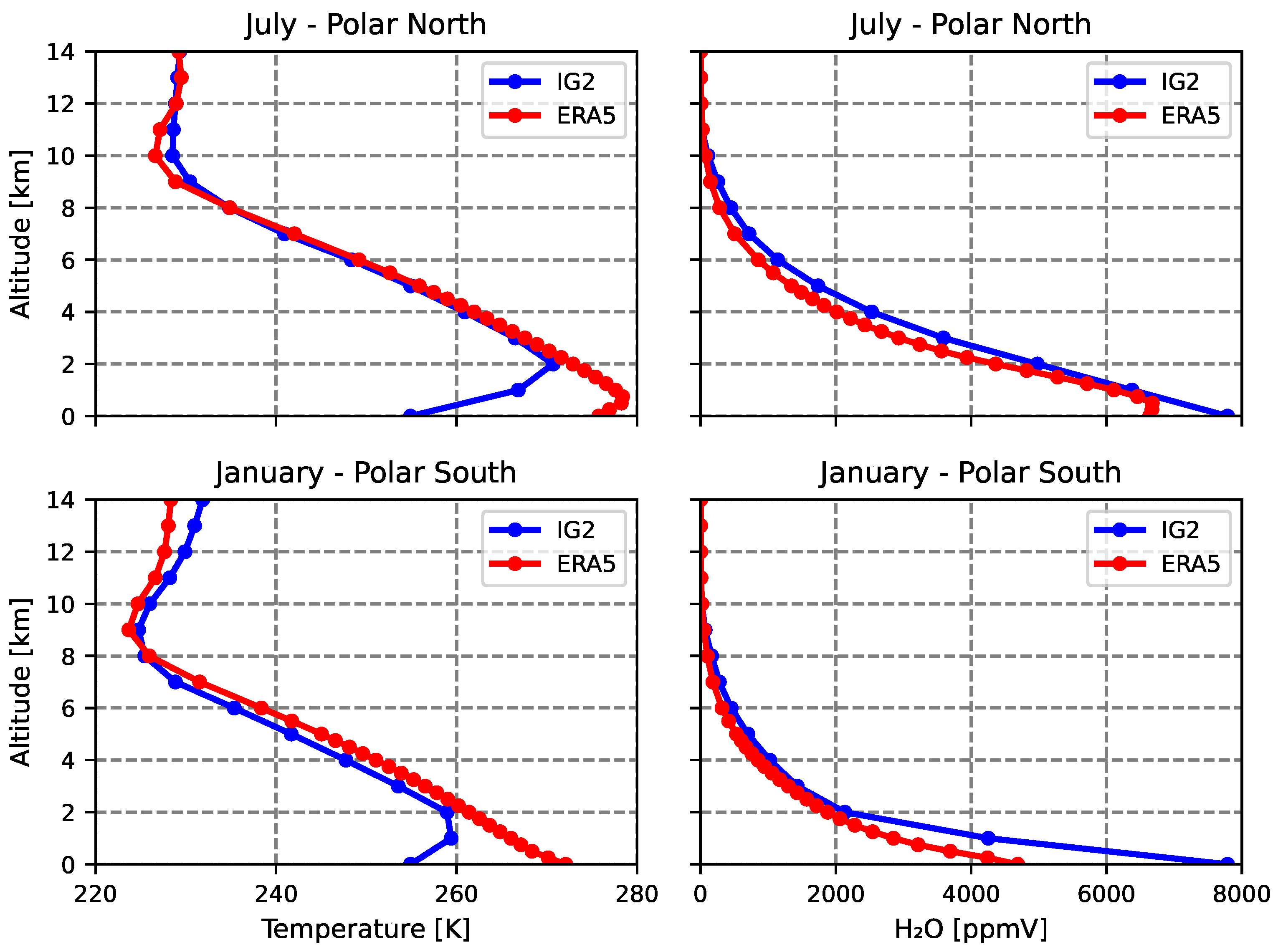
In general, there are significant differences between the ERA5 and the IG2 climatology, for both temperature and water vapour, especially in the lower part of the troposphere, mostly due to the fact that IG2 data incorporate both land and water surfaces, while the ERA5 data were selected above water surfaces only. As an example, in Figure 1, the ERA5 temperature (left panels) and water vapour (right panels) profiles for the summer season in the polar regions are compared to the original IG2 data in the altitude range from 0 to 14 km. Red lines represent the ERA5 data and blue lines the IG2 data. In the figure, the top panels refer to the Polar North region, and the bottom panels refer to the Polar South region. We see that there is a large difference at low altitudes for the temperature in both regions, while for water vapour, there is a large difference in the South and a smaller difference in the North.

6.3. Impact of the RTM Updates and Atmospheric Profiles on TCWV Retrieval

To assess the impact of the updates on the parameter calculation, we have used Sentinel 3A data, acquired during the first 10 days of July 2021. One year of data offers an exhaustive dataset to properly describe the latitudinal and seasonal variability in TCWV distribution. In addition, from internal tests, we observed that a specific month (i.e., July) can adequately represent the mean distribution of the same month in different years. Cloudy data were filtered out using the basic cloud mask. 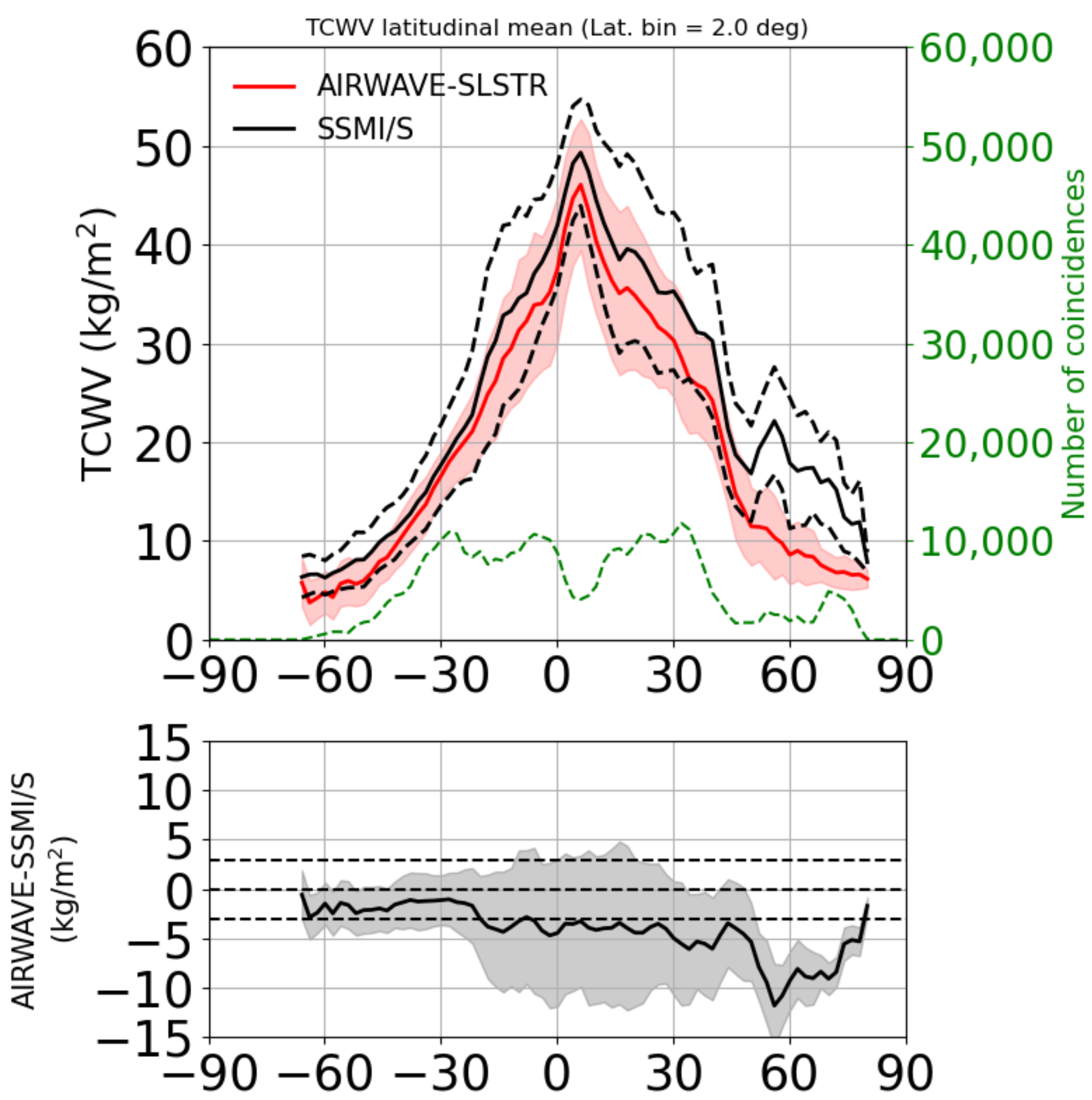The resulting TCWV were compared to the Special Sensor Microwave Imager/Sounder (SSMI/S) F17 coincident data [28], investigating the total bias, correlations, and latitudinal behaviour of the bias. In the comparison, only SSMI/S pixels where we had a 10% minimum coverage of the AIRWAVE data were used to avoid cloud contamination in SSMI/S data. To evaluate the effects of the updates, we use as reference data the TCWV obtained with the parameters computed with the original GBB code, HITRAN 2008 as spectroscopic data, and the MT_CKD version 2.5 as the water vapour continuum and the IG2 climatology. Figure 2 reports the results obtained in this configuration. In the upper panel, we report the latitudinal distribution of the average TCWV and its standard deviations for AIRWAVE-SLSTR (in red) and SSMI/S (in black). The green dashed line represents the number of coincidences used in the latitudinal average. The bottom panel shows the latitudinal distribution of the bias (AIRWAVE-SLSTR minus SSMI/S). With the reference parameters, the correlation between AIRWAVE and SSMI/S data was 0.92, and the average bias was about −3.93 kg/m${}^2$.

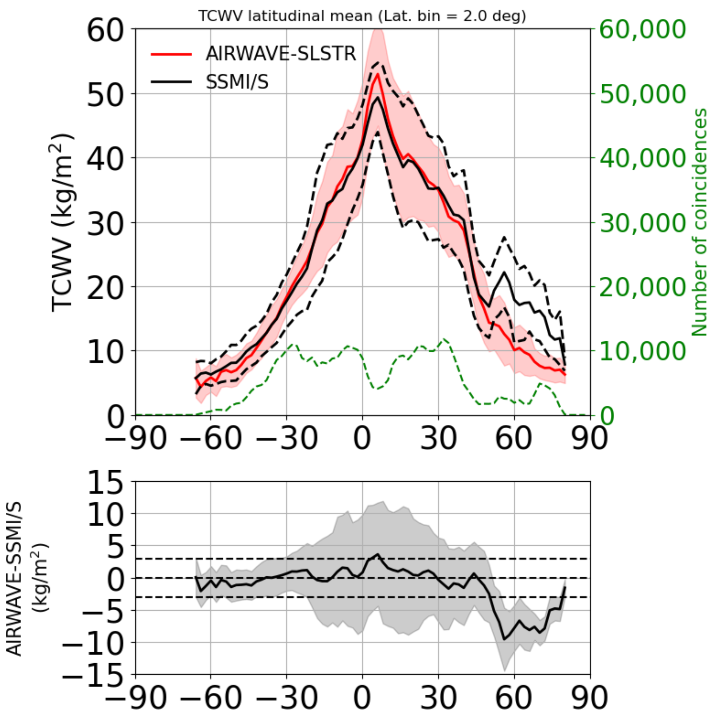
We then assessed the results obtained with the updates to the RTM (GBB-Nadir), the spectroscopic database, and the continuum model. Figure 3 shows similar plots to the ones in Figure 2, with the result obtained for this case. The bias with respect to SSMI/S decreased to −0.41 kg/m${}^2$ with a correlation of 0.92. The bias changed mainly in the tropical region, while almost no change was found at the poles. This behaviour is consistent with the fact that the effect of the new water vapour continuum is proportional to the water vapour atmospheric content that is larger at the equator.

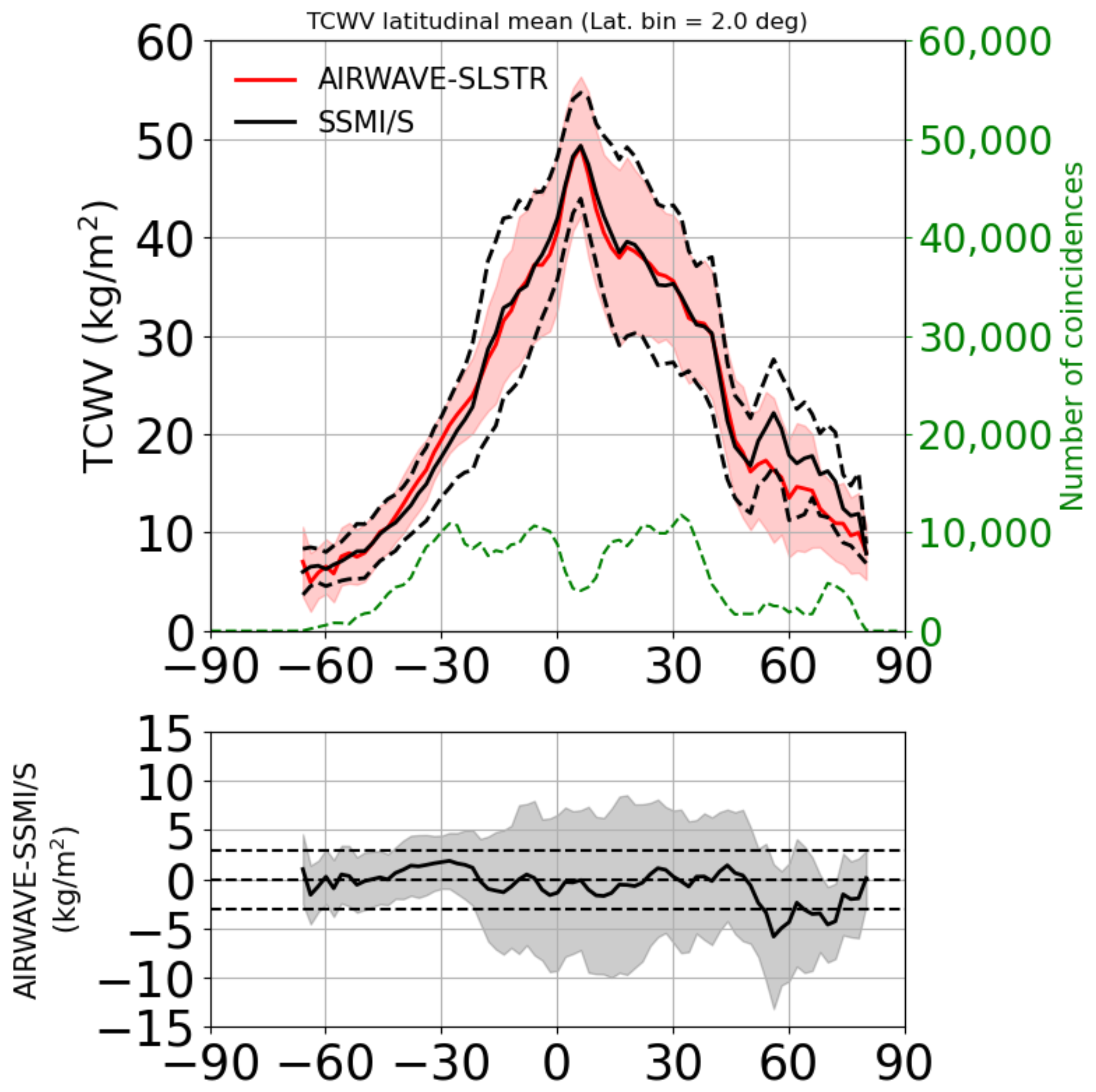
Finally, we calculated the parameters with the GBB-Nadir code and the ERA 5 profiles. The comparison is shown in Figure 4. With respect to the reference scenario, there was a definite improvement in the average bias, which became −0.12 kg/m${}^2$, with a correlation of 0.90. Moreover, the bias was almost constant at all latitudes, as can be clearly seen in the bottom panel of Figure 4.

6.4. Final Choices

All the tests performed on the July 2021 data showed that the updates to the RTM codes and to the atmospheric climatology resulted in an improvement in the AIRWAVE-SLSTR-retrieved TCWV. As a final check, we tested the new parameters on the SLSTR data measured in January, April, July, and October 2021, and we compared them to the results obtained with their previous version that was used in the AIRWAVE-for-SLSTR study.

Table 2. SLSTR performace vs. SSMI/S using the AIRWAVE-for-SLSTR (old, upper part of the table) retrieval parameters and the updated version (new, lower part of the table). Bias and STD are given in kg/m${}^2$.

AIRWAVE vs. SSMI	January 2021	April 2021	July 2021	October 2021
Old parameters
bias+/−STD	−3.12 ± 4.30	−3.09 ± 4.18	−3.75 ± 5.04	−2.92 ± 4.18
correlation	0.94	0.95	0.92	0.95
number of points	1,361,641	1,207,145	1,256,300	1,405,753
Updated parameters
Bias+/−STD	0.45 ± 4.70	−0.19 ± 4.49	−0.12 ± 5.64	−0.13 ± 4.13
correlation	0.93	0.95	0.90	0.95
number of points	1,351,717	1,200,433	1,252,402	1,403,065

reports the differences in the validation of the two versions of the TCWVs. In the table, we summarise the performances of the two sets of data using the bias and its STandard Deviation (STD), the Root Mean Square Estimate of the spread (RMSE), and the correlations with SSMI/S data.

On average, with the previous version of the AIRWAVE-for-SLSTR parameters, we had a bias of −3.22 kg/m${}^2$, a STD of 4.43 kg/m${}^2$, a RMSE of 5.47 kg/m${}^2$, and a high correlation (0.94). Using the new parameters, we obtain a much smaller bias (0.01 kg/m${}^2$—well within the accuracy requirements reported in Section 2), a STD of 4.74 kg/m${}^2$, a RMSE of 4.75 kg/m${}^2$, and 0.93 for the correlations. Thus, we obtain a significant improvement in the bias and an improvement in the RMSE. The correlation is similar, while with the updated configuration, we obtain a slightly larger STD. We have observed a residual latitudinal behaviour of the bias; however, considering the simplified assumption of six latitudes bands used in the AIRWAVE code, this is not critical.

The final choice of the climatology to be used in the calculation of the retrieval parameters is therefore the ERA5 cloud-free climatology, and the parameters have been computed with the updated code GBB-Nadir.

7. Results and Validation

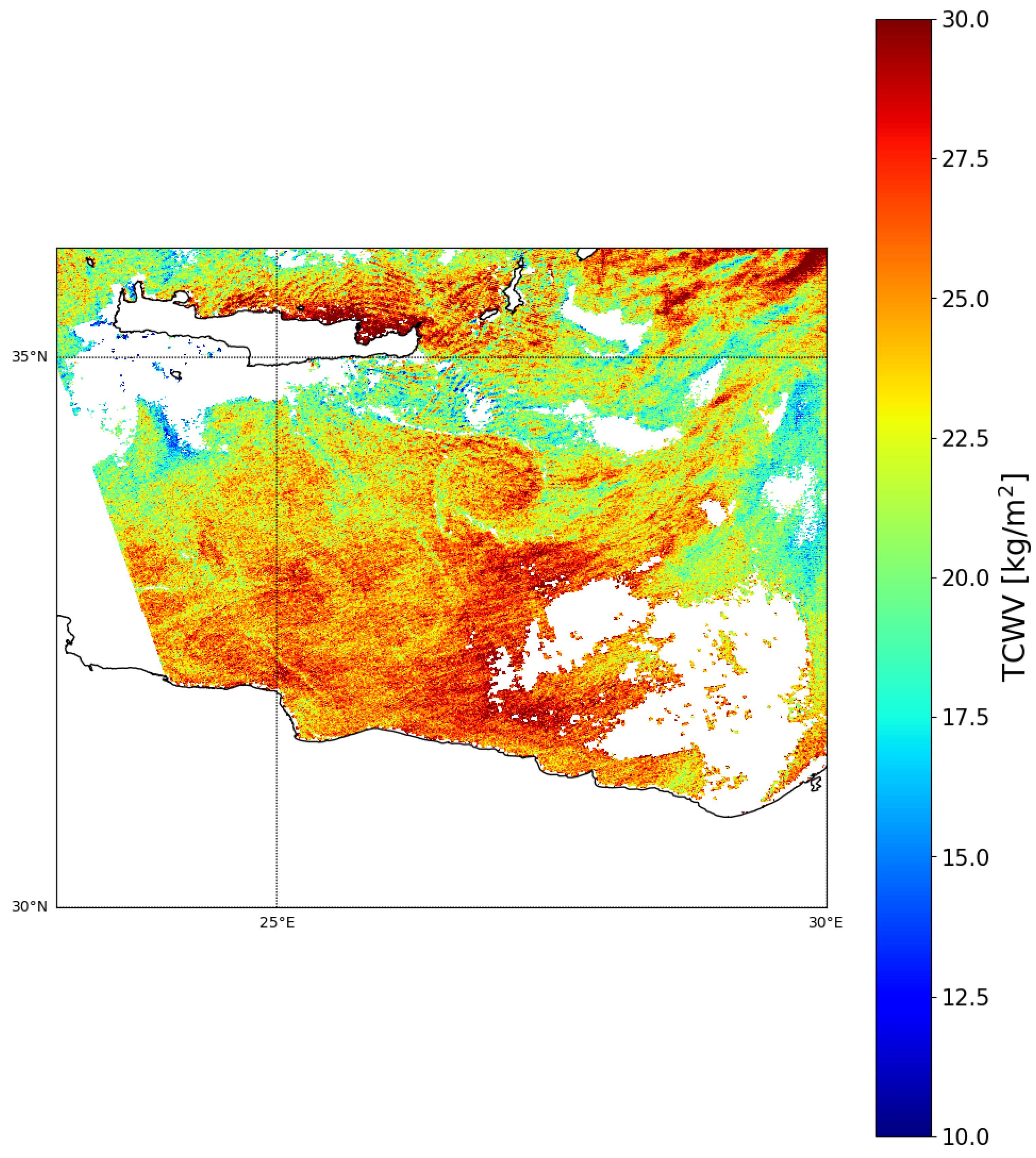
The final parameters were injected into the AIRWAVE-SLSTR algorithm and a full year (2021) of Sentinel 3-A (S3A) SLSTR measurements was processed. All the SLSTR measurements at their native resolution have been processed so that the different cloud masks available for the data could be applied post-processing. An example of the potentiality of the TCWV retrieved with AIRWAVE-SLSTR is shown in Figure 5, where we show the results of the retrieval of the S3A-SLSTR measurements over the East Mediterranean region on 5 July 2021, in its native resolution (1 × 1 km${}^2$). It was demonstrated by Papandrea et al. [29] that the TCWV retrieved with AIRWAVE from the AATSR measurements can be used to detect fine atmospheric structures like Lee Waves. 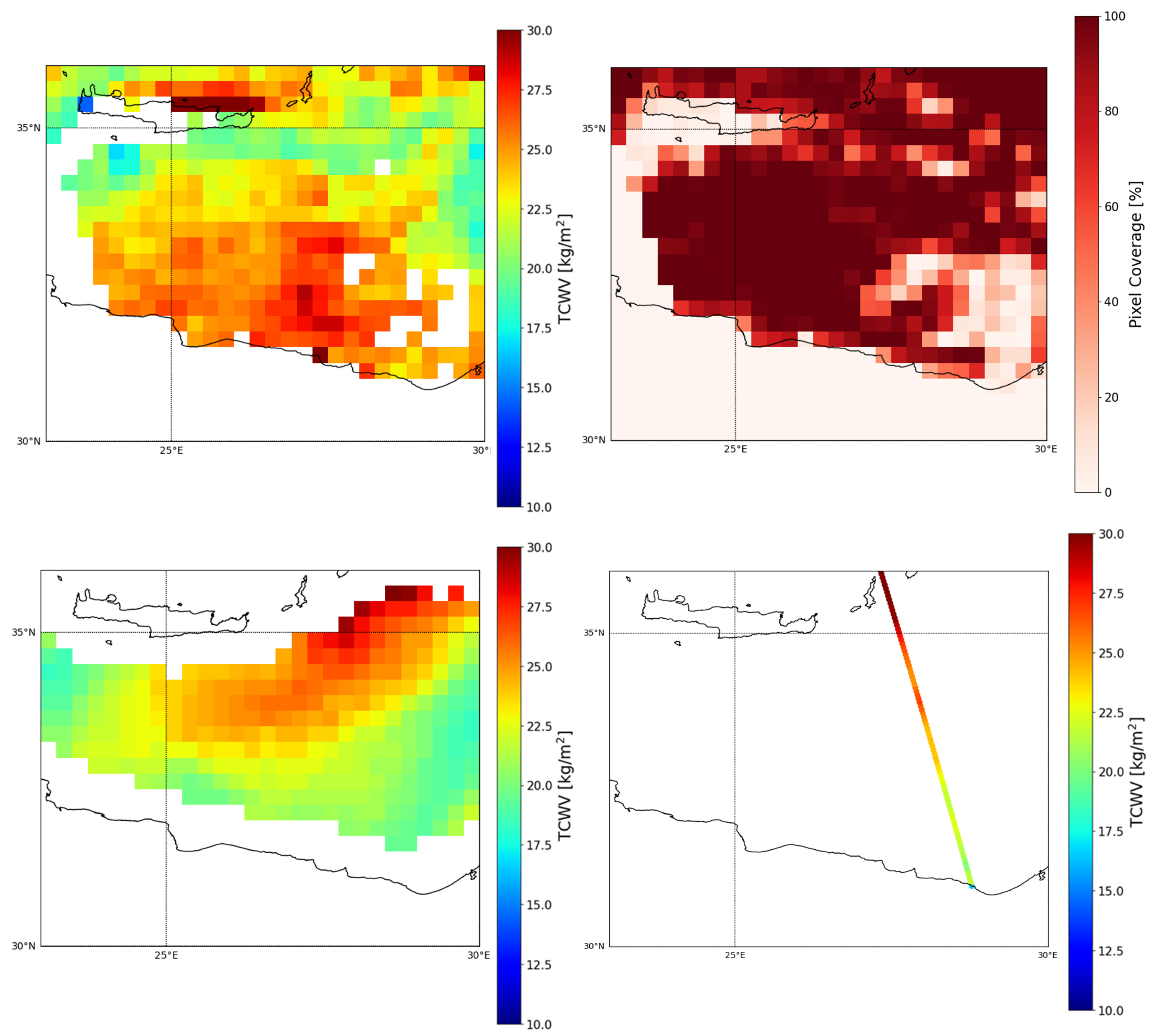The 1 × 1 km${}^2$ TCWV product shown in Figure 5 indeed shows Lee Waves near the Crete and Karpathos islands. If we compare these data with the top-left panel of Figure 6, where we have reported the same data re-gridded at the SSMI/S resolution, we see that the thin structures are no longer visible.

The AIRWAVE-SLSTR TCWV products for the full 2021 year have been validated by comparing them to similar TCWV products retrieved from the Remote Sensing System (RSS) SSMI/S [28], the MicroWave Radiometer (MWR) [12], the Integrated Global Radiosonde Archive (IGRA) coastal stations’ observations [30], and the AERONET (AErosol RObotic NETwork) observations [31]. The validation was performed using the SLSTR AIRWAVE Validation Dataset (SAVD), made using one year (2021) of Sentinel 3A AIRWAVE – SLSTR TCWV products. The SAVD contains more than 176,000 products, covering the entire globe, and it has been produced by processing SLSTR NTC L1b (baseline 004) data.

The SSMI/S products used in the validation are derived from the F17 satellite over water surfaces. We selected cloud-free SSMI/S data by excluding data with a Liquid Water Path (LWP) higher than zero, as a proxy of cloud presence. As already said in Section 6.3, the SSMI/S products are provided on a regular grid with a spatial resolution of 0.25${}^{°}$× 0.25${}^{°}$, so we averaged the high-resolution clear sky AIRWAVE-SLSTR TCWV data located in the area centred on each SSMI/S grid point. Since, at the time we processed the data, there were two cloud masks attached to the SLSTR L1b products, both the basic and the Bayesian, to select cloud-free measurements, we used both of them separately, and we evaluated the agreement between the two datasets when the clear sky Pixel Coverage (PC) for each SSMI/S grid cell was larger than 10%.

The IGRA dataset [30] used in the validation has been built considering only coastal stations where the sea coverage (percentage of sea surface area in a circle of 150 km radius around the location of each station) was larger than 20%. The stations located at an altitude higher than 250 m above the mean sea level were excluded from the analysis because they do not sample the lowest layers of the atmosphere. The AIRWAVE-SLSTR TCWV products were used at their native resolution of 1 × 1 km${}^2$. The maximum allowed distance between the IGRA station and the AIRWAVE-SLSTR products was 100 km, and the maximum time difference between the IGRA radio sounding and the Sentinel-3A overpass was set to 12 h. As for SSMI/S, only pixels with PC larger than 10% were used in the comparison.

The AERONET network (https://aeronet.gsfc.nasa.gov/, accessed on 13 March 2025) exploits the CIMEL CE318 sun–sky radiometer, a narrow band filter photometer capable of performing measurements of direct solar and diffuse sky irradiances at the selected wavelengths and at several scattering angles. The TCWV from this instrument is calculated using the official AERONET inversion algorithm [32]. From a review of the literature (see [33] and the references therein), the AERONET products were shown to have a mean negative bias of -5/-10%. As for the IGRA stations, the maximum allowed distance between the AERONET site and SLSTR measurements was 100 km. All the AERONET water vapour products within a time interval of ±30 min from the SLSTR sensing time have been considered. We have used only the AERONET sites surrounded by a percentage of sea surface higher than 20%. As for the validation against IGRA TCWV products, the stations located at an altitude higher than 250 m above the mean sea level were excluded.

The MWR instrument is on board the same satellite as SLSTR (Sentinel 3), and for the validation exercise, we could access only two months of co-located products, July and January 2021. It should be noted that during these two months, we have the most “problematic” agreement with all the reference datasets. The average FOV of the MWR instrument can be approximated by a circle with a radius of about 10 km; therefore, we selected all the native resolution clear sky AIRWAVE—SLSTR TCWV products within 10 km from the centre of the MWR IFOV. Since the distance between two contiguous MWR measurements is about the same as the radius of its swath, MWR swaths are partially superimposed. To reduce possible instabilities due to oversampling, we used only non-overlapping MWR data, therefore selecting one-third of the MWR available products. As in the SSMI/S validation, we excluded MWR products with a Liquid Water Path (LWP) higher than zero, as an MWR-derived proxy of cloud presence.

The results of the validation of the AIRWAVE-SLSTR TCWV products obtained with the new version of the parameters, with all the four datasets listed above, show an overall good agreement with correlation coefficients higher than 0.9. The bias is around 0 kg/m${}^2$ against SSMI/S, positive with respect to MWR and AERONET (about 1.5 kg/m${}^2$ and 0.7 kg/m${}^2$ respectively) and negative of about -1.7 kg/m${}^2$ against IGRA.

These validation parameters are summarised in

Table 3. Summary of the results of the validation of the AIRWAVE-SLSTR TCWV products against the different reference datasets. Both bias and STD are in kg/m${}^2$.

		SSMI/S	MWR *	IGRA	AERONET **
	Correlation	0.94	0.94	0.91	0.95
Basic	BIAS	0.00	1.33	−1.80	0.38
	STD	4.60	4.80	6.16	4.43
	Correlation	0.94	0.93	0.90	0.93
Bayesian	BIAS	0.43	1.73	−1.53	1.01
	STD	4.55	5.11	6.54	5.30

* The validation against MWR has been performed only in January and July 2021. ** The validation against AERONET has been performed using only day-time products.

for both the basic and the Bayesian cloud masks.

Moreover, to obtain insights into the improvement of new products, we compared the results of this validation against the results of previous validation exercises using SSMI/S and IGRA data. Formally, this comparison can be considered only qualitative because the considered periods are not the same. However, from all the tests we performed across the different AIRWAVE-SLSTR studies, we observed that the main outcomes (i.e., the mean bias and latitudinal distribution of the bias) from the analysis of one month are representative of the same month of other years. In the SSMI/S case, comparing two different one-year datasets that do not fully overlap, March 2020–April 2021, for the “old parameters” (v1) and January 2021–December 2021, for the “new parameters” (v2), we observed a significant improvement in terms of bias, with the overall bias obtained adopting the basic cloud mask changing from −3.32 kg/m${}^2$ (for v1) to 0 kg/m${}^2$ (for v2). Furthermore, in the IGRA case, despite the different periods considered (January, April, July, and October 2018 for v1; and January 2021–December 2021 for v2), a clear improvement is observed, with the bias changing from −4.8 to −1.8 kg/m${}^2$.

8. Discussion

Despite the reference datasets used in this validation exercise, by exploiting different retrieval methods and spectral ranges, we observed a good correlation between AIRWAVE-SLSTR and all the different reference datasets (larger than 0.90). The effects of the SLSTR cloud filtering (different cloud masks) on the agreement of the AIRWAVE-SLSTR TCWV products with the other datasets are similar. The mean biases are well within the ±3 kg/m${}^2$ interval. We found slightly larger biases (except when comparing the TCWV to the IGRA data) with the Bayesian cloud mask. In this case, the overall bias is 0.41 kg/m${}^2$, which, considering an average TCWV value of 30 kg/m${}^2$, corresponds to 1.4 %. At the same time, the standard deviation is 5.38 kg/m${}^2$, which corresponds to 17.9 %. Both results are within the ESA Water Vapour Climate Change Initiative requirements [9].

In the coastal areas, we generally observed a good agreement (±3 kg/m${}^2$), and in the cases where we observed major discrepancies, AIRWAVE-SLSTR tended to have a negative bias with respect to the reference products. This is evident in the validation against SSMI/S and IGRA, but also with the AERONET TCWV products, considering that, for AERONET, a bias of −5/−10% is reported in the literature. Despite a major improvement with respect to the results of the validation of the previous dataset, mainly in terms of the magnitude of the bias, a slight seasonality of the bias is still present, with the worst results observed in the summer hemisphere. The seasonality is more evident when SSMI/S and MWR are used for the validation of the AIRWAVE-SLSTR products. For ground-based references that do not properly cover the southern hemisphere, the major discrepancies are in the summer period of the northern hemisphere.

As an example of the comparison of AIRWAVE-SLSTR TCWV with the other satellite data, we use the same measurements shown in Figure 5. The top-left panel of Figure 6 reports the AIRWAVE-SLSTR data re-gridded at a SSMI/S resolution. The top-right panel of the same figure shows the number of AIRWAVE-SLSTR high resolution data averaged in each re-gridded pixel. Light pink areas correspond to cloudy pixels or to pixels near the border of the cloud. The representativeness of those pixels should be considered when comparing the AIRWAVE values to the ones obtained with MW sensors (SSMI/S and MWR). The SSMI/S TCWV values from the F17 satellite are reported in the bottom-left panel of Figure 6. SSMI/S shows smoother variations when compared to the AIRWAVE data; moreover, we can see that SSMI/S data are not available near the coasts (about 25 km) due to the land contamination effect in the SSMI/S FOV. Some differences in the retrieved values can be observed in regions where the PC is below 40%. Finally, the bottom-right panel of Figure 6 shows the MWR TCWV for the same SLSTR orbit. The 10 km FOV of MWR allows for retrieval in regions near the coasts that are not covered by the SSMI/S data. However, in this case, the Lee Waves and other thin atmospheric structures shown in AIRWAVE data are also not visible (e.g., the Lee Waves near the Karpathos island).

9. Conclusions

In this paper, we have described the algorithm AIRWAVE-SLSTR, the adaptation of the original AIRWAVE algorithm to the SLSTR measurements. The algorithm is designed to retrieve the TCWV from day- and night-time SLSTR measurements above water surfaces in clear sky conditions. The algorithm is an extension of the AIRWAVE algorithm, developed for the same purpose but for the ATSR instrument series. The steps performed to upgrade the original AIRWAVE algorithm have been thoroughly discussed. New retrieval parameters have been computed, exploiting the GBB-Nadir forward model, ’state-of-the-art’ spectroscopy, and the continuum models, and a new climatology, capable of deducing the average atmospheric and sea surface status during SLSTR measurements has been proposed. The algorithm has been applied to one year of SLSTR data (2021), and the obtained TCWV values have been validated using the coincident measurements of two satellites that operate within the microwave frequency region (SSMI/S and AMTROC-MWR). The correlation of the retrieved TCWV with the satellite measurements is 0.94, and the average bias is in the order of 0.66 kg/m${}^2$. The dataset has also been compared to ground-based measurements, using data from stations close to water surfaces. This validation has showed that the average correlation is 0.93 and the bias −0.48 kg/m${}^2$. The obtained accuracy is well within the requirements set for both numerical weather predictions (1–5 kg/m${}^2$) and for coastal altimetry applications (1.8–3 kg/m${}^2$). We have found the bias demonstrates a residual latitudinal dependence that is well within both the NWP and coastal altimetry requirements.

The work described in this paper confirms that the AIRWAVE-SLSTR algorithm can be successfully applied to SLSTR measurements (onboard any Sentinel-3 satellite in any illumination condition) to obtain a long time series of reliable TCWV values above the water surface, and it can extend the time series of TCWV derived from the ATSR instrument series.