Two-Stage Evapotranspiration Partitioning Under the Generalized Proportionality Hypothesis Based on the Interannual Relationship Between Precipitation and Runoff

Abstract

The generalized proportionality hypothesis (GPH) highlights the competitive relationships among hydrological components as precipitation (P) transforms into runoff (Q) and evapotranspiration (E), providing a novel perspective on E partitioning that differs from the traditional physical source-based approach. To achieve sequential partitioning of E into initial (E_i) and continuing (E_c) evapotranspiration under the GPH, a P-Q relationship-based E_i estimation method was proposed for the Model Parameter Estimation Experiment (MOPEX) catchments. On this basis, we analyzed the relationship between the GPH-based E components and the physical source-based ones separated by the Penman-Monteith-Mu algorithm. Additionally, we explored the differences between the calculated and inverse Budyko-WT model parameter (E_i/E) and discussed the implications for the Budyko framework. The results showed the following: (1) A significant linear P-Q relationship (p < 0.05) prevailed in the MOPEX catchments, providing a robust data foundation for E_i estimation. Across the MOPEX catchments, E_i and E_c contributed 73% and 27% of total E, respectively. (2) The combined proportion of evaporation from canopy interception and wet soil averaged about 25%, and it was much lower than that of E_i, indicating that it was difficult to establish a connection between E_i and the physical source-based E components. (3) The potential evapotranspiration (E_P) satisfying the Budyko-WT model was strictly constrained by the GPH, while the inappropriate E_P estimation method largely explained the discrepancy between the calculated and inverse E_i/E. This study deepens the knowledge of the sequential partitioning of E components, uncovers the discrepancies between different E partitioning frameworks, and provides new insights into the characterization of key variables in Budyko models.

1. Introduction

Land evaporation (E), also known as land evapotranspiration, is an important part of the hydrological cycle, and it plays a key role in regulating the exchange of water and energy between land and atmosphere [1,2,3]. A comprehensive understanding of E processes can help optimize water resource allocation and improve water use efficiency [4,5]. However, evapotranspiration is not a single process but comprises multiple processes, which can therefore be divided into several components [6,7]. Investigating the E components is essential for unveiling the complexity of E processes and enhancing the ability to predict the hydrological processes under the influence of climate change and human activities, which is particularly important for tackling the challenges posed by water scarcity and climate change.

Currently, E partitioning is often conceptualized based on its physical sources, with plant transpiration, soil evaporation, and canopy interception evaporation being considered as the main E components [8,9]. Some commonly used E models typically estimate the source-based E components first and then sum these components to obtain the total E values, such as the Priestley–Taylor jet propulsion laboratory (PT-JPL) [10] and variable infiltration capacity (VIC) [11] models. Many studies have explored the proportions of various physical source-based E components and their dynamic change over time [9,12,13,14,15].

Beyond partitioning by physical sources, the generalized proportionality hypothesis (GPH) offers an alternative perspective for dividing the E components. The GPH is derived from the precipitation (P) partitioning theory proposed by L’vovich [16], and it describes the dynamic competition between the water balance components. By applying the GPH to the division of P into E and runoff (Q) at the mean annual catchment scale, Wang and Tang [17] derived a parametric Budyko equation (i.e., the Budyko-WT equation) and demonstrated the applicability of the GPH across temporal scales from the Darwinian perspective. The GPH has recently seen a renaissance in the study of catchment hydrology [18,19,20,21,22,23].

According to the GPH, E can be partitioned into the initial (E_i) and continuing (E_c) evapotranspiration. E_i refers to the portion of E that originates from P before Q generation, while E_c represents the remaining part of E after Q generation. This partitioning captures the temporal dynamic characteristics of the hydrological cycle, emphasizing both the temporal sequence (i.e., whether E occurs before or after Q formation) and the competitive relationships (i.e., whether E competes with Q) inherent in the two-stage E processes. This is fundamentally different from the physical source-based E partitioning, which categorizes E components according to where and how evapotranspiration occurs, without considering the temporal characteristics of the process. In addition, it should be noted that the GPH-based E partitioning is generally applied at the mean annual catchment scale, while the physical source-based approach allows for much finer spatiotemporal scales, enabling analysis at daily and pixel levels. While previous studies have extensively explored the E partitioning from the perspective of its physical sources, investigations from the GPH perspective remain scarce. Furthermore, existing attempts to relate the GPH-based E components with the physical source-based ones have thus far relied on conceptual assumptions rather than empirical evidence [17,24]. The relationship between E components under these two partitioning frameworks is therefore worthy of quantitative exploration.

E_i is one of the E components under the GPH, and its ratio to E (E_i/E) not only represents the relative magnitude of its own contribution to total E but also serves as the Budyko-WT model parameter [17]. Unlike other Budyko models, such as the Budyko–Fu [25,26] and the Budyko-MCY [27,28,29], whose parameters are introduced as mathematical integration variables without explicit physical interpretation, the GPH-based Budyko-WT model features a parameter (E_i/E) with a clear physical meaning, as both E_i and E are physically defined quantities with fixed values that can be determined for a specific catchment and time period. This physical basis provides the potential for directly estimating E_i/E through physical processes. For the applications of the Budyko-WT model oriented toward E estimation, given known values of P and potential evapotranspiration (E_P), E can be obtained once E_i is determined, which, in effect, determines the model parameter. Thus, exploring an approach for E_i estimation not only aids in clarifying the partitioning characteristics of GPH-based E components but also facilitates the determination of the Budyko model parameter, which is crucial for advancing both the understanding and the applications of the Budyko framework.

The primary objective of this study was to explore the temporal dynamic characteristics of E processes under the GPH. Towards this, we took the Model Parameter Estimation Experiment (MOPEX) catchments as the study area and proposed an E_i estimation method based on the P-Q relationship by considering its physical meaning. After E_i was determined using this method, E_c was obtained subsequently, thus enabling the GPH-based E partitioning. On this basis, we separated the physical source-based E components by the Penman-Monteith-Mu (PM-Mu) algorithm [30,31,32] to analyze the relationship between E components under two E partitioning frameworks. Finally, we examined the relationship between the inverse and calculated values of the parameter E_i/E of the GPH-based Budyko-WT model.

2. Materials and Methods

2.1. Hydrometeorological and Remote Sensing Data

The MOPEX dataset contains daily P and Q data during 1948–2003 of 438 catchments across the contiguous United States [33] and has been widely used in catchment-scale hydrological studies [34,35,36,37]. Considering the time span of the auxiliary climate and vegetation datasets used in this study, we restricted all data to the overlapping period of 1982–2003. Daily-scale P and Q were aggregated to the annual scale, and 66 catchments with less than 11 years of data were excluded. Upon inspection, the data for the remaining 372 catchments all met the water balance constraint at the mean annual scale (i.e., P > Q). The temporal scale of 11 years was chosen because previous studies [38,39,40] demonstrated that the terrestrial water storage variation can be approximately ignored at scales longer than 11 years, allowing E to be derived from the water balance equation (i.e., E = P − Q). Then, we examined the linear P-Q relationship for each catchment. Catchments were deleted with a slope outside the interval (0, 1), an insignificant relationship (p > 0.05), or a negative P-axis intercept. In total, 29 catchments were removed, leaving 343 catchments for further analysis (Figure 1). This removal was based on physical and methodological considerations to ensure the applicability of the E_i estimation. The remaining 343 catchments span a wide range of natural geographical and hydro-meteorological conditions, providing a representative basis for analysis. The data length for these catchments ranged from 11 to 22 years, with a median of 20 years.

We also acquired the gridMET meteorological dataset [41], the Global Land Surface Satellite (GLASS) fraction of vegetation coverage (F_C) [42] and land surface albedo [43] data, and the Global Inventory Modeling and Mapping Studies (GIMMS) leaf area index (LAI) data [44,45] to serve as input for the PM-Mu algorithm (Section 2.4). These datasets are detailed in

Table 1. Information of the datasets used in this study.

Dataset	Spatial Resolution	Temporal Resolution	Time Span	Reference	Data Access Weblink
MOPEX catchment hydrological data	Catchment scale	Daily	1948–2003	[33]	ftp://hydrology.nws.noaa.gov/pub/gcip/mopex/US_Data/ (accessed on 21 October 2022)
High-resolution meteorological data gridMET	4 km	Daily	1979–2021	[41]	https://www.climatologylab.org/gridmet.html (accessed on 25 February 2023)
GLASS FC	0.05°	8 days	1982–2020	[42]	http://www.glass.umd.edu/Download.html (accessed on 2 June 2023)
GLASS albedo	0.05°	8 days	1982–2020	[43]	http://www.glass.umd.edu/Download.html (accessed on 2 June 2023)
GIMMS LAI	1/12°	Half month	1982–2020	[44,45]	https://zenodo.org/records/8281930 (accessed on 2 June 2023)

Note: F_C = fraction of vegetation coverage. LAI = leaf area index.

. In addition, the gridMET meteorological data were also used to calculate E_P (Section 2.5).

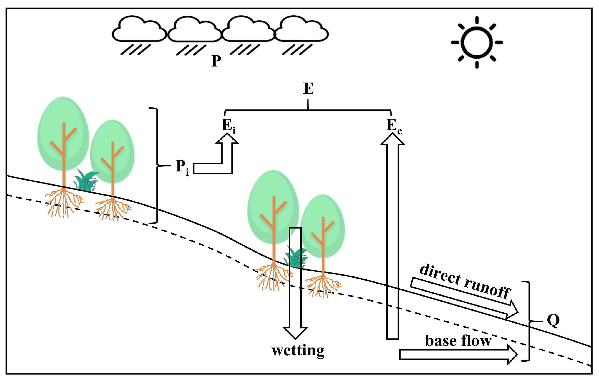
2.2. Generalized Proportionality Hypothesis and Budyko-WT Equation

As shown in Figure 2, precipitation at the event scale falls to the ground and then first satisfies the demand of initial abstraction (P_i), such as canopy interception and water storage in top soils. The remaining water represents surface runoff and continuing abstractions. The proportionality hypothesis of the Soil Conservation Service (SCS) curve number method is that the ratio of surface runoff to its potential is equal to that of continuing abstraction to its potential [46]. Ponce and Shetty [47] extended this hypothesis to hydrological processes similar to event-scale precipitation partitioning and obtained the GPH. Wang and Tang [17] creatively applied the GPH to hydrological partitioning at the mean annual catchment scale and demonstrated its universality across temporal scales.

At the mean annual scale, P has a priority to meet the demand for E_i, which includes but is not limited to the evapotranspiration from leaf interception and the wet topsoil layer. The remaining available water not taken up by E_i goes to continuing infiltration and surface runoff (or direct runoff). Part of the continuing infiltration is eventually evaporated, called the continuing evapotranspiration (E_c), and the other part forms the base flow. E_i and E_c constitute E, while the surface runoff and base flow constitute Q. No runoff is produced during the first stage. According to the GPH that the ratio of E_c to its potential is equal to that of Q to its potential, a mathematical expression is obtained to describe the competitive relationship among the water balance components [17,48]:

$${\displaystyle \frac{\mathrm{E}-{\mathrm{E}}_{\mathrm{i}}}{{\mathrm{E}}_{\mathrm{P}}-{\mathrm{E}}_{\mathrm{i}}}}={\displaystyle \frac{\mathrm{Q}}{\mathrm{P}-{\mathrm{E}}_{\mathrm{i}}}}$$

(1)

The Budyko-WT equation [17] can be further derived:

$${\displaystyle \frac{\mathrm{E}}{\mathrm{P}}}={\displaystyle \frac{1+{\mathrm{E}}_{\mathrm{P}}/\mathrm{P}-\sqrt{{(1+{\mathrm{E}}_{\mathrm{P}}/\mathrm{P})}^2-4\mathrm{m}(2-\mathrm{m}){\mathrm{E}}_{\mathrm{P}}/\mathrm{P}}}{2\mathrm{m}(2-\mathrm{m})}}$$

(2)

where m = E_i/E, with a range of [0, 1]. It modifies the partitioning of E into E_i and E_c and that of P into E and Q.

According to Equation (1) or Equation (2), the inverse E_i (E_i-inv) can be obtained:

$${\mathrm{E}}_{\mathrm{i}-\mathrm{i}\mathrm{n}\mathrm{v}}=\mathrm{E}-\sqrt{(\mathrm{P}-\mathrm{E})({\mathrm{E}}_{\mathrm{P}}-\mathrm{E})}$$

(3)

Dividing both sides of the above equation by E yields the inverse m (m_inv):

$${\mathrm{m}}_{\mathrm{i}\mathrm{n}\mathrm{v}}=1-\sqrt{(1-\mathrm{P}/\mathrm{E})(1-{\mathrm{E}}_{\mathrm{P}}/\mathrm{E})}$$

(4)

The key to the E partitioning under the GPH is the estimation of E_i. To achieve the partitioning, we first propose an E_i estimation method based on the P-Q relationship (Section 2.3). After E_i is determined using this approach, E_c is computed as the difference between E and E_i.

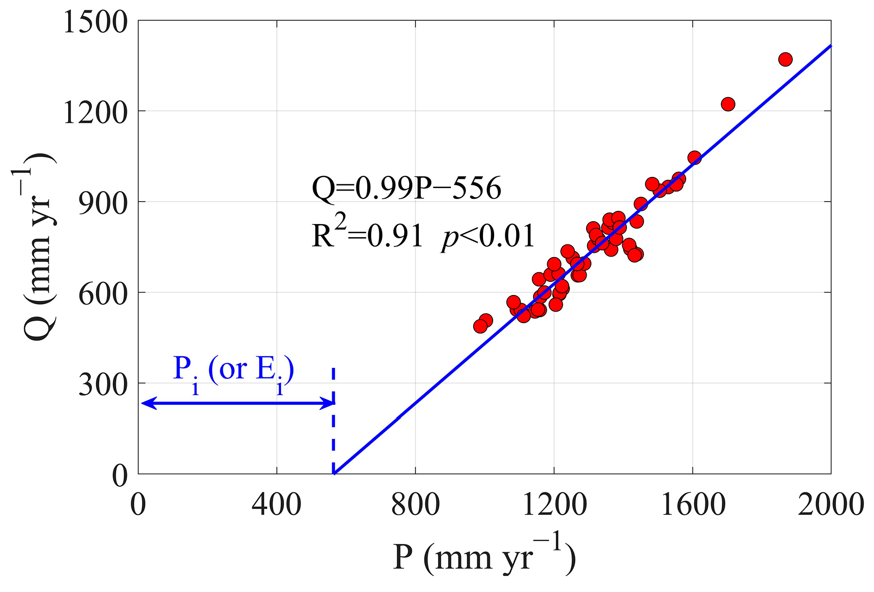
2.3. E_i Estimation Based on Catchment P-Q Relationship

According to Wang and Tang [17], runoff is typically not generated immediately upon precipitation but begins only after a certain threshold is reached. This critical value is called the initial abstraction in the event-scale SCS curve number method and is equal to E_i at the mean annual scale. That is, precipitation first meets the demand of E_i, and the remaining water is reserved for the competition between runoff and E_c [17]. In other words, E_i is the portion of evapotranspiration from precipitation that does not participate in runoff formation.

Previous studies have shown that Q generally increases with P at the catchment scale, so there are usually significant positive relationships between annual P and Q. Most of these relationships can be expressed as linear functions [49,50,51,52,53], while a few are expressed as nonlinear functions [54,55,56].

For a given catchment with a linear P-Q relationship, the linear regression equation is as follows:

$$\mathrm{Q}=\mathrm{k}\mathrm{P}+\mathrm{b}$$

(5)

It can be rewritten as follows:

$$\mathrm{Q}=\mathrm{k}(\mathrm{P}+\mathrm{b}/\mathrm{k})$$

(6)

where k is the slope of the linear P-Q relationship with the range of (0,1).

Generally, runoff occurs when P exceeds a certain value, implying a negative b. Let P_i = −b/k be the critical amount of P before runoff starts, and it is equal to the initial abstraction in the SCS curve number method. When P decreases to P_i, the annual runoff is zero. This reflects an extreme case of interannual variation of P and Q. On the other hand, since the mean annual P and Q (i.e., $\overline{\mathrm{P}}$ and $\overline{\mathrm{Q}}$) are also on the regression line (Equation (6)) (i.e., $\overline{\mathrm{Q}}=\mathrm{k}(\overline{\mathrm{P}}-{\mathrm{P}}_{\mathrm{i}})$), P_i is also the initial abstraction at the mean annual scale from the perspective of segmenting annual P and is therefore equal to E_i.

Figure 3 illustrates the E_i estimation based on the linear P-Q relationship for a randomly selected catchment. For this catchment, Q begins when P gradually increases from zero to a critical value P_i (549.09 mm yr⁻¹). Then, Q increases with P. This threshold represents the portion of precipitation that is first allocated to evapotranspiration before any runoff occurs, namely E_i.

2.4. Estimation of E Components Based on Penman-Monteith-Mu Algorithm

Here, we used the PM-Mu algorithm to estimate the physical source-based E components [30,31,32]. The algorithm is driven by climate and remote sensing vegetation data, with E being the sum of canopy interception evaporation (E_wc), vegetation transpiration (E_t), and soil evaporation (E_s), where E_s includes (saturated) wet soil evaporation (E_ws) and (unsaturated) moist soil evaporation (E_ms). This finer partitioning enables a more detailed examination of the relationship between E_i and the physical source-based E components. In addition, the PM-Mu algorithm has been shown to perform well in estimating E globally [57]. The corresponding equations are as follows:

$$\mathrm{E}={\mathrm{E}}_{\mathrm{w}\mathrm{c}}+{\mathrm{E}}_{\mathrm{t}}+{\mathrm{E}}_{\mathrm{s}}$$

(7)

$${\mathrm{E}}_{\mathrm{w}\mathrm{c}}={\displaystyle \frac{(∆·{\mathrm{R}}_{\mathrm{n}}+\mathsf{\rho }{·\mathrm{C}}_{\mathrm{p}}·\mathrm{V}\mathrm{P}\mathrm{D}/{\mathrm{r}}_{\mathrm{h}\mathrm{r}\mathrm{c}})·{\mathrm{F}}_{\mathrm{C}}·{\mathrm{F}}_{\mathrm{w}\mathrm{e}\mathrm{t}}}{∆+\mathsf{\gamma }\frac{{\mathrm{r}}_{\mathrm{v}\mathrm{c}}}{{\mathrm{r}}_{\mathrm{h}\mathrm{r}\mathrm{c}}}}}/\mathsf{\lambda }$$

(8)

$${\mathrm{E}}_{\mathrm{t}}={\displaystyle \frac{(∆·{\mathrm{R}}_{\mathrm{n}}+\mathsf{\rho }{·\mathrm{C}}_{\mathrm{p}}·\mathrm{V}\mathrm{P}\mathrm{D}/{\mathrm{r}}_{\mathrm{a}})·{\mathrm{F}}_{\mathrm{C}}·{(1-\mathrm{F}}_{\mathrm{w}\mathrm{e}\mathrm{t}})}{∆+\mathsf{\gamma }(1+\frac{{\mathrm{r}}_{\mathrm{s}}}{{\mathrm{r}}_{\mathrm{a}}})}}/\mathsf{\lambda }$$

(9)

$${\mathrm{E}}_{\mathrm{s}}={\mathrm{E}}_{\mathrm{w}\mathrm{s}}+{\mathrm{E}}_{\mathrm{m}\mathrm{s}}$$

(10)

$${\mathrm{E}}_{\mathrm{w}\mathrm{s}}={\displaystyle \frac{(∆·{\mathrm{R}}_{\mathrm{n}}+\mathsf{\rho }{·\mathrm{C}}_{\mathrm{p}}·\mathrm{V}\mathrm{P}\mathrm{D}/{\mathrm{r}}_{\mathrm{a}\mathrm{s}})·(1-{\mathrm{F}}_{\mathrm{C}})·{\mathrm{F}}_{\mathrm{w}\mathrm{e}\mathrm{t}}}{∆+\mathsf{\gamma }\frac{{\mathrm{r}}_{\mathrm{t}\mathrm{o}\mathrm{t}}}{{\mathrm{r}}_{\mathrm{a}\mathrm{s}}}}}/\mathsf{\lambda }$$

(11)

$${\mathrm{E}}_{\mathrm{m}\mathrm{s}}={\displaystyle \frac{(∆·{\mathrm{R}}_{\mathrm{n}}+\mathsf{\rho }{·\mathrm{C}}_{\mathrm{p}}·\mathrm{V}\mathrm{P}\mathrm{D}/{\mathrm{r}}_{\mathrm{a}\mathrm{s}})·(1-{\mathrm{F}}_{\mathrm{C}})·(1-{\mathrm{F}}_{\mathrm{w}\mathrm{e}\mathrm{t}})}{∆+\mathsf{\gamma }\frac{{\mathrm{r}}_{\mathrm{t}\mathrm{o}\mathrm{t}}}{{\mathrm{r}}_{\mathrm{a}\mathrm{s}}}}}{\left(\mathrm{R}\mathrm{H}\right)}^{{\displaystyle \frac{\mathrm{V}\mathrm{P}\mathrm{D}}{\mathsf{\beta }}}}/\mathsf{\lambda }$$

(12)

where $∆$ is the slope of the saturation vapor pressure curve at the air temperature (kPa °C⁻¹). R_n is the net radiation (MJ m⁻² day⁻¹). F_wet is the water cover fraction, calculated using the relative humidity. $\mathsf{\lambda }$ is the latent heat of vaporization (kPa °C⁻¹), which is a function of air temperature. VPD denotes the vapor pressure deficit (kPa). $\mathsf{\rho }$ is the air density, with a value of 1.29 kg m⁻³. C_P is the specific heat capacity of air, with a value of 1.013 × 10⁻³ MJ kg⁻¹ °C⁻¹. $\mathsf{\gamma }$ is the psychometric constant (kPa °C⁻¹). $\mathsf{\beta }$ is an empirical coefficient, with a value of 250. r_vc and r_hrc are wet canopy resistance and aerodynamic resistance to evaporated water on the wet canopy surface (s m⁻¹). r_s and r_a are surface resistance and aerodynamic resistance (s m⁻¹). r_tot and r_as are total aerodynamic resistance to vapor transport and aerodynamic resistance at the soil surface (s m⁻¹). For detailed calculations, please refer to relative references [31,58,59].

Based on the PM-Mu algorithm, we estimated four components of E at the pixel and daily scales across the contiguous United States during 1982–2003, and the annual values of each component and total E were obtained by summing the daily values. Due to the lack of observational data for validating of each component, we used the catchment water balance-based E (E_wb) to validate the E estimated by the PM-Mu algorithm (E_pm), which was a widely adopted approach for validating E estimates [60,61]. We then analyzed the relationship between E_i and the physical source-based E components. It should be noted that the PM-Mu algorithm mainly focuses on the vegetation ecosystem, and it does not estimate E for the non-vegetation pixels, such as water bodies, perennial snow/ice, sparse vegetation (rock, tundra, and desert), and urban/built-up areas [59,62]. Therefore, we further excluded the catchments containing non-vegetation pixels when evaluating the E estimation performance and analyzing E components. To ensure comparability, the temporal coverage of data for the resulting 211 MOPEX catchments involved in E validation and component analysis were completely consistent.

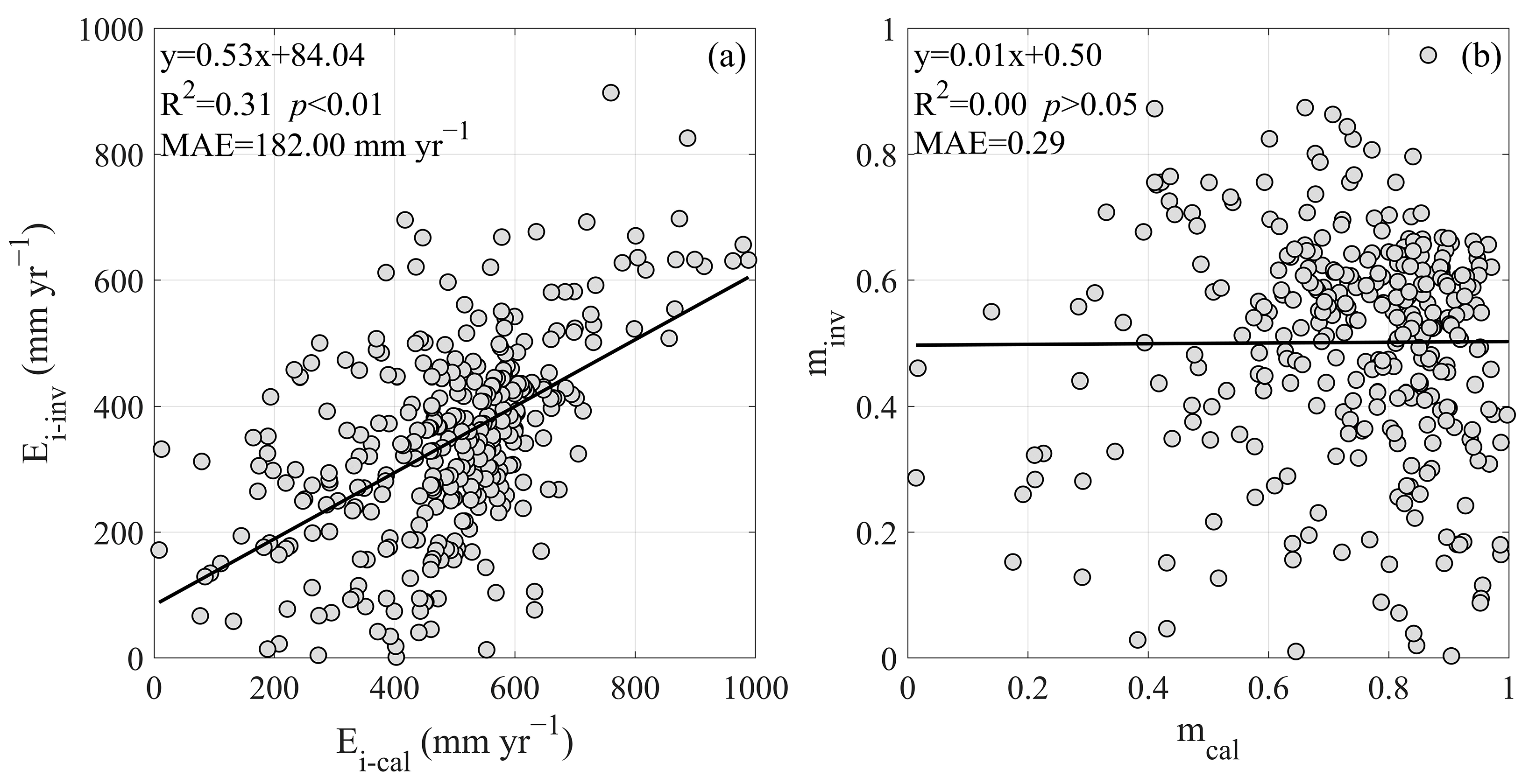
2.5. Comparison of the Inverse and Calculated Budyko-WT Model Parameter

The ratio of E_i to E not only represents the proportion of E components under the GPH but also serves as the Budyko-WT model parameter (m). In Budyko-related studies, the model parameter is typically derived from known P, E, and E_P. Inverse values of the model parameter are commonly used to establish empirical formulas [63,64] or to extrapolate to ungauged periods or catchments directly [65,66] for E simulation. Estimating E_i based on the linear P-Q relationship offers an alternative method for determining the Budyko model parameter, with the resulting E_i and m denoted as E_i-cal and m_cal, respectively, both representing the calculated values.

Here, we calculated E_P using the Priestley-Taylor equation [67] and then obtained the inverse E_i (i.e., E_i-inv) by Equation (3) and the inverse Budyko-WT model parameter (i.e., m_inv) by Equation (4). We subsequently compared the relationship between E_i-inv and m_inv with the calculated ones. E_P was calculated as follows:

$${\mathrm{E}}_{\mathrm{P}}=\mathsf{\alpha }{\displaystyle \frac{\mathsf{\Delta }}{\mathsf{\Delta }+\mathsf{\gamma }}}({\mathrm{R}}_{\mathrm{n}}-\mathrm{G})/\mathsf{\lambda }$$

(13)

where α is the Priestley-Taylor coefficient, typically set to 1.26 [67]. G is the soil heat flux (MJ m⁻² day⁻¹), which is often neglected at the daily scale.

3. Results

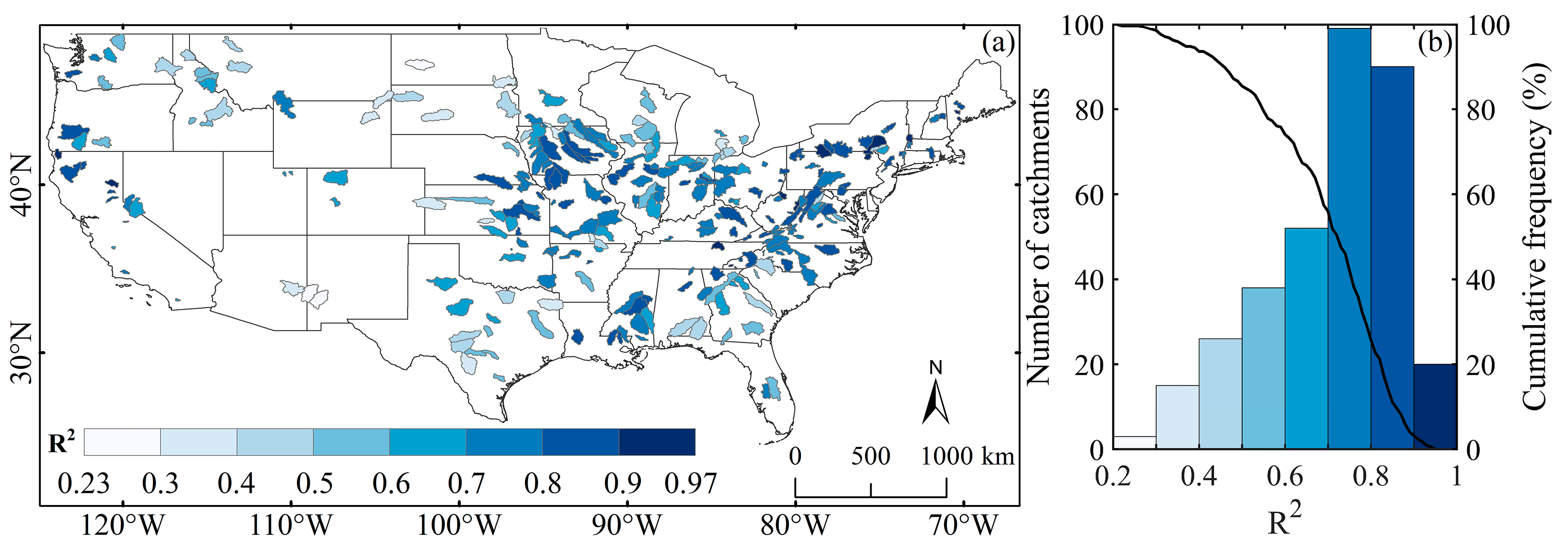
3.1. Linear Characteristics of the P-Q Relationship in MOPEX Catchments

The spatial distribution and frequency statistics of the coefficient of determination (R²) of the linear P-Q relationship for the MOPEX catchments are shown in Figure 4. It can be observed that a generally linear P-Q relationship prevailed throughout the MOPEX catchments. After excluding the catchments with missing data, about 92% (343 out of 372) of the MOPEX catchments showed a significant linear P-Q relationship (p < 0.05). Among the 343 catchments remaining after the screening, the R² of the linear P-Q relationship was greater than 0.50 for about 87% of the catchments, and for more than 50% of the catchments, the R² exceeded 0.74. This indicates that the linear function effectively captured the annual P-Q relationship in the MOPEX catchments, providing a solid data foundation for estimating catchment E_i based on the linear P-Q relationship.

3.2. Spatial Patterns of E_i and E_c in MOPEX Catchments

After E_i was determined based on the linear P-Q relationship, E_c was obtained by the difference between E and E_i. Figure 5 shows the spatial distribution of E_i, E_c, and the proportion of E_i to E. Overall, E_i was larger than E_c, and their mean values across 343 MOPEX catchments were 478.45 ± 173.73 (mean ± standard deviation) and 170.38 ± 118.78 mm yr⁻¹, respectively. In terms of proportions, the average E_i/E was 73% ± 20%, while the average E_c/E, as its complement, was 27% ± 20%. Spatially, higher E_i values were concentrated in catchments in eastern and southeastern areas of the contiguous United States (Figure 5a), and these catchments generally exhibited higher E_i proportions, with many exceeding 80% (Figure 5c). The overall spatial pattern of E_c (Figure 5b) was opposite to that of E_i.

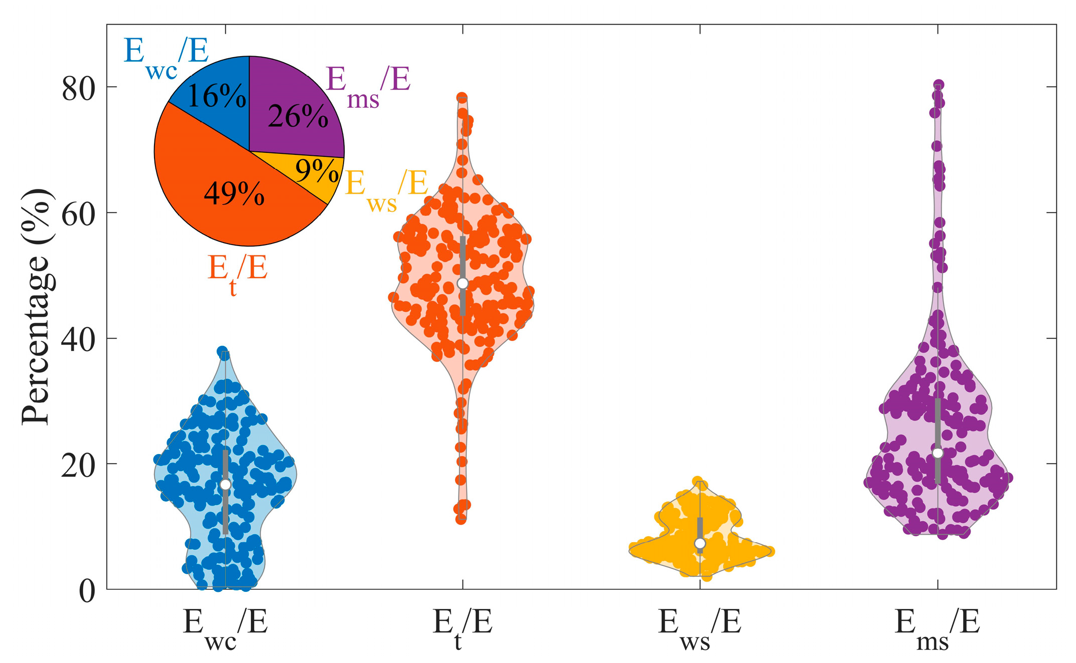
3.3. Relationship of E Components Between Two Partitioning Frameworks

The PM-Mu algorithm was employed to estimate the physical source-based E components, which were then summed to yield the total E. We first evaluated the performance of the PM-Mu algorithm in E estimation. As indicated by the comparison in Figure 6, there was a significant linear relationship between E_pm and E_wb (R² = 0.59, p < 0.01), with the mean absolute error (MAE) of 192.56 mm yr⁻¹. The estimation performance was comparable to that reported by Mu, Zhao, and Running [31] for the PM-Mu algorithm in the contiguous United States. By and large, the good agreement between E_pm and E_wb suggests that the PM-Mu algorithm performed adequately in estimating E for the MOPEX catchments.

The proportions of each component of E are shown in Figure 7. For 221 MOPEX catchments participating in E validation and component analysis, the average proportions of E_wc, E_t, E_ws, and E_ms derived from the PM-Mu algorithm were about 16% ± 9%, 49% ± 11%, 9% ± 3% and 26% ± 14%, respectively. In some studies, E_i was calculated as the sum of E_wc and E_ws [24,57]. For 221 MOPEX catchments, the average (E_wc + E_ws)/E obtained based on the PM-Mu algorithm was about 25%, markedly lower than the average E_i/E (74%) obtained using the linear P-Q relationship in this study. Specifically, in 216 of the 221 catchments, the total proportion of E_wc and E_ws was less than the proportion of E_i.

E_i is defined as the portion of evapotranspiration from precipitation that does not participate in the runoff formation and is characterized as not competing with the portion of precipitation used to produce runoff. Wang and Tang [17] suggested that E_i includes but is not limited to evaporation that occurs due to vegetation interception and water storage in top soils. This itself indicates that E_wc and E_ws are insufficient to constitute the entirety of E_i. In addition, we noticed that under the limiting case, the Buyko-WT model parameter E_i/E can take the value of unity. In this case, E = E_i, implying that E_i encompasses all the physical source-based E components. Therefore, upon comprehensive consideration, the assumption that E_i = E_wc + E_ws is not appropriate, and it is difficult to establish a direct correspondence between E_i and the physical source-based E components.

3.4. Comparison Between the Inverse and Calculated E_i/E

E_i and E_i/E were derived from P, Q, and E_P (Equation (13)) by Equation (1) or (2). There were 20 catchments with negative E_i-inv and corresponding negative m_inv. In the Budyko space, the data points (E_P/P, E/P) for these catchments fell below the lower bound of the Budyko-WT curves (i.e., m = 0). Clearly, this lacked physical significance. From Equation (4), we found that when E_P > P(P − Q)/Q, E_i-inv would be negative. This indicates that the E_P satisfying the Budyko-WT model should be smaller than P(P − Q)/Q. However, as we all know, E_P estimation from different meteorological equations varies in magnitude [68,69]. As can be expected, when a larger E_P is used, E_i-inv is more likely to be negative, thereby limiting the applications of the Budyko-WT model.

After excluding the catchments with negative E_i-inv, we compared the inverse and calculated values of E_i and m, respectively. As shown in Figure 8, although there existed a significant linear relationship between E_i-inv and E_i-cal (p < 0.01), the R² was relatively low (0.31), and the regression line also deviated substantially from the 1:1 line. The data points of m_inv and m_cal were scattered, and their relationship was not statistically significant (p > 0.05). The discrepancy in m is mainly attributed to the improper estimation of E_P. In Budyko-related studies, the model parameter is typically inverted by known P, E, and E_P [65,70]. For a given catchment during a given period, P and Q are fixed, so E is determined by the water balance equation. However, in practical applications, various methods are available for E_P estimation, leading to discrepancies in its values and, consequently, differences in the Budyko model parameter values. In other words, inverting the model parameter inherently implies that it varies with the chosen E_P. This approach is feasible for the Budyko-Fu and Budyko-MCY models, where their model parameters do not possess a clearly defined physical meaning. However, for the GPH-based Budyko-WT model, inverting the model parameter can be problematic. Once P and E are determined, different E_P leads to differences in E_i (or m). Yet, by definition, E_i is a well-defined physical quantity whose value should not depend on E_P. This, in turn, indicates that the value of E_P in the Budyko-WT equation should be strictly constrained by the GPH, which, via Equation (1), yields the following expression:

$${\mathrm{E}}_{\mathrm{P}}=2{\mathrm{E}}_{\mathrm{i}}-\mathrm{P}+{(\mathrm{P}-{\mathrm{E}}_{\mathrm{i}})}^2/\mathrm{Q}$$

(14)

4. Discussion

In this study, we examined the P-Q relationships across the MOPEX catchments and found that they can be well characterized by linear functions. This provided a solid data foundation for estimating E_i based on the linear P-Q relationships. However, in different regions, P-Q relationships can manifest diverse characteristics. For example, previous studies have found that the exponential [54,55], power [56], and hyperbolic tangent [71] functions can also effectively describe the interannual relationships between P and Q. In this case, alternative methods for E_i estimation should be explored. Nonetheless, it is crucial to emphasize that E_i is a physical quantity with a determined value for each catchment, and it will not change with E_P estimation methods in the Budyko-WT model.

Using the linear P-Q relationships, E_i was estimated for the MOPEX catchments, and E_c was subsequently determined as the difference between E and E_i. In this way, the partitioning of E into E_i and E_c under the GPH was achieved at the mean annual catchment scale. This partitioning can also be extended to the interannual process to further elucidate the interannual variability of the E components and their responses to the climate and land surface changes.

The physical source-based E components were estimated by the PM-Mu algorithm. The results in Figure 7 suggest substantial variability in the proportions of different E components. The variability across catchments may be attributed to differences in climatic conditions and landscape characteristics. Generally, catchments in more arid regions may exhibit higher proportions of E_s due to sparse vegetation, which reduces shading and interception, thereby increasing the potential for E_s. In contrast, humid catchments typically have higher vegetation cover, which enhances E_wc and E_t [13,14,72].

By comparison, we found that the improper use of the E_P estimation method led to large differences between the inverse and calculated values of the Budyko-WT model parameter, prompting us to propose a GPH-constrained expression for E_P. In the future, it will be worthwhile to explore the characteristics of the GPH-based E_P and its relationship with the commonly used meteorological E_P.

5. Conclusions

In this study, we partitioned E into E_i and E_c under the GPH. To achieve this, we proposed an estimation method for E_i based on the linear P-Q relationship. This method strictly adhered to the physical definition of E_i and demonstrated good applicability across the MOPEX catchments. The results showed that E_i and E_c accounted for approximately 73% and 27% of total E, highlighting the dominant role of E_i in E. We further compared the GPH-based E components with physical source-based components derived from the PM-Mu algorithm. The observed discrepancy between the proportion of E_i to total E and the combined proportion of E_wc and E_ws indicated that a connection between the two partitioning frameworks is difficult to establish. Further exploration revealed that deviation between the inverse and calculated Budyko-WT model parameter (E_i/E) was mainly caused by improper E_P estimation. We therefore proposed a GPH-constrained expression for E_P. Overall, this study provides new perspectives and corresponding calculation method for quantifying E components. The results enrich the scientific understanding of the Budyko model parameter and contribute to the ongoing advancement of research on the catchment-scale coupled water-energy balance.

References

1. Brutsaert, W. Hydrology: An Introduction; Cambridge University Press: Cambridge, UK, 2005. [Google Scholar]
2. Chang, Y.; Ding, Y.; Zhao, Q.; Zhang, S. Attributing Evapotranspiration Changes with an Extended Budyko Framework Considering Glacier Changes in a Cryospheric-Dominated Watershed. Remote Sens. 2023, 15, 558. [Google Scholar] [CrossRef]
3. Yin, L.; Wang, X.; Feng, X.; Fu, B.; Chen, Y. A comparison of SSEBop-model-based evapotranspiration with eight evapotranspiration products in the Yellow River Basin, China. Remote Sens. 2020, 12, 2528. [Google Scholar] [CrossRef]
4. Yang, D.; Yang, Y.; Xia, J. Hydrological cycle and water resources in a changing world: A review. Geogr. Sustain. 2021, 2, 115–122. [Google Scholar] [CrossRef]
5. Xue, Y.; Liang, H.; Zhang, B.; He, C. Vegetation restoration dominated the variation of water use efficiency in China. J. Hydrol. 2022, 612, 128257. [Google Scholar] [CrossRef]
6. Lawrence, D.M.; Thornton, P.E.; Oleson, K.W.; Bonan, G.B. The partitioning of evapotranspiration into transpiration, soil evaporation, and canopy evaporation in a GCM: Impacts on land–atmosphere interaction. J. Hydrometeorol. 2007, 8, 862–880. [Google Scholar] [CrossRef]
7. Wang, K.; Dickinson, R.E. A review of global terrestrial evapotranspiration: Observation, modeling, climatology, and climatic variability. Rev. Geophys. 2012, 50, RG2005. [Google Scholar] [CrossRef]
8. Miralles, D.G.; Jiménez, C.; Jung, M.; Michel, D.; Ershadi, A.; McCabe, M.F.; Hirschi, M.; Martens, B.; Dolman, A.J.; Fisher, J.B.; et al. The WACMOS-ET project—Part 2: Evaluation of global terrestrial evaporation data sets. Hydrol. Earth Syst. Sci. 2016, 20, 823–842. [Google Scholar] [CrossRef]
9. Nguyen, M.N.; Hao, Y.; Baik, J.; Choi, M. Partitioning evapotranspiration based on the total ecosystem conductance fractions of soil, interception, and canopy in different biomes. J. Hydrol. 2021, 603, 126970. [Google Scholar] [CrossRef]
10. Fisher, J.B.; Tu, K.P.; Baldocchi, D.D. Global estimates of the land–atmosphere water flux based on monthly AVHRR and ISLSCP-II data, validated at 16 FLUXNET sites. Remote Sens. Environ. 2008, 112, 901–919. [Google Scholar] [CrossRef]
11. Liang, X.; Lettenmaier, D.P.; Wood, E.F.; Burge, S.J. A simple hydrologically based model of land surface water and energy fluxes for general circulation models. J. Geophys. Res. 1994, 99, 14415–14428. [Google Scholar] [CrossRef]
12. Yang, W.; Zhao, Y.; Guan, H.; Tang, Y.; Yang, M.; Wang, Q.; Zhao, J. Estimating spatiotemporal dynamics of evapotranspiration and assessing the cause for its increase in China. Agric. For. Meteorol. 2023, 333, 109394. [Google Scholar] [CrossRef]
13. Jiang, F.; Xie, X.; Wang, Y.; Liang, S.; Zhu, B.; Meng, S.; Zhang, X.; Chen, Y.; Liu, Y. Vegetation greening intensified transpiration but constrained soil evaporation on the Loess Plateau. J. Hydrol. 2022, 614, 128514. [Google Scholar] [CrossRef]
14. Niu, Z.; He, H.; Zhu, G.; Ren, X.; Zhang, L.; Zhang, K. A spatial-temporal continuous dataset of the transpiration to evapotranspiration ratio in China from 1981–2015. Sci. Data 2020, 7, 369. [Google Scholar] [CrossRef] [PubMed]
15. Zhuang, J.; Li, Y.; Bai, P.; Chen, L.; Guo, X.; Xing, Y.; Feng, A.; Yu, W.; Huang, M. Changed evapotranspiration and its components induced by greening vegetation in the Three Rivers Source of the Tibetan Plateau. J. Hydrol. 2024, 633, 130970. [Google Scholar] [CrossRef]
16. L’vovich, M.I. World Water Resources and Their Future; American Geophysical Union: Washington, DC, USA, 1979; p. 415. [Google Scholar]
17. Wang, D.; Tang, Y. A one-parameter Budyko model for water balance captures emergent behavior in darwinian hydrologic models. Geophys. Res. Lett. 2014, 41, 4569–4577. [Google Scholar] [CrossRef]
18. Chen, X.; Wang, D. Modeling seasonal surface runoff and base flow based on the generalized proportionality hypothesis. J. Hydrol. 2015, 527, 367–379. [Google Scholar] [CrossRef]
19. Tang, Y.; Wang, D. Evaluating the role of watershed properties in long-term water balance through a Budyko equation based on two-stage partitioning of precipitation. Water Resour. Res. 2017, 53, 4142–4157. [Google Scholar] [CrossRef]
20. Abeshu, G.W.; Li, H.Y. Horton Index: Conceptual framework for exploring multi-scale links between catchment water balance and vegetation dynamics. Water Resour. Res. 2021, 57, e2020WR029343. [Google Scholar] [CrossRef]
21. Fang, Q.; Wang, G.; Zhang, S.; Peng, Y.; Xue, B.; Cao, Y.; Shrestha, S. A novel ecohydrological model by capturing variations in climate change and vegetation coverage in a semi-arid region of China. Environ. Res. 2022, 211, 113085. [Google Scholar] [CrossRef]
22. Pellat, F.P.; Payán, J.G.; Aguilar, V.S.; Rodríguez, A.S.V.; González, M.A.B. Budyko-type models and the proportionality hypothesis in long-term water and energy balances. Water 2022, 14, 3315. [Google Scholar] [CrossRef]
23. Tang, Y.; Tang, Q.; Zhang, L. Derivation of interannual climate elasticity of streamflow. Water Resour. Res. 2020, 56, e2020WR027703. [Google Scholar] [CrossRef]
24. Fu, J.; Wang, W.; Shao, Q.; Xing, W.; Cao, M.; Wei, J.; Chen, Z.; Nie, W. Improved global evapotranspiration estimates using proportionality hypothesis-based water balance constraints. Remote Sens. Environ. 2022, 279, 113140. [Google Scholar] [CrossRef]
25. Fu, B. On the calculation of the evaporation from land surface. Sci. Atmos. Sin. 1981, 5, 23–31. (In Chinese) [Google Scholar]
26. Zhang, L.; Hickel, K.; Dawes, W.R.; Chiew, F.H.S.; Western, A.W.; Briggs, P.R. A rational function approach for estimating mean annual evapotranspiration. Water Resour. Res. 2004, 40, W02502. [Google Scholar] [CrossRef]
27. Mezentsev, V.S. More on the calculation of average total evaporation. Meteorol. Gidrol. 1955, 5, 24–26. [Google Scholar]
28. Choudhury, B.J. Evaluation of an empirical equation for annual evaporation using field observations and results from a biophysical model. J. Hydrol. 1999, 216, 99–110. [Google Scholar] [CrossRef]
29. Yang, H.; Yang, D.; Lei, Z.; Sun, F. New analytical derivation of the mean annual water-energy balance equation. Water Resour. Res. 2008, 44, W03410. [Google Scholar] [CrossRef]
30. Monteith, J.I.L. Evaporation and Environment; University Press: Cambridge, UK, 1965; pp. 205–234. [Google Scholar]
31. Mu, Q.; Zhao, M.; Running, S.W. Improvements to a MODIS global terrestrial evapotranspiration algorithm. Remote Sens. Environ. 2011, 115, 1781–1800. [Google Scholar] [CrossRef]
32. Penman, H.L. Natural evaporation from open water, bare soil and grass. Proc. R. Soc. Lond. Ser. A-Math. Phys. Sci. 1948, 193, 120–145. [Google Scholar] [CrossRef]
33. Duan, Q.; Schaake, J.; Andre’assian, V.; Franks, S.; Goteti, G.; Gupta, H.V.; Gusev, Y.M.; Habets, F.; Hall, A.; Hay, L.; et al. Model Parameter Estimation Experiment (MOPEX): An overview of science strategy and major results from the second and third workshops. J. Hydrol. 2006, 320, 3–17. [Google Scholar] [CrossRef]
34. Gentine, P.; D’Odorico, P.; Lintner, B.R.; Sivandran, G.; Salvucci, G. Interdependence of climate, soil, and vegetation as constrained by the Budyko curve. Geophys. Res. Lett. 2012, 39, L19404. [Google Scholar] [CrossRef]
35. Greve, P.; Gudmundsson, L.; Orlowsky, B.; Seneviratne, S.I. Introducing a probabilistic Budyko framework. Geophys. Res. Lett. 2015, 42, 2261–2269. [Google Scholar] [CrossRef]
36. Daly, E.; Calabrese, S.; Yin, J.; Porporato, A. Hydrological spaces of long-term catchment water balance. Water Resour. Res. 2019, 55, 10747–10764. [Google Scholar] [CrossRef]
37. Krapu, C.; Borsuk, M. A differentiable hydrology approach for modeling with time-varying parameters. Water Resour. Res. 2022, 58, e2021WR031377. [Google Scholar] [CrossRef]
38. Maurer, T.; Avanzi, F.; Glaser, S.D.; Bales, R.C. Drivers of drought-induced shifts in the water balance through a Budyko approach. Hydrol. Earth Syst. Sci. 2022, 26, 589–607. [Google Scholar] [CrossRef]
39. Hwang, J.; Devineni, N. An improved Zhang’s dynamic water balance model using Budyko-based snow representation for better streamflow predictions. Water Resour. Res. 2022, 58, e2021WR030203. [Google Scholar] [CrossRef]
40. Han, J.; Yang, Y.; Roderick, M.L.; McVicar, T.R.; Yang, D.; Zhang, S.; Beck, H.E. Assessing the steady-state assumption in water balance calculation across global catchments. Water Resour. Res. 2020, 56, e2020WR027392. [Google Scholar] [CrossRef]
41. Abatzoglou, J.T. Development of gridded surface meteorological data for ecological applications and modelling. Int. J. Climatol. 2013, 33, 121–131. [Google Scholar] [CrossRef]
42. Jia, K.; Yang, L.; Liang, S.; Xiao, Z.; Zhao, X.; Yao, Y.; Zhang, X.; Jiang, B.; Liu, D. Long-Term Global Land Surface Satellite (GLASS) Fractional Vegetation Cover Product Derived From MODIS and AVHRR Data. IEEE J. Sel. Top. Appl. Earth Observ. Remote Sens. 2019, 12, 508–518. [Google Scholar] [CrossRef]
43. Liang, S.; Cheng, J.; Jia, K.; Jiang, B.; Liu, Q.; Xiao, Z.; Yao, Y.; Yuan, W.; Zhang, X.; Zhao, X.; et al. The Global Land Surface Satellite (GLASS) Product Suite. Bull. Am. Meteorol. Soc. 2020, 102, E323–E337. [Google Scholar] [CrossRef]
44. Cao, S.; Li, M.; Zhu, Z.; Wang, Z.; Zha, J.; Zhao, W.; Duanmu, Z.; Chen, J.; Zheng, Y.; Chen, Y.; et al. Spatiotemporally consistent global dataset of the GIMMS leaf area index (GIMMS LAI4g) from 1982 to 2020. Earth Syst. Sci. Data 2023, 15, 4877–4899. [Google Scholar] [CrossRef]
45. Zhu, Z.; Bi, J.; Pan, Y.; Ganguly, S.; Anav, A.; Xu, L.; Samanta, A.; Piao, S.; Nemani, R.; Myneni, R. Global Data Sets of Vegetation Leaf Area Index (LAI)3g and Fraction of Photosynthetically Active Radiation (FPAR)3g Derived from Global Inventory Modeling and Mapping Studies (GIMMS) Normalized Difference Vegetation Index (NDVI3g) for the Period 1981 to 2011. Remote Sens. 2013, 5, 927–948. [Google Scholar] [CrossRef]
46. SCS; U.S. Department of Agriculture Soil Conservation Service. National Engineering Handbook, Section 4, Hydrology; U.S. Government Printing Office: Washington, DC, USA, 1972.
47. Ponce, V.M.; Shetty, A.V. A conceptual model of catchment water balance: 1. Formulation and calibration. J. Hydrol. 1995, 173, 27–40. [Google Scholar] [CrossRef]
48. Zhang, S.; Yang, Y.; McVicar, T.R.; Zhang, L.; Yang, D.; Li, X. A proportionality-based multi-scale catchment water balance model and its global verification. J. Hydrol. 2020, 582, 124446. [Google Scholar] [CrossRef]
49. Miao, C.; Ni, J.; Borthwick, A.G.L.; Yang, L. A preliminary estimate of human and natural contributions to the changes in water discharge and sediment load in the Yellow River. Glob. Planet. Change 2011, 76, 196–205. [Google Scholar] [CrossRef]
50. Zhang, Y.; Feng, X.; Wang, X.; Fu, B. Characterizing drought in terms of changes in the precipitation–runoff relationship: A case study of the Loess Plateau, China. Hydrol. Earth Syst. Sci. 2018, 22, 1749–1766. [Google Scholar] [CrossRef]
51. Avanzi, F.; Rungee, J.; Maurer, T.; Bales, R.; Ma, Q.; Glaser, S.; Conklin, M. Climate elasticity of evapotranspiration shifts the water balance of Mediterranean climates during multi-year droughts. Hydrol. Earth Syst. Sci. 2020, 24, 4317–4337. [Google Scholar] [CrossRef]
52. Zhang, Y.; Cheng, L.; Zhang, L.; Qin, S.; Liu, L.; Liu, P.; Liu, Y. Does non-stationarity induced by multiyear drought invalidate the paired-catchment method? Hydrol. Earth Syst. Sci. 2022, 26, 6379–6397. [Google Scholar] [CrossRef]
53. Palmroth, S.; Katul, G.G.; Hui, D.; McCarthy, H.R.; Jackson, R.B.; Oren, R. Estimation of long-term basin scale evapotranspiration from streamflow time series. Water Resour. Res. 2010, 46, W10512. [Google Scholar] [CrossRef]
54. Gupta, S.C.; Kessler, A.C.; Brown, M.K.; Zvomuya, F. Climate and agricultural land use change impacts on streamflow in the upper midwestern United States. Water Resour. Res. 2015, 51, 5301–5317. [Google Scholar] [CrossRef]
55. Fu, G.; Chiew, F.H.; Zheng, H.; Robertson, D.E.; Potter, N.J.; Teng, J.; Post, D.A.; Charles, S.P.; Zhang, L. Statistical analysis of attributions of climatic characteristics to nonstationary rainfall-streamflow relationship. J. Hydrol. 2021, 603, 127017. [Google Scholar] [CrossRef]
56. Han, J.; Gao, J.; Luo, H. Changes and implications of the relationship between rainfall, runoff and sediment load in the Wuding River basin on the Chinese Loess Plateau. Catena 2019, 175, 228–235. [Google Scholar] [CrossRef]
57. Fu, J.; Wang, W.; Liu, B.; Lu, Y.; Xing, W.; Cao, M.; Zhu, S.; Guan, T.; Wei, J.; Chen, Z. Seasonal divergence of evapotranspiration sensitivity to vegetation changes—A proportionality-hypothesis-based analytical solution. J. Hydrol. 2023, 617, 129055. [Google Scholar] [CrossRef]
58. Allen, R.G.; Pereira, L.S.; Raes, D.; Smith, M. Crop Evapotranspiration: Guidelines for Computing Crop Water Requirements; FAO Irrigation and Drainage Paper No. 56; FAO: Rome, Italy, 1998. [Google Scholar]
59. Running, S.W.; Mu, Q.; Zhao, M.; Moreno, A. User’s Guide MODIS Global Terrestrial Evapotranspiration (ET) Product (MOD16A2/A3 and Year-end Gap-filled MOD16A2GF/A3GF) NASA Earth Observing System MODIS Land Algorithm (For Collection 6.1); National Aeronautics and Space Administration: Washington, DC, USA, 2021.
60. Bai, P. Comparison of remote sensing evapotranspiration models: Consistency, merits, and pitfalls. J. Hydrol. 2023, 617, 128856. [Google Scholar] [CrossRef]
61. Bai, P.; Liu, X. Intercomparison and evaluation of three global high-resolution evapotranspiration products across China. J. Hydrol. 2018, 566, 743–755. [Google Scholar] [CrossRef]
62. Yang, J.; Liu, Z.; Yu, Q.; Lu, X. Estimation of global transpiration from remotely sensed solar-induced chlorophyll fluorescence. Remote Sens. Environ. 2024, 303, 113998. [Google Scholar] [CrossRef]
63. Ning, T.; Li, Z.; Liu, W. Vegetation dynamics and climate seasonality jointly control the interannual catchment water balance in the Loess Plateau under the Budyko framework. Hydrol. Earth Syst. Sci. 2017, 21, 1515–1526. [Google Scholar] [CrossRef]
64. Li, D.; Pan, M.; Cong, Z.; Zhang, L.; Wood, E. Vegetation control on water and energy balance within the Budyko framework. Water Resour. Res. 2013, 49, 969–976. [Google Scholar] [CrossRef]
65. Kim, D.; Chun, J.A. Revisiting a two-parameter Budyko equation with the complementary evaporation principle for proper consideration of surface energy balance. Water Resour. Res. 2021, 57, e2021WR030838. [Google Scholar] [CrossRef]
66. Zhang, L.; Brutsaert, W. Blending the evaporation precipitation ratio with the complementary principle function for the prediction of evaporation. Water Resour. Res. 2021, 57, e2021WR029729. [Google Scholar] [CrossRef]
67. Priestley, C.H.B.; Taylor, R.J. On the assessment of surface heat flux and evaporation using large-scale parameters. Mon. Weather Rev. 1972, 100, 81–92. [Google Scholar] [CrossRef]
68. Fisher, J.B.; Whittaker, R.J.; Malhi, Y. ET come home: Potential evapotranspiration in geographical ecology. Glob. Ecol. Biogeogr. 2010, 20, 1–18. [Google Scholar] [CrossRef]
69. Proutsos, N.; Tigkas, D.; Tsevreni, I.; Alexandris, S.G.; Stefanidis, A.D.S.A.B.S.; Nwokolo, S.C. A thorough evaluation of 127 potential evapotranspiration models in two Mediterranean urban green sites. Remote Sens. 2023, 15, 3680. [Google Scholar] [CrossRef]
70. Cheng, C.; Liu, W.; Mu, Z.; Zhou, H.; Ning, T. Lumped variable representing the integrative effects of climate and underlying surface system: Interpreting Budyko model parameter from earth system science perspective. J. Hydrol. 2023, 620, 129379. [Google Scholar] [CrossRef]
71. Zhang, L.; Zhao, F.; Chen, Y.; Dixon, R.N.M. Estimating effects of plantation expansion and climate variability on streamflow for catchments in Australia. Water Resour. Res. 2011, 47, W12539. [Google Scholar] [CrossRef]
72. Paschalis, A.; Fatichi, S.; Pappas, C.; Or, D. Covariation of vegetation and climate constrains present and future T/ET variability. Environ. Res. Lett. 2018, 13, 104012. [Google Scholar] [CrossRef]
Figure 1. Spatial distribution of 343 Model Parameter Estimation Experiment (MOPEX) catchments.
Remotesensing 17 01203 g001
Figure 2. Schematic diagram illustrating the two-stage evapotranspiration (E) partitioning. Q is the runoff. E is the evapotranspiration, consisting of the initial (Ei) and continuing (Ec) evapotranspiration. Pi is the initial abstraction in the Soil Conservation Service (SCS) curve number method, which is equivalent to Ei.
Remotesensing 17 01203 g002
Figure 3. Schematic diagram of the Ei estimation based on the linear P-Q relationship. Take the catchment with the ID of 03051000 as an example.
Remotesensing 17 01203 g003
Figure 4. (a) Spatial distribution and (b) frequency statistics of the R2 of the linear P-Q relationship in 343 MOPEX catchments.
Remotesensing 17 01203 g004
Figure 5. Spatial distribution of (a) Ei, (b) Ec, and (c) Ei/E in 343 MOPEX catchments. The proportion of Ec complements that of Ei, i.e., Ec/E = 1 − Ei/E.
Remotesensing 17 01203 g005
Figure 6. Comparison between the water balance-based E (Ewb) and the Penman-Monteith-Mu (PM-Mu) algorithm-based E (Epm) for the MOPEX catchments.
Remotesensing 17 01203 g006
Figure 7. Violin plot showing the distribution of the proportion of each E component based on the PM-Mu algorithm. E is the sum of canopy interception evaporation (Ewc), vegetation transpiration (Et), wet soil evaporation (Ews), and moist soil evaporation (Ems). The inserted pie chart shows the average proportions of the four components.
Remotesensing 17 01203 g007
Figure 8. Comparison of inverse and calculated values of (a) Ei and (b) Budyko-WT model parameter (m = Ei/E). The subscripts “inv” and “cal” represent the inverse and calculated values, respectively.
Remotesensing 17 01203 g008