Article

Situation Awareness and Tracking Algorithm for Countering Low-Altitude Swarm Target Threats

by
Nannan Zhu
1,
Fuli Zhong
2,3,4,*,
Xueyue Lei
5,
Guo Niu
6,
Hongtu Xie
5 and
Yue Zhang
5
1
School of Systems Science and Engineering, Sun Yat-sen University, Guangzhou 510275, China
2
School of Mathematics and Computing Science, Guilin University of Electronic Technology, Guilin 541004, China
3
Center for Applied Mathematics of Guangxi (GUET), Guilin 541004, China
4
Guangxi Colleges and Universities Key Laboratory of Data Analysis and Computation, Guilin 541004, China
5
School of Electronics and Communication Engineering, Sun Yat-sen University, Shenzhen 518107, China
6
School of Electronics and Information Engineering, Foshan University, No. 18 Jiangwan 1st Road, Foshan 528225, China
*
Author to whom correspondence should be addressed.
Remote Sens. 2025, 17(7), 1172; https://doi.org/10.3390/rs17071172
Submission received: 9 December 2024 / Revised: 24 February 2025 / Accepted: 28 February 2025 / Published: 26 March 2025

Abstract

:
The escalating threat posed by low-altitude swarm targets underscores the critical need for precise tracking and situation awareness to secure key areas. While existing tracking methods based on random matrix theory offer promising opportunities, they face significant challenges. The high similarity among swarm targets, combined with radar resolution limitations, often leads to instabilities in target counts and measurements due to occlusion, environmental factors, and other disturbances, significantly increasing tracking complexity. To address these challenges, we design a digital staring radar system integrated with an adaptive random matrix method for efficient tracking of low-altitude swarm targets. The system achieves full spatiotemporal coverage without beam scanning or complex resource scheduling, enabling simultaneous detection and tracking of multiple targets. Algorithmically, the random matrix model is enhanced by introducing extension parameters to accurately capture the dynamic changes in swarm shape. Leveraging an adaptive Rao-Blackwellized Particle Filter (RBPF), the presented method jointly estimates the motion and extension states of swarm targets. Extensive simulation experiments and real-data validation demonstrate that the proposed method significantly improves the estimation accuracy for swarm extension states under complex shape variations while maintaining high precision in motion state estimation. This work provides a practical and effective solution for countering low-altitude swarm threats, with strong potential for real-world security applications.

1. Introduction

Low-altitude threat swarm targets, mainly represented by unmanned aerial vehicle (UAV) swarms, have become crucial security concerns. Their low cost, high flexibility, and large-scale deployability endow them with remarkable potential in reconnaissance, intelligence gathering, and low cost strike operations. Moreover, they can carry out complex cooperative tasks [1,2], presenting unprecedented challenge to traditional defense systems. During some regional conflicts, UAVs have been extensively deployed for reconnaissance, target identification, and electronic warfare, which highlights the urgent need for advanced UAV swarm detection systems and underscore the critical demand for upgrading existing air defense infrastructure for security purposes.
Common detection methods for low-altitude threat targets include radar surveillance, multispectral recognition, and spectrum reconnaissance. Multispectral recognition technology captures high-resolution images across multiple spectral bands simultaneously, offering rich and detailed target information [3,4,5,6,7,8,9,10,11,12]. However, its detection range is limited, and it cannot provide precise distance information. Spectrum reconnaissance, a passive detection technique, monitors the direction and intensity of radiation emissions from sources. It provides advantages such as low detectability and the ability to detect radiation sources, including enemy radar and electronic interference, at long ranges. This method can also distinguish different types of UAVs. However, large-scale UAV swarms operating on similar communication frequencies may cause signal overlap, complicating signal separation and recognition. Additionally, multipath effects and signal attenuation due to distance further degrade detection performance. Radar detection, on the other hand, offers precise three-dimensional target coordinates (range, azimuth, and elevation), making it highly effective for all-weather monitoring, long-range detection, and multi-target tracking. As a result, radar has become the primary tool for the detection of low-altitude threat targets [13,14,15,16,17,18,19,20,21,22,23,24]. However, radar detection of low-altitude targets is often compromised by environmental factors, such as ground clutter. The diversity of low-altitude threat targets, along with their low flight altitudes, high maneuverability, small radar cross-sections, and the complex detection environments, presents significant challenges. These issues have become global challenges in defense technology.
Recent advancements in radar technology have prompted the development of several new radar systems specifically tailored for low-altitude threat detection. Notable systems include the U.S. Merlin radar, the U.S. Navy Research Laboratory’s holographic radar, the Canadian Accipiter radar, and the Dutch Robin radar. The Merlin radar employs an S-band horizontal scanning system to monitor low-altitude airspace around airports, complemented by an X-band vertical scanning radar for tracking aircraft during takeoff and landing. The Accipiter radar, equipped with an X-band parabolic antenna, features a narrow 4° beam that allows for precise altitude measurements, although its detection range is limited. In addition to the S-band horizontal and X-band vertical scanning radars, the Robin radar integrates a frequency-modulated continuous wave (FMCW) radar, optimized for classifying low-altitude threat targets. The Fraunhofer Institute for Applied Research (FHR) in Germany uses a Ku-band MIMO radar system to tackle the challenge of UAV target signals blending with clutter. By training a detector on environmental data, the system dynamically adjusts detection thresholds in both cluttered and non-cluttered environments, enhancing radar performance for detecting low-speed targets. Saab, a Swedish company, has enhanced its “Giraffe” radar to provide conventional air surveillance while also detecting, classifying, and tracking small, low-speed UAVs. This radar has been validated for tracking up to six UAV targets simultaneously in complex environments [25].
In contrast to traditional multi-target tracking algorithms, cluster target tracking algorithms treat UAV clusters as a single entity, extracting features such as shape and size from radar observation data for classification, recognition, and state estimation of the cluster target [9,26]. Drummond et al. [27] modeled the cluster’s shape as an ellipse and estimated parameters such as the center of the ellipse. Koch et al. presented the cluster target tracking algorithm based on random matrices [28]. This algorithm collectively refers to features like shape and size as extended information. They modeled the cluster shape as an extended ellipse and represented it using a positive definite random matrix, known as the extension matrix. This approach integrated the extended ellipse into the motion and measurement equations of the targets, creating a state-space model that simultaneously described both the motion and extension states using random matrices. This method simplified the model representation by avoiding the need to separately model the cluster shape. Additionally, the target’s motion state was modeled as a Gaussian random vector, and the extension matrix was modeled as an inverse Wishart random matrix [29], enabling the derivation of posterior estimation recursive formulas similar to Kalman filtering within a Bayesian framework.
Feldmann et al. pointed out that the introduction of measurement noise can cause the measurement update formulas to fail [30]. To address this problem, Feldmann proposed simulating the distribution of targets within the cluster using a uniform distribution and incorporating measurement noise into the measurement model. Additionally, Feldmann derived approximate measurement update formulas by assuming the extension ellipse as a constant matrix. In contrast, Orguner [31] employed variational Bayesian inference [32] for measurement updates. Lan [33] proposed an enhanced random matrix model and employed matrix matching to derive novel recursive estimation formulas for both motion and extension states. This approach utilized rotation matrices to represent the rotation of extended ellipses. By using multiple rotation matrices with different angles, a multi-model algorithm was implemented to switch between random matrix models. In a separate study [34], Lan introduced matching linearization and variational Bayesian methods to address the challenges of cluster target tracking under nonlinear measurements. These methods demonstrated improved state estimation performance compared to traditional transformation-based measurement techniques [35,36,37] when handling the nonlinear measurements. While the work in [33] accounted for complex variations in the extended ellipses, other methods assumed these ellipses to be approximately time-invariant. This assumption becomes invalid when the cluster formation changes or the cluster executes turning maneuvers, causing the extended ellipses to rotate. However, the method in [33] only considered specific rotation angles and did not cover all possible rotation scenarios for extended ellipses. Furthermore, determining rotation angles requires knowledge of the motion characteristics of tracked targets, which is impractical for non-cooperative targets [38,39].
In recent years, deep learning techniques have been applied in the field of target tracking research by researchers and led to some valuable work [40,41,42]. Cheng et al. [40] proposed a deep learning-based approach that merges radar data and camera data to improve the accuracy and robustness of multi-object tracking works of autonomous driving systems. They use a Bi-directional Long Short-Term Memory network to fuse the long-term temporal information and enhance the motion prediction, apply a tri-output mechanism which consists of individual outputs for radar and camera sensors and a fusion output, to improve the system’s robustness. Huang et al. [41] proposed a deep-reinforcement-learning-based radar parameter adaptation method for multiple-target tracking, to ensure that the targets are not lost and improve the tracking accuracy in multiple-target tracking cases with variable target numbers and multiple target classes. They designed an improved deep reinforcement learning agent that uses a long-and short-term memory network, and a self-attention mechanism to deal with the problem of target number variation and multiple target types. Zhang et al. [42] presented an algorithm for trajectory optimization in airborne radar for extended target tracking. The deep reinforcement learning agent is used to autonomously learns the trajectory planning strategies to maximize extended target tracking performance. Deep learning based radar tracking techniques provide a novel way for target tracking purpose, however, they commonly require proper training with a large amount of data. While the traditional filtering methods do not need to refined training with too much sample data.
To model the complex extension variation process of cluster targets, this paper introduces a digital staring radar system integrated with an adaptive random matrix approach for tracking UAV swarm. By accumulating data over an extended period, the digital staring radar achieves higher gain and Doppler resolution, effectively distinguishing moving targets from clutter. The enhanced Doppler resolution also facilitates the extraction of micro-Doppler features, providing new insights for target classification and recognition. Additionally, the improved model incorporates extension parameters to capture variations in target extension, and utilizes the adaptive Rao-Blackwellized particle filter (RBPF) to estimate both motion and extension states. The proposed algorithm offers the following advantages:
  • The designed digital staring radar achieves higher gain and Doppler resolution through long-term data accumulation, enabling effective separation of moving targets from clutter.
  • Additional extension parameters to capture the complex extension state variations of cluster targets, building upon the original random matrix model, is introduced.
  • By employing the adaptive RBPF algorithm to approximate the posterior estimation of both motion and extension states, the dimensionality of particle sampling is reduced, enhancing sampling efficiency. Compared to conventional particle filtering, RBPF results in lower estimation variance.
Simulation results validated that the proposed method enhances the estimation performance of extension states under complex variations, while maintaining the precision of motion state estimation.
The structure of this paper is as follows: Section 2 reviews the existing works closely related to the proposed algorithm. Section 3 provides a detailed description of the proposed approach. Section 4 presents the comprehensive experimental results based on simulated data. Finally, Section 5 concludes the paper.

2. Related Works

This section reviews three closely related works to provide a better understanding of the innovation behind the proposed algorithm in this study.

2.1. Koch Method

The shape of a UAV cluster contains valuable feature information. Therefore, when tracking a UAV cluster, it is crucial to estimate not only the motion state of the UAVs but also the shape of the cluster. Koch was the first to apply the random matrix model to a cluster target tracking algorithm. This approach models the shape of the cluster as an ellipse, referred to as the extended ellipse, and uses a symmetric positive definite random matrix to represent this ellipse:
y H k x k T E k 1 y H k x k = 1 ,
where the random matrix E k represents the extended matrix, x k denotes the state to be estimated, y is the measurement, and the joint state of the target at time k is given by
ξ k = ( x k , E k ) .
In the Bayesian framework, to obtain the posterior estimation of the joint state, it is essential to define the motion model and measurement model of the cluster target. The motion model of the cluster target can be assumed to take the following form:
x k = F k 1 x k 1 + w k , w k N 0 , E k D k ,
where F k 1 = I d z F ˜ k 1 is the full-dimensional state transition matrix, I d z is the unit matrix of size d z × d z , representing the state transition matrix on a single dimension. F ˜ k 1 represents the covariance matrix of the process noise w k . E k D k is the covariance matrix of the process noise on a single dimension. D k denotes the Kronecker product, and by utilizing the properties of the Kronecker product, the state transition matrix and the covariance matrix on a single dimension can be extended to multiple dimensions.
Assuming that the shape of the UAV cluster target remains unchanged over a short period, the variation process of the extended ellipse can be described by the following extended state transition density:
p E k | E k 1 = W d z E k ; ε k | k 1 , E k 1 ε k | k 1 ,
where W d z E k ; ε k | k 1 , E k 1 / ε k | k 1 represents that the extended matrix E k follows a Wishart distribution with mean E k 1 and degrees of freedom d z dimensional space. The degrees of freedom ε k | k 1 can describe the uncertainty of the extension variation process. As the degrees of freedom decrease, the uncertainty of the extension increases, acting similarly to the introduction of Gaussian white noise in the motion model. Usually, the uncertainty of the cluster target’s extended ellipse increases with the increase of time intervals, and it can be assumed that
ε k | k 1 = ε e T / τ ,
where τ is the attenuation factor, and ε is a constant. The values of these two parameters need to be chosen appropriately based on the specific type of cluster target.
Unlike traditional point targets, cluster targets can generate a large number of indefinite target measurements at the radar receiver. Therefore, the sensor measurement model can be assumed to be:
z k l = H k x k + v k l , l = 1 , , n k
where H k = I d z H ˜ k is the full-dimensional measurement matrix, H ˜ k is the measurement matrix on a single dimension, and n k is the number of measurements at time k. v k 1 , , v k n k represents mutually independent Gaussian white noise following the distribution
v k l N 0 , E k .
Equation (7) indicates that the targets within the extended ellipse of the cluster follow a Gaussian distribution. This assumption simplifies the target’s measurement model, making it convenient to derive the recursive joint state estimation formulas.
In the Bayesian theory framework, given the set of measurements Z 1 : k = { Z i , n i } i = 1 k , the posterior probability density p ( ξ k | Z 1 : k ) contains all the statistical information about the joint state ξ k . Here, Z k = { z k 1 , , z k n k } represents the set of n k measurements obtained by the radar at time k from the same cluster. Koch’s objective is to find a set of recursive formulas that obtain the posterior probability density of the joint state through recursion of a few parameters in the probability density function, similar to the Kalman filter, which obtains the posterior probability density of the motion state through recursion of the mean and covariance.
To achieve this, the prior probability density of the joint state must satisfy the property of a conjugate prior. For Gaussian measurements, the conjugate priors with unknown mean and covariance are the Gaussian distribution and the inverse Wishart distribution, respectively. Under this prior probability assumption, and in combination with the target’s motion model and measurement model, the posterior probability density of the joint state can be derived as:
p ( ξ k Z 1 : k ) = p x k E k , Z 1 : k p E k Z 1 : k = N x k ; x ^ k k , E k P ˜ k k × I W d z E k ; ν k k , V k k ,
where the posterior probability density of the extended state p E k Z 1 : k can be directly obtained, and it follows an inverse Wishart distribution with ν k k degrees of freedom and a scale parameter of V k k . The posterior estimation of the extended state is given by
E ^ k | k = E E k | Z 1 : k = V k | k ν k | k 2 d z 2 .
The posterior probability density of the motion state, on the other hand, needs to be obtained by marginalizing the joint posterior distribution of the states.
p x k | Z 1 : k = p x k , E k | Z 1 : k d E k .
The posterior probability density of the motion state, after integrating out other variables, follows a multivariate Student’s t-distribution [29].
p x k | Z 1 : k = T x k ; ν k | k 2 d z , x ^ k | k , V k | k P ˜ k | k ν k | k 2 d z .
The posterior estimation of the motion state and its covariance can be obtained as
E x | Z 1 : k = x ^ k | k ,
E x k x k | k x k x k | k T | Z 1 : k = E ^ k | k P ˜ k | k .
The posterior probability density of the joint state can be obtained through recursive parameters x k | k , P ˜ k | k , ν k k , and V k k . The detailed process can be referred to [28].

2.2. Feldmann Method

The random matrix model in Koch’s algorithm assumes that the target measurements follow a Gaussian distribution with mean and covariance. The advantage of this assumption is that the likelihood function of the measurements has a conjugate prior. However, this measurement model does not always align with real-world scenarios, and presents the following two issues: (1) It does not account for the measurement errors of the sensors; (2) Modeling the shape of the cluster as a Gaussian distribution assumes that the targets are densely distributed around the center of the cluster and sparsely distributed at the edges. However, in practical scenarios, targets are more likely to be uniformly distributed within the cluster, as seen in UAV swarms. Modeling the distribution of targets within the cluster as a uniform distribution is therefore more representative of real-world conditions.
To address these two issues, Feldmann proposed a more comprehensive sensor measurement model in [29].
y k l = H k x k + u k l , u k l U 0 , E k , z k l = y k l + v k l , v k l N 0 , R k ,
where y k l represents the precise location of the target within the cluster under the assumption of no measurement noise. U r , G characterizes the uniform distribution within the ellipse defined by y r G 1 y r T = 1 . r and G are two variables for describing the ellipse, G is a matrix. As deduced from the aforementioned equations, the true target position satisfies y k l U H k x k , E k . Notably, this sensor measurement model posits that the target measurements arise from two uncertain sources: The configuration of the clustered targets and the sensor’s measurement errors, with R k representing the covariance matrix of the sensor’s measurement noise.
However, modeling the uniform distribution within an ellipse poses mathematical challenges. To overcome this, Feldmann proposed an approximation technique that uses a Gaussian distribution to model the uniform distribution. As a result, the measurement model is expressed as:
z k l = H k x k + v k l , v k l N 0 , α E k + R k ,
where α serves as the scale parameter, k is the sampling time, and l denotes the l-th measurement. In the case that measurements are taken in a two-dimensional ( d z = 2 ) plane, the value α = 1 / 4 offers a reliable approximation for the uniform distribution within the mentioned ellipse. The term v k l denotes the equivalent measurement noise, encompassing the uncertainties arising from both the cluster distribution and the measurement procedure. For more generalized scenarios, the specific value of α is determined as [43]
α = 1 d z + 2 .
For instance, when d z = 3 , a suitable choice for α would be α = 1 / 5 . By adjusting the scale parameter α , it becomes possible to flexibly characterize different types of clustered targets. In specific bird flocks, the distribution of individual members within the cluster indeed follows a Gaussian distribution. In such cases, setting the scale parameter to α = 1 , provides a more accurate representation of the cluster’s shape, aligning with the assumptions made in the Koch method concerning the distribution of clustered targets. The precise value of the scale parameter α depends on the type of tracked targets.
The sensor measurement model represented by Equation (15) effectively captures real-world scenarios, and its measurement likelihood function is
p ( Z k | n k , x k , E k ) = i = 1 n k N z k i ; H k x k , α E k + R k .
The measurement likelihood function given by Equation (17) lacks a conjugate prior with respect to the joint states. To tackle this issue, Feldmann assumes that the target’s motion state is independent of the extended state, thus approximates the target’s motion state as
x k = F k x k 1 + w k , w k N 0 , Q k ,
where Q k is the full-dimensional covariance matrix of the process noise.

2.3. Lan Method

Based on the measurement model described in Equation (15), Lan proposed a more general measurement model [33] with the following form
z k l = H k x k + v k l , v k l N 0 , B k E k B k T ,
where B k is an arbitrary invertible matrix, which can be used to describe complex measurement noise covariance. For instance, if we define
B k = α E k + R k 1 2 E k 1 2 ,
the covariance matrix of the measurement noise can be obtained as
B k E k B k T = α E k + R k 1 2 E k 1 2 E k E k T 2 α E k + R k T 2 = α E k + R k .
In this case, Equation (19) is exactly the same as Equation (15). However, the extended matrix E k in Equation (20) is an unknown estimate that can be replaced with the extended predicted value E ^ k | k 1 , resulting in
B k α E ^ k | k 1 + R k 1 2 E ^ k | k 1 1 2 .
The advantage of the measurement model proposed by Lan is that its measurement likelihood function has a conjugate prior, which simplifies computations and improves the accuracy of joint state estimation. Additionally, Lan takes into account the case of the extended ellipse rotating with time. A new dynamic model for the extended state is redefined, and it is represented by the following transition density of the extended state
p E k | E k 1 = W d z E k ; ε k | k 1 , A k 1 E k 1 A k 1 T ,
where the degree of freedom ε k | k 1 can describe the variation of the extended ellipse’s size over time, and the matrix A k 1 can account for the change in the orientation of the extended ellipse with time. The matrix A k 1 is a rotation matrix constructed from a known rotation angle θ , defined as
A k 1 = cos θ sin θ sin θ cos θ / ε k | k 1 .

3. Proposed Method

Cluster targets that maintain a specific formation of movement over a certain period. Thus, it is assumed that the extended ellipse undergoes minimal changes within short intervals. Koch proposed using Equation (4) to describe the dynamic process of the extended state, assuming a temporal variation of the extended ellipse. However, when cluster targets execute turning maneuvers or experience changes in their formation, the extended ellipse often undergoes rotation. The original dynamic model for the extended state fails to accurately capture this rotational variation.
To overcome this limitation, Lan introduced a more sophisticated extended state transition density, as represented by Equation (23). This density utilizes rotation matrices with known rotation angles to describe the rotation of the extended ellipse for cluster targets. Multiple extended state dynamic models with different rotation matrices are defined, and the Interacting Multiple Model (IMM) algorithm is employed to switch between these models. However, it is worth noting that the rotation angle of the ellipse is discrete, and pre-defining a finite number of rotation angles may not encompass all possible rotations of the extended ellipse. Moreover, setting the rotation angles requires knowledge of the motion characteristics of the tracked targets, which is impractical for non-cooperative targets.

3.1. Improved Extended State Model of Cluster Target Tracking

In light of the aforementioned issues, this study proposes a solution by introducing supplementary extended parameters to account for the rotation of the extended ellipse. This introduces a new parameter known as the extended rotation rate φ k into the extended state representation. As a result, the extended state for cluster targets is derived X k = E k , φ k , and the joint state is defined as
ξ k = ( x k , X k ) .
The dynamic model for the extended state can be represented by the following extended state transition density
p X k | X k 1 = p E k , φ k | E k 1 , φ k 1 = p E k | φ k , E k 1 , φ k 1 p φ k | E k 1 , φ k 1 ,
Assuming that the transition process of the extended rotation rate satisfies the Markov property and that the extended matrix is only dependent on the previous moment’s extended matrix and the extended rotation rate, Equation (26) can be simplified to
p X k | X k 1 = p E k | E k 1 , φ k 1 p φ k | φ k 1 .
The two terms on the right-hand side of Equation (27) are assumed to be
p E k | E k 1 , φ k 1 = W d z E k ; ε k | k 1 , A k 1 E k 1 A k 1 T / ε k | k 1 ,
and
p φ k | φ k 1 = N φ k ; φ k 1 , σ φ 2 .
where A k = A φ k represents the rotation matrix, and when d z = 2 , it is defined as
A k = cos φ k T sin φ k T sin φ k T cos φ k T .
The variance σ φ 2 can be used to quantify the uncertainty of the extended rotation rate.
More complex extended parameters, such as the extended scaling rate [33], can be considered to be included in the extended state. However, for the sake of generality, this study focuses solely on the extended rotation rate, as it is the most common scenario observed in practical applications. Thus, we summarize the random matrix model that includes the additional extended parameter as follows:
x k = F k 1 x k 1 + w k , w k N 0 , E k D k
z k l = H k x k + v k l , v k l N 0 , α E k + R k
p X k | X k 1 = p E k | E k 1 , φ k 1 p φ k | φ k 1
p E k | E k 1 , ε k 1 = W d z E k ; ε k | k 1 , A k 1 E k 1 A k 1 T / ε k | k 1
p ε k | ε k 1 = N ε k ; ε k 1 , σ φ 2
Due to the introduction of additional extended parameters, it becomes challenging to obtain the posterior probability density p ξ k Z 1 : k of the joint state in a recursive manner. To address this issue, the sequential Monte Carlo method can be employed to approximate the posterior probability density of the joint state. However, traditional particle filters may suffer from low particle sampling efficiency when dealing with high-dimensional state estimation, resulting in a larger variance in state estimation.
To overcome this limitation, this study proposes the use of RBPF as a replacement for the basic particle filter. The RBPF offers improved performance, particularly in high-dimensional state estimation scenarios, by efficiently incorporating the extended parameters.

3.2. Joint State Estimation Based on RBPF

To introduce the RBPF algorithm, Bayesian theorem is employed to decompose the posterior density of the joint state into a product of two conditional densities:
p x 0 : k , X 0 : k | Z 1 : k = p x 0 : k | X 0 : k , Z 1 : k p X 0 : k | Z 1 : k
The first term on the right-hand side of Equation (36) represents the posterior probability density of the motion state given the known extended state X 0 : k , where the motion state follows a linear Gaussian distribution [44]. This posterior probability density can be directly solved by using a Kalman filter.
Given a set of weighted samples x k 1 i , X k 1 i , w k 1 i i = 1 N s , after obtaining n k measurements Z k at time step k, the RBPF allows obtaining an equal number of weighted particles x k i , X k i , w k i i = 1 N s in a recursive manner. These particles are used to compute the posterior estimate of the joint state through weighted summation method. The recursive process of RBPF mainly consists of two stages: prediction and update. The specific descriptions of each stage are as follows:
(1) Sampling new extended state particles
X k i = E k i , φ k i q X k | X 0 : k 1 i , Z 1 : k .
Although the optimal importance density is theoretically the only one that exists, it is often challenging to handle [45]. We choose the extended state transition density as the importance density
p X k | X 0 : k 1 i , Z 1 : k = p X k | X k 1 = p E k | E k 1 i , φ k 1 i p φ k | φ k 1 i
(2) Perform a one-step prediction of the N s Kalman filters
x ^ k | k 1 i = F k x ^ k 1 | k 1 i ,
P k | k 1 i = F k 1 P k 1 | k 1 i F k 1 T + E k i D k ,
where x k | k 1 i and P k | k 1 i are the prior estimates and their corresponding covariance matrix of the known extended state sample set X 0 : k i .
(3) The update formula for the particle weights of the extended state can be obtained through Equation (38)
w k i p Z k | X 0 : k i , Z 1 : k 1 w k 1 i
w k i = w k i / i = 1 N s w k i
To obtain the probability density function p Z k | X 0 : k i , Z 1 : k 1 in Equation (41), the following property of the Gaussian distribution integral is utilized
N z ; Fy , Q N y ; x , R d y = N z ; Fx , FRF T + R
Based on the random matrix model as shown in Equation (31), and assuming that the number of measurements n k is independent of the motion state and extended state, we can use the Chapman-Kolmogorov equation to derive the following:
p ( Z k | X 0 : k i , Z 1 : k 1 ) p ( Z k | n k , x k , X k i ) p ( x k | X 0 : k i , Z 1 : k 1 ) d x k
In Equation (44), the first term of the integral is the measurement likelihood function and can be expressed as [28]:
p ( Z k | n k , x k , X k i ) = l = 1 n k N z k l ; H k x k , α E k i + R k N z ¯ ; H k x k , α E k i + R k n k W d z Z ¯ k ; n k 1 , α E k i + R k
In Equation (44), the second term of the integral is the predicted probability density of the known extended state set X 0 : k i , which is given by
p ( x k | X 0 : k i , Z 1 : k 1 ) = N ( x k ; x ^ k | k 1 i , P k | k 1 i )
By substituting Equations (45) and (46) into Equation (44), and using the Gaussian density integral property from Equation (43), we obtain
p ( Z k | X 0 : k i , Z 1 : k 1 ) W d z Z ¯ k ; n k 1 , α E k i + R k × N z ¯ ; H k x ^ k | k 1 i , H k P k | k 1 i H k T + α E k i + R k n k
(4) Perform the measurement update for the N s Kalman filters
S k i = H k P k | k 1 i H k T + ( α E k i + R k ) / n k
K k i = P k | k 1 i H k T S k i 1
x ^ k | k i = x ^ k | k 1 i + K k i ( z ¯ k H k x ^ k | k 1 i )
P k | k i = P k | k 1 i K k S k i K k i T
(5) Resampling
The fundamental idea of resampling is to discard particles with small weights while retaining particles with larger weights. The degree of particle degeneracy can be measured using the effective particle count N s which is defined as follows [45]:
N eff = 1 / i = 1 N s w k ( i ) 2
Set an effective particle count threshold N th . When N eff < N th , perform the resampling operation.
(6) Computing the posterior estimates of the motion state and the extended state
x ^ k | k = E x k | Z 1 : k i = 1 N s w k i x ^ k | k i , E ^ k | k = E E k | Z 1 : k i = 1 N s w k i E k i .
The process of the algorithm proposed in this paper is shown in Table 1.

3.3. Improved Resampling with Particles Segmentation Cross Summation of RBPF

3.3.1. Resampling with Particles Grid Segmentation

Particles grid segmentation sampling is a targeted data collection strategy for RBPF algorithm. It sorts the particles according to the values of selected parameters of particles at first. The parameter weight of particle is chosen in this paper. Then it divides particles into N s e g segments based on particles’ weight values, in which the weights of particles are in ascending order. The higher weight value means the higher the quality of the particles in the area. During the resampling process, particle samples are randomly picked up from N s e g segments of particles, and act as the new particles for the next iteration calculation. All of the segments are used, but the particle sampling ratio is adjusted based on preset weight values of the segments dynamically.
A higher proportion of random sampling is used in high particle weight segments, to ensure that the particles in the region are sufficiently resampled, and the obtained particles are of higher quality. On the contrary, in particle grid segments areas with lower particle weights and relatively less importance, a lower proportion of sampling is adopted to balance the particle degradation problem and the resource consumption.
In addition, due to the sampling of low weight segments during the particle grid segmentation sampling process, it can help improve the process of polynomial resampling that only replicates particles with high weights, resulting in particle impoverishment and a single offspring of samples problem.

3.3.2. Resampling with Particles Segmentation Cross Summation of RBPF

On the basis of particles grid segmentation, we apply the cross summation of selected samples to form the new samples, and act as parts of next generation particles, and generate a satisfactory quantity. Let P ¯ include the system states x k and extended parameters (extended rotation rate φ k and random matrix E k ). The specific cross calculation method for the new sample is
P ¯ i n e w = η i P ¯ i j + β i P ¯ i k
where P ¯ i j and P ¯ i k are two different particles randomly selected from the lower weight part and the higher weight (i.e., the weight value related to each particle) part of the i-th particles grid segments, and P ¯ i n e w is a newly generated particle, η i and β i are random values within the interval [ 0 , 1 ] , i { 1 , 2 , . . . , N s e g } .
In this sampling method, only a subset of particles is generated using cross-summation, while the remaining particles are sampled with replacement based on their weight values. This implies that particles with higher weights are more likely to be selected multiple times. Compared to particle grid segmentation sampling, the proposed particle segmentation cross summation sampling ensures the replication of high-weight particles while simultaneously enhancing the diversity of offspring particles through cross summation. This approach achieves a better balance between the preservation of significant particles and the maintenance of population diversity.

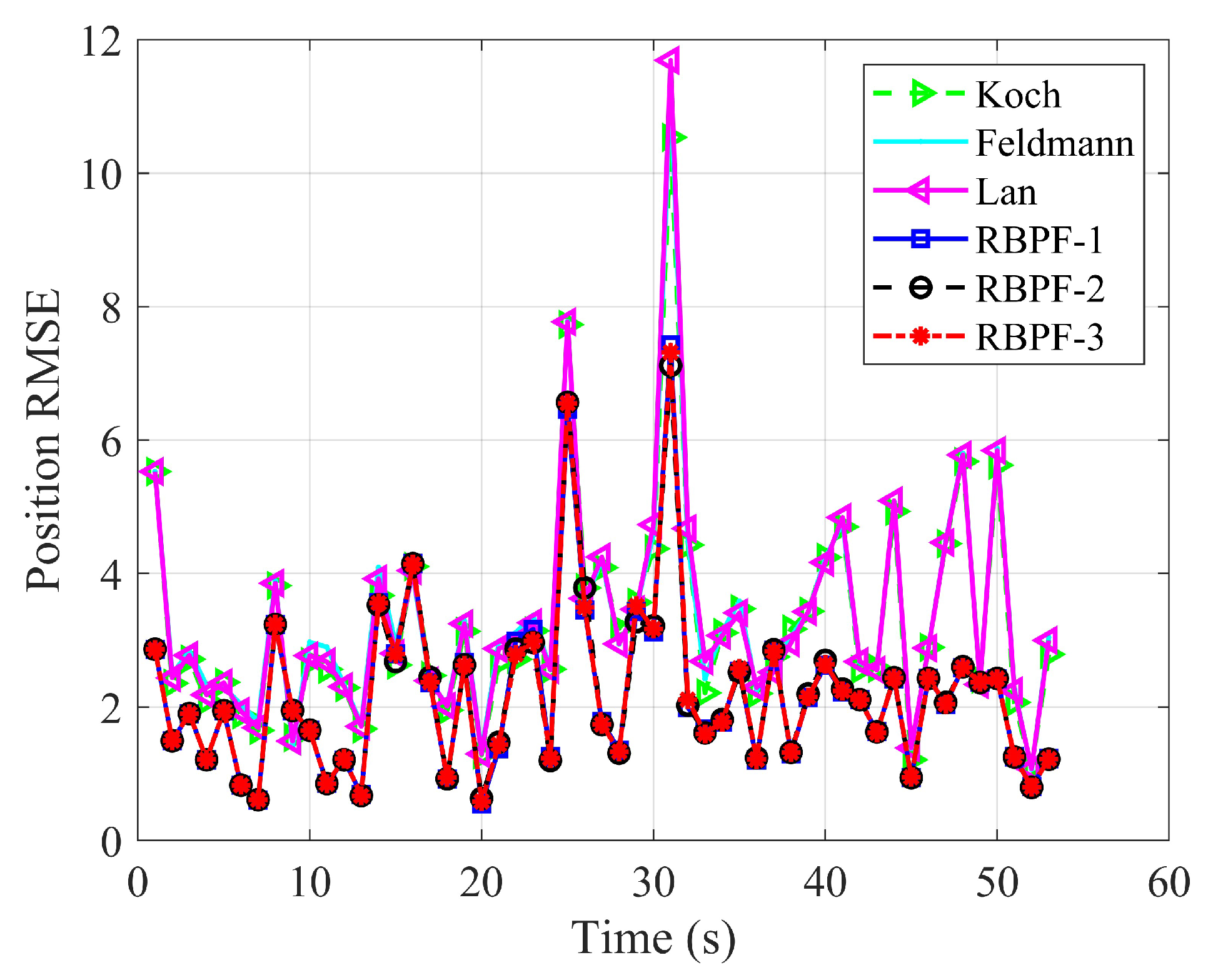
4. Experimental Results and Analysis

The digital staring radar system designed in this study operates in the S-band, as shown in Figure 1. The digital staring radar featuring a wide transmission beam and lower gain, enhances detection performance by coherently accumulating echo energy from scattering points, thereby improving the signal-to-noise ratio.
We conduct cluster target tracking simulation experiments under different scenarios to evaluate the proposed tracking algorithms. The tracking accuracy performance is compared against the Koch method, the Feldmann method, and the Lan method, demonstrating the effectiveness and robustness of our approach. The root mean square error (RMSE) is adopted as the evaluation criterion to quantitatively assess the performance of the algorithms tested. It is calculated using the follow formula:
RMSE k = 1 N r i = 1 N r x k x ^ k T x k x ^ k ,
where x k and x ^ k are the real value and the estimated value of the cluster targets, N r is the number of totaling runs. The RMSEs of both cluster position and velocity are respectively considered in the following simulation experiments of two scenarios.

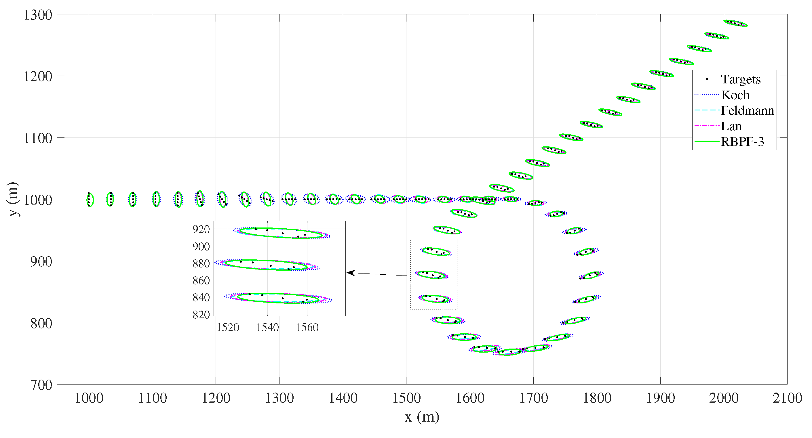
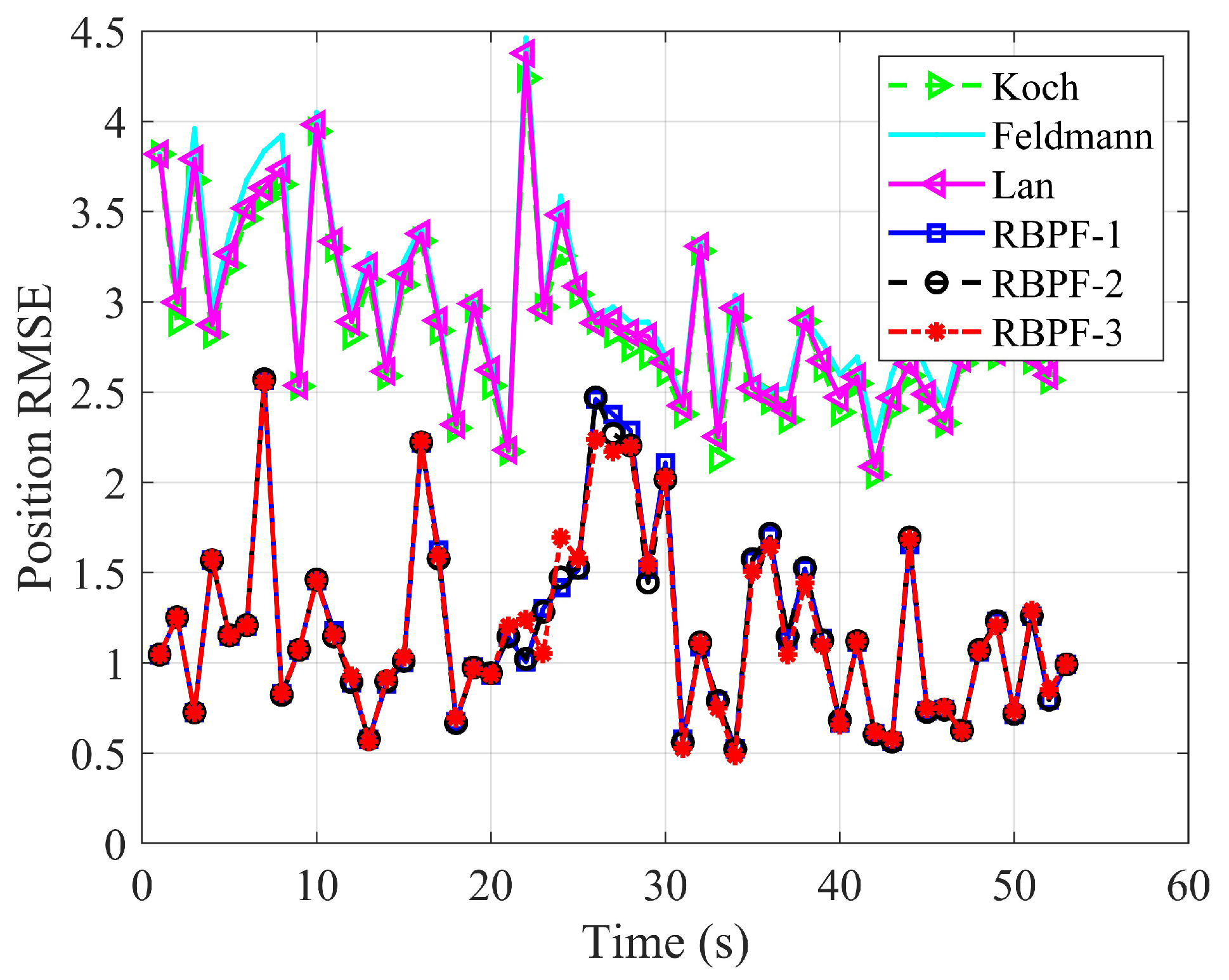
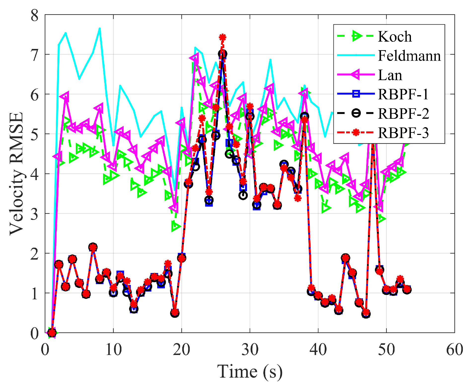
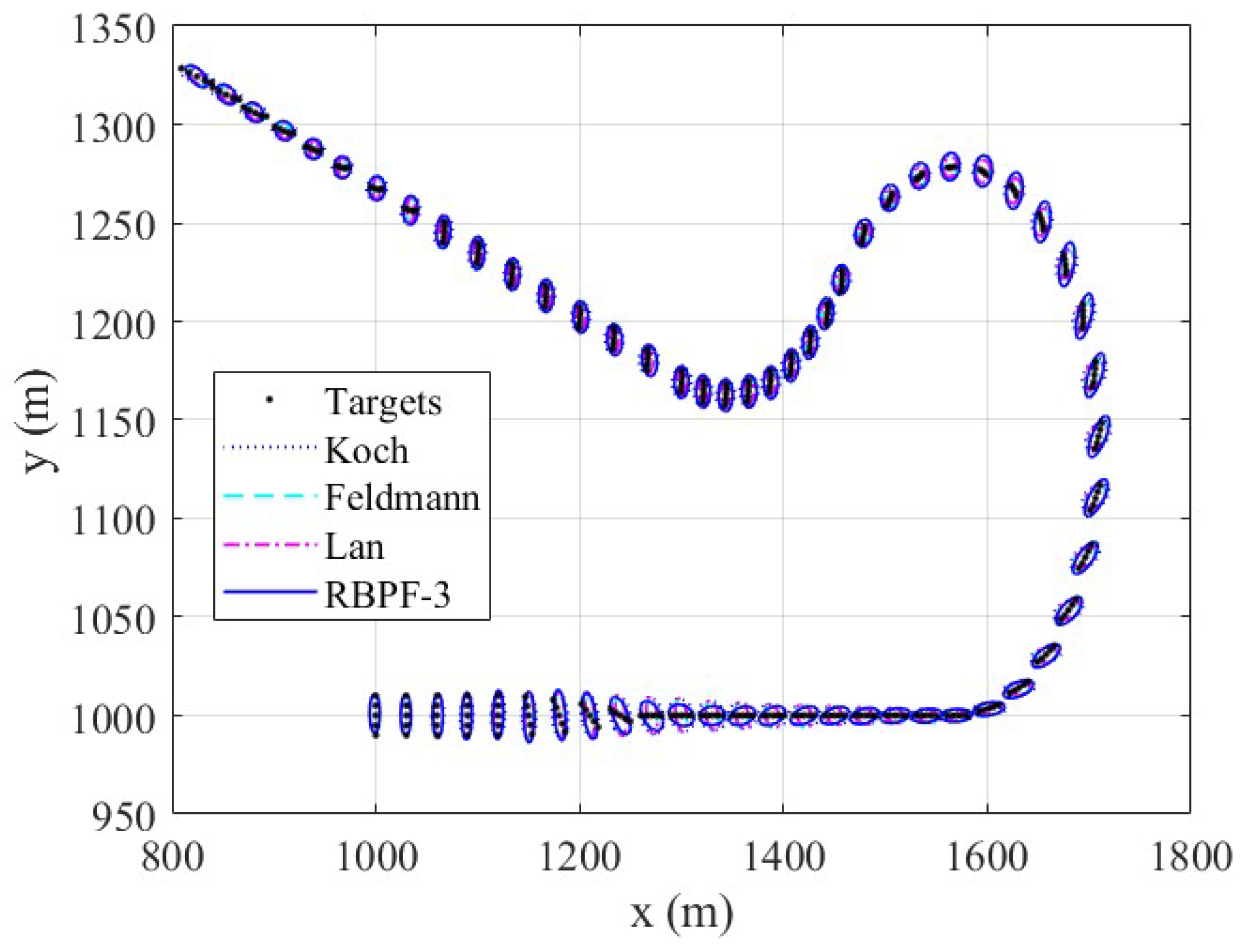
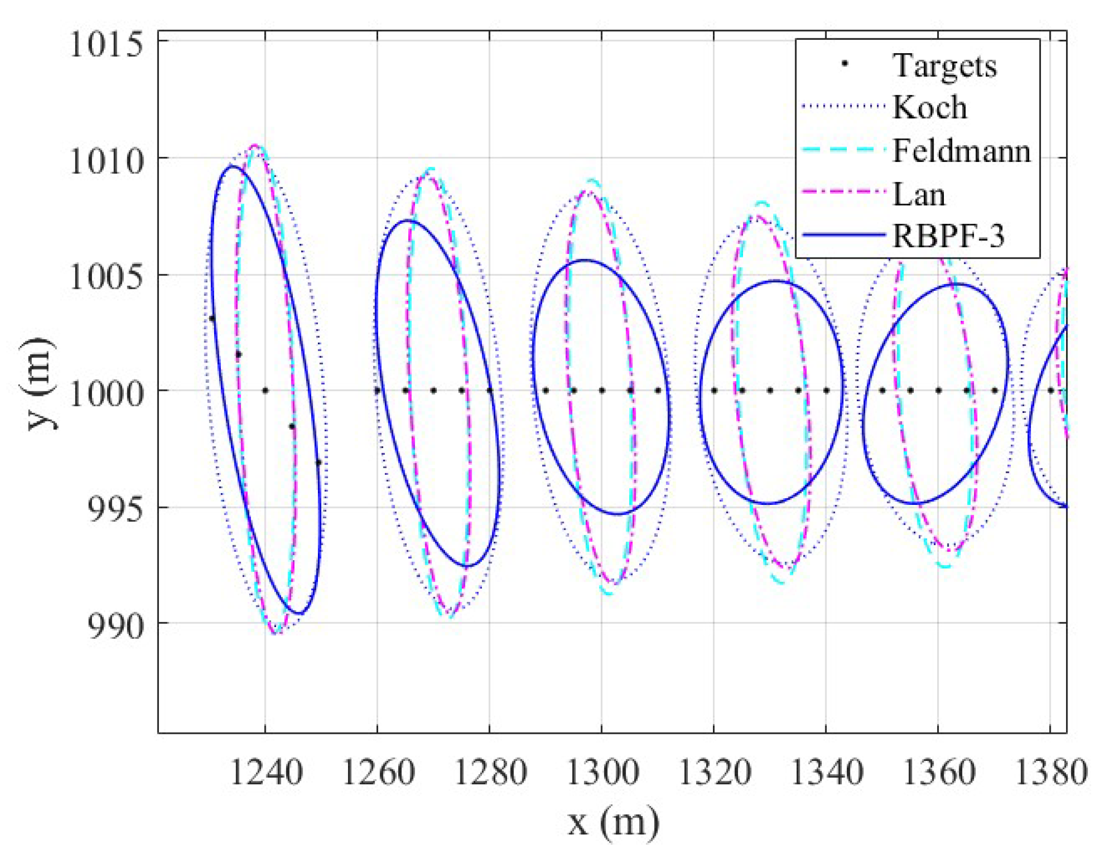
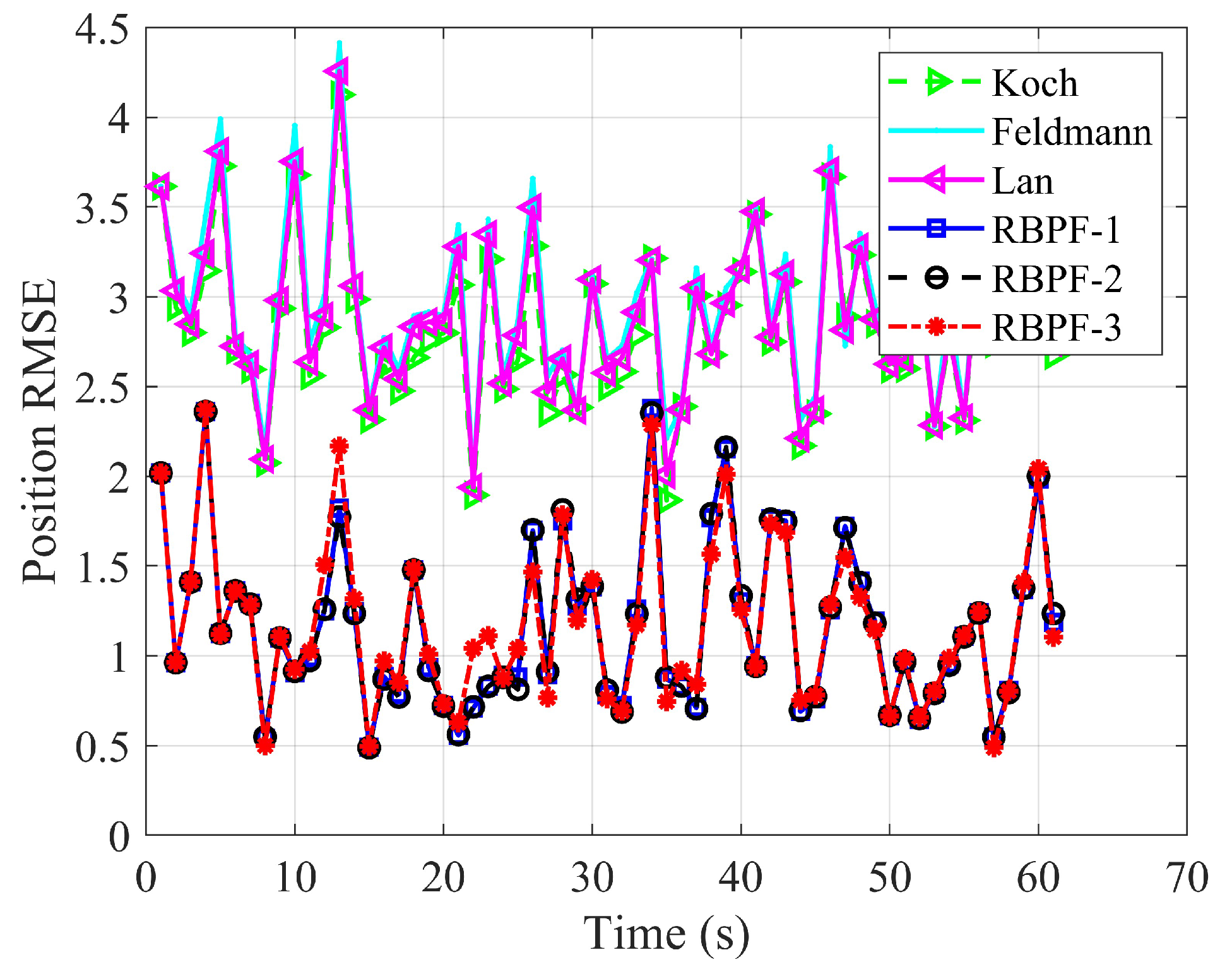
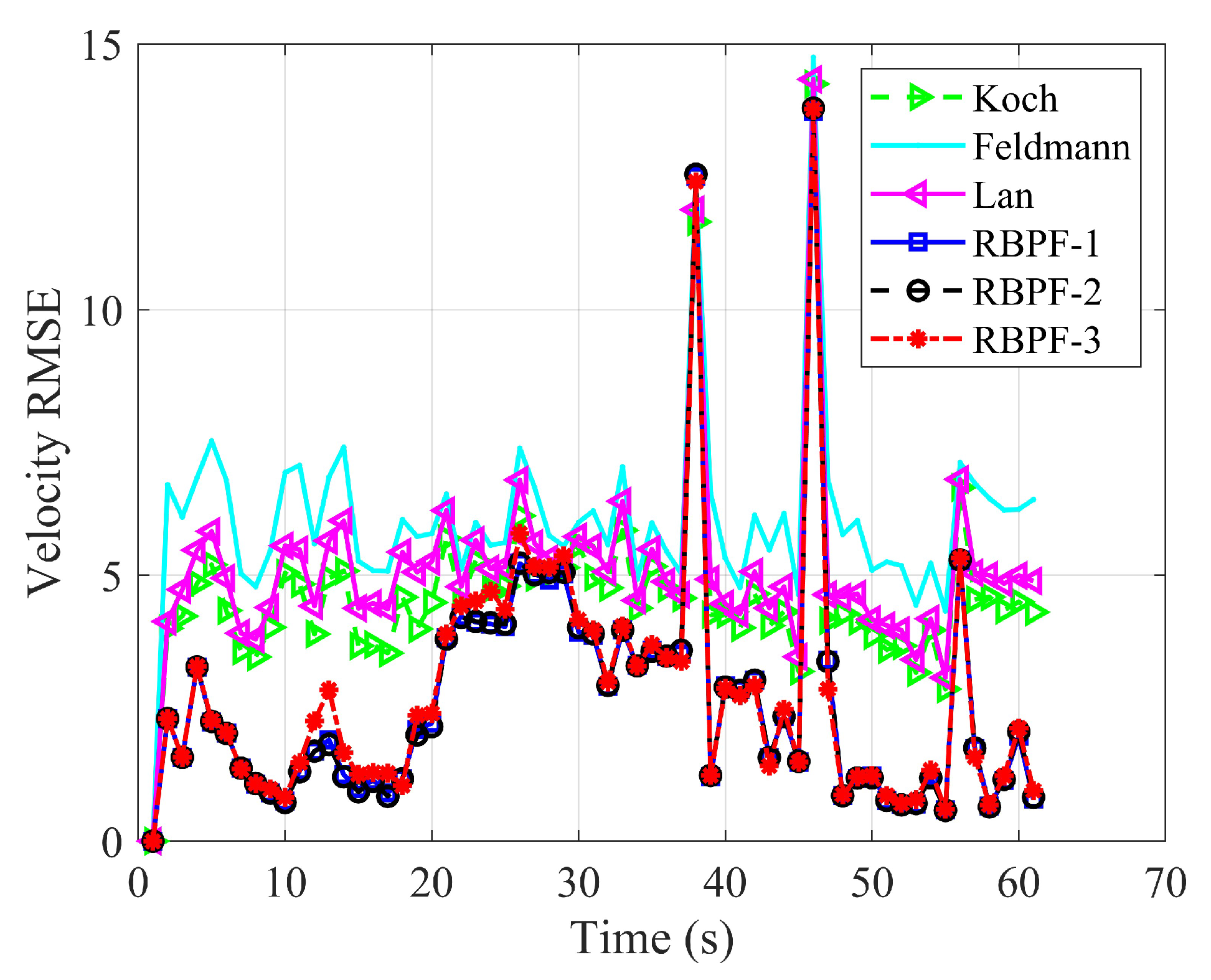
4.1. Cluster Target Tracking Test Experiment of Scenario One

Simulation scenario one: We simulate a formation of 5 individual targets flying with constant speed, 35 m/s, in the ( x , y )-plane, the interval between two adjacent targets is set to 5 m; After flying for 19 s, the cluster targets change their formation and move clockwise for 18 s; Finally, they keep the formation and fly in a straight line under constant speed 35 m/s for 15 s. The flying trajectory of the cluster is shown in Figure 2, in which the black solid circle means the real target.
We tested the RBPF with basic resampling method (marked as RBPF-1 in subsequent sections for short), RBPF using Resampling with Particles Grid Segmentation method (marked as RBPF-2 for short), RBPF using Resampling with Particles Segmentation Cross Summation method (marked as RBPF-3), and the compared Koch method, Feldmann method and Lan method. Each cluster target tracking simulation run of the tested methods is repeated 5 times, the target tracking results including targets’ position and velocity, and extended parameter values are estimated; The tracking accuracy results RMSE is calculated and listed in Table 2. When calculating the RMSE, we use the position and velocity of the central target of the cluster to form the real state. The cluster target tracking trajectories of Koch method, Feldmann method, Lan method and RBPF-3 are shown in Figure 2. We can see that the achieved green elliptic curves of RBPF-3 cover the cluster targets with proper scale size, and rotated with the adjustable cluster target formation. The elliptic curves cover all of the targets in a cluster, but with smaller size, reveals the good performance of presented RBPF-3 among the compared methods. In Table 2, the mean values of position/velocity RMSE of tracking targets of presented RBPF-2 and RBPF-3 are smaller than the other compared methods. Figure 3 and Figure 4 also show that the position/velocity RMSE results of the tested RBPF-2 and RBPF-3 methods are better in most situations.

4.2. Cluster Target Tracking Test Experiment of Scenario Two

Simulation scenario two: We simulate a formation of 5 individual targets flying with constant speed, 30 m/s, in the ( x , y )-plane, the interval between two adjacent targets is set to 5 m; After flying for 19 s, the UAV cluster targets change their formation and move counterclockwise for 18 s; Then, they keep the formation and fly in a straight line under constant speed 35 m/s for 10 s; Finally, targets move in a straight line direction with various speeds for 5 s. The flying trajectory of the cluster is shown in Figure 5, in which the black solid circle is the real target.
We tested the RBPF-1, RBPF-2, RBPF-3 (using the turn rate parameter), Koch method, Feldmann method and Lan method using the dataset of achieved in scenario two. Each cluster target tracking simulation run of the tested methods is repeated 20 times, the target tracking results including targets’ position and velocity, and extended parameter values are estimated; The tracking accuracy results RMSE is calculated and listed in Table 3. In Table 3, the mean values of position/velocity RMSE of tracking targets of presented RBPF-2 and RBPF-3 are smaller than the Koch, Feldmann and Lan methods.
We use the position and velocity of the central target of the cluster to form the real state to calculate the RMSE results. The cluster target tracking trajectories of Koch method, Feldmann method, Lan method and RBPF-3 are shown in Figure 5. We can see that the achieved green elliptic curves of RBPF-3 cover the cluster targets with small scale size, and rotated with the adjustable cluster target formation quickly. The elliptic curves cover the targets well, and reveals the good performance of presented RBPF-3. Figure 6 and Figure 7 show that the position/velocity RMSE results of the tested RBPF-2 and RBPF-3 methods are better.

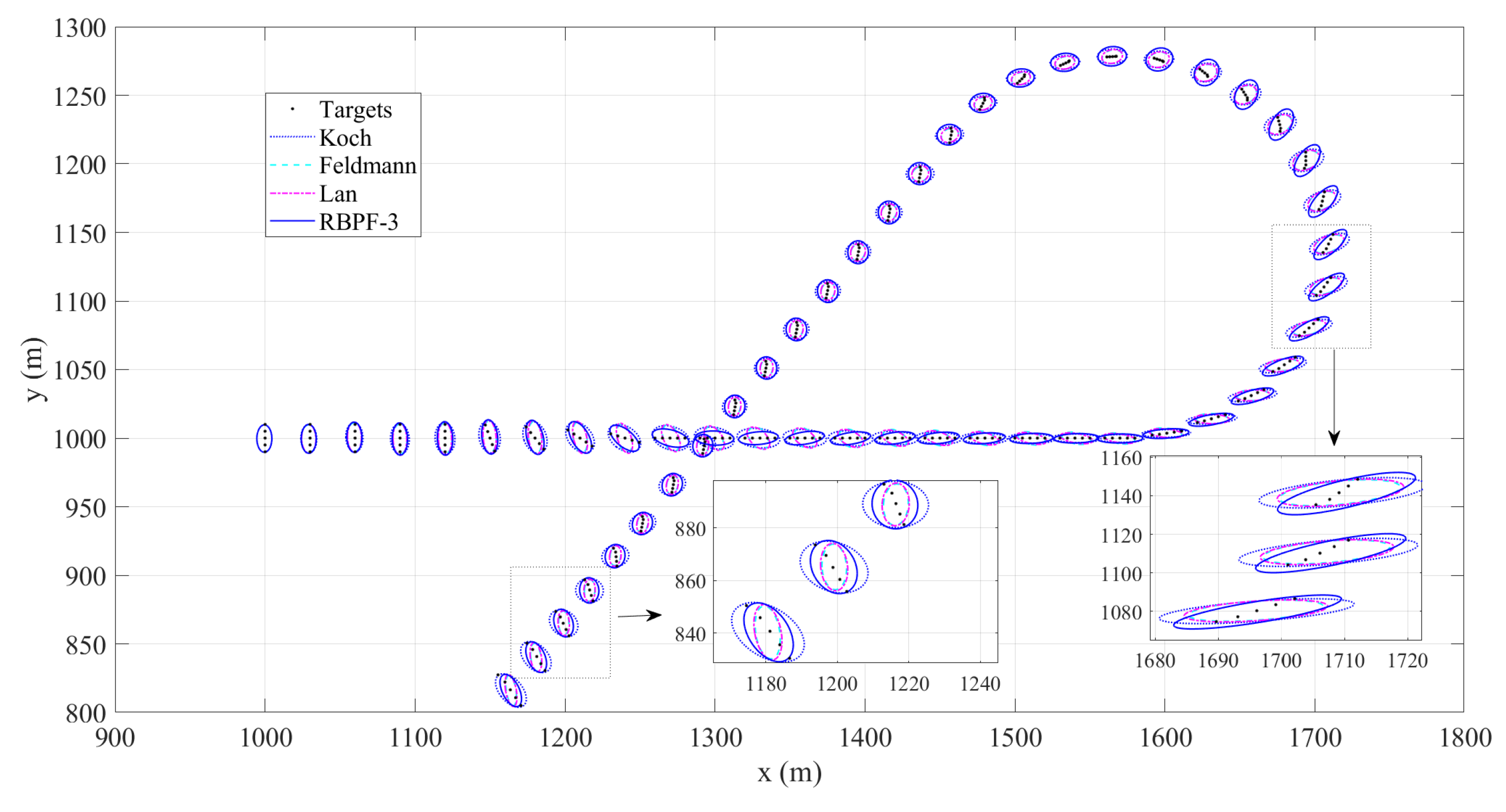
4.3. Cluster Target Tracking Test Experiment of Scenario Three

Simulation scenario three: We simulate a formation of 5 individual targets flying with constant speed, 30 m/s, in the ( x , y )-plane, the interval between two adjacent targets is set to 5 m; After flying for 19 s, the UAV cluster targets change their formation and move counter-clockwise for 18 s; Then, they change their direction and velocity and keep on flying for 8 s. After that, they keep the formation and fly in a straight line under constant speed 35 m/s for 10 s; Finally, targets move in a straight line direction with various speeds for 5 s. The flying trajectory of the cluster is shown in Figure 8 and Figure 9, in which the black solid circle is the real target.
We tested the RBPF-1, RBPF-2, RBPF-3 (using the turn rate parameter), Koch method, Feldmann method and Lan method using the dataset of achieved in scenario three. Each cluster target tracking simulation run of the tested methods is repeated 20 times, the target tracking results including targets’ position and velocity, and extended parameter values are estimated. We use the position and velocity of the central target of the cluster to form the real state to calculate the RMSE results. The cluster target tracking trajectories of Koch method, Feldmann method, Lan method and RBPF-3 are shown in Figure 8 and Figure 9. We can see that the achieved green elliptic curves of RBPF-3 cover the cluster targets with small scale size, and rotated with the adjustable cluster target formation quickly. The elliptic curves cover the targets well, and shows the good performance of presented RBPF-3. Figure 10 and Figure 11 show that the position/velocity RMSE results of the tested RBPF-1, RBPF-2 and RBPF-3 methods are better.
The simulation results demonstrate the effectiveness of the proposed improved random matrix and Rao-Blackwellized particle filter algorithm to track the target of the UAV cluster.

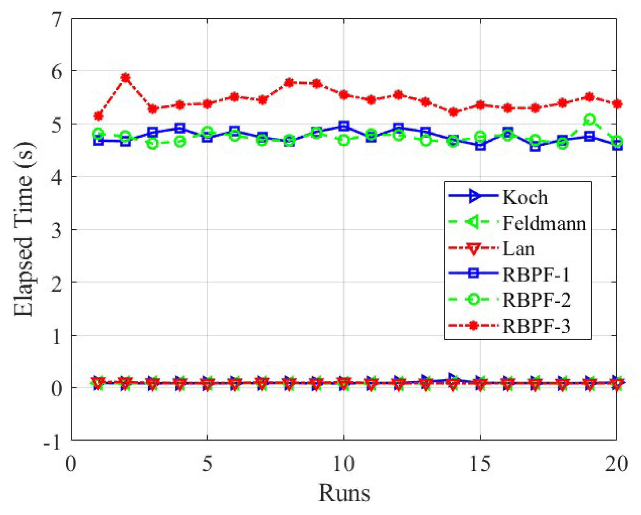
4.4. Computational Complexity Test

To analyze the computational complexity of the researched methods, simulation experiments were implemented using a laptop of Intel(R) Core(TM) i7 2.30 GHz and RAM 32 GB. Each simulation experiment using the compared methods is repeat 20 times, and each method implemented the target estimation about 60 s. The elapsed time results of each run for cluster target tracking using the compared methods in scenario three are recorded and shown in Figure 12. The average elapsed time of Koch, Feldmann, Lan, RBPF-1, RBPF-2, and RBPF-3 in each run is 0.0886 s, 0.0824 s, 0.0882 s, 4.7556 s, 4.7428 s, and 5.4421 s, respectively, which indicates that the computational complexity of the presented methods is higher than the Koch, Feldmann, and Lan methods. Since the average elapsed time for the target estimation in each second is smaller than 1 when using the presented methods, the RBPF-1, RBPF-2, and RBPF-3 satisfy the time performance required. Compared with the Koch, Feldmann, and Lan methods, the presented method will require more computational resources during the real-world deployment.

5. Conclusions

An adaptive random matrix approach for tracking UAV swarms is integrated into a designed digital staring radar system in this study. In the tracking approaches for UAVs cluster targets, most existing models and methods assume that the extended ellipses of cluster targets remain approximately invariant and do not consider the complex variation processes, such as the rotation of the extended ellipses. This paper proposes the introduction of additional extension parameters to represent the intricate variation processes of the extended state to address this limitation. It employs a sequential Monte Carlo method to approximate the posterior estimation of both the motion state and the extension state. An adaptive Rao-Blackwellized Particle Filter with improved resampling with particles segmentation cross summation, is then employed to estimate the motion and extension states of the UAV swarm jointly. Multiple test experiments were conducted. Based on the simulation results, it is evident that the proposed method can swiftly respond to changes in target extension, particularly when rotation occurs. Furthermore, it ensures an estimation accuracy of the motion state that is comparable to the compared methods.

Author Contributions

Conceptualization, N.Z., F.Z. and X.L.; methodology, N.Z., F.Z. and Y.Z.; software, N.Z.; validation, N.Z., F.Z. and H.X.; investigation, N.Z. and Y.Z.; data curation, N.Z. and F.Z.; writing original draft preparation, N.Z., G.N., and X.L.; writing review and editing, N.Z., Y.Z., G.N., and F.Z.; supervision, Y.Z. and H.X. All authors contributed to writing the final manuscript. All authors have read and agreed to the published version of the manuscript.

Funding

This work is supported by the National Natural Science Foundation of China (Grant No. 62102466), the Fundamental Research Funds for the Central Universities, Sun Yat-sen University (Grant No. 24qnpy164), Guangdong Basic and Applied Basic Research Foundation Grant (No. 2022A1515140103 and No. 2023A1515011588), the Shenzhen Science and Technology Program (grant No. 202206193000001, 20220815171723002 and grant No. JCYJ20240813151238049), and the Open Fund of the State Key Laboratory of Satellite Navigation Systems and Equipment Technology (Grant No. CEPNT2023B08).

Data Availability Statement

All data that support the findings of this study are included within the article.

Acknowledgments

We would like to extend our sincere gratitude to Shiyou Xu for his invaluable contributions to the exploration and verification of this research, and Xiaoyan Lv for her helpful discussions and comments.

Conflicts of Interest

The authors declare no conflicts of interest.

References

  1. Wen, L.; Zhen, Z.; Tao, C.; Ding, J. Distributed Cooperative Strategy of UAV Swarm Without Speed Measurement Under Saturation Attack Mission. IEEE Trans. Aerosp. Electron. Syst. 2024, 60, 4518–4529. [Google Scholar]
  2. Lei, Y.; Tong, X.; Qiu, C.; Sun, Y.; Tang, J.; Guo, C.; Li, H. Onboard Data Management Approach Based on a Discrete Grid System for Multi-UAV Cooperative Image Localization. IEEE Trans. Geosci. Remote Sens. 2023, 61, 1–17. [Google Scholar]
  3. Ye, X.; Xue, W.; Chen, X.; Zhang, Y.; Wang, X.; Guan, J. Cauchy Kernel-Based AEKF for UAV Target Tracking via Digital Ubiquitous Radar Under the Sea–Air Background. IEEE Geosci. Remote Sens. Lett. 2024, 21, 1–5. [Google Scholar]
  4. Sun, Z.; Hu, C.; Cui, K.; Wang, R.; Ding, M.; Yan, Z.; Wu, D. Extracting Bird and Insect Migration Echoes From Single-Polarization Weather Radar Data Using Semi-Supervised Learning. IEEE Trans. Geosci. Remote Sens. 2024, 62, 1–12. [Google Scholar]
  5. Sayed, A.N.; Ramahi, O.M.; Shaker, G. In the Realm of Aerial Deception: UAV Classification via ISAR Images and Radar Digital Twins for Enhanced Security. IEEE Sens. Lett. 2024, 8, 1–4. [Google Scholar]
  6. Yuan, D.; Zhang, H.; Shu, X.; Liu, Q.; Chang, X.; He, Z.; Shi, G. Thermal Infrared Target Tracking: A Comprehensive Review. IEEE Trans. Instrum. Meas. 2024, 73, 1–19. [Google Scholar]
  7. Chen, Y.; Li, Z.; Wu, L.; Chen, P. An Efficient Multi-Object Tracking Guided by Spatial Clustering on Vision Sensors. IEEE Sens. J. 2024, 24, 19344–19351. [Google Scholar]
  8. Zhu, N.; Xi, Z.; Wu, C.; Zhong, F.; Qi, R.; Chen, H. Inductive Conformal Prediction Enhanced LSTM-SNN Network: Applications to Birds and UAVs Recognition. IEEE Geosci. Remote Sens. Lett. 2024, 21, 1–5. [Google Scholar]
  9. Liu, Z.; Wang, Z.K.; Yang, Y.B.; Lu, Y. A Data-Driven Maneuvering Target Tracking Method Aided with Partial Models. IEEE Trans. Veh. Technol. 2024, 73, 414–425. [Google Scholar]
  10. Ming, R.; Zhou, Z.; Luo, X.; Liu, W.; Le, Z.; Song, C.; Jiang, R.; Zang, Y. Optical Tracking System for Multi-UAV Clustering. IEEE Sens. J. 2021, 21, 19382–19394. [Google Scholar]
  11. Liang, T.; Zhang, T.; Yang, J.; Feng, D.; Zhang, Q. UAV-Aided Positioning Systems for Ground Devices: Fundamental Limits and Algorithms. IEEE Internet Things J. 2022, 9, 13470–13485. [Google Scholar] [CrossRef]
  12. Ye, T.; Qin, W.; Li, Y.; Wang, S.; Zhang, J.; Zhao, Z. Dense and Small Object Detection in UAV-Vision Based on a Global-Local Feature Enhanced Network. IEEE Trans. Instrum. Meas. 2022, 71, 1–13. [Google Scholar] [CrossRef]
  13. Zhu, N.; Xu, S.; Li, C.; Hu, J.; Fan, X.; Wu, W.; Chen, Z. An Improved Phase-Derived Range Method Based on High-Order Multi-Frame Track-Before-Detect for Warhead Detection. Remote Sens. 2022, 14, 29. [Google Scholar] [CrossRef]
  14. Song, Q.; Huang, S.; Zhang, Y.; Chen, X.; Chen, Z.; Zhou, X.; Deng, Z. Radar Target Classification Using Enhanced Doppler Spectrograms with ResNet34_CA in Ubiquitous Radar. Remote Sens. 2024, 16, 2860. [Google Scholar] [CrossRef]
  15. Chen, X.; Zhang, H.; Song, J.; Guan, J.; Li, J.; He, Z. Micro-Motion Classification of Flying Bird and Rotor Drones via Data Augmentation and Modified Multi-Scale CNN. Remote Sens. 2022, 14, 1107. [Google Scholar] [CrossRef]
  16. Zhu, N.; Xi, Z.; Chen, H.; Xu, S.; Wang, Y.; Zhong, F. Mondrian Conformal Prediction Enhanced LSTM for Birds and Drones Recognition. In IET Conference Proceedings CP874 2023; The Institution of Engineering and Technology: Stevenage, UK, 2023; pp. 760–765. [Google Scholar]
  17. Zhao, Y.; Su, Y. Synchrosqueezing Phase Analysis on Micro-Doppler Parameters for Small UAVs Identification with Multichannel Radar. IEEE Geosci. Remote. Sens. Lett. 2020, 17, 411–415. [Google Scholar] [CrossRef]
  18. Yu, X.; Wei, S.; Fang, Y.; Sheng, J.; Zhang, L. Low-Altitude Slow Small Target Threat Assessment Algorithm by Exploiting Sequential Multi-Feature with Long-Short-Term-Memory. IEEE Sens. J. 2023, 23, 21524–21533. [Google Scholar] [CrossRef]
  19. Kang, K.B.; Choi, J.H.; Cho, B.L.; Lee, J.S.; Kim, K.T. Analysis of Micro-Doppler Signatures of Small UAVs Based on Doppler Spectrum. IEEE Trans. Aerosp. Electron. Syst. 2021, 57, 3252–3267. [Google Scholar] [CrossRef]
  20. Chen, X.; Guan, J.; Chen, W.; Zhang, L.; Yu, X. Sparse Long-Time Coherent Integration-Based Detection Method for Radar Low-Observable Manoeuvring Target. IET Radar Sonar Navig. 2020, 14, 538–546. [Google Scholar] [CrossRef]
  21. White, D.; Jahangir, M.; Baker, C.J.; Antoniou, M. Urban Bird-Drone Classification with Synthetic Micro-Doppler Spectrograms. IEEE Trans. Radar Syst. 2024, 2, 167–179. [Google Scholar] [CrossRef]
  22. Chen, Z.; Ji, H.; Zhang, Y.; Zhu, Z.; Li, Y. High-Resolution Feature Pyramid Network for Small Object Detection on Drone View. IEEE Trans. Circuits Syst. Video Technol. 2023, 34, 475–489. [Google Scholar] [CrossRef]
  23. Zheng, Y.; Chen, Z.; Lv, D.; Li, Z.; Lan, Z.; Zhao, S. Air-to-Air Visual Detection of Micro-UAVs: An Experimental Evaluation of Deep Learning. IEEE Robot. Autom. Lett. 2021, 6, 1020–1027. [Google Scholar]
  24. Zhao, Y.; Su, Y. The Extraction of Micro-Doppler Signal with EMD Algorithm for Radar-Based Small UAVs’ Detection. IEEE Trans. Instrum. Meas. 2020, 69, 929–940. [Google Scholar]
  25. Dugger, K. Techniques for Wildlife Investigations and Management. Condor 2007, 109, 981–983. [Google Scholar]
  26. Zhu, N.; Hu, J.; Xu, S.; Wu, W.; Zhang, Y.; Chen, Z. Micro-Motion Parameter Extraction for Ballistic Missile with Wideband Radar Using Improved Ensemble EMD Method. Remote Sens. 2021, 13, 3545. [Google Scholar] [CrossRef]
  27. Drummond, O.E.; Society of Photo-Optical Instrumentation Engineers; CREOL (Research center); SPIE Technical Symposium on Optical Engineering and Photonics in Aerospace Sensing. Signal and Data Processing of Small Targets 1990 : 16–18 April 1990, Orlando, Florida / Oliver E. Drummond, Chair/Editor; Sponsored by SPIE--The International Society for Optical Engineering; Cooperative Organization, CREOL/University of Central Florida; Society of Photo-Optical Instrumentation Engineers: Bellingham, WA, USA, 1990; Volume 1305. [Google Scholar]
  28. Koch, J.W. Bayesian Approach to Extended Object and Cluster Tracking Using Random Matrices. IEEE Trans. Aerosp. Electron. Syst. 2008, 44, 1042–1059. [Google Scholar]
  29. Gupta, A.K.; Nagar, D.K. Matrix Variate Distributions; CRC Press: Boca Raton, FL, USA, 2020; pp. 13–26. [Google Scholar]
  30. Feldmann, M.; Fränken, D.; Koch, W. Tracking of Extended Objects and Group Targets Using Random Matrices. IEEE Trans. Signal Process. 2010, 59, 1409–1420. [Google Scholar]
  31. Orguner, U. A Variational Measurement Update for Extended Target Tracking with Random Matrices. IEEE Trans. Signal Process. 2012, 60, 3827–3834. [Google Scholar] [CrossRef]
  32. Bishop, C.M. Pattern Recognition and Machine Learning; Springer: Berlin/Heidelberg, Germany, 2006. [Google Scholar]
  33. Lan, J.; Li, X.R. Tracking of Extended Object or Target Group Using Random Matrix: New Model and Approach. IEEE Trans. Aerosp. Electron. Syst. 2016, 52, 2973–2989. [Google Scholar]
  34. Lan, J.; Li, X.R. Extended-object or Group-Target Tracking Using Random Matrix with Nonlinear Measurements. IEEE Trans. Signal Process. 2019, 67, 5130–5142. [Google Scholar]
  35. Mo, L.; Song, X.; Zhou, Y.; Sun, Z.K. Unbiased Converted Measurements for Tracking. IEEE Trans. Aerosp. Electron. Syst. 1998, 34, 1023–1027. [Google Scholar]
  36. Duan, Z.; Han, C.; Li, X.R. Comments on Unbiased Converted Measurements for Tracking. IEEE Trans. Aerosp. Electron. Syst. 2004, 40, 1374. [Google Scholar]
  37. Granström, K.; Natale, A.; Braca, P.; Ludeno, G.; Serafino, F. Gamma Gaussian Inverse Wishart Probability Hypothesis Density for Extended Target Tracking Using X-Band Marine Radar Data. IEEE Trans. Geosci. Remote Sens. 2015, 53, 6617–6631. [Google Scholar]
  38. Doucet, A.; Godsill, S.; Andrieu, C. On Sequential Monte Carlo Sampling Methods for Bayesian Filtering. Stat. Comput. 2000, 10, 197–208. [Google Scholar]
  39. Mustiere, F.; Bolic, M.; Bouchard, M. Rao-Blackwellised Particle Filters: Examples of Applications. In Proceedings of the 2006 Canadian Conference on Electrical and Computer Engineering, Ottawa, ON, Canada, 7–10 May 2006; pp. 1196–1200. [Google Scholar]
  40. Cheng, L.; Sengupta, A.; Cao, S. Deep Learning-Based Robust Multi-Object Tracking via Fusion of mmWave Radar and Camera Sensors. IEEE Trans. Intell. Transp. Syst. 2024, 25, 17218–17233. [Google Scholar]
  41. Huang, Y.; Guo, R.; Zhang, Y.; Chen, Z. Deep-Reinforcement-Learning-Based Radar Parameter Adaptation for Multiple-Target Tracking. IEEE Trans. Aerosp. Electron. Syst. 2024, 60, 7125–7141. [Google Scholar]
  42. Zhang, H.; Chen, H.; Zhang, W.; Zhang, X. Trajectory Planning for Airborne Radar in Extended Target Tracking Based on Deep Reinforcement Learning. Digit. Signal Process. 2024, 153, 104603. [Google Scholar]
  43. Cramér, H. Mathematical Methods of Statistics (PMS-9), Volume 9; Princeton University Press: Princeton, NJ, USA, 2016. [Google Scholar]
  44. Chen, R.; Liu, J.S. Mixture Kalman Filters. J. R. Stat. Soc. B 2000, 62, 493–508. [Google Scholar]
  45. Arulampalam, M.S.; Maskell, S.; Gordon, N.; Clapp, T. A Tutorial on Particle Filters for Online Nonlinear/Non-Gaussian Bayesian Tracking. IEEE Trans. Signal Process. 2002, 50, 2. [Google Scholar]
Figure 1. Holographic staring radar sensor application scenarios.
Remotesensing 17 01172 g001
Figure 2. Cluster target tracking trajectory of compared methods in scenario one.
Remotesensing 17 01172 g002
Figure 3. Cluster target tracking RMSE of position of compared methods in scenario one.
Remotesensing 17 01172 g003
Figure 4. Cluster target tracking RMSE of velocity of compared methods in scenario one.
Remotesensing 17 01172 g004
Figure 5. Cluster target tracking trajectory of compared methods in scenario two.
Remotesensing 17 01172 g005
Figure 6. Cluster target tracking RMSE of position of compared methods in scenario two.
Remotesensing 17 01172 g006
Figure 7. Cluster target tracking RMSE of velocity of compared methods in scenario two.
Remotesensing 17 01172 g007
Figure 8. Cluster target tracking trajectory of compared methods in scenario three (full).
Remotesensing 17 01172 g008
Figure 9. Cluster target tracking trajectory of compared methods in scenario three (partially magnified).
Remotesensing 17 01172 g009
Figure 10. Cluster target tracking RMSE of position of compared methods in scenario three.
Remotesensing 17 01172 g010
Figure 11. Cluster target tracking RMSE of velocity of compared methods in scenario three.
Remotesensing 17 01172 g011
Figure 12. Cluster target tracking Elapsed time of compared methods in scenario three.
Remotesensing 17 01172 g012
Table 1. The process of the proposed algorithm.
(1) Initialization
Initialize Kalman filter
       x ^ 0 | 0 i = E x 0 , P 0 | 0 i = E x 0 E x 0 x 0 E x 0 T
Initialize particles filter
       X 0 i = E 0 i , w 0 i p X 0 = p E 0 p w 0
(2) Recursion
Prediction
      Sequential sampling of particles
          X k i = E k i , φ k i p E k | E k 1 i , φ k 1 i p φ k | φ k 1 i
      One step prediction of motion state and covariance
          x ^ k | k 1 i = F k x ^ k 1 | k 1 i
          P k | k 1 i = F k 1 P k 1 | k 1 i F k 1 T + E k i D k
Update
      Update particle weights
          w k i p Z k | X 0 : k i , Z 1 : k 1 w k 1 i
      Update state of motion
          S k i = H k P k | k 1 i H k T + ( α E k i + R k ) / n k
          K k i = P k | k 1 i H k T S k i 1
          x ^ k | k i = x ^ k | k 1 i + K k i ( z ¯ k H k x ^ k | k 1 i )
          P k k i = P k k 1 i K k S k i K k i T
      Normalized weights
          w k i = w k i / i = 1 N s w k i
      Resampling
         Calculate the effective number of particles, and if N eff < N th ,
         perform the resampling step.
      Compute the posterior estimate of the joint state.
          x ^ k | k = E x k | Z 1 : k i = 1 N s w k i x ^ k | k i ,
          E ^ k | k = E E k | Z 1 : k i = 1 N s w k i E k i
Table 2. Cluster target tracking results (RMSE) in scenario one. (Pos means position (units: m), Vel means velocity (units: m/s), STD means the standard deviation).
MethodsMean (Pos (m))STD (Pos (m))Mean (Vel (m/s))STD (Vel (m/s))
Koch3.26021.63635.62342.3776
Feldmann3.35791.70176.49332.4439
Lan3.33941.74616.27692.7961
RBPF-12.18641.28694.13252.8612
RBPF-22.18491.26934.10882.8326
RBPF-32.18461.28134.12072.8421
Table 3. Cluster target tracking results (RMSE) in scenario two. (Pos means position (units: m), Vel means velocity (units: m/s), STD means the standard deviation).
MethodsMean (Pos (m))STD (Pos (m))Mean (Vel (m/s))STD (Vel (m/s))
Koch2.87680.48764.36381.0702
Feldmann3.01290.51225.75701.1808
Lan2.92820.49924.78491.0896
RBPF-11.20300.51862.29701.6809
RBPF-21.19920.50902.28741.6700
RBPF-31.19560.49702.39141.7595
Disclaimer/Publisher’s Note: The statements, opinions and data contained in all publications are solely those of the individual author(s) and contributor(s) and not of MDPI and/or the editor(s). MDPI and/or the editor(s) disclaim responsibility for any injury to people or property resulting from any ideas, methods, instructions or products referred to in the content.

