UOrtos: Methodology for Co-Registration and Subpixel Georeferencing of Satellite Imagery for Coastal Monitoring

Abstract

This study introduces a novel methodology for the automated co-registration and georeferencing of satellite imagery to enhance the accuracy of shoreline detection and coastal monitoring. The approach utilizes feature-based methods, cross-correlation, and RANSAC (RANdom SAmple Consensus) algorithms to accurately align images while avoiding outliers. By collectively analyzing the entire set of images and clustering them based on their pixel-pair connections, the method ensures robust transformations across the dataset. The methodology is applied to Sentinel-2 and Landsat images across four coastal sites (Duck, Narrabeen, Torrey Pines, and Truc Vert) from January 2020 to December 2023. The results show that the proposed approach effectively reduces the errors from ∼1 to at least $0.4$ px (although they are likely below $0.2$ px). This approach can enhance the precision of existing algorithms for coastal feature tracking, such as shoreline detection, and aids in differentiating georeferencing errors from the actual impacts of storms or beach nourishment activities. The tool can also handle complex cases of significant image rotation due to varied projections. The findings emphasize the importance of co-registration for reliable shoreline monitoring, with potential applications in coastal management and climate change impact studies.

1. Introduction

Understanding coastal dynamics is crucial for numerous environmental, scientific, and socioeconomic reasons. Coastal regions are among the most dynamic and vulnerable landscapes on Earth, experiencing continuous changes influenced by natural processes such as erosion and sedimentation, as well as human activities such as urbanization and infrastructure development. Furthermore, climate change-induced sea level rise is expected to increasingly act as a significant forcing mechanism in shaping these regions [1]. These dynamics not only impact coastal ecosystems and biodiversity but also pose significant risks to coastal communities, economies, and infrastructures. Monitoring and analyzing coastal dynamics using satellite imagery provides essential insights into these processes, helping to manage effective coastal zones, prepare for disasters, adapt to climate change, and plan sustainable development. Therefore, comprehensive studies on satellite shoreline detection play a pivotal role in advancing our understanding and management of coastal environments worldwide. Provided the present global trend in coastal erosion, which could be enhanced by sea level rise and more frequent extreme events under a changing climate [1], the socioeconomical interest of the coastal region and the increasing availability of satellite data, it comes as no surprise that the interest of the scientific community on this topic has grown rapidly in the last years [2].

Recent advancements in satellite technologies have revolutionized the field of Earth observation by enabling the low-cost, fast, and automatic analysis of extensive datasets. These technological improvements have significantly enhanced our ability to detect and monitor coastal changes over various temporal scales. In particular, by leveraging high-resolution multi-spectral satellite imagery and advanced processing algorithms, the community can now observe and analyze coastal dynamics with greater precision and efficiency than ever before [2]. These observations should ideally include monitoring short-term events such as the impact of storms on the coast, as well as long-term trends like shoreline retreat or advance. The improved temporal and spatial resolutions of satellite data allow for nearly continuous monitoring at a weekly time scale, providing valuable insights into the ongoing processes affecting coastal regions and aiding in better management and protection strategies [3,4]. Since 2015, the Copernicus program, managed by the European Space Agency (ESA), has been providing free multi-spectral images from the Sentinel-2 mission, featuring a spatial resolution of $10\mathrm{m}$ and a revisit time of 5 days [5]. These images complement those from the National Aeronautics and Space Administration (NASA) of the United States, available from various missions (Landsat 5, 7, 8, and 9 missions) since 1984, with a resolution of $30\mathrm{m}$. Landsat 9, launched in 2021, together with Landsat 8 satellite, provides a revisit time of 8 days. Additionally, Google Earth Engine (GEE, [6]) enables users to download images of specific Areas of Interest, further enhancing accessibility to satellite data for research and monitoring purposes. ESA continuously enhances the georeferencing accuracy of its images through updated baselines. However, the widely used GEE dataset does not always reflect the latest ESA versions and may even include images based on different baseline versions for the same location [6].

The shoreline is one of the most useful (and used) indicators for coastal monitoring. Several powerful tools for Satellite-Derived Shorelines (SDS) have recently been developed for multi-spectral satellite images. Notable examples of both open-source and close tools include CoastSat [7], SHOREX [8], CASSIE [9], and SAET [10]. Recently, Vos et al. [2] assessed and compared the performance of several different SDS algorithms [7,8,9,11,12], with a brief and helpful description of the different algorithms also included. Analyzing the shorelines at four spots for which ground truth data are available, one main conclusion of the work is that the Root Mean Squared Error (RMSE) is in the order of $10\mathrm{m}$, although it can deteriorate up to $20\mathrm{m}$ in some domains. With regard to the time scales that can be captured, the study reports that seasonal changes, as well as long-term evolution, can be observed. Shorter time-scale events, such as the impact of relative small storms (not having a long-term impact), cannot be captured due to the noise observed in the time-series. The causes of this noise, according to the authors, are the limitations in the tide (water level) corrections, the resolution of the images, the shoreline detection method and, finally, the errors in the georeferencing of the images. In fact, the only algorithm that includes improved image georeferencing, SHOREX, offers lower standard deviations for Sentinel-2. Instead, the remainder of the algorithms analyzed by Vos et al. [2] discard images whose metadata indicate that the georeferencing quality is not good enough. For Landsat, images with an RMSE exceeding $10\mathrm{m}$ are excluded. For Sentinel-2, only images flagged with “pass” for geometric quality are used, indicating an estimated georeferencing error of less than $20\mathrm{m}$.

For Sentinel-2 images, the ESA reports that $95.5\%$ of the errors are below $0.5\mathrm{px}=5\mathrm{m}$ from 2022 on, and below $0.93\mathrm{px}=9.3\mathrm{m}$ for February 2021 [13]—these values are in accordance with those obtained in Gomes da Silva et al. [14]. Furthermore, the maximum errors in the same report are ∼2 $\mathrm{px}=20\mathrm{m}$. We emphasize, though, that the images for one same location in the commonly used GEE dataset correspond to several ESA baselines. Other studies analyzing the co-registration accuracy of Landsat and Sentinel images also report mean errors of the order of 1 px, but they mention the presence of outliers [15]. Coastal morphodynamics studies using satellite imagery, particularly for short-term changes, would strongly benefit from reducing georeferencing errors and obtaining robust sets of images without outliers.

The co-registration process aims to align multiple images so that corresponding pixels represent the same geographic location [16]. This technique is very useful for enhancing the georeferencing of multiple images, as georeferencing can be achieved by co-registering them with an already georeferenced image serving as the reference. Errors in georeferenced products have been a long-standing issue, with co-registration methods emerging already in the 1970s during the Landsat-1 mission. There are two main groups of image co-registration techniques: intensity based and feature based [16]. Intensity-based co-registration methods align images by comparing pixel values and using statistical measures such as correlation or mutual information. These methods work for images with similar intensity distributions and requiring a precise alignment. Feature-based co-registration methods, on the other hand, focus on matching distinct features such as edges and landmarks. This approach is more robust to variations in lighting, scale, and rotation, making it suitable for images with significant intensity differences or from different sensors. Feature-based techniques are typically less computationally intensive and can accurately measure sub-pixel displacement vectors. However, they rely on the presence of distinctive objects in the images and often encounter issues with unevenly distributed positive matches.

Among the already available solutions for satellite images co-registration, AROSICS (Automated and Robust Open-Source Image Co-Registration Software, [17]) is notable for its ability to correct both global and local displacements in satellite images. It uses a robust frequency domain-based matching technique, making it effective for high-resolution and multi-sensor imagery. AROSICS can face challenges with images that have low texture or significant noise, and its computational demands can be high for large-scale datasets. The fine-tuning of parameters is often necessary for optimal performance in specific use cases. Several other co-registration methods have been developed, each addressing different aspects. For example, Wong and Clausi [18] introduced ARRSI, an automated MATLAB-based algorithm that leverages the principal moments of phase congruency combined with an outlier detection technique known as Maximum Distance Sample Consensus (MDSAC), a variant of the RANdom SAmple Consensus (RANSAC) [19]. Other methods include AROP, proposed by Gao et al. [20], or the works by Behling et al. [21] and Yan et al. [22].

The goal of this work is to present an open-source tool designed to download and georeference images through GEE, ensuring high-quality alignment while effectively excluding non-co-registrable images from the final set. To accomplish this, the entire set of downloaded images is analyzed collectively, with the primary innovation and strength being the use of a global RANSAC approach to perform co-registration in a single, unified process. Since the quality of the co-registration is prioritized over the inclusion of all images, the final set of co-registered images contains, in general, a subset of the initially downloaded images. The algorithm is designed so that the results can be easily updated if the set of initial images changes and, like many previous algorithms, it aims to require minimal user input while allowing for customization. It is flexible, computationally efficient, and can be easily integrated into existing remote sensing workflows. Additionally, the tool is publicly available under an open-source license.

2. Materials and Methods

Given a set of images with the same resolution and size, the methodology proposed for co-registration in this work, detailed in this Section 2, can be summarized in the following steps:

• Feature pairing: for every possible pair of images, and whenever feasible, a set of pairs of feature pixels is found that is consistent with the proposed transformation (namely, a rotation and translation) in two steps using the following:

  (I)

  The Oriented FAST and Rotated BRIEF (ORB) or, alternatively, the Scale-Invariant Feature Transform (SIFT) feature detection algorithms;

  (II)

  Normalized cross-correlations locally around each feature pair.

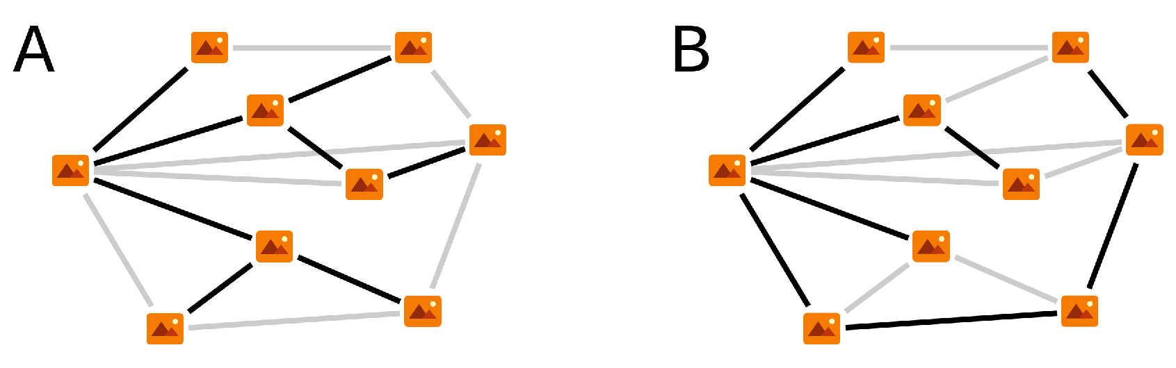
  In both cases, the ability of the pairs of pixels to align with the proposed transformation is validated using RANdom SAmple Consensus (RANSAC). The outcome of this feature matching process is a set of observed connections, each of them consisting of pairs of pixels that are consistent with the given transformation (whose coefficients are not kept), for some of the image-to-image pairs.
• Image clustering: Once a set of the observed connections among the images is available, the set of transformations for co-registration is obtained by a cluster analysis where we have the following:

  (I)

  The images are clustered taking into account the image-to-image observed connections and a required degree of connectivity;

  (II)

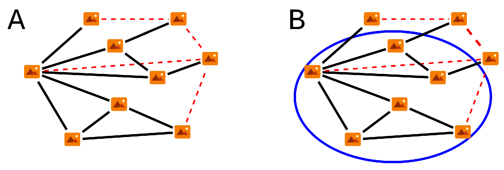
  For the largest cluster (or group), the set of transformations is obtained with a RANSAC approach that uses the image-to-image pairs from the feature pairing step.

  As a result of this second step, we obtain a subset of images and the transformations required to co-register them. It is considered that the (usually few) images that are not included in this subset of images cannot be co-registered.

The provided codes also include an initial step for downloading images and a final step that generates easily usable results. The codes are available at https://github.com/Ulises-ICM-UPC/UOrtos (accessed on 19 March 2025).

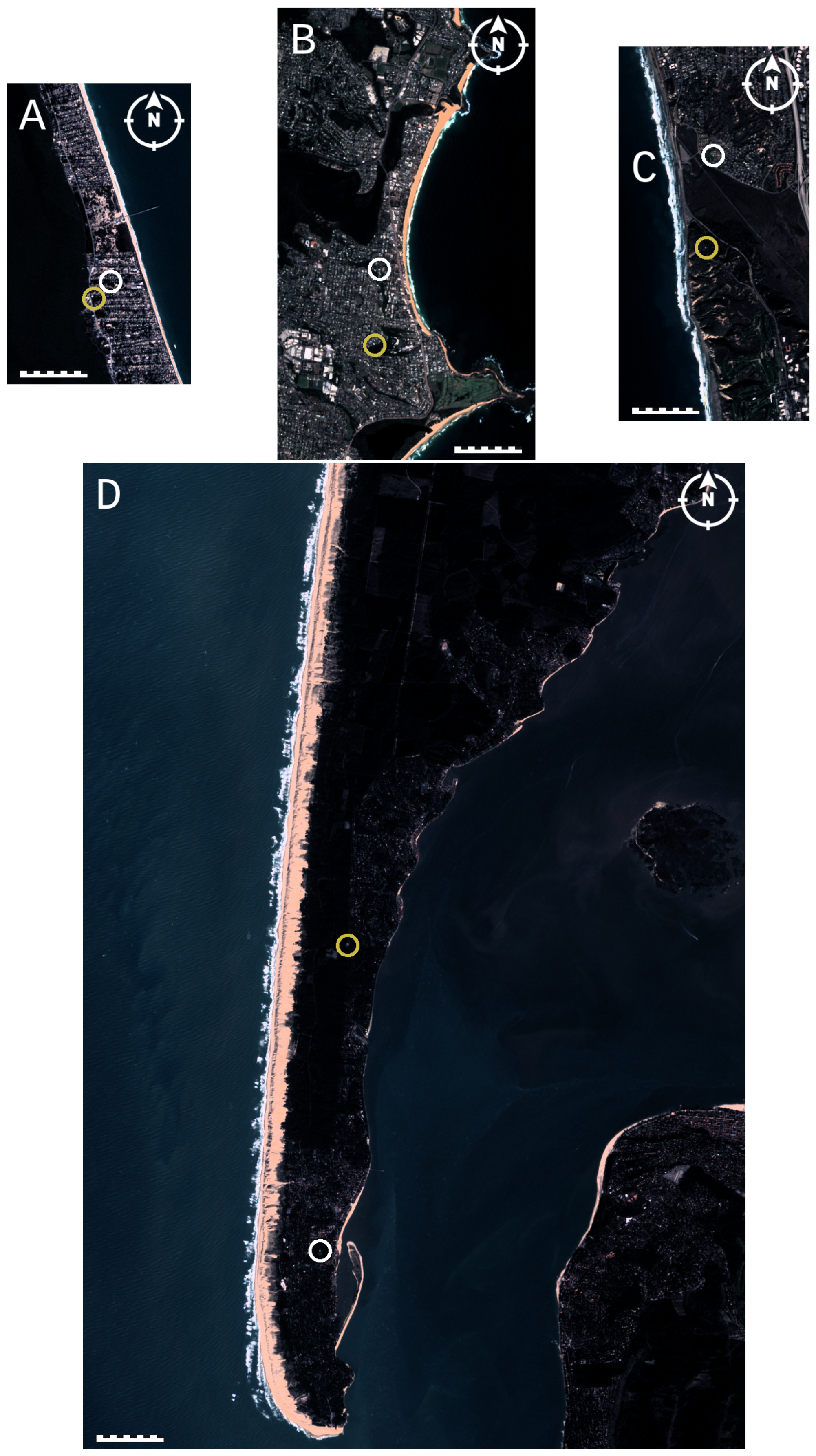
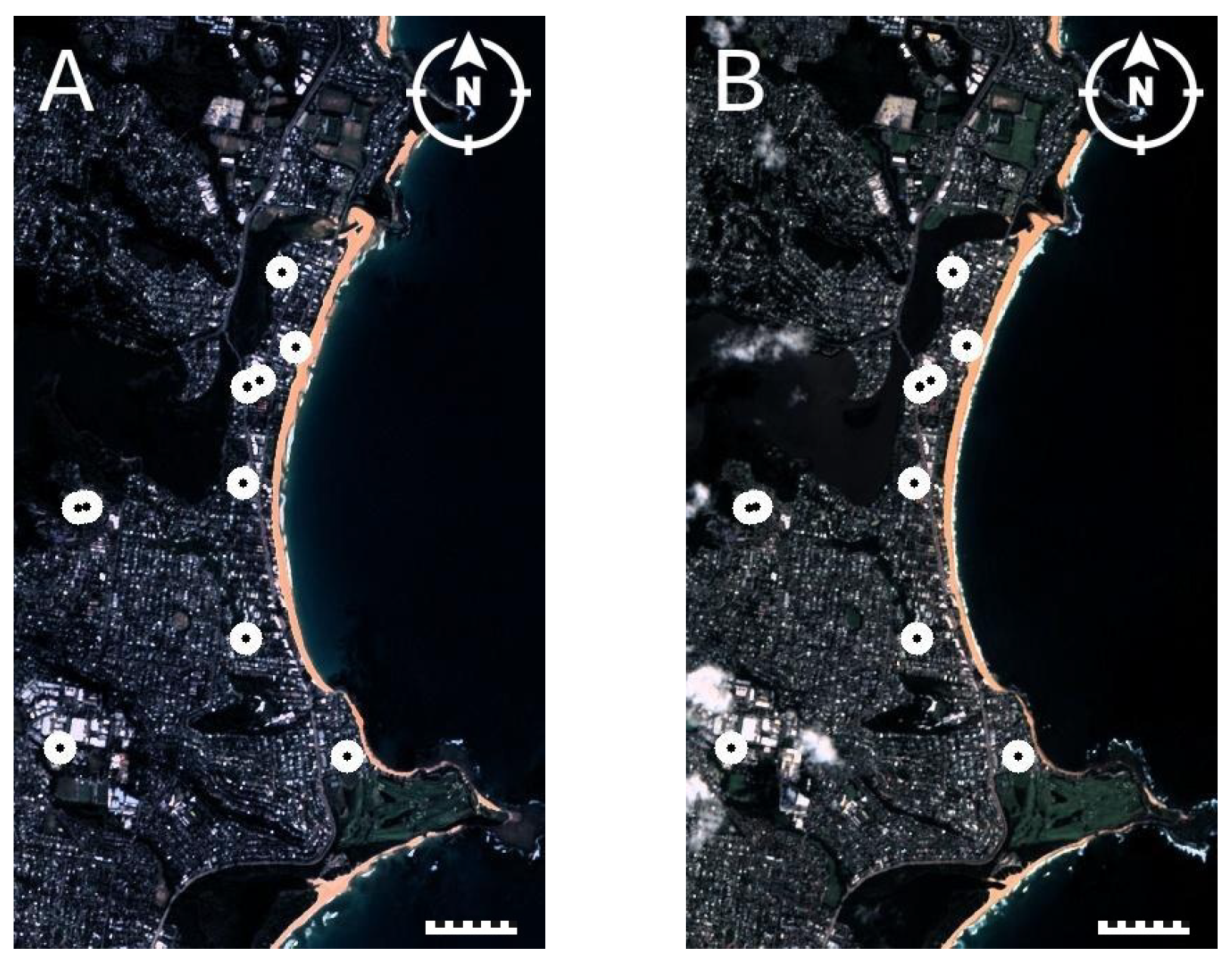
2.1. Study Sites

To test the proposed methodology we will, for convenience, use the same four locations as those in [2], namely, Duck, Narrabeen, Torrey Pines, and Truc Vert. The proposed domains encompass a range of conditions. Specifically, we compare the following: (1) urban areas (Duck, Narrabeen, Torrey Pines, plus Gandia) versus non-urban areas (Truc Vert); (2) regions with water on both sides (Duck and Truc Vert) versus those with water on only one side (the other); and (3) larger domains (Truc Vert) versus smaller ones (the others). Additionally, the location of Gandia will be included in the discussion, and only in the discussion, to highlight the effect of rotation in the transformation. The longitude and latitude of the central points of the Areas of Interest (AoIs), along with their respective widths and heights, are provided in

Table 1. Location (of the center) and size of the different AoIs considered. All coordinates are expressed in the WGS84 reference system, using latitude and longitude in decimal format.

Location	Lon [°]	Lat [°]	Width [km]	Height [km]
Duck	$-75.755$	$36.180$	$2.74$	$4.47$
Narrabeen	$151.300$	$-33.720$	$3.83$	$6.72$
Torrey Pines	$-117.255$	$32.925$	$2.82$	$3.34$
Truc Vert	$-1.230$	$44.685$	$9.84$	$14.65$
Gandia	$-0.160$	$38.995$	$3.59$	$3.46$

, while Figure 1 displays sample images.

We consider here 4 years (2020 to 2023, both included) of images from Sentinel-2 and Landsat programs for the four locations in Figure 1. We use two different sets of images for each AoI: images with a resolution of 10 m (only Sentinel-2) and images with a resolution of 30 m (Landsat and resampled Sentinel-2).

Table 2. Number of images (n) available for the different sites and resolutions considered.

	Resolution
Location	10-m	30-m
Duck	177	200
Narrabeen	142	163
Torrey Pines	219	259
Truc Vert	53	93
Gandia	201	275

shows the amount of images available in each case—the information of Gandia, only for the discussion, is also included.

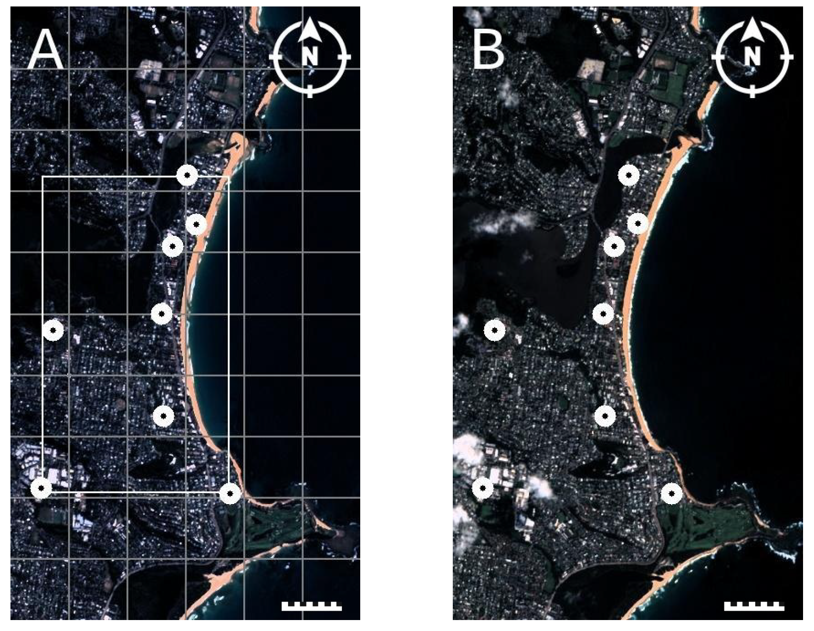
2.2. Feature Pairing

Given a set of n images, there are

$$N={\displaystyle \frac{n\left(n-1\right)}{2}},$$

(1)

pairs of different images.

2.2.1. Feature Pairing (I): Global ORB

For each of these N pairs, the two images are compared to identify feature pairs using the Oriented FAST and Rotated BRIEF (ORB) matching algorithm [23] or, alternatively, the Scale-Invariant Feature Transform (SIFT) matching algorithm [24]. The chosen algorithm is executed with a maximum user-defined number of features, $n_{\mathrm{FM}}$ (

Table 3. Overview of user-defined parameters introduced throughout the steps of the proposed methodology (as described in the text), along with their suggested default values. Here, “rot” stands for rotation, and can be set to “free” (${\alpha }_{ij}$ can be $\ne 0$) or “null” (${\alpha }_{ij}=0$, only translation).

Step	${\mathit{n}}_{\mathbf{FM}}$	rot	${\mathit{e}}_1$	${\mathit{n}}_{\mathbf{boxes}}$	${\mathit{n}}_{\mathbf{pairs}}$	f	${\mathit{e}}_2$	d	${\mathit{n}}_{\mathbf{sets}}$
feature pairing (I)	✓	✓	✓	✓	✓	✓	—	—	—
feature pairing (II)	—	✓	—	✓	✓	✓	✓	—	—
image clustering (I)	—	—	—	—	—	—	—	✓	—
image clustering (II)	—	✓	—	✓	✓	✓	✓	✓	✓
default values	1000	free	$1.0\mathrm{px}$	50	5	$0.5$	$0.2\mathrm{px}$	2	500

summarizes the user-defined parameters of the proposed methodology and provides reasonable default values), and small critical values of the allowed errors so as to reduce outliers. Figure 2 displays a set of matched pixel pairs for one image pair from Narrabeen.

Since we assume that we work with orthorectified images, the pixels, with coordinates $\left(c,r\right)$—for column c and row r—corresponding to the same feature as observed in two images (i and j) are related by the specific transformation relationship

$$\left(\begin{array}{c}{c}_j\\ r_j\end{array}\right)=\left(\begin{array}{cc}+cos{\alpha }_{ij}& +sin{\alpha }_{ij}\\ -sin{\alpha }_{ij}& +cos{\alpha }_{ij}\end{array}\right)·\left(\begin{array}{c}{c}_i\\ r_i\end{array}\right)+\left(\begin{array}{c}{d}_{c,ij}\\ d_{r,ij}\end{array}\right).$$

(2)

Equation (2) includes 3 parameters: rotation (${\alpha }_{ij}$) and translation ($d_{c,ij}$ and $d_{r,ij}$). Some works assume that there is no rotation (i.e., ${\alpha }_{ij}=0$) so that the above becomes a translation—this option is also available here. If the original images were perfectly co-registered, the transformation between any two images would be such that ${\alpha }_{ij}=d_{c,ij}=d_{r,ij}=0$. This happens not to be the case and, actually, the goal of this work is to obtain the coefficients $\left\{{\alpha }_{ij},d_{c,ij},d_{r,ij}\right\}$ for any two images i and j.

Note that the coefficients define the transformation from image “i” to image “j” but also the inverse. Also, note that the composition of any two transformations of the form in Equation (2) gives the same kind of transformation. In the following, to obtain the transformation (and an evaluation of its quality as discussed below) between two images, we consider for convenience that $1⩽i<j⩽n$: we assume that if the transformation of pixels from image i to image j is known and reliable, the inverse transformation is also known and trustworthy.

For two images i and j, given the set of K pairs of pixels provided by the feature matcher (ORB or SIFT), $\left(c_{i,k},r_{i,k}\right)$ and $\left(c_{j,k},r_{j,k}\right)$ for $k=1,\dots ,K$ (e.g., Figure 2, where $K=9$), all three values ${\alpha }_{ij}$, $d_{c,ij}$ and $d_{r,ij}$ can be obtained by minimizing the error

$$\sum _{k=1}^K{\left(c_{j,k}-{\widehat{c}}_{j,k}\right)}^2+{\left(r_{j,k}-{\widehat{r}}_{j,k}\right)}^2,$$

where $\left({\widehat{c}}_{j,k},{\widehat{r}}_{j,k}\right)$ are obtained applying Equation (2) to $\left(c_{i,k},r_{i,k}\right)$. This minimization process is highly optimized in the codes.

To eliminate all the incorrect pairs initially identified by the feature matcher, a purge is performed using RANdom SAmple Consensus (RANSAC) [19]. RANSAC is an iterative algorithm used to estimate a mathematical model (in our case the Equation (2) with 3 free parameters) from a dataset (the pairs) that contains outliers. It randomly selects a subset of data points (2 pairs in our case), fits the model to them, and evaluates the consensus by counting inliers, iterating until the best model with the highest consensus is found. The allowable error for the inliers in the RANSAC process, here $e_1$, is set to approximately $1.0\mathrm{px}$, but it is actually a user-defined parameter (Table 3). This value is considered to discard clearly erroneous pixel pairs; a more precise refinement of pixel pairs is carried out in subsequent steps. The RANSAC can be applied to obtain the model, but we use it mainly to eliminate outliers.

After performing the RANSAC analysis, only the best pairs (according to the errors provided by the feature matcher) are retained for each cell of a grid. This grid (thin gray lines in Figure 3A) is built so as to have a minimum of $n_{\mathrm{boxes}}$ cells ($n_{\mathrm{boxes}}$ being user-defined; see Table 3).

Two images i and j are considered a good FM-connection if both the number of pairs of pixels is $⩾n_{\mathrm{pairs}}$ ($n_{\mathrm{pairs}}$ being user-defined; see Table 3) and the box built using the limits of the pixels in image i (white box in Figure 3A) is such that its width is $⩾f{n}_c$ ($n_c$ is the number of columns of the image) and its height is $⩾f{n}_r$ ($n_r$ is the number of rows of the image), where f ($0<f<1$) is user defined (Table 3). This extra parameter f is introduced to further ensure that the pixels are well distributed along the image. Importantly, the number of good FM-connections obtained at this step is here named $m_1$, and is such that $m_1⩽N$.

Recapping, this step introduces the following user-defined parameters: $n_{\mathrm{FM}}$, $e_1$, $n_{\mathrm{boxes}}$, $n_{\mathrm{pairs}}$, and f. Additionally, the user has the option to set the coefficient as ${\alpha }_{ij}=0$ ($\mathrm{rot}=\mathrm{null}$) or leave it free ($\mathrm{rot}=\mathrm{free}$). Table 3 includes these and other parameters to follow, as well as reasonable (default) values. The influence of some of these parameters on the results of the various steps are analyzed in Section 3.

2.2.2. Feature Pairing (II): Local Correlation

For each pair of pixels of each of the $m_1$ good FM-connections above, an improvement of the feature localization is performed through a cross-correlation [25,26] performed locally. To optimize the cross-correlation process, for each of the $m_1$ pairs of connected images, one image is previously transformed into the other image domain using the parameters obtained with the pairs of initial feature pixels. This is particularly useful if the transformation between both images includes a significant rotation. Once the feature localization of the pairs has been improved, the same RANSAC purge procedure described in Section 2.2 is carried out now using a more restrictive (smaller) user-defined error, $e_2$ (which now can be $\ll e_1$), and the grid and f conditions are again required. In this way, we obtain the set of $m_2⩽m_1⩽N$ called observed connections. Notice that only the feature pair locations are kept, the transformation parameters being not necessary at this point.

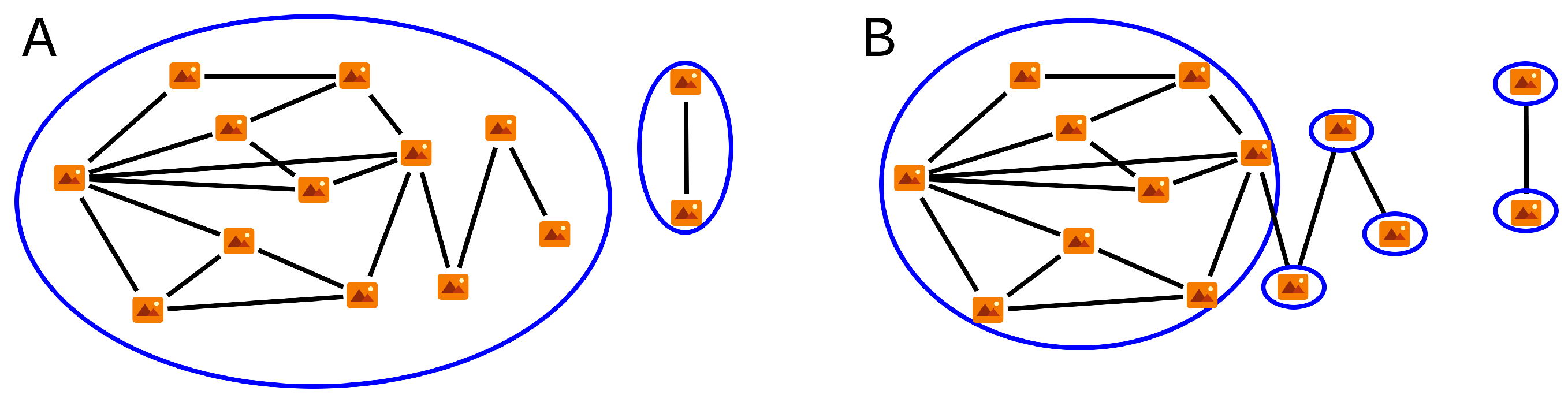
2.3. Image Clustering and Transformations

The set of $m_2$ observed connections obtained in the previous step is considered the ground truth for this stage. The goal here is to derive a highly robust set of transformations among the maximum number of images while systematically excluding those that cannot be reliably connected to the rest.

2.3.1. Image Clustering (I): Initial Clustering

A graph is first built where the images are the vertices, and the observed connections are the edges (see Figure 4 as an illustration with $n=14$ images and $m_2=19$ observed connections). From this graph, we form groups by ensuring that each image in a group is directly connected to at least d (degree) other images of the same group (d being a user-defined parameter; see Table 3). Figure 5 illustrates the groups, with ovals, derived from the graph in Figure 4 using $d=1$ and $d=2$ (A and B respectively). Not surprisingly, as the degree d increases, the number of groups generally increases. While setting $d=1$ is sufficient to obtain all transformations for the images within a group, increasing to $d=2$ ensures that all images belong to some cycle (which does not happen with $d=1$; see the images at the right of the largest group in Figure 5A). This enables the double-checking of transformations, which avoids error propagation and enhances quality.

The size of the largest group obtained in this step is called $s_1$. It is of interest for $s_1$ to be as large as possible (close to n) so that the maximum number of images can be co-registered. In Figure 6, $s_1=12$ if $d=1$ and $s_1=9$ if $d=2$.

2.3.2. Image Clustering (II): Transformations, RANSAC Analysis and Final Clustering

For each of the groups obtained in the initial clustering, a unique set of transformations is determined, consisting of terns $\left({\alpha }_{ij},d_{c,ij},d_{r,ij}\right)$, which enable the transformation of pixel coordinates between any pair of images i and j within the group. Actually, our main interest is in the largest group, containing the great majority of the images.

Adopting the RANSAC approach, we generate multiple random sets of transformations and then select the one that provides the best results. To randomly derive one set of transformations, we consider a two-step procedure (here for the largest group of size $s_1$):

• First, we obtain a random walk with $s_1-1$ edges connecting all the images through the observed connections, such as the 2 examples of random walks shown in Figure 6 for the largest group in Figure 5B;
• Then, for a given random walk, we obtain the corresponding $s_1-1$ transformations by choosing, for each edge (observed connection), $n_{\mathrm{pairs}}$ random pairs of pixels (recall that there are at least $n_{\mathrm{pairs}}$ pairs of feature pixels for each connection); the set of $s_1-1$ transformations allows to relate any two images of the group.

The quality of every set of transformations is assessed in the following way. Given one pair of images (i and j) out of the $m_2$ observed connections, we consider that this connection is recovered by the set of transformations if, when sending the pixels of i to j via the transformation proposed by this set, the number of pixels with errors below $e_2$ is $⩾n_{\mathrm{pairs}}$ and they are well distributed (in the same way as in Section 2.2, i.e., applying the grid and f conditions). Figure 7A illustrates how, for the random walk in Figure 6A, some connections can be recovered (black lines) while others not (dashed red lines). The quality of a set of transformations is assessed by the number of recovered connections.

Following the RANSAC philosophy, a large number of random walks is proposed, and the final set of transformations is considered to be the one maximizing the number of recovered connections. The amount of sets considered in the analysis is given by a user-defined parameter ($n_{\mathrm{sets}}$, Table 3). Once the best set of transformations and the recovered connections are reached, the images are again clustered as in the previous step—“Image clustering (I)” (see Figure 7B). The size of the largest obtained group is $s_2$.

When using UOrtos, the user is given the possibility to include a georeferenced image to the rest of images that are automatically downloaded from GEE when running UOrtos. If that is the case and, further, the provided image is part of the $s_2$ co-registered images, it is considered the reference image, and the transformations are referred to it. Otherwise, once the largest group of co-registrable images and the corresponding transformations are obtained, the reference image is considered to be the most centered image in the group, i.e., the image minimizing a global distance relative to the remainder images of the group. For this purpose, given two images i and j of $n_c\times n_r$ pixels, and given a transformation $\left\{{\alpha }_{ij},d_{c,ij},d_{r,ij}\right\}$, we define

$$d_{ij}^2={\displaystyle \frac{1}{n_c{n}_r}}\sum _{c=1}^{n_c}\sum _{r=1}^{n_r}\left[{\left(c-\widehat{c}\right)}^2+{\left(r-\widehat{r}\right)}^2\right],$$

(3)

where, recalling expression (2)

$$\begin{array}{cc}\hfill \widehat{c}& =+ccos{\alpha }_{ij}+rsin{\alpha }_{ij}+d_{c,ij},\hfill \\ \hfill \widehat{r}& =-csin{\alpha }_{ij}+rcos{\alpha }_{ij}+d_{r,ij}.\hfill \end{array}$$

The above expression (3) gives a measure of the (squared) size of the transformation from i to j. The reference image is the one that minimizes

$$d_i^2=\sum _j{d}_{ij}^2,$$

where j runs in all images of the group.

3. Results

Both ORB and SIFT can be used as feature matching algorithms as described in the methodology. The user can choose between the two by simply setting the value of a variable in the parameters file. For convenience, the following results and discussion focus on the use of ORB, as it provides insights into the influence of other parameters in the same way that SIFT does. In fact, preliminary tests indicate that SIFT tends to yield a higher number of feature pairs and slightly higher $s_2$ values, albeit at a greater computational cost.

3.1. Feature Pairing

The first step of the feature pairing, global feature matching, allows to obtain a set of ($m_1$) good FM-connections, and introduces the following parameters (Table 3): $n_{\mathrm{FM}}$, rot, $e_1$, $n_{\mathrm{boxes}}$, $n_{\mathrm{pairs}}$ and f. Regarding $n_{\mathrm{FM}}$, the number of features obtained, a value of 1000 has been shown to work well in all sites. Increasing this value to 2000 roughly quadruples the computational time of this step without having a noticeable impact on $m_1$, while reducing it to 500 has a significant negative impact on $m_1$. The rotation (rot) is set to be free as the default to allow for the transformation to absorb potential rotations. As previously mentioned, the error $e_1$ is set to 1 px. The recommended value of $n_{\mathrm{boxes}}=50$ (Table 3) is sufficiently large so as to allow the points to be well distributed across the entire image. The default value $n_{\mathrm{pairs}}=5$ is chosen based on the fact that at least 2 pairs are necessary to obtain the parameters of the transformation between two images; doubling this number (in fact, multiplying it by 2.5) helps to avoid issues related with over-parametrization.

Finally, the parameter f is to be selected based on the specific characteristics of each site, as some locations may contain large featureless areas, such as the sea, something particularly evident in Duck (Figure 1A). Figure 8 illustrates the effect of f on $m_1/N(⩽$1), where N represents the total number of possible image pairs (see Equation (1)). All other parameters are set to their previously described default values. Decreasing f, i.e., making the criteria less restrictive, increases the number of connections $m_1$. However, reducing it too much could compromise the overall quality of the co-registration due to diminished coverage. A well-balanced value of f is essential for optimal performance of the proposed methodology. While users can explore the best value depending on the specific AoI, we will hereafter consider $f=0.5$ as the default in all cases. This value provides substantial image coverage and allows us to evaluate the impact of $m_1/N$ on the final results (for $f=0.5$, $m_1/N$ is significantly smaller for Duck as shown in Figure 8).

The second feature pairing step, local correlation, introduces the more restrictive error $e_2$ (Table 3). The impact of this error on the number of the final observed connections, $m_2$, is shown in Figure 9 for the default values of the other parameters in Table 3. Note that, as expected, as $e_2$ increases and becomes less restrictive, its influence on $m_2$ diminishes, and $m_2$ approaches $m_1$ (i.e., the values shown in Figure 8 for $f=0.5$).

3.2. Image Clustering and Transformations

The image clustering process introduces the degree of connection, d. The sizes of the largest group obtained after the RANSAC-like process using random walks $s_2$ are shown in Figure 10 for the four locations as a function of $e_2$ and d.

It can be observed that the influence of $e_2$ on $s_2$ decreases as $e_2$ increases, becoming nearly negligible for $e_2\gtrsim 0.4$. Additionally, the values of $s_2$ are smaller for $d=2$ (solid lines) compared to $d=1$ (dash-dotted), particularly when both values are significantly smaller than 1. The $s_2$ values are generally higher for images with a 10 m resolution (Figure 10A) than for those with a 30 m resolution (Figure 10B). Except for Duck beach—where $m_2$ is notably small—the ratio $s_2/n$ exceeds $0.9$ (90% of images co-registered) for $e_2⩾0.2$ for 10 m resolution images and is nearly the same for 30 m resolution images. For instance, in the case of Narrabeen beach, with $e_2=0.2$ and $d=2$, $s_2=140$ out of $n=142$ images; only 2 images cannot be co-registered. Figure 11 shows, for this specific case, the reference image, one of the two non co-registered images due to cloud cover, and a third image that, despite the partial presence of clouds, is successfully co-registered.

The random walk RANSAC-like proposed process provides, together with the largest group, the transformations of all the images to the reference image. For illustration purposes mainly, the values of the $\alpha$, $d_c$ and $d_r$ corresponding to the obtained transformations are shown in Figure 12 for 10 m resolution images of Duck and Narrabeen. The reference image is highlighted in both cases with a vertical dotted line, and the images that are not included in the largest group, i.e., the images that are not co-registered, are denoted with red dots. According to Figure 10A, these images represent around $30\%$ and $1.5\%$ of the total images of Duck and Narrabeen, respectively. As can be seen in Figure 12, the rotation angles are smaller than $0.1^{\circ }$, and $d_c$ and $d_r$ are generally smaller than 1 px. This also occurs in the other two sites for the 10 m resolution images. For the 30 m resolution images, the angles are up to $0.2^{\circ }$ and the displacements $d_c$ and $d_r$ up to $0.4$ px.

The significance of the transformations in terms of pixel shifts is illustrated in Figure 13 (for the two cases shown in Figure 12). Figure 13 depicts how the positions of specific pixels (points 1 and 2 in the left panels) change when the transformations are applied. In the plots on the right panels, the red dot represents the selected pixel in the reference image, while the black dots display the results of applying the transformations from the reference image to the remaining $s_2-1$ images of the group. In other words, the black dots represent the estimated pixel coordinates of the same feature across the different images.

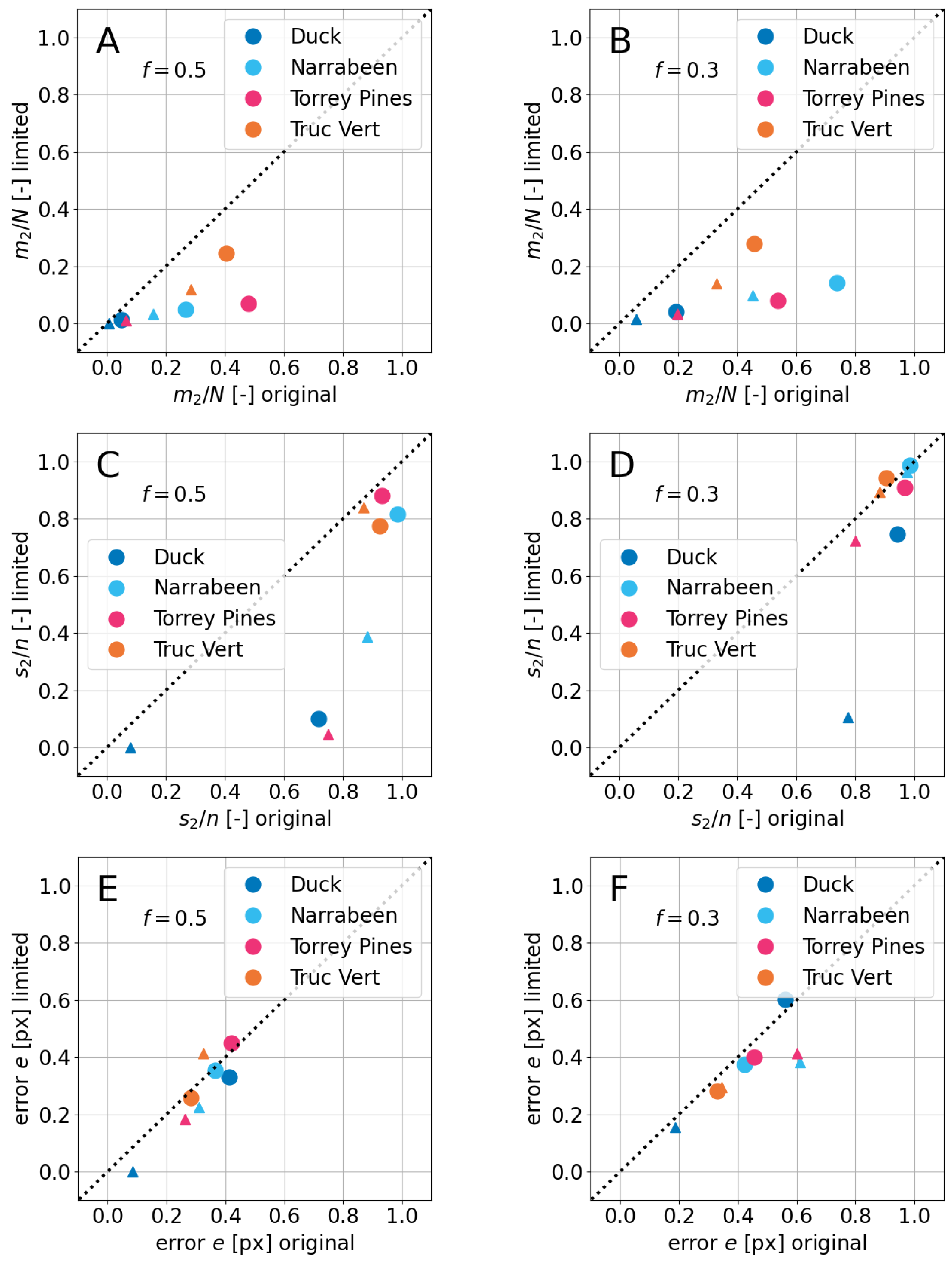
3.3. Validation

The right panels in Figure 13 show that the expected displacement of the same feature across different images is up to a few pixels. However, a proper evaluation of the quality of the obtained transformations is still missing. To address this, a clearly identifiable feature for each AoI and resolution is manually tracked across all available images. These features are circled in Figure 1 for all four AoIs and both resolutions, and in Figure 13 for Duck and Narrabeen at 10 m resolution (the same cases illustrated in Figure 12 and Figure 13). For these two latter cases, these features are shown in closer detail in the left panels of Figure 14. It should be noted that the manual tracking of these features is subject to error.

The right panels of Figure 14 show the tracked pixel coordinates for the same feature across all the original images in black and, in red, these coordinates after being transformed to the reference image using the transformations from Figure 12. Note that the plots in Figure 14 resemble those in Figure 13 but now with a cloud of red points instead of a single red dot. These plots are equivalent; the red clouds would reduce to a single point if both the manual tracking and the transformations were flawless.

Given a cloud of points, we define its size (what is to be the error) as the maximum distance of any point to the center of gravity of the cloud. We furthermore define the error e associated to a set of transformations as the size of the red cloud in Figure 14, obtained from the manually tracked positions of the circled feature and the transformations. We consider the maximum distance rather than the Root Mean Squared Error, for we are focused on avoiding outlier images (i.e., wrongly co-registered images) to ensure the robustness and accuracy of the subsequent performed analyses. Figure 15 shows the evolution of the error e as a function of $e_2$ and d for all the sites and both resolutions.

For $d=2$—i.e., solid lines in Figure 15—the errors e remain consistently below $\sim 0.4$ when $e_2⩽0.2$. As $e_2$ increases, the error e generally rises to values up to $0.6$ for $d=2$. In contrast, for $d=1$, the errors can reach higher values and, more importantly, they do not decrease when $e_2⩽0.2$, particularly for the 10 m resolution images (Figure 15A). For $d=2$ and $e_2=0.2$ and the other default values for the rest of parameters,

Table 4. Error e [px] before (left columns) and after (right columns) the co-registration, obtained using the default parameter values in Table 3.

	Pre Co-Register		Post Co-Register
Location	10-m	30-m	10-m	30-m
Duck	$1.872$	$0.072$	$0.414$	$0.083$
Narrabeen	$1.078$	$0.127$	$0.365$	$0.310$
Torrey Pines	$1.347$	$0.150$	$0.420$	$0.263$
Truc Vert	$1.106$	$0.688$	$0.281$	$0.324$

shows the error prior to and after the co-registration for all sites (e.g., the sizes of the black and red clouds shown in Figure 14, respectively). In the 10 m resolution images, there is a clear decrease from more than 1 px to $0.4$ px or less. Errors below $0.4$ px are considered indiscernible, as the estimated error in manual tracking is of the same order, meaning that the actual error may be smaller than $0.4$ px. In the 30 m resolution images, the errors before co-registration are already below $0.4$ px in most sites, and thereby no error decrease is obtained. Only in the Truc Vert case, with the largest image size, the original error is of $0.7$ px and it decreases to $0.3$ px.

4. Discussion

An analysis of Figure 10 ($s_2$, number of co-registered images) and Figure 15 (co-registration errors e) indicates that the combination of $e_2=0.2$ and $d=2$ generally provides values of $s_2$ close to n, while keeping the error e below $0.4$—recall that $e⩽0.4$ can be considered indiscernible due to the errors in the manual tracking. This guarantees that a large amount of the original images can be kept while ensuring that co-registration errors are minor. In most of the 30 m resolution images, the original errors are already below $0.4$ px (Table 4) but, even in these cases, applying this methodology can still be useful since it ensures that the final obtained image set does not contain outliers.

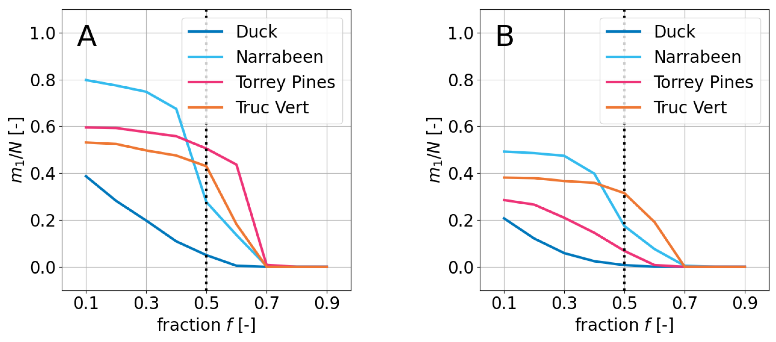
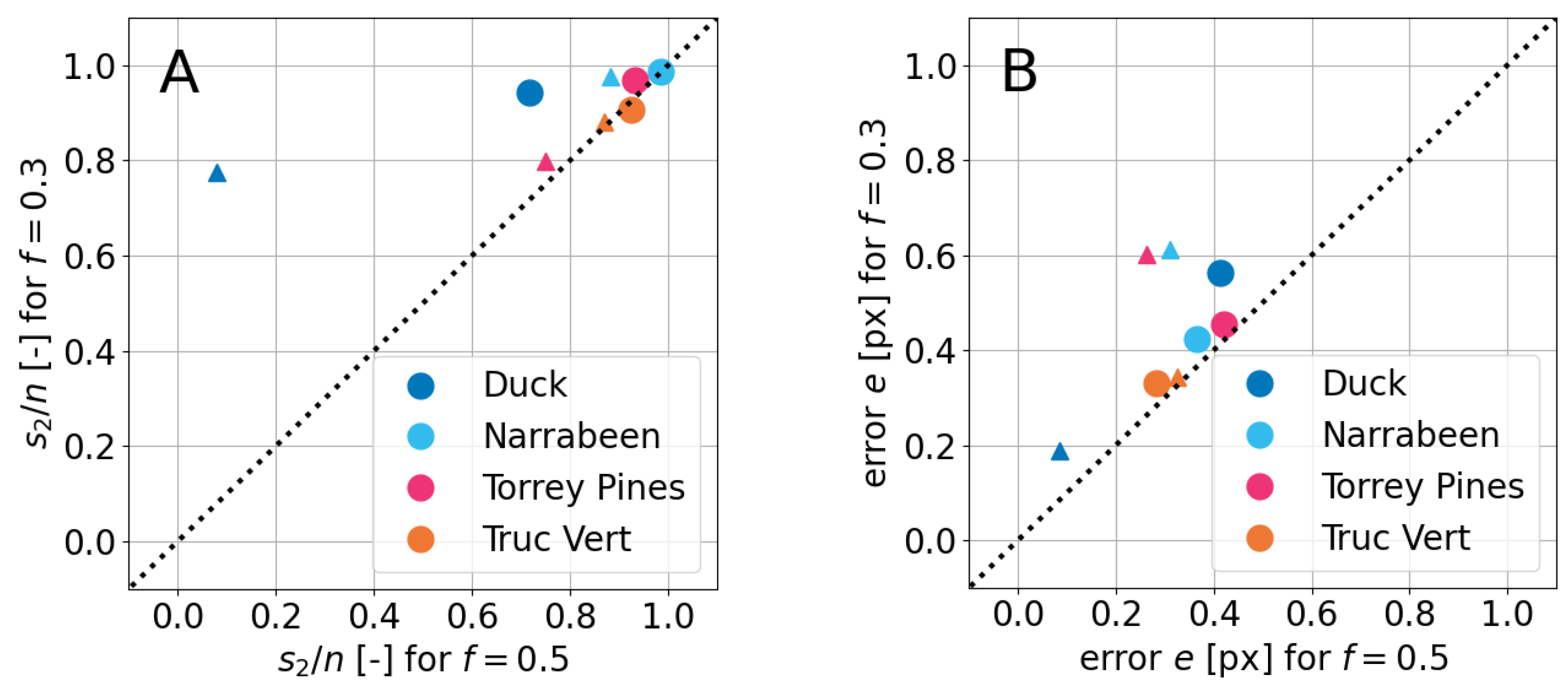
4.1. On the Influence of f

The low values of $s_2$ for Duck stand out in Figure 10, especially for the 30 m resolution images. This result could likely have been anticipated from Figure 8 and Figure 9, which showed a very small number of observed connections. A closer look at Figure 8, which illustrates the influence of f on $m_1$ (and subsequently on $m_2$ and $s_2$), suggests that being less restrictive with the value of f—i.e., decreasing it—for Duck images could potentially increase the number of co-registered images.

Figure 16A shows the change in the values of $s_2/n$ when f is reduced from $0.5$ to $0.3$. In general, the values of $s_2$ increase. It is important to note that the methodology involves random processes, so results can occasionally decrease, although for the default values, the observed differences from different realizations are always below $2\%$ in $s_2$. The improvement is particularly noticeable for Duck at 30 m resolution.

The impact of reducing f from $0.5$ to $0.3$ on the error e is shown in Figure 16B. The errors increase to values up to $0.6$. Although for Duck at 30 m resolution—the case that motivated this analysis—the error e remains small, it should be noted that the error, which will generally be unknown, could reach higher values in other realizations. For a given AoI, we recommend that users initially set f to the highest reasonable possible value, and then verify that the number of co-registered images is satisfactory. If an overly high f results in a significant drop—likely due to the distribution of featureless areas—a reduction in f should be considered.

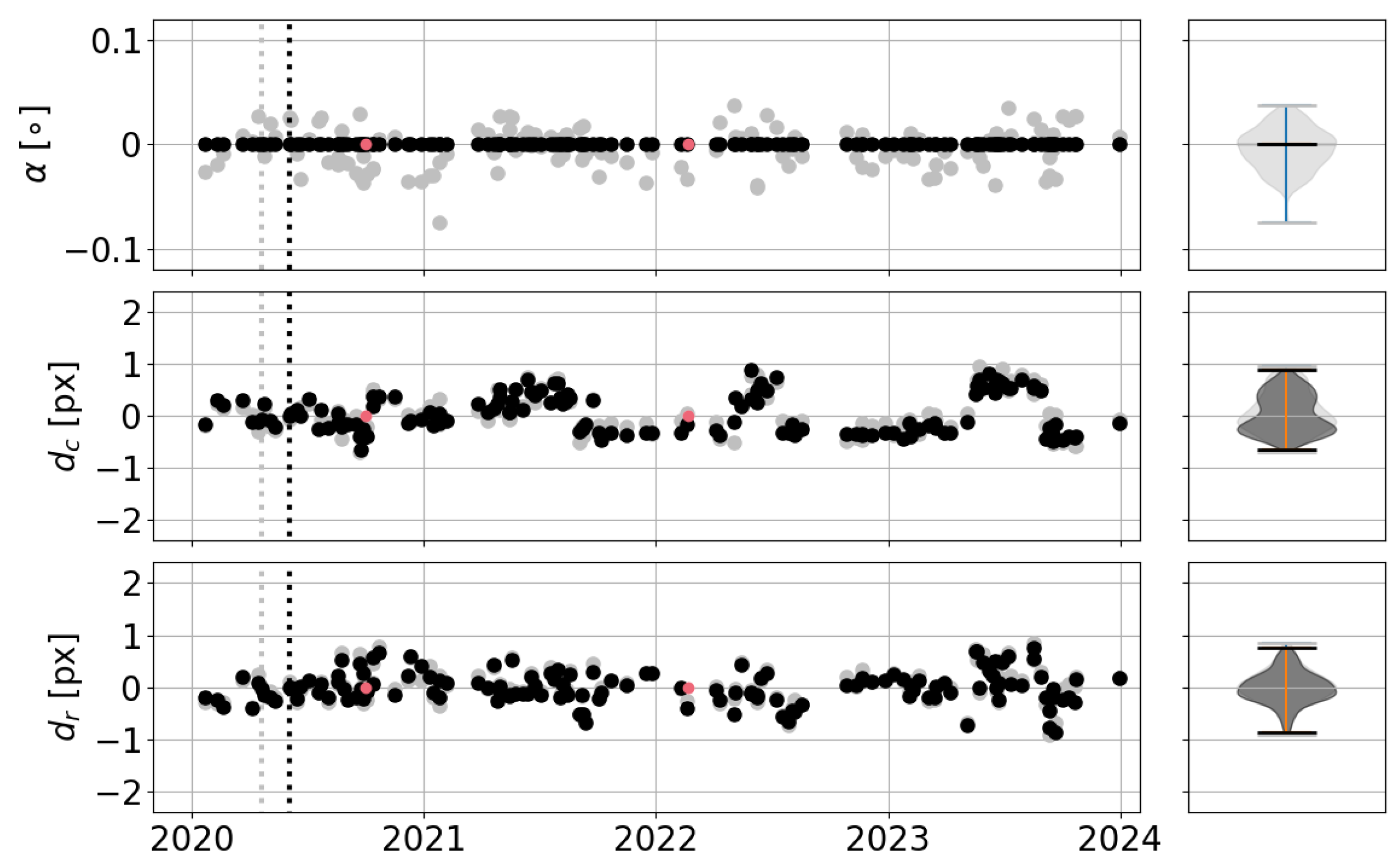
4.2. Null Rotation Case

Rotation is often disregarded in image co-registration. The presented algorithm allows for this by setting “rot” to “null” (as opposed to “free” as shown in Table 3). In the four cases analyzed here, the differences in the transformations between both options happen to be minimal. Figure 17 illustrates these differences—regarding the transformation to their respective reference image—when using “null” (bolder colors) versus “free” (lighter colors) for Narrabeen beach at 10 m resolution. Given the small values of $\alpha$ in the “free” case, with $\left|\alpha \right|\lesssim 0.{05}^{\circ }$ (that represents a movement of around $0.3$ pixels at the corners for Narrabeen beach), it is unsurprising that the differences in $d_c$ and $d_r$ behavior are minor. In fact, the errors e are also very similar for all four locations and for both resolutions, whether “free” or “null” is used (below $0.01$ pixels in all tested cases).

However, to test the feasibility of this methodology to automatically handle images with a relative rotation, we study the case of Gandia beach (Table 1 and Table 2). Since this portion of the coast is located in the intersection of two different UTM zones (30 and 31), the images automatically downloaded by GEE can be in two different projections. As a result of this, some images could appear significantly rotated relative to the others (Figure 18).

To avoid this problem, images of one projection only are typically downloaded and this is also an option in the present methodology. Alternatively, by allowing the rotation to be free, the proposed algorithm could also handle this situation by determining the necessary rotation angles. In any case, this property of Gandia beach allows us to illustrate how the proposed methodology works when a relative rotation between images exist. Figure 19 displays the resulting transformations, showing a bimodal behavior in the rotation angle (notice that the histogram on the right unrealistically smooths out this behavior).

4.3. Very Large Datasets

From Equation (1), the maximum number of connections between images increases with the square of the dataset size ($N\sim n^2/2$). This squared growth can result in an unmanageable computational cost, as many subsequent operations must process the large number of generated connections. However, as the number of images increases, the ratio $s_2/n$ is more likely to improve since the probability of finding transition images that can connect the initially disconnected ones also increases.

To address the challenge of reducing the computational cost, the code provides an option to limit the number of observed connections for each image to a maximum value of “$\mathrm{limFM}$”. The selection of potential connections for each image is performed randomly, with a feature that prioritizes images with lower connection capacity (due to factors like cloud cover or lighting conditions), giving them a higher likelihood of reaching the maximum number of connections. By limiting the observed connections, the total number of connections is limited to $\mathrm{limFM}\times n$, i.e., a linear function of the number of images rather than a quadratic one.

Figure 20 presents a comparison between the original results (on the horizontal axis) and those obtained with $\mathrm{limFM}=25$ (on the vertical axis) for $f=0.5$ (Figure 20A,C,E) and $f=0.3$ (Figure 20B,D,F). We note that the algorithm was tested on an HP EliteBook 650 equipped with a 13th Gen Intel Core i5-1350P (12 cores/16 threads, up to 4700 MHz) and 32 GiB DDR4 RAM (3200 MHz). For the Torrey Pines dataset—the most computationally demanding, due to the number of images—the processing time was reduced from approximately 43 min (without limitation, with 65% of that time spent in the correlation step) to about 8 min when using limFM = 25. Moreover, since introducing limFM changes the computational cost from quadratic to linear growth with the number of images, the benefits will be even more pronounced for larger datasets.

The first consequence of limiting the number of connections is a significant reduction in the number of observed connections (ratio $m_2/N$, top panels in Figure 20), especially when $n\gg \mathrm{limFM}$, which is the case for all the studied beaches except Truc Vert for 10 m resolution (see Table 2). Despite this reduction, Figure 20C shows that for $f=0.5$, the size $s_2$ of the largest groups of co-registered images remain similar to the original except for Duck beach, which already shows problems related to f, and for Narrabeen and Torrey Pines at 30 m resolution. The relative performance improves when f is relaxed to $0.3$ (Figure 20D). In this case, except for Duck beach with 30 m resolution, the values of $s_2/n$ remain very similar with or without limiting the number of connections. This is particularly noteworthy because, as shown in the bottom panels, the error e remains essentially unaffected by the reduction in connections. It is important to note that, apart from f, the default parameter values in Table 2 are used throughout this analysis, including $e_2=0.2$ and $d=2$.

5. Conclusions

The results of this study suggest that the proposed co-registration methodology can improve the alignment of satellite images for shoreline detection and coastal monitoring. By addressing key challenges such as georeferencing errors and image rotation, the approach provides a useful framework for analyzing coastal dynamics across various environments. The main conclusions drawn from this work are as follows:

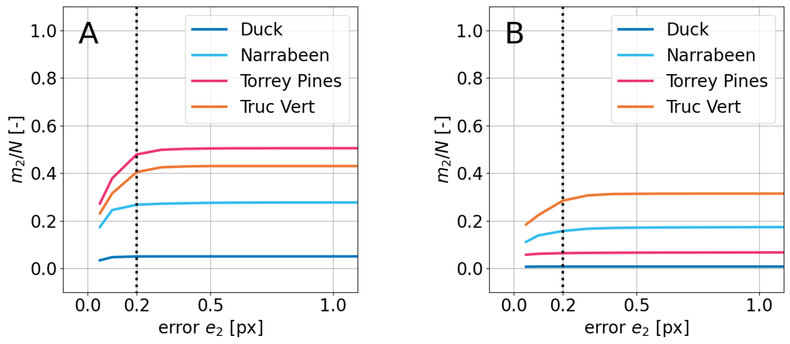
• Improved Image Alignment: The co-registration method, based on ORB/SIFT, local cross-correlation, and RANSAC, enhances the alignment of satellite images, potentially reducing the impact of georeferencing errors from 1 to at least 0.4 px (it is probably smaller, of the order of 0.2 px), in the tested 2020–2023 images of four sites. This could have a significant benefit on shoreline detection by reducing the present-day errors of 0.5–1 px, and enhance coastal monitoring.
• Outlier Reduction: The RANSAC-based filtering process seems to help in eliminating erroneous pixel-pair connections as well as bad image transformations, which contributes to more reliable transformations across the majority of the image set.
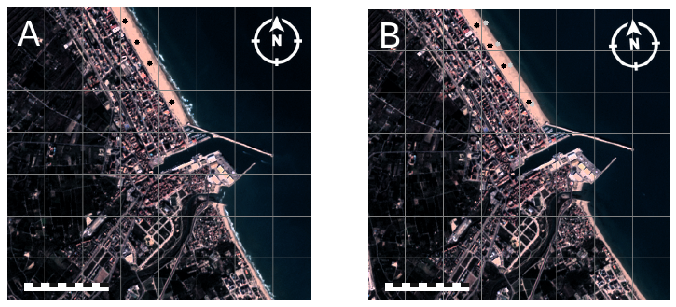
• Rotation Handling: The ability to account for image rotation, especially in cases involving different projections (e.g., Gandia), underscores the method’s flexibility. This suggests that the approach may work well even under challenging conditions.
• Flexibility and Applicability: The approach can be applied to different coastal environments and image resolutions as demonstrated by the present examples across multiple locations. Moreover, it remains adaptable to various datasets with minimal user input.
• Potential Applications: While further validation is needed, the method holds potential for applications in coastal management, disaster preparedness, and studying climate change impacts, particularly for monitoring short-term events such as storms and long-term shoreline evolution.
• Future Improvements: The method could benefit from future advancements in feature matching algorithms to further enhance its accuracy and efficiency. There is also room for future improvements, including optimizing the algorithm for very large datasets and integrating additional environmental data. The open-source nature of the tool could allow for further development and broader applications within the remote sensing community.

References

- Mentaschi, L.; Vousdoukas, M.; Pekel, J.F.; Voukouvalas, E.; Feyen, L. Global long-term observations of coastal erosion and accretion. Sci. Rep. 2018, 8, 12876. [Google Scholar] [CrossRef]
- Vos, K.; Splinter, K.; Palomar-Vázquez, J.; Pardo-Pascual, J.; Almonacid-Caballer, J.; Cabezas-Rabadán, C.; Kras, E.; Luijendijk, A.; Calkoen, F.; Almeida, L.; et al. Benchmarking satellite-derived shoreline mapping algorithms. Commun. Earth Environ. 2023, 4, 345. [Google Scholar] [CrossRef]
- Toure, S.; Diop, O.; Kpalma, K.; Maiga, A. Shoreline detection using optical remote sensing: A review. ISPRS Int. J. Geo-Inf. 2019, 8, 75. [Google Scholar] [CrossRef]
- Zulkifle, F.; Hassan, R.; Kasim, S.; Othman, R. A review on shoreline detection framework using remote sensing satellite image. Int. J. Innov. Comput. 2017, 7, 40–51. [Google Scholar]
- European Space Agency. Copernicus Programme—European Space Agency. 2024. Available online: https://www.copernicus.eu/en (accessed on 3 March 2025).
- Gorelick, N.; Hancher, M.; Dixon, M.; Ilyushchenko, S.; Thau, D.; Moore, R. Google Earth Engine: Planetary-scale geospatial analysis for everyone. Remote Sens. Environ. 2017, 202, 18–27. [Google Scholar] [CrossRef]
- Vos, K.; Splinter, K.; Harley, M.; Simmons, J.; Turner, I. CoastSat: A Google Earth Engine-enabled Python toolkit to extract shorelines from publicly available satellite imagery. Environ. Model. Softw. 2019, 122, 104528. [Google Scholar] [CrossRef]
- Sánchez-García, E.; Palomar-Vázquez, J.; Pardo-Pascual, J.; Almonacid-Caballer, J.; Cabezas-Rabadán, C.; Gómez-Pujol, L. An efficient protocol for accurate and massive shoreline definition from mid-resolution satellite imagery. Coast. Eng. 2020, 160, 103732. [Google Scholar] [CrossRef]
- Almeida, L.P.; Efraim de Oliveira, I.; Lyra, R.; Scaranto Dazzi, R.L.; Martins, V.G.; Henrique da Fontoura Klein, A. Coastal Analyst System from Space Imagery Engine (CASSIE): Shoreline management module. Environ. Model. Softw. 2021, 140, 105033. [Google Scholar] [CrossRef]
- Pardo-Pascual, J.; Almonacid-Caballer, J.; Cabezas-Rabadán, C.; Fernández-Sarría, A.; Armaroli, C.; Ciavola, P.; Montes, J.; Souto-Ceccon, P.; Palomar-Vázquez, J. Assessment of satellite-derived shorelines automatically extracted from Sentinel-2 imagery using SAET. Coast. Eng. 2024, 188, 104426. [Google Scholar] [CrossRef]
- Luijendijk, A.; Hagenaars, G.; Ranasinghe, R.; Baart, F.; Donchyts, G.; Aarninkhof, S. The State of the World’s Beaches. Sci. Rep. 2018, 8, 6641. [Google Scholar] [CrossRef]
- Mao, Y.; Harris, D.; Xie, Z.; Phinn, S. Efficient measurement of large-scale decadal shoreline change with increased accuracy in tide-dominated coastal environments with Google Earth Engine. ISPRS J. Photogramm. Remote Sens. 2021, 181, 385–399. [Google Scholar] [CrossRef]
- Enache, S.; Clerc, S.; Poustomis, F. Optical MPC Data Quality Report—Sentinel-2 L1C MSI. 2024. Available online: https://sentinels.copernicus.eu/documents/247904/4893455/OMPC.CS.APR.001+-+i1r0+-+S2+MSI+Annual+Performance+Report+2022.pdf (accessed on 19 March 2025).
- Gomes da Silva, P.; Jara, M.S.; Medina, R.; Beck, A.L.; Taji, M.A. On the use of satellite information to detect coastal change: Demonstration case on the coast of Spain. Coast. Eng. 2024, 191, 104517. [Google Scholar] [CrossRef]
- Rengarajan, R.; Choate, M.; Hasan, M.N.; Denevan, A. Co-registration accuracy between Landsat-8 and Sentinel-2 orthorectified products. Remote Sens. Environ. 2024, 301, 113947. [Google Scholar] [CrossRef]
- Brown, L.G. A survey of image registration techniques. ACM Comput. Surv. 1992, 24, 325–376. [Google Scholar] [CrossRef]
- Scheffler, D.; Hollstein, A.; Diedrich, H.; Segl, K.; Hostert, P. AROSICS: An automated and robust open-source image co-registration software for multi-sensor satellite data. Remote Sens. 2017, 9, 676. [Google Scholar] [CrossRef]
- Wong, A.; Clausi, D.A. ARRSI: Automatic Registration of Remote-Sensing Images. IEEE Trans. Geosci. Remote Sens. 2007, 45, 1483–1493. [Google Scholar] [CrossRef]
- Fischler, M.; Bolles, R. Random sample consensus: A Paradigm for Model Fitting with Applications to Image Analysis and Automated Cartography. Commun. ACM 1981, 24, 381–395. [Google Scholar] [CrossRef]
- Gao, F.; Masek, J.; Wolfe, R. Automated registration and orthorectification package for Landsat and Landsat-like data processing. J. Appl. Remote Sens. 2009, 3, 033515. [Google Scholar] [CrossRef]
- Behling, R.; Roessner, S.; Segl, K.; Kleinschmit, B.; Kaufmann, H. Robust automated image co-registration of optical multi-sensor time series data: Database generation for multi-temporal landslide detection. Remote Sens. 2014, 6, 2572–2600. [Google Scholar] [CrossRef]
- Yan, L.; Roy, D.; Zhang, H.; Li, J.; Huang, H. An automated approach for sub-pixel registration of Landsat-8 Operational Land Imager (OLI) and Sentinel-2 Multi Spectral Instrument (MSI) imagery. Remote Sens. 2016, 8, 520. [Google Scholar] [CrossRef]
- Rublee, E.; Rabaud, V.; Konolige, K.; Bradski, G. ORB: An efficient alternative to SIFT or SURF. In Proceedings of the 2011 International Conference on Computer Vision, Barcelona, Spain, 6–13 November 2011; pp. 2564–2571. [Google Scholar]
- Lowe, D.G. Distinctive Image Features from Scale-Invariant Keypoints. Int. J. Comput. Vis. 2004, 60, 91–110. [Google Scholar] [CrossRef]
- Zhao, F.; Huang, Q.; Gao, W. Image Matching by Normalized Cross-Correlation. In Proceedings of the 2006 IEEE International Conference on Acoustics, Speech, and Signal Processing, Toulouse, France, 14–19 May 2006; p. II. [Google Scholar] [CrossRef]
- Gonzalez, R.C.; Woods, R.E. Digital Image Processing, 3rd ed.; Prentice Hall: Upper Saddle River, NJ, USA, 2008. [Google Scholar]