CGD-CD: A Contrastive Learning-Guided Graph Diffusion Model for Change Detection in Remote Sensing Images

Abstract

With the rapid development of remote sensing technology, the question of how to leverage large amounts of unlabeled remote sensing data to detect changes in multi-temporal images has become a significant challenge. Self-supervised methods (SSL) for remote sensing image change detection (CD) can effectively address the issue of limited labeled data. However, most SSL algorithms for CD in remote sensing image rely on convolutional neural networks with fixed receptive fields as their feature extraction backbones, which limits their ability to capture objects of varying scales and model global contextual information in complex scenes. Additionally, these methods fail to capture essential topological and structural information from remote sensing images, resulting in a high false positive rate. To address these issues, we introduce a graph diffusion model into the field of CD and propose a novel network architecture called CGD-CD Net, which is driven by a structure-sensitive SSL strategy based on contrastive learning. Specifically, a superpixel segmentation algorithm is applied to bi-temporal images to construct graph nodes, while the k-nearest neighbors algorithm is used to define edge connections. Subsequently, a diffusion model is employed to balance the states of nodes within the graph, enabling the co-evolution of adjacency relationships and feature information, thereby aggregating higher-order feature information to obtain superior feature embeddings. The network is trained with a carefully crafted contrastive loss function to effectively capture high-level structural information. Ultimately, high-quality difference images are generated from the extracted bi-temporal features, then use thresholding analysis to obtain a final change map. The effectiveness and feasibility of the suggested method are confirmed by experimental results on three different datasets, which show that it performs better than several of the top SSL-CD methods.

1. Introduction

Change detection (CD) is a fundamental task in remote sensing image analysis, which involves analyzing photos of the same region taken at several times in order to extract pertinent change information [1,2]. CD has widespread applications in diverse domains such as natural environmental monitoring [3,4,5], urban development planning [6,7,8], and disaster evaluation [9,10,11]. The availability of remote sensing imagery has increased dramatically due to the quick development of the remote sensing observation technology, which brings significant opportunities and challenges to CD.

In a range of image processing tasks, deep learning-based methods have shown impressive results. And numerous CD methods for remote sensing images utilizing deep neural networks have been proposed [12,13,14], demonstrating promising detection performance. For example, Daudt et al. proposed the FCCN [15], which introduces a fully convolutional Siamese network designed to extract features from remote sensing images captured at different times, enabling the model to learn the differences and similarities of the two inputs, efficiently identifying the changed regions. Lei et al. [16] presents a framework combining Siamese network architecture and U-Net, and designs three modules to minimize the effects of noise and irrelevant variations, thereby improving the internal compactness and boundary integrity of the detected regions. However, these deep learning-based methods for CD depend on pre-labeled samples for training, enabling automatic learning features from remote sensing images to generate change maps. Unfortunately, manually labeling large datasets for the CD task is extremely expensive and time-consuming, which limits the broader applicability of these methods in the CD domain. Therefore, most CD models based on supervised learning typically face challenges of insufficient training data or high annotation costs, which limit their practical applications.

Self-supervised learning (SSL) methods [17] leverage the intrinsic co-occurrence relationships within the data as supervisory signals to train the network. By introducing a proxy task, the training process becomes independent of human supervision and relies on data-driven self-supervision, enabling the utilization of vast amounts of unlabeled data [18,19,20,21]. To overcome the labeled data’s limitations, methods based on SSL [22,23] approaches have been increasingly applied to the CD field. A self-supervised multi-sensor CD model that combines contrastive learning and deep clustering was presented by Saha et al. [22]. By combining deep clustering loss, temporal consistency loss, and contrastive loss, the network learns to extract meaningful semantic features, enabling it to perform CD prediction upon completion of training. However, this method is merely a simple application of SSL techniques and does not take into account the unique semantic complexity of remote sensing images. Therefore, the question of how to integrate SSL methods with the characteristics of remote sensing images in the CD task to fully harness the great potential of SSL methods has become an important research topic.

Recent studies have made relevant efforts and demonstrated that SSL methods are particularly useful for CD tasks [24,25,26].

Diffusion models’ exceptional ability to generate high-quality images has attracted a lot of interest from academics in a variety of disciplines in recent years [27,28]. Diffusion models are a class of probabilistic generative models that model the data generation process as a stochastic process to learn the true distribution of the target data by reversing the process of gradually corrupting the data structure. Diffusion models—which can be classified into three categories, Denoising Diffusion Probabilistic Models (DDPMs) [29], Score-based Generative Models (SGMs) [30], and Stochastic Differential Equations (Score SDEs) [31]—have replaced generative adversarial networks [32] in some challenging tasks in the domain of deep generative models [33]. Although generative models, diffusion models have been demonstrated in many studies to learn the true distribution of the input data during the generation process, thus enabling the generation of higher-level features for image understanding [34,35].

Several researchers have applied diffusion models in the remote sensing field, aiming to enhance the model’s capacity to capture fine-grained features and contextual information [36]. DDPM-CD [37] was the first to integrate diffusion models with CD tasks, where a pretrained diffusion model is used as a feature extractor to generate change maps after extracting features from images at different times, achieving remarkable experimental performance.

However, the aforementioned self-supervised CD methods and diffusion models predominantly rely on CNN-based backbone networks of fixed architectures to extract features, which present the following two limitations. Firstly, due to the fixed receptive field of CNNs, they cannot effectively model objects of different sizes and complex contextual information. Secondly, these methods overly focus on object-level features, while lacking the perception and understanding of the inherent topological structure information in remote sensing images. And one of the most significant factors influencing detection performance is exactly the false changes induced by varying imaging conditions, such as shadow and vegetation color variations. To address the aforementioned issues, we propose a graph diffusion model guided by a fused contrastive learning strategy for self-supervised change detection. The primary contributions of this work are summarized below:

• We innovatively introduce the graph diffusion model to the field of self-supervised change detection, where the model captures objects of varying sizes and global contextual information, leading to more discriminative feature representations.
• We design a novel fused contrastive learning strategy, combining multi-view contrastive learning with graph contrastive learning to strengthen the model’s capacity to capture structural information.
• We conducted experiments on different datasets, demonstrating the feasibility and superiority of the proposed CGD-CD network.

The organization of this paper is as follows. Section 2 provides an overview of related work in the field of CD, Section 3 offers a comprehensive and detailed description of the proposed CD framework, Section 4 presents the experimental setup and results, Section 5 evaluates the strengths and weaknesses of the proposed CD framework and discusses future research directions, and Section 6 provides the conclusion of the paper.

2. Related Work

This section provide a brief overview of self-supervised, graph-based, and diffusion model-based change detection methods.

2.1. Self-Supervised Learning for CD

Recently, self-supervised (SSL) methods have advanced rapidly, yielding promising outcomes across various computer vision tasks [18,19]. As discussed earlier, SSL leverages intrinsic co-occurrence relationships within data to train models, thereby eliminating the need for manually labeled data. SSL methods for CD can normally be divided into two types: generative-based and contrastive-based approaches.

Generative-based CD methods can be employed in two primary ways: either by preprocessing to generate pseudo-labels or by creating extra samples or features from images of different time periods. For example, ${\mathrm{S}}^3$Net [38] introduces the regional consistency principle to generate pseudo-labels for the dataset by checking if image blocks intersect, then leverages these pseudo-labels to train the backbone network to obtain the discriminative capacity. ${\mathrm{S}}^2$-CGAN [39] achieves self-supervised training through a generative adversarial network, where the generator learns to generate unchanged image pairs, and the discriminator learns to detect deviations from the unchanged distribution. Ultimately, the discriminator can be employed as a change classifier to identify changes. However, these generative-based SSL CD methods are typically based on fixed prior assumptions, which limits their generalization to other datasets.

Contrastive-based CD methods primarily utilize contrastive learning (CL) to train the discriminative ability of the model, achieved by pulling similar samples closer while pushing dissimilar samples further apart. As a result, the question of how to construct the positive and negative pairs is critical to the effectiveness of contrastive learning methods. The earliest application of CL in CD was introduced by Chen et al. [40], who proposed Patch-SSL. According to their methodology, samples from various areas are viewed as negative instances, whereas samples from the same geographic location are viewed as positive examples. This approach employs CL to extract informative and discriminative features for change detection. TD-SSCD, proposed by Qu et al. [23], introduces the feature values of a dual-temporal differential map as additional positive and negative sample pairs to fully leverage the differential information from different temporal stages. The SwiMDiff [28] model proposed by Tian et al. applies random augmentation to image patches to generate positive samples and supplements these based on the semantic similarity within the same geographic scene. By integrating contrastive loss with diffusion loss, the model undergoes joint training to capture detailed, fine-grained features. However, these methods neglect the structural information inherent in remote sensing images, which causes the detection results to be significantly impacted by the aforementioned pseudo-change issues.

2.2. Graph Neural Networks

Graph Neural Networks (GNNs) are deep learning architectures tailored for handling graph-structured data, where a graph consists of nodes and edges [41,42]. By passing and aggregating the information of neighboring nodes, GNNs can effectively capture relationships between nodes and extract features of global contextual information. GNN-based CD methods have also made considerable progress recently [43,44]. For instance, Wu et al. [45] suggested a multi-scale GCN approach for CD by constructing graph structures based on object-level features obtained from a pretrained U-Net. After fusing the outputs of the multi-scale GCN using fusion strategies, the final change detection result is obtained. Shuai et al. [46] introduced the MSGATN model, which builds a graph on difference images using a superpixel segmentation method, then applies a graph convolutional network to extract multi-scale neighborhood features of nodes, followed by cascading through an attention mechanism to obtain higher-level features. However, most of these methods are supervised or semi-supervised and still depend on labeled data for training.

2.3. Diffusion Model

Recently, diffusion models have evolved quickly and have demonstrated remarkable potential in multiple tasks of the computer vision field [47,48]. Significant breakthroughs in image generation continue to be made, drawing increasing attention to the representation power of diffusion models. Research indicates that diffusion models learn features during the generation process that benefit discriminative tasks, making them more viable for application in fields like change detection [34,35]. Xiang et al. [34] conducted experiments to explore the application of diffusion models as a unified self-supervised learner in image classification. They verified that the pre-trained diffusion model is capable of learning feature representations with strong linear separability in its intermediate layers through generation, thus enabling both generative and discriminative learning. Dmitry et al. [49] successfully applied diffusion models to the semantic segmentation task and demonstrated through experiments that the denoising diffusion probabilistic model (DDPM) can capture semantic information at different levels of granularity in various intermediate layers, forming pixel-level feature representations through feature fusion. Ma et al. [50] introduced the diffusion model into the deep graph clustering field, utilizing Laplacian diffusion to regulate the state of each node and enabling the co-evolution of the graph’s adjacency and feature information. However, there are currently limited implementations of graph diffusion models in the remote sensing field.

Bandara et al. [37] pioneered the introduction of diffusion models into the CD field, utilizing a pre-trained diffusion model as the backbone to extract and fuse features, and then training a lightweight change detection head network with labeled data to obtain accurate results. Building on this, Wen et al. [51] further integrated CD into the generation process of DDPM by setting up multiple modules to guide the diffusion model in gradually generating CD maps from Gaussian noise, which significantly improved the accuracy and adaptability of CD. Ding et al. [52] were the first to introduce the graph diffusion model into the field of hyperspectral change detection. By combining a graph diffusion module with a difference perception amplification module, they extracted high-quality features during the reverse denoising process. Subsequently, a detection head was trained to carry out change detection. However, these models still rely on pre-labeled data for training, which restricts its applicability to large-scale remote sensing datasets. Moreover, the step-by-step denoising process results in a prolonged inference time.

3. Methodology

3.1. Overview of the Proposed CGD-CD

The suggested CGD-CD is a self-supervised change detection approach based on the graph diffusion model, comprising three main components: graph construction, graph diffusion, and a fusion contrastive learning strategy. Figure 1 illustrates the flowchart of the proposed change detection framework. In the graph construction phase, we perform pre-clustering of nodes using the kNN algorithm. We then use the graph diffusion model to propagate feature information between adjacent nodes, aiming to make similar nodes converge more effectively. The model is subsequently trained using a carefully designed contrastive learning loss. In the inference phase, high-quality feature information is extracted from the pre-trained graph diffusion model. After generating the differential image, the final detection image is produced using a thresholding method. Algorithm 1 presents the specifics of the inference procedure.

Algorithm 1 Inference process of CGD-CD

Input: $I_1$ and $I_2$: the bitemporal images. 1: Begin 2: Dc ← Stack($I_1$, $I_2$ ); // concatenate the images along the channel dimension. 3: $S_{Dc}$ ← SLIC(Dc); // conduct superpixel segmentation. 4: $G_1$ ← kNN($S_{D1}$); // build G1 based on $S_{D1}$. 5: $G_2$ ← kNN($S_{D2}$); // build G2 based on $S_{D2}$. 6: $F_1$ ← GDM($G_1$); // obtain $F_1$ through the graph diffusion model. 7: $F_2$ ← GDM($G_2$); // obtain $F_2$ through the graph diffusion model. 8: DI ← Euclidean Distance($F_1$, $F_2$); // obtain the difference feature. 9: CM ← Otsu(DI); // acquire final change map. Output: CM: binary change map.

3.2. Graph Construction

Suppose we have bi-temporal remote sensing pictures $I_1$ and $I_2$ of size $H\times W$, which were obtained across the same geographic area at various times $t_1$ and $t_2$, respectively. Our goal is to produce a binary change map that accurately depicts the changes that took place between these two pictures. Since the proposed CGD-CD method takes a graph as input, it is necessary to construct a graph from the bi-temporal images. First, we concatenate the image $I_1$ and $I_2$ along the channel dimension and use the simple linear iterative clustering (SLIC) [53] algorithm to perform superpixel segmentation on the concatenated image to obtain a segmentation mask. This mask is applied to $I_1$ and $I_2$ to obtain corresponding graph nodes, ensuring consistency in segmentation boundaries across the bi-temporal images. The feature value of a node is defined as the average pixel value of the pixels within the segmented region. Subsequently, the k-nearest neighbors (kNN) algorithm is applied to the obtained nodes, based on node feature values, to construct the edge information for the graph. Using the constructed node features and the adjacency matrix, we successfully establish the initial bi-temporal graph structures, $G_1^0=(A_1,X_1)$ and $G_2^0=(A_2,X_2)$.

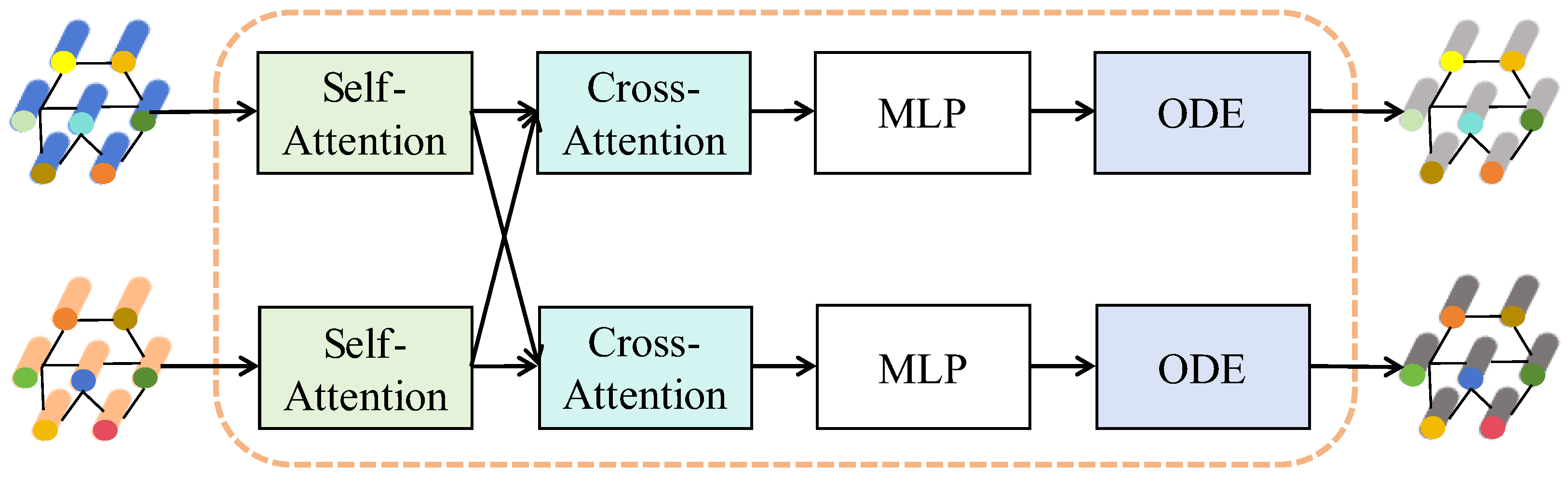
3.3. Graph Diffusion

Traditional graph convolutional networks (GCNs) aggregate information from fixed neighboring nodes, without considering the dynamic and diverse nature of feature information transmission. In contrast, the graph diffusion model allows feature of nodes and adjacency relationships to co-evolve, facilitating more effective information propagation on large-scale sparse graph structures. Thus, we apply the graph diffusion model to the SSL-CD field rather than GCNs. As shown in Figure 2, the figure presents the overall process of the graph diffusion model. After constructing the graph structure, a graph diffusion network [54,55,56] is employed to effectively extract global stable features from irregular regions. First, the bi-temporal graph structures are processed through a self-attention module and a cross-attention module, embedding both structural and feature information of the nodes into a latent space. For instance, consider the graph data $G_1^0$ as follows:

$$G_1^1={\tilde{X}}_1{\Theta }_1{\tilde{X}}_1^T$$

(1)

$$G_1^2=G_1^1{\Theta }_2{G}_2^1$$

(2)

where $G_1^1$ and $G_2^1$ represent the self-attention graphs of $G_1^0$ and $G_2^0$, $G_1^2$ represents the cross-attention graph of $G_1^0$, ${\tilde{X}}_1$ represents the normalized adjacency matrix, and ${\Theta }_1$ and ${\Theta }_2$ are trainable parameters. It is important to note that the cross-attention module effectively integrates features from different time phases, thereby improving the accuracy and robustness. Next, we compute the similarity matrix and encode the similarity matrix with linear layers as follows:

$$\begin{array}{cc}\hfill S_1& =G_1^2{\left(G_1^2\right)}^T\hfill \end{array}$$

(3)

$$\begin{array}{cc}\hfill H_1& =Linea{r}_{\varphi }\left(S_1\right)\hfill \end{array}$$

(4)

where $\varphi$ are the trainable parameters of linear layers.

Following the previously discussed procedures, we represent the node features and positional encodings of the graph as a joint embedding space and extract the high-order features of the bi-temporal graph data. Then, through the graph diffusion process, the features and positions (topological structure) of the nodes co-evolve. The graph diffusion process can be interpreted as a nonlinear filter, where information propagates through neighboring nodes, causing the graph data to diffuse from their initial state to a stable state, in which each connected component equals its average feature. Mathematically, the diffusion process at timescale t can be modeled by the following partial differential equation:

$$\begin{array}{c}\hfill {\displaystyle \frac{\partial {\tilde{z}}_i\left(t\right)}{\partial t}}=div\left({\alpha }_i\left({\mathrm{z}}_i\left(t\right)\right)\nabla {\tilde{z}}_i\left(t\right)\right)\end{array}$$

(5)

where ${\tilde{z}}_i\left(t\right)$ represents the diffusion state of node i from $G_1$ at time t, and ${\alpha }_i$ is a function that controls the diffusion intensity. What we ultimately aim to obtain is the steady-state feature $\tilde{Z}$ after diffusion for time t. Therefore, from the above equation, we have the following:

$$\begin{array}{c}\hfill \tilde{\mathbf{Z}}\left(t\right)=\tilde{\mathbf{Z}}\left(0\right)+{\int }_0^t{\displaystyle \frac{\partial \tilde{\mathbf{Z}}\left(\tau \right)}{\partial \tau }}\mathrm{d}\tau \end{array}$$

(6)

where $\tilde{Z}$(0) represents the initial state, which is the feature H obtained from Equation (4). Then, we introduce a neural ordinary differential equation (ODE) to model the partial differential term in the above equation, using a neural network to parameterize the rate of change of node features:

$$\begin{array}{c}\hfill {\displaystyle \frac{\partial \tilde{\mathbf{Z}}\left(t\right)}{\partial t}}=f(\tilde{\mathbf{Z}}\left(t\right),\tilde{\mathbf{X}},t,\Psi )=(\tilde{\mathbf{X}}-\mathbf{I})\tilde{\mathbf{Z}}\left(t\right)\end{array}$$

(7)

where $\tilde{X}$ represents the normalized adjacency matrix and $\Psi$ gives the trainable parameters. Now, we obtain the steady-state feature after diffusion, which results from the co-evolution of adjacency relationships and feature information in the graph, enabling better capture of the global information of the graph structure.

3.4. Contrastive Learning

Contrastive learning is introduced to drive network training and update the network parameters. Pulling positive examples closer and pushing negative examples farther apart is the main goal of contrastive learning. We designed a fusion contrastive learning strategy, composed of two components, node-level and graph-level components, without the need for data augmentation or random sampling.

For the node level, neighboring nodes in the graph structure are viewed as positive samples, while non-neighboring nodes are viewed as negative samples. This strategy fully utilizes the adjacency information in the graph, avoiding data augmentation for positive samples and random sampling for negative samples. Compared to the strategy used in the PatchSSL method, this strategy is more comprehensive, with positive samples for each sample derived from edge information, rather than solely from image patches corresponding to the same location. Figure 3 shows that sample 2 represents the graph-based contrastive learning sampling strategy, while sample 1 represents the patch-based sampling strategy. From the figure, it is clear that the patch-based sampling strategy only treats patches from the same location as positive samples, while different patches are regarded as negative samples, which does not reflect the characteristics of remote sensing images. However, the graph-based sampling strategy can effectively exploit the distributional consistency in remote sensing images, treating similar nodes as positive samples. For sample 1, the patch-based contrastive learning strategy has only one positive sample from the same area. For sample 2, in the context of the graph-based contrastive learning strategy, the number of positive samples corresponds to the number of its neighboring nodes. During training, this strategy allows the model to efficiently capture the topological relationships between graph nodes. For the graph-level, we followed the strategy of multi-view contrastive learning, treating graph data constructed at different time points as positive samples and pulling them closer together, thereby alleviating the errors introduced by varying imaging conditions. Based on the above sampling strategy, the loss function can be derived:

$$\begin{array}{c}\hfill L=Tr\left({\mathbf{Z}}^{\top }{\mathbf{L}}^{+}\mathbf{Z}\right)-\beta Tr\left({\mathbf{Z}}^{\top }{\mathbf{L}}^{-}\mathbf{Z}\right)+\gamma {∥{\tilde{G}}_1-{\tilde{G}}_2∥}_2^2\end{array}$$

(8)

where $\beta$ and $\gamma$ are non-negative hyperparameters trading off the contrastive terms, $L^{+}$ and $L^{-}$ are the Laplacian matrices of positive samples and negative samples, and ${\tilde{G}}_1$ and ${\tilde{G}}_2$ are the results obtained through the graph diffusion process.

3.5. Change Detection

After obtaining the pre-trained network, the bi-temporal images are input into the network following the procedure outlined above to extract features. The bi-temporal features are then processed using an absolute difference operation to obtain the difference variable, followed by the use of the Otsu thresholding algorithm [57] to generate the final binary change map.

4. Experiments

4.1. Datasets

We employed the datasets from ${\mathrm{S}}^3$Net to evaluate the effectiveness and robustness of our proposed CGD-CD model, and conducted a series of experiments on the following different public datasets: BeiJing, GuangZhou, and Montpellier.

4.1.1. Beijing Dataset

This dataset consists of two RGB optical images, each with dimensions of 500 × 500 pixels and a spatial resolution of 1 m, primarily documenting changes in urban buildings within Beijing. The dataset captures land use changes in Beijing between 2012 and 2013, including residential areas and large warehouses. Due to different imaging conditions, the images exhibit many complicated changes, with buildings and their shadows exhibiting diverse geometric characteristics, making it particularly challenging for analysis. Figure 4 presents a visualization of the Beijing dataset.

4.1.2. Guangzhou Dataset

This dataset consists of a pair of dual-temporal multispectral images, with three channels: red, green, and near-infrared. These images were captured by the SPOT-5 over Guangzhou, primarily reflecting changes in vegetation cover in Guangzhou’s urban areas from October 2006 to October 2007. The images measure 877 × 738 pixels with a spatial resolution of 2.5 m. Due to varying imaging conditions, the vegetation colors in the two images differ, which can easily lead to pseudo-changes during change detection. Figure 5 presents a visualization of the Guangzhou dataset.

4.1.3. Montpellier Dataset

This dataset consists of a pair of images captured by Sentinel-2 on 12 August 2015 and 30 October 2017, over the urban area of Montpellier, with red, green, blue, and near-infrared bands as the bands of interest. The images measure 451 × 426 pixels with a spatial resolution of 10 m, primarily illustrating the growth and changes of the city during urbanization. Due to the low spatial resolution, the images contain relatively complex contextual information, making it prone to false positives during detection. Figure 6 presents a visualization of the Montpellier dataset.

4.2. Evaluation Metrics

The results of the change detection will be shown as a binary map, where white pixels indicate changed areas and black pixels represent unchanged areas. To provide a thorough evaluation of our method’s performance, we utilized five metrics: precision (Pr), recall (Re), F1-score (F1), overall accuracy (OA), and Kappa coefficient (KC). Their definitions are given as follows:

$$\begin{array}{c}\hfill \mathrm{Pr}={\displaystyle \frac{\mathrm{TP}}{\mathrm{TP}+\mathrm{FP}}}\end{array}$$

(9)

$$\begin{array}{c}\hfill \mathrm{Re}={\displaystyle \frac{\mathrm{TP}}{\mathrm{TP}+\mathrm{FN}}}\end{array}$$

(10)

$$\begin{array}{c}\hfill \mathrm{F}1={\displaystyle \frac{2\times \mathrm{Pr}\times \mathrm{Re}}{\mathrm{Pr}+\mathrm{Re}}}\end{array}$$

(11)

$$\begin{array}{c}\hfill \mathrm{OA}={\displaystyle \frac{\mathrm{TP}+\mathrm{TN}}{\mathrm{TP}+\mathrm{TN}+\mathrm{FP}+\mathrm{FN}}}\end{array}$$

(12)

$$\begin{array}{c}\hfill \mathrm{KC}={\displaystyle \frac{\mathrm{OA}-\mathrm{P}}{1-\mathrm{P}}}\end{array}$$

(13)

where,

$$\begin{array}{c}\hfill \mathrm{P}={\displaystyle \frac{(\mathrm{TP}+\mathrm{FP})(\mathrm{TP}+\mathrm{FN})+(\mathrm{FN}+\mathrm{TN})(\mathrm{TP}+\mathrm{FN})}{{(\mathrm{TP}+\mathrm{TN}+\mathrm{FP}+\mathrm{FN})}^2}}\end{array}$$

(14)

where true positive (TP) is the number of pixels that are actually changed and are correctly detected, false positive (FP) is the number of pixels that are actually unchanged but are incorrectly detected as changed, true negative (TN) is the number of pixels that are actually unchanged and are correctly detected, false negative (FN) is the number of pixels that are actually changed but are incorrectly detected.

4.3. Experimental Setting and Baselines

We implemented our framework and performed all experiments in the Pytorch framework with an NVIDIA RTX 3090 GPU, Intel(R) Xeon(R) Platinum 8362 CPU at 2.80 GHz, and 16-GB DDR4 RAM. With a learning rate at 1 × ${10}^{-3}$ and weight decay at 1 × ${10}^{-5}$, the AdamW optimizer was employed. Additionally, the timestep hyperparameter was set to 200. In the training stage, $\beta$ controls the proportion of negative sample loss, while $\gamma$ adjusts the multi-view contrastive loss, and we set $\beta$ to 9 and $\gamma$ to 0.01, respectively. Due to the varying sizes of the datasets, the hyperparameters for kNN algorithm had to be adjusted accordingly. For the Beijing dataset, the hyperparameter k was set to 300; for the Guangzhou dataset, k was set to 750; and for the Montpellier dataset, k was set to 550.

We selected two unsupervised methods and three self-supervised methods as baselines:

• ASEA-CD [58]: The ASEA-CD method gradually expands the adaptive region around each pixel by comparing the spectral similarity between the pixel and its eight neighboring pixels, until no pixel can be found that satisfies the similarity constraint. This method is able to adapt to the shape and size of the target and does not require parameter settings, allowing it to effectively utilize contextual information.
• HyperNet [59]: HyperNet performs full convolutional comparison of multi-temporal spatial and spectral features through a self-supervised learning model, enabling pixel-level feature representation learning. Using the designed spatial and spectral attention branches, along with the novel focal cosine loss function, HyperNet effectively detects changes in hyperspectral images.
• Patch-ssl [40]: The Patch-SSL method is a self-supervised change detection method that views different temporal samples of the same geographical location as positive examples, while samples from different locations are treated as negative examples. This method employs CL to extract informative and discriminative features for change detection.
• ${\mathrm{S}}^3$Net [38]: ${\mathrm{S}}^3$Net introduces the regional consistency principle to generate pseudo-labels for the dataset by checking if image blocks intersect, then uses the pseudo-labels to train the backbone model to generate the change map.

To ensure fairness, all the aforementioned methods were evaluated using the default parameters provided in their respective papers, without any additional post-processing.

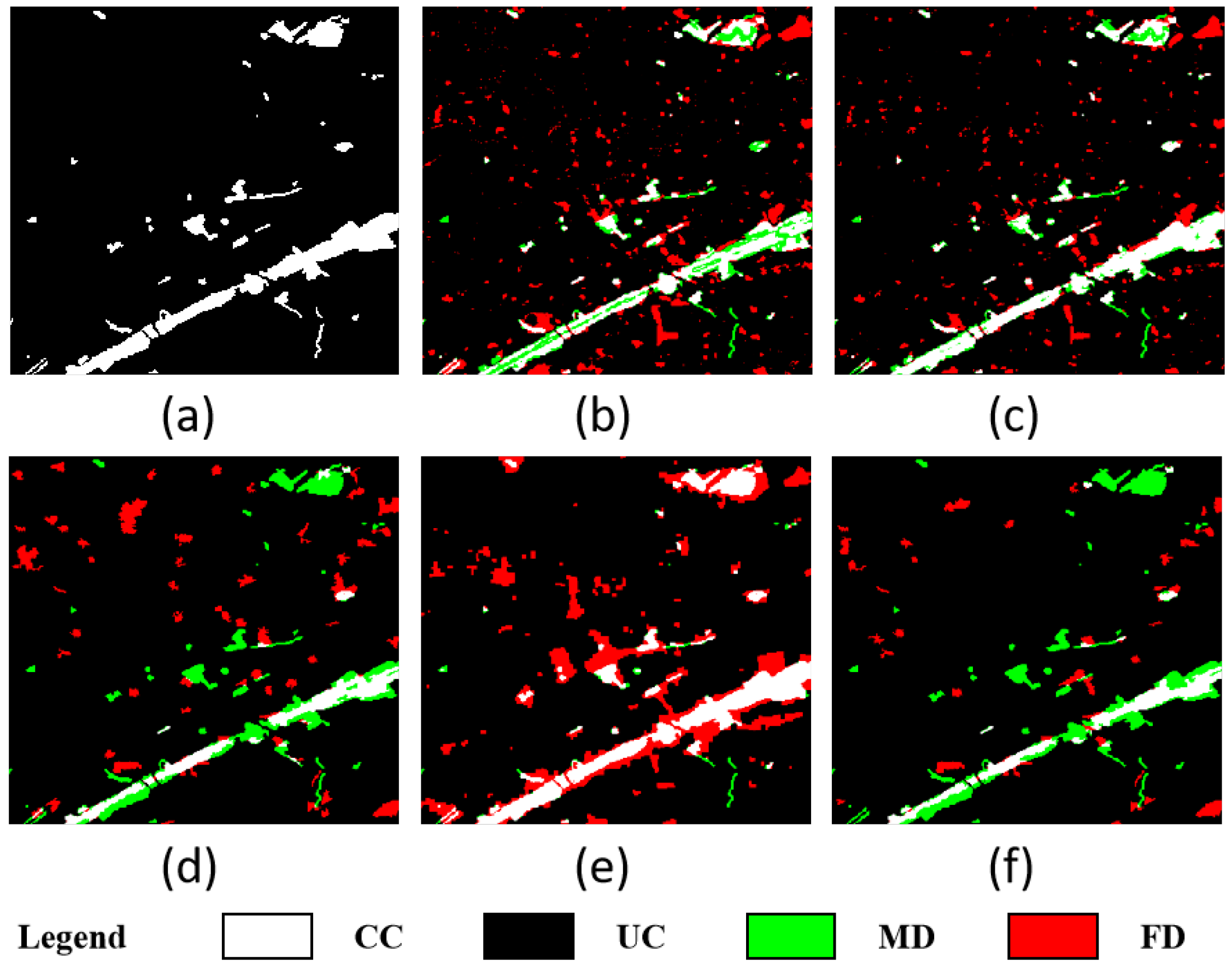
4.4. Comparison Experiments

In this section, we will present the experimental results of our method and the selected comparison methods on three datasets, both qualitatively and quantitatively, using charts. To further illustrate the effectiveness of the proposed method, we will offer detailed explanations of the experimental results. It should be noted that in the comparison visualization of the CD results, white indicates correctly detected changed pixels, black indicates correctly detected unchanged pixels, red represents false positives where pixels were detected as changed but did not actually change, and green represents false negatives where pixels were detected as unchanged but actually changed.

4.4.1. Results on Beijing Dataset

As shown in

Table 1. Quantitative analysis of different methods for Beijing datasets. Best values are in bold.

Datasets	Methods	Pr	Re	F1	OA	KC
Beijing	ASEA-CD	33.5	72.5	45.8	89.5	40.9
	HyperNet	30.9	84.6	45.3	87.6	39.9
	Patch-ssl	26.9	72.4	39.2	93.0	51.7
	${\mathrm{S}}^3$Net	27.7	94.8	42.8	84.6	36.9
	CGD-CD	48.2	76.2	59.1	93.6	55.8

, compared to the other selected change detection (CD) methods, the proposed CGD-CD demonstrates superior overall performance. Our method outperforms the others across most evaluation metrics, especially in the F1 score, where our method achieved the best score of 59.1%. These results indicate that proposed CGD-CD method is more effective at capturing the topological information of remote sensing data, generating better maps of multi-scale change objects.

The visual CD results in Figure 7 also support similar conclusions. Due to the varying imaging conditions in the Beijing dataset, other methods produce results with numerous false positives (excessive red regions). However, in the proposed CGD-CD method, these false positives are effectively suppressed, thanks to the efficient extraction of adjacency information. The results further demonstrate the superiority of CGD-CD in reflecting changes in buildings in the Beijing dataset.

4.4.2. Results on Guangzhou Dataset

The Guangzhou dataset is characterized by a relatively uniform distribution of changes. As shown in

Table 2. Quantitative analysis of different methods for Guangzhou datasets. Best values are in bold.

Datasets	Methods	Pr	Re	F1	OA	KC
Guangzhou	ASEA-CD	95.4	79.7	86.9	96.4	84.8
	HyperNet	59.6	78.9	67.9	88.8	61.3
	Patch-ssl	98.3	72.1	83.2	95.6	80.8
	${\mathrm{S}}^3$Net	97.5	83.4	90.0	96.7	87.1
	CGD-CD	96.6	84.4	90.1	97.2	88.5

, several methods achieve satisfactory performance; however, the proposed method CGD-CD consistently outperforms the others, achieving the best results across all metrics except for the Pr score. Among them, the F1 score reaches 90.1%, which rivals the results of some supervised methods.

In this dataset, pseudo-changes in roads pose a challenge, with most methods misclassifying them due to color variations. However, the proposed method can effectively capture global context, thereby avoiding such misclassifications. The ASEA-CD method, which incorporates context information, performs well on this dataset. However, due to its limited feature representation, it may miss some change information. The Patch-ssl method achieves a Pr score of 98.3%, surpassing our method. This stems from the dataset’s similar cross-temporal distribution. After contrastive learning, the Patch-ssl model becomes more conservative in judging changed features, leading to more missed detections. As seen in the visualization results in Figure 8, it is evident that the proposed method effectively suppresses false changes, and the resulting change detection map aligns more closely with the true distribution of the label data.

4.4.3. Results on Montpellier Dataset

For the Montpellier dataset, which has lower spatial resolution and exhibits greater complexity, extracting change information effectively is challenging. As shown in

Table 3. Quantitative analysis of different methods for Montpellier datasets. Best values are in bold.

Datasets	Methods	Pr	Re	F1	OA	KC
Montpellier	ASEA-CD	46.0	64.9	53.9	92.4	49.9
	HyperNet	59.7	78.7	67.9	93.5	65.2
	Patch-ssl	42.5	39.7	41.1	92.3	36.9
	${\mathrm{S}}^3$Net	43.9	93.7	59.8	91.4	55.7
	CGD-CD	62.4	49.3	70.4	94.2	59.7

, Hypernet achieves the highest score for the Kappa coefficient (65.2%), and ${\mathrm{S}}^3$Net reaches the highest Re score (93.7%), while the proposed CGD-CD model outperforms others in the Pr score (62.4%), F1 score (70.4%), and OA score (94.2%), achieving the best overall detection performance. The visualization results in Figure 9 clearly demonstrate that the proposed method successfully avoids the majority of misclassification errors.

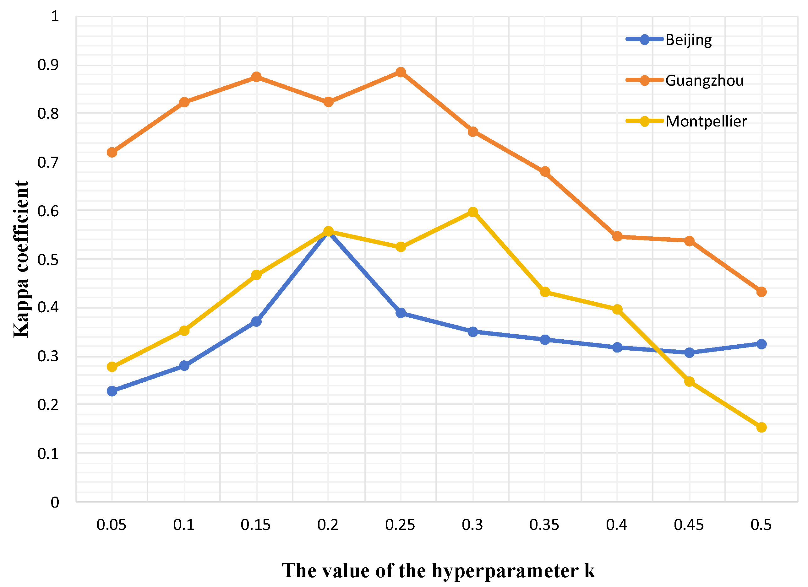
4.5. Parameters Analysis

In the CGD-CD method we proposed, the value of the hyperparameter k plays a crucial role. This parameter is used to construct the adjacency information of the graph. The selection of k must consider both the total number of superpixels (i.e., graph nodes) and the distribution of objects within the data. According to Figure 10, the effect of varying k on the Kappa coefficient across three datasets is illustrated. The figure shows that as k increases, the Kappa coefficient rises to a peak before gradually decreasing. The optimal value of k is achieved when k is set to 0.2–0.3 times the total number of nodes in all three datasets. Therefore, in our experiments, we set k to 0.2 times the total number of nodes. When k is too small, the model becomes excessively sensitive to changes, leading to a high rate of false positives. Conversely, when k is too large, the model fails to adequately detect changes, resulting in missed detections.

4.6. Ablation Study

We conducted a number of thorough ablation tests to evaluate the efficacy of the suggested method, with the results summarized in

Table 4. Ablation experiment of module effectiveness on three datasets. Best values are in bold.

Datasets	GDM	${\mathit{L}}_1$	${\mathit{L}}_2$	OA	KC
Beijing	×	✓	✓	80.9	27.8
	✓	×	✓	85.7	51.2
	✓	✓	×	89.2	47.3
	✓	✓	✓	93.6	55.8
Guangzhou	×	✓	✓	82.7	68.3
	✓	×	✓	95.2	80.4
	✓	✓	×	87.6	69.5
	✓	✓	✓	97.2	88.5
Montpellier	×	✓	✓	67.2	33.5
	✓	×	✓	92.2	36.9
	✓	✓	×	74.1	23.5
	✓	✓	✓	94.2	59.7

. A Graph Convolutional Network (GCN) was used as a backbone to evaluate the effectiveness of the graph diffusion model. The term $L_1$ refers to the contrastive learning loss between nodes, while $L_2$ denotes the multi-view contrastive loss, both of which were employed to validate the necessity of incorporating a fusion-based contrastive learning strategy. For the sake of consistency, all other hyperparameters were kept unchanged during training. As shown in Table 4, changes to the graph diffusion module have the most significant impact on the model. On the Montpellier dataset, the Overall Accuracy (OA) and Kappa values decreased by 27% and 26%, respectively, compared to the proposed model. This suggests that a basic Graph Convolutional Network (GCN) fails to capture robust feature representations on more complex datasets. Experimental data show that the node-based loss function can drive the network to learn high-quality feature vectors, indicating its suitability for graph diffusion networks. However, $L_1$ alone failed to achieve optimal detection performance as it fails to address the inconsistency in graph data from different phases. Thus, introducing $L_2$ is essential, which effectively solves the inconsistency issue and aids the convergence of the overall loss function. Furthermore, the model achieves optimal performance only when both contrastive learning losses are applied simultaneously, thereby confirming the necessity of the proposed fusion contrastive learning strategy.

5. Discussion

5.1. Critical Considerations and Limitations

Although CGD-CD demonstrates excellent performance, it still has some issues and limitations. First, since CGD-CD utilizes SLIC for superpixel segmentation and constructs a graph structure from these superpixels, the superpixel parameter k is set based on individual images. This leads to reduced detection performance when a fixed k value is applied across large datasets, as it cannot dynamically adapt the network’s hidden layer parameters. Moreover, although the model effectively reduces detection degradation caused by false changes, it struggles to extract local detail features in complex scenarios, leading to potential issues such as missing small changes and unclear change boundaries during detection.

5.2. Future Work

In future work, we will explore the introduction of other methods for constructing graphs, such as remapping high-dimensional features before graph reconstruction, to decouple the graph construction process from the network model parameters. Secondly, we will attempt to combine graph neural networks with the DDPM model, training the model to learn more detailed features by progressively removing noise.

6. Conclusions

In this paper, we innovatively introduce a graph diffusion model into the change detection field, enabling the model to fully consider features of objects with varying sizes and contextual information. At the same time, we design a node-level and graph-level combined contrastive learning strategy that brings similar samples closer together, thus improving the model’s capacity to model structure information and reduce false alarms caused by varying imaging conditions. During the inference phase, the absolute difference of the high-quality feature vectors generated by the model is calculated, and the final binary change map is obtained through a thresholding method. The experiments conducted on the selected datasets indicate that the proposed method can achieve optimal comprehensive detection performance, especially in terms of the F1 and OA metrics, which reached maximum values. The detection results on the Guangzhou dataset, with an F1 score of 90.1% and OA score of 97.2%, are comparable to some supervised learning change detection algorithms. The corresponding results indicate that the proposed method not only eliminates the dependence on labeled data but also has high efficiency and effectiveness.

References

1. Jiang, W.; Sun, Y.; Lei, L.; Kuang, G.; Ji, K. Change detection of multisource remote sensing images: A review. Int. J. Digit. Earth 2024, 17, 2398051. [Google Scholar]
2. Cheng, G.; Huang, Y.; Li, X.; Lyu, S.; Xu, Z.; Zhao, H.; Zhao, Q.; Xiang, S. Change detection methods for remote sensing in the last decade: A comprehensive review. Remote Sens. 2024, 16, 2355. [Google Scholar] [CrossRef]
3. Liu, Q.; Wan, S.; Gu, B. A review of the detection methods for climate regime shifts. Discret. Dyn. Nat. Soc. 2016, 2016, 3536183. [Google Scholar]
4. Shi, S.; Zhong, Y.; Zhao, J.; Lv, P.; Liu, Y.; Zhang, L. Land-use/land-cover change detection based on class-prior object-oriented conditional random field framework for high spatial resolution remote sensing imagery. IEEE Trans. Geosci. Remote Sens. 2020, 60, 5600116. [Google Scholar]
5. Coppin, P.; Jonckheere, I.; Nackaerts, K.; Muys, B.; Lambin, E. Review ArticleDigital change detection methods in ecosystem monitoring: A review. Int. J. Remote Sens. 2004, 25, 1565–1596. [Google Scholar]
6. Ridd, M.K.; Liu, J. A comparison of four algorithms for change detection in an urban environment. Remote Sens. Environ. 1998, 63, 95–100. [Google Scholar]
7. Liu, Y.; Pang, C.; Zhan, Z.; Zhang, X.; Yang, X. Building change detection for remote sensing images using a dual-task constrained deep siamese convolutional network model. IEEE Geosci. Remote Sens. Lett. 2020, 18, 811–815. [Google Scholar]
8. Luo, H.; Liu, C.; Wu, C.; Guo, X. Urban change detection based on Dempster–Shafer theory for multitemporal very high-resolution imagery. Remote Sens. 2018, 10, 980. [Google Scholar] [CrossRef]
9. Brunner, D.; Bruzzone, L.; Lemoine, G. Change detection for earthquake damage assessment in built-up areas using very high resolution optical and SAR imagery. In Proceedings of the 2010 IEEE International Geoscience and Remote Sensing Symposium, Honolulu, HI, USA, 25–30 July 2010; pp. 3210–3213. [Google Scholar]
10. Hamidi, E.; Peter, B.G.; Muñoz, D.F.; Moftakhari, H.; Moradkhani, H. Fast flood extent monitoring with SAR change detection using google earth engine. IEEE Trans. Geosci. Remote Sens. 2023, 61, 4201419. [Google Scholar]
11. He, X.; Zhang, S.; Xue, B.; Zhao, T.; Wu, T. Cross-modal change detection flood extraction based on convolutional neural network. Int. J. Appl. Earth Obs. Geoinf. 2023, 117, 103197. [Google Scholar]
12. Khelifi, L.; Mignotte, M. Deep learning for change detection in remote sensing images: Comprehensive review and meta-analysis. IEEE Access 2020, 8, 126385–126400. [Google Scholar] [CrossRef]
13. Bai, T.; Wang, L.; Yin, D.; Sun, K.; Chen, Y.; Li, W.; Li, D. Deep learning for change detection in remote sensing: A review. Geo-Spat. Inf. Sci. 2023, 26, 262–288. [Google Scholar] [CrossRef]
14. Zhang, M.; Xu, G.; Chen, K.; Yan, M.; Sun, X. Triplet-Based Semantic Relation Learning for Aerial Remote Sensing Image Change Detection. IEEE Geosci. Remote Sens. Lett. 2019, 16, 266–270. [Google Scholar] [CrossRef]
15. Daudt, R.C.; Le Saux, B.; Boulch, A. Fully convolutional siamese networks for change detection. In Proceedings of the 2018 25th IEEE International Conference on Image Processing (ICIP), Athens, Greece, 7–10 October 2018; pp. 4063–4067. [Google Scholar]
16. Lei, T.; Wang, J.; Ning, H.; Wang, X.; Xue, D.; Wang, Q.; Nandi, A.K. Difference enhancement and spatial–spectral nonlocal network for change detection in VHR remote sensing images. IEEE Trans. Geosci. Remote Sens. 2021, 60, 4507013. [Google Scholar] [CrossRef]
17. Liu, X.; Zhang, F.; Hou, Z.; Mian, L.; Wang, Z.; Zhang, J.; Tang, J. Self-supervised learning: Generative or contrastive. IEEE Trans. Knowl. Data Eng. 2021, 35, 857–876. [Google Scholar] [CrossRef]
18. He, K.; Fan, H.; Wu, Y.; Xie, S.; Girshick, R. Momentum contrast for unsupervised visual representation learning. In Proceedings of the IEEE/CVF Conference on Computer Vision and Pattern Recognition, Seattle, WA, USA, 13–19 June 2020; pp. 9729–9738. [Google Scholar]
19. Chen, T.; Kornblith, S.; Norouzi, M.; Hinton, G. A simple framework for contrastive learning of visual representations. In Proceedings of the International Conference on Machine Learning, Virtual, 13–18 July 2020; pp. 1597–1607. [Google Scholar]
20. Grill, J.B.; Strub, F.; Altché, F.; Tallec, C.; Richemond, P.; Buchatskaya, E.; Doersch, C.; Avila Pires, B.; Guo, Z.; Gheshlaghi Azar, M.; et al. Bootstrap your own latent-a new approach to self-supervised learning. Adv. Neural Inf. Process. Syst. 2020, 33, 21271–21284. [Google Scholar]
21. Chen, X.; He, K. Exploring simple siamese representation learning. In Proceedings of the IEEE/CVF Conference on Computer Vision and Pattern Recognition, Nashville, TN, USA, 20–25 June 2021; pp. 15750–15758. [Google Scholar]
22. Saha, S.; Ebel, P.; Zhu, X.X. Self-Supervised Multisensor Change Detection. IEEE Trans. Geosci. Remote Sens. 2022, 60, 4405710. [Google Scholar] [CrossRef]
23. Qu, Y.; Li, J.; Huang, X.; Wen, D. TD-SSCD: A novel network by fusing temporal and differential information for self-supervised remote sensing image change detection. IEEE Trans. Geosci. Remote Sens. 2023, 61, 5407015. [Google Scholar] [CrossRef]
24. Chen, Y.; Bruzzone, L. Self-supervised change detection by fusing SAR and optical multi-temporal images. In Proceedings of the 2021 IEEE International Geoscience and Remote Sensing Symposium IGARSS, Brussels, Belgium, 11–16 July 2021; pp. 3101–3104. [Google Scholar]
25. Chen, Y.; Bruzzone, L. A self-supervised approach to pixel-level change detection in bi-temporal RS images. IEEE Trans. Geosci. Remote Sens. 2022, 60, 4413911. [Google Scholar] [CrossRef]
26. Jian, P.; Ou, Y.; Chen, K. Hypergraph Self-Supervised Learning-Based Joint Spectral-Spatial-Temporal Feature Representation for Hyperspectral Image Change Detection. IEEE J. Sel. Top. Appl. Earth Obs. Remote Sens. 2025, 18, 741–756. [Google Scholar] [CrossRef]
27. Wan, R.; Zhang, J.; Huang, Y.; Li, Y.; Hu, B.; Wang, B. Leveraging Diffusion Modeling for Remote Sensing Change Detection in Built-Up Urban Areas. IEEE Access 2024, 12, 7028–7039. [Google Scholar] [CrossRef]
28. Tian, J.; Lei, J.; Zhang, J.; Xie, W.; Li, Y. SwiMDiff: Scene-Wide Matching Contrastive Learning With Diffusion Constraint for Remote Sensing Image. IEEE Trans. Geosci. Remote Sens. 2024, 62, 5613213. [Google Scholar] [CrossRef]
29. Ho, J.; Jain, A.; Abbeel, P. Denoising diffusion probabilistic models. Adv. Neural Inf. Process. Syst. 2020, 33, 6840–6851. [Google Scholar]
30. Song, Y.; Ermon, S. Generative modeling by estimating gradients of the data distribution. arXiv 2019, arXiv:1907.05600. [Google Scholar]
31. Song, Y.; Sohl-Dickstein, J.; Kingma, D.P.; Kumar, A.; Ermon, S.; Poole, B. Score-based generative modeling through stochastic differential equations. arXiv 2020, arXiv:2011.13456. [Google Scholar]
32. Goodfellow, I.; Pouget-Abadie, J.; Mirza, M.; Xu, B.; Warde-Farley, D.; Ozair, S.; Courville, A.; Bengio, Y. Generative adversarial networks. Commun. ACM 2020, 63, 139–144. [Google Scholar] [CrossRef]
33. Dhariwal, P.; Nichol, A. Diffusion models beat gans on image synthesis. Adv. Neural Inf. Process. Syst. 2021, 34, 8780–8794. [Google Scholar]
34. Xiang, W.; Yang, H.; Huang, D.; Wang, Y. Denoising diffusion autoencoders are unified self-supervised learners. In Proceedings of the IEEE/CVF International Conference on Computer Vision, Paris, France, 1–6 October 2023; pp. 15802–15812. [Google Scholar]
35. Chen, X.; Liu, Z.; Xie, S.; He, K. Deconstructing denoising diffusion models for self-supervised learning. arXiv 2024, arXiv:2401.14404. [Google Scholar]
36. Liu, Y.; Yue, J.; Xia, S.; Ghamisi, P.; Xie, W.; Fang, L. Diffusion Models Meet Remote Sensing: Principles, Methods, and Perspectives. IEEE Trans. Geosci. Remote Sens. 2024, 62, 4708322. [Google Scholar] [CrossRef]
37. Bandara, W.G.C.; Nair, N.G.; Patel, V.M. Ddpm-cd: Remote sensing change detection using denoising diffusion probabilistic models. arXiv 2022, arXiv:2206.11892. [Google Scholar]
38. Zhan, T.; Gong, M.; Jiang, X.; Zhang, E. S 3 Net: Superpixel-Guided Self-Supervised Learning Network for Multitemporal Image Change Detection. IEEE Geosci. Remote Sens. Lett. 2023, 20, 5002205. [Google Scholar]
39. Alvarez, J.L.H.; Ravanbakhsh, M.; Demir, B. S2-cGAN: Self-supervised adversarial representation learning for binary change detection in multispectral images. In Proceedings of the IGARSS 2020—2020 IEEE International Geoscience and Remote Sensing Symposium, Waikoloa, HI, USA, 26 September–2 October 2020; pp. 2515–2518. [Google Scholar]
40. Chen, Y.; Bruzzone, L. Self-Supervised Change Detection in Multiview Remote Sensing Images. IEEE Trans. Geosci. Remote Sens. 2022, 60, 5402812. [Google Scholar] [CrossRef]
41. Gong, M.; Zhou, H.; Qin, A.K.; Liu, W.; Zhao, Z. Self-paced co-training of graph neural networks for semi-supervised node classification. IEEE Trans. Neural Netw. Learn. Syst. 2022, 34, 9234–9247. [Google Scholar]
42. Fan, X.; Gong, M.; Xie, Y.; Jiang, F.; Li, H. Structured self-attention architecture for graph-level representation learning. Pattern Recognit. 2020, 100, 107084. [Google Scholar]
43. Jian, P.; Ou, Y.; Chen, K. Uncertainty-Aware Graph Self-Supervised Learning for Hyperspectral Image Change Detection. IEEE Trans. Geosci. Remote Sens. 2024, 62, 5509019. [Google Scholar] [CrossRef]
44. Liu, J.; Chen, K.; Xu, G.; Li, H.; Yan, M.; Diao, W.; Sun, X. Semi-Supervised Change Detection Based on Graphs with Generative Adversarial Networks. In Proceedings of the IGARSS 2019—2019 IEEE International Geoscience and Remote Sensing Symposium, Yokohama, Japan, 28 July–2 August 2019; pp. 74–77. [Google Scholar] [CrossRef]
45. Wu, J.; Li, B.; Qin, Y.; Ni, W.; Zhang, H.; Fu, R.; Sun, Y. A multiscale graph convolutional network for change detection in homogeneous and heterogeneous remote sensing images. Int. J. Appl. Earth Obs. Geoinf. 2021, 105, 102615. [Google Scholar]
46. Shuai, W.; Jiang, F.; Zheng, H.; Li, J. MSGATN: A superpixel-based multi-scale Siamese graph attention network for change detection in remote sensing images. Appl. Sci. 2022, 12, 5158. [Google Scholar] [CrossRef]
47. Nichol, A.; Dhariwal, P.; Ramesh, A.; Shyam, P.; Mishkin, P.; McGrew, B.; Sutskever, I.; Chen, M. Glide: Towards photorealistic image generation and editing with text-guided diffusion models. arXiv 2021, arXiv:2112.10741. [Google Scholar]
48. Ramesh, A.; Dhariwal, P.; Nichol, A.; Chu, C.; Chen, M. Hierarchical text-conditional image generation with clip latents. arXiv 2022, arXiv:2204.06125. [Google Scholar]
49. Baranchuk, D.; Rubachev, I.; Voynov, A.; Khrulkov, V.; Babenko, A. Label-Efficient Semantic Segmentation with Diffusion Models. arXiv 2022, arXiv:2112.03126. [Google Scholar]
50. Ma, Y.; Zhan, K. Self-Contrastive Graph Diffusion Network. In Proceedings of the 31st ACM International Conference on Multimedia, Ottawa, ON, Canada, 29 October–3 November 2023; pp. 3857–3865. [Google Scholar]
51. Wen, Y.; Ma, X.; Zhang, X.; Pun, M.O. GCD-DDPM: A generative change detection model based on difference-feature guided DDPM. IEEE Trans. Geosci. Remote Sens. 2024, 62, 5404416. [Google Scholar]
52. Ding, X.; Qu, J.; Dong, W.; Zhang, T.; Li, N.; Yang, Y. Graph Representation Learning-Guided Diffusion Model for Hyperspectral Change Detection. IEEE Geosci. Remote Sens. Lett. 2024, 21, 5506405. [Google Scholar] [CrossRef]
53. Achanta, R.; Shaji, A.; Smith, K.; Lucchi, A.; Fua, P.; Süsstrunk, S. SLIC superpixels compared to state-of-the-art superpixel methods. IEEE Trans. Pattern Anal. Mach. Intell. 2012, 34, 2274–2282. [Google Scholar]
54. Chamberlain, B.; Rowbottom, J.; Eynard, D.; Di Giovanni, F.; Dong, X.; Bronstein, M. Beltrami flow and neural diffusion on graphs. Adv. Neural Inf. Process. Syst. 2021, 34, 1594–1609. [Google Scholar]
55. Chamberlain, B.; Rowbottom, J.; Gorinova, M.I.; Bronstein, M.; Webb, S.; Rossi, E. Grand: Graph neural diffusion. In Proceedings of the International Conference on Machine Learning, Virtual, 18–24 July 2021; pp. 1407–1418. [Google Scholar]
56. Chen, Q.; Wang, Y.; Wang, Y.; Yang, J.; Lin, Z. Optimization-induced graph implicit nonlinear diffusion. In Proceedings of the International Conference on Machine Learning, Baltimore, MD, USA, 17–23 July 2022; pp. 3648–3661. [Google Scholar]
57. Otsu, N. A threshold selection method from gray-level histograms. Automatica 1975, 11, 23–27. [Google Scholar]
58. Lv, Z.; Wang, F.; Liu, T.; Kong, X.; Benediktsson, J.A. Novel Automatic Approach for Land Cover Change Detection by Using VHR Remote Sensing Images. IEEE Geosci. Remote Sens. Lett. 2022, 19, 8016805. [Google Scholar] [CrossRef]
59. Hu, M.; Wu, C.; Zhang, L. HyperNet: Self-Supervised Hyperspectral Spatial–Spectral Feature Understanding Network for Hyperspectral Change Detection. IEEE Trans. Geosci. Remote Sens. 2022, 60, 5543017. [Google Scholar] [CrossRef]
Figure 1. Overall architecture of the proposed CGD-CD method, which constructs a dual-branch CD network with the graph diffusion model to fully extract the steady-state features and global spatial features of dual-temporal images, in order to improve the differentiation between the changed and unchanged regions. SLIC stands for simple linear iterative clustering.
Remotesensing 17 01144 g001
Figure 2. Architecture of the graph diffusion model. MLP refers to MultiLayer Perceptron, and ODE represents the Ordinary Differential Equation solver. The dual-temporal graph data are first passed through the self-attention and cross-attention modules to extract high-level features across temporal phases. After undergoing a diffusion process for t time steps, the steady-state diffusion features are finally obtained through a parameterized neural ODE solver, where t is a tunable parameter.
Remotesensing 17 01144 g002
Figure 3. Intuitive comparison based on different sampling strategies. Sample 1 represents patch-based sampling strategy, and sample 2 represents graph node-based sampling strategy. The arrow indicates that the referenced node is adjacent to node 2.
Remotesensing 17 01144 g003
Figure 4. Beijing dataset: (a) Pre-event image. (b) Post-event image. (c) Reference image.
Remotesensing 17 01144 g004
Figure 5. Guangzhou dataset: (a) Pre-event image. (b) Post-event image. (c) Reference image.
Remotesensing 17 01144 g005
Figure 6. Montpellier dataset: (a) Pre-event image. (b) Post-event image. (c) Reference image.
Remotesensing 17 01144 g006
Figure 7. The results obtained by each method on the Beijing dataset. (a) Ground-truth map. (b) ASEA-CD. (c) HyperNet. (d) Patch-ssl. (e) S 3 Net. (f) CGD-CD. (CC indicates correctly changed pixels, UC indicates unchanged pixels, MD represents missed detection, and FD represents false detection).
Remotesensing 17 01144 g007
Figure 8. The results obtained by each method on the Guangzhou dataset. (a) Ground-truth map. (b) ASEA-CD. (c) HyperNet. (d) Patch-ssl. (e) S 3 Net. (f) CGD-CD. (CC indicates correctly changed pixels, UC indicates unchanged pixels, MD represents missed detection, and FD represents false detection).
Remotesensing 17 01144 g008
Figure 9. The results obtained by each method on the Montpellier dataset. (a) Ground-truth map. (b) ASEA-CD. (c) HyperNet. (d) Patch-ssl. (e) S 3 Net. (f) CGD-CD. (CC indicates correctly changed pixels, UC indicates unchanged pixels, MD represents missed detection, and FD represents false detection).
Remotesensing 17 01144 g009
Figure 10. Relationship between KC and ratio of k on different datasets.
Remotesensing 17 01144 g010