

Spatiotemporal Vegetation Dynamics, Forest Loss, and Recovery: Multidecadal Analysis of the U.S. Triple Crown National Scenic Trail Network


Abstract

1. Introduction
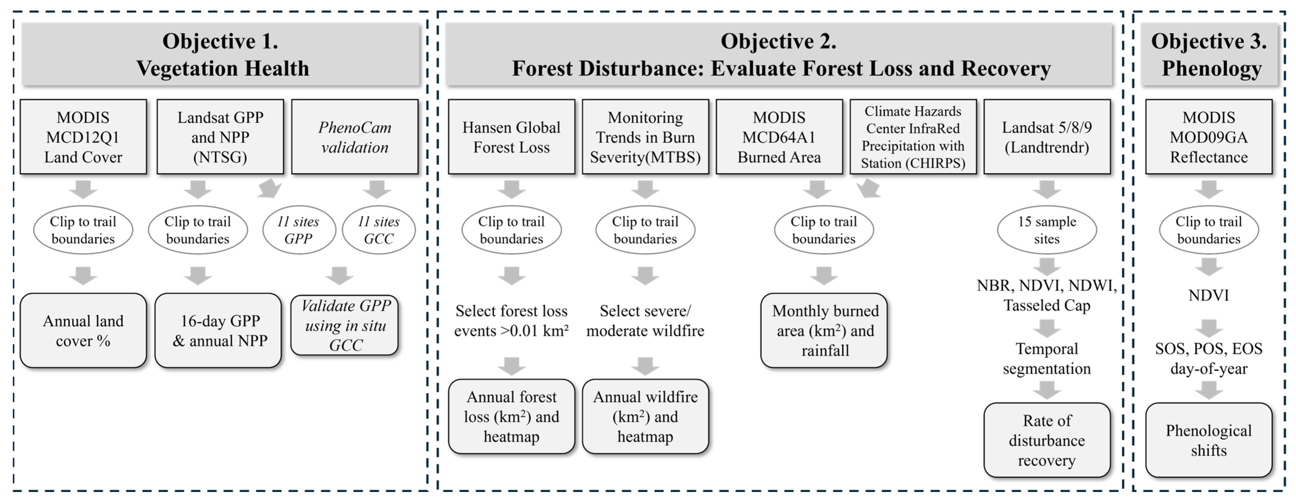
2. Methods
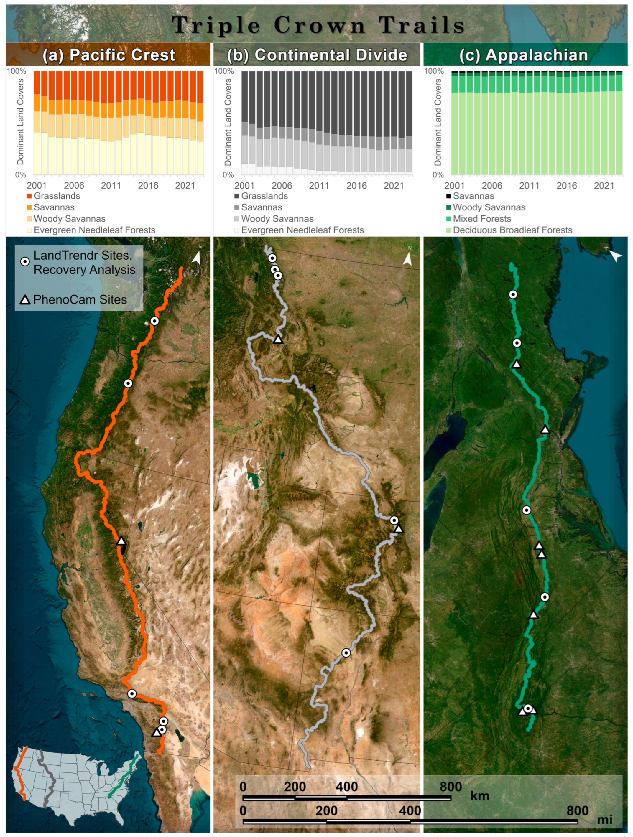
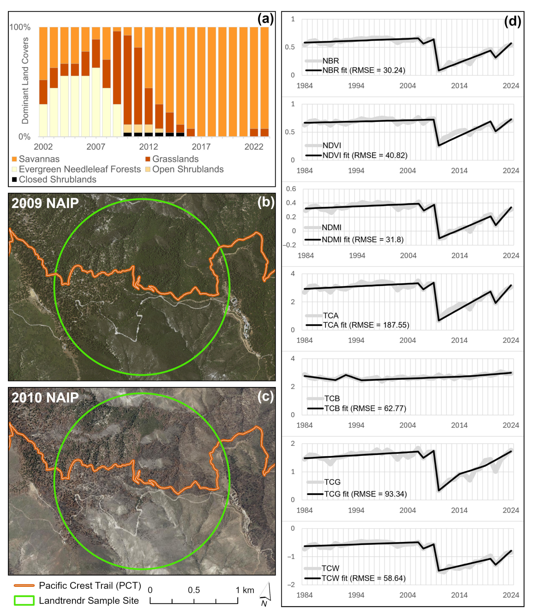
2.1. Study Site
2.2. Vegetation Health
2.3. Forest Loss Severity and Recovery
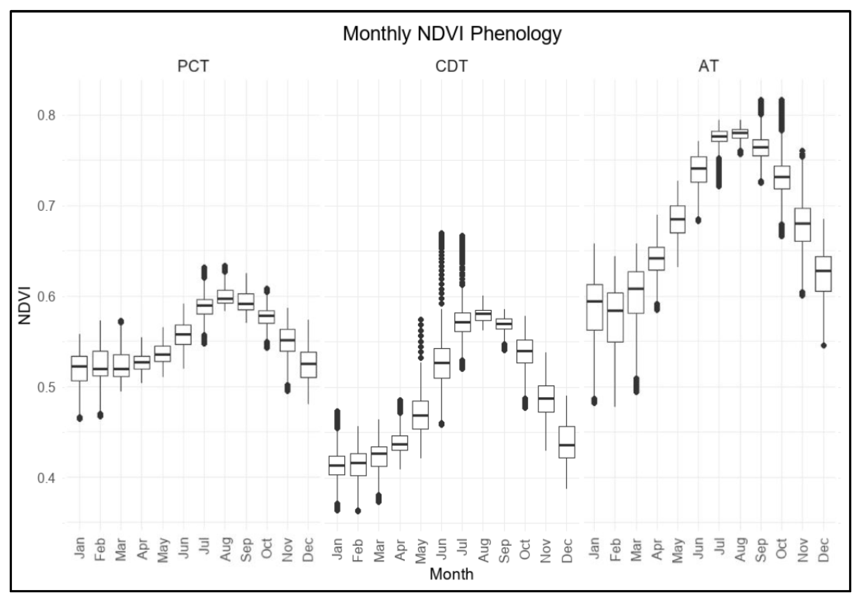
2.4. Phenology
3. Results
3.1. Vegetation Health
3.1.1. Forest Productivity
3.1.2. PhenoCam Validation
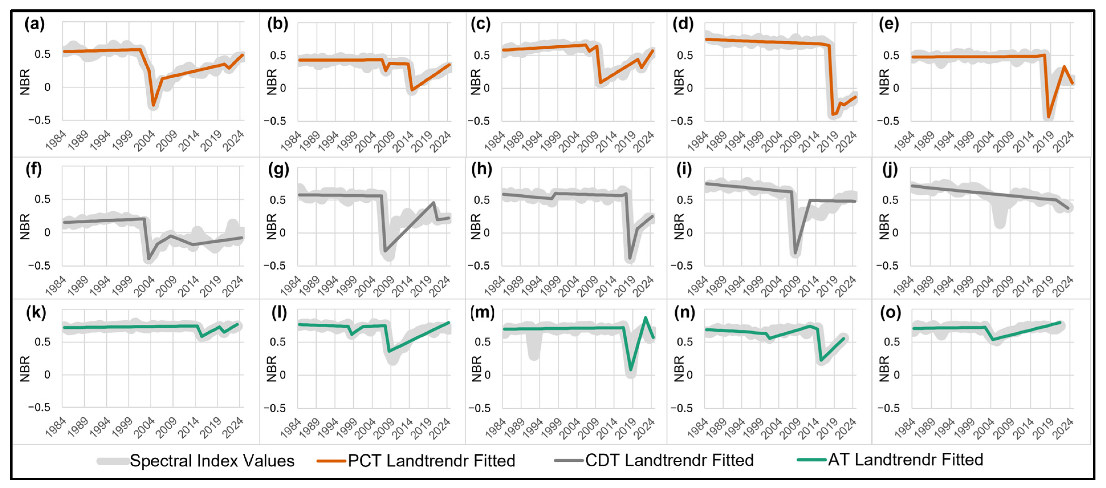
3.2. Forest Loss Severity and Recovery
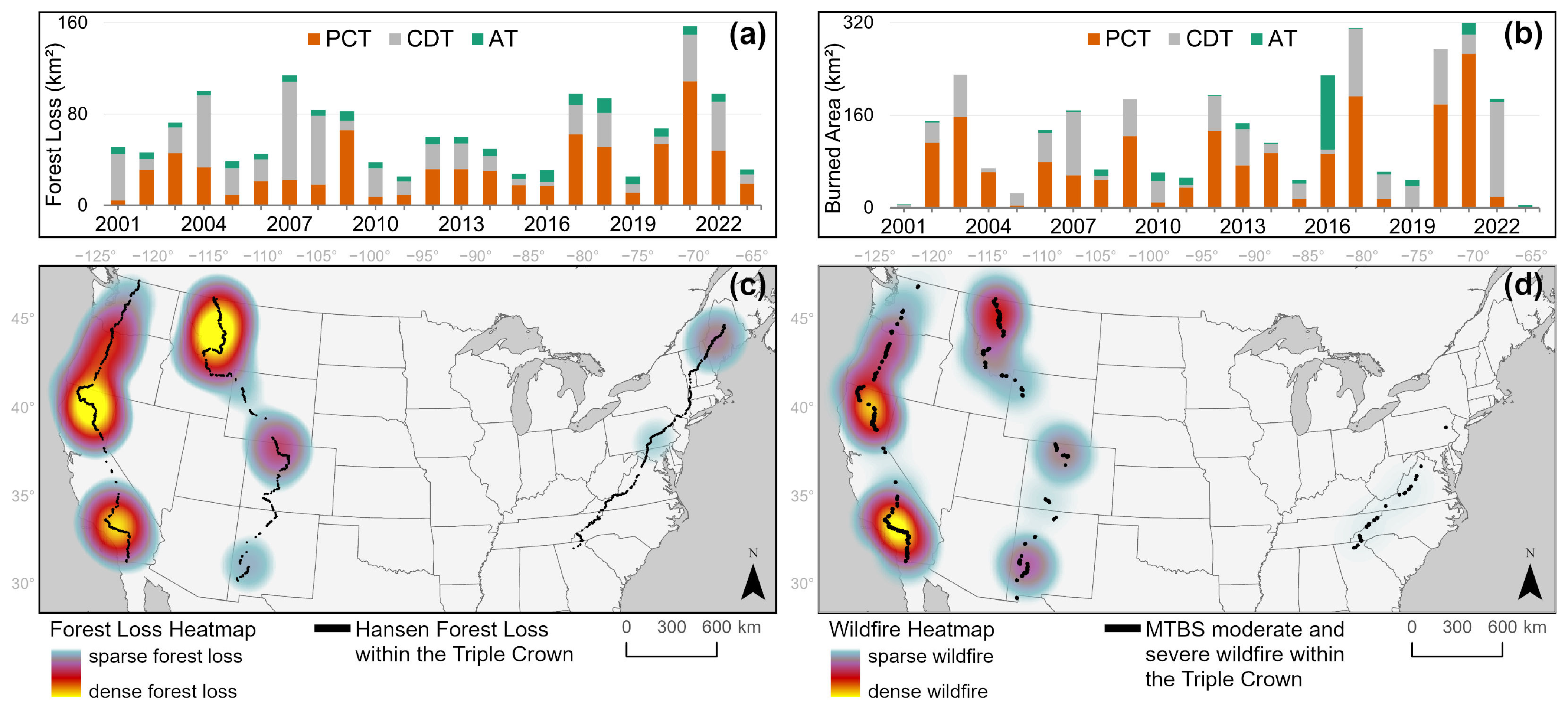
3.2.1. Forest Loss
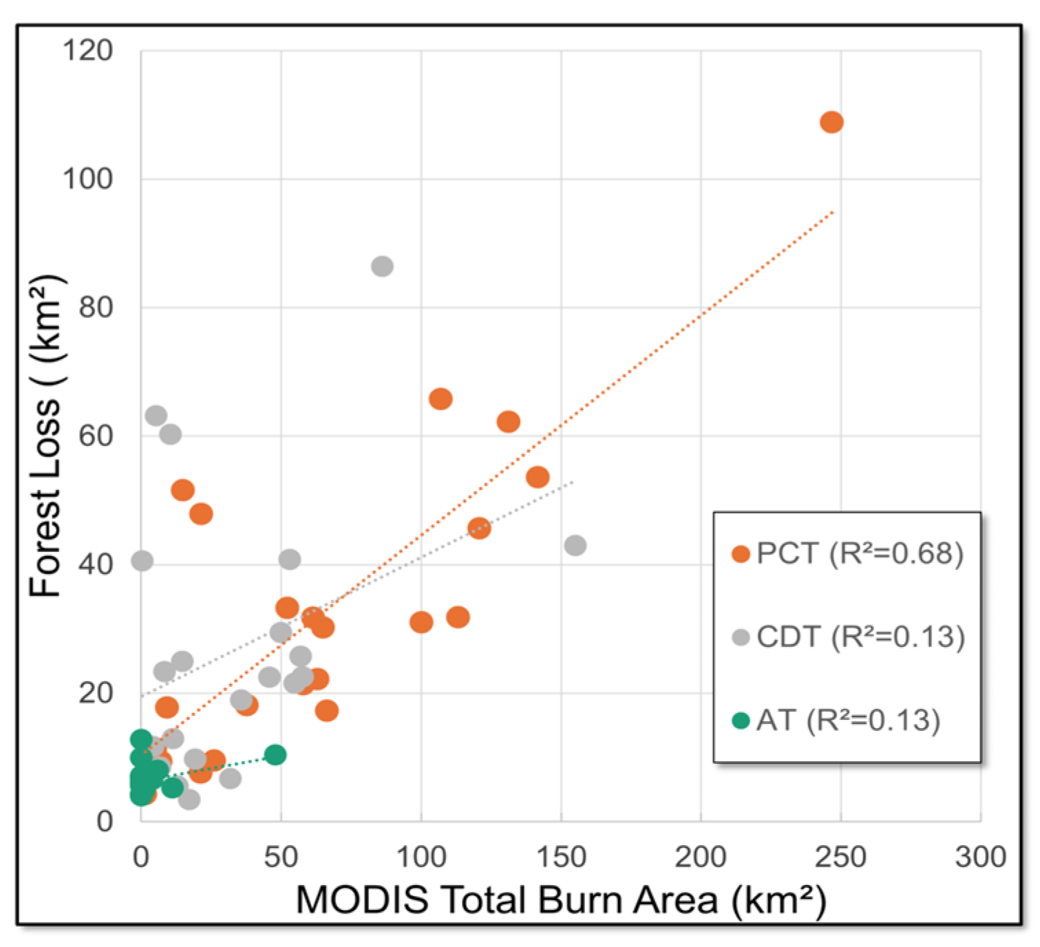
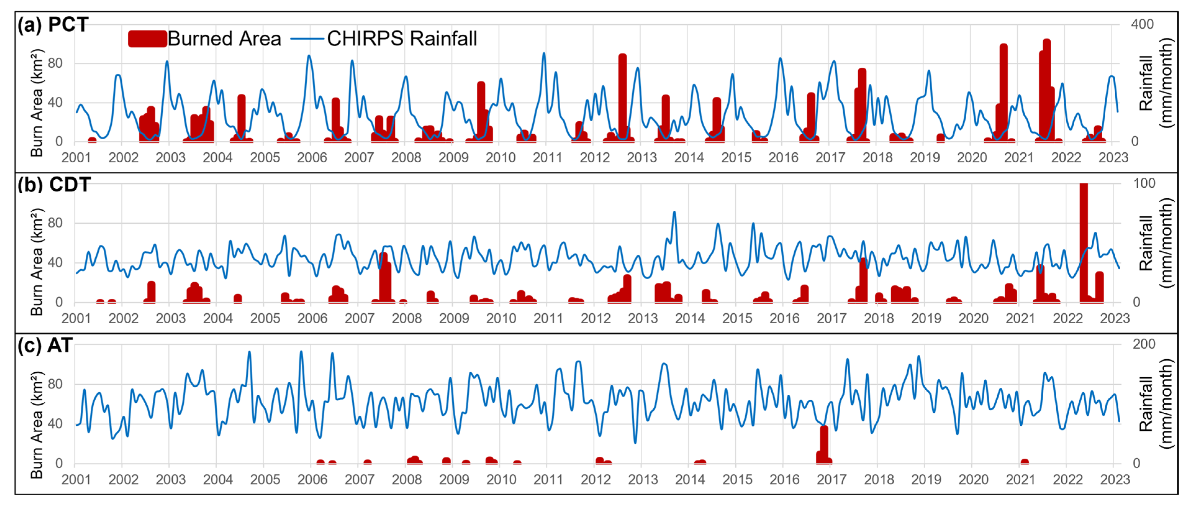
3.2.2. Wildfire
3.2.3. Recovery
3.3. Phenology
4. Discussion
5. Conclusions
Author Contributions
Funding
Data Availability Statement
Acknowledgments
Conflicts of Interest
References
- National Trails System Act, 1968. Public Law 90–543-OCT. 2. Available online: https://www.govinfo.gov/content/pkg/STATUTE-82/pdf/STATUTE-82-Pg919.pdf (accessed on 12 January 2025).
- Cerveny, L.; Derrien, M.; Miller, A.B. Shared Stewardship and National Scenic Trails: Building on a Legacy of Partnerships. Int. J. Wilderness 2020, 26, 18–33. [Google Scholar]
- Dieffenbach, F. Appalachian National Scenic Trail Vital Signs Monitoring Plan; Natural Resource Program Center, Ed.; Natural resources report; U.S. Department of the Interior, National Park Service, Natural Resource Program Center: Fort Collins, CO, USA, 2011. [Google Scholar]
- Tourville, J.C.; Murray, G.L.D.; Nelson, S.J. Distinct Latitudinal Patterns of Shifting Spring Phenology across the Appalachian Trail Corridor. Ecology 2024, 105, e4403. [Google Scholar] [CrossRef] [PubMed]
- Meng, R.; Gao, R.; Zhao, F.; Huang, C.; Sun, R.; Lv, Z.; Huang, Z. Landsat-Based Monitoring of Southern Pine Beetle Infestation Severity and Severity Change in a Temperate Mixed Forest. Remote Sens. Environ. 2022, 269, 112847. [Google Scholar] [CrossRef]
- Ye, S.; Rogan, J.; Zhu, Z.; Hawbaker, T.J.; Hart, S.J.; Andrus, R.A.; Meddens, A.J.H.; Hicke, J.A.; Eastman, J.R.; Kulakowski, D. Detecting Subtle Change from Dense Landsat Time Series: Case Studies of Mountain Pine Beetle and Spruce Beetle Disturbance. Remote Sens. Environ. 2021, 263, 112560. [Google Scholar] [CrossRef]
- Kantola, T.; Lyytikäinen-Saarenmaa, P.; Coulson, R.; Holopainen, M.; Tchakerian, M.; Streett, D. Development of Monitoring Methods for Hemlock Woolly Adelgid Induced Tree Mortality within a Southern Appalachian Landscape with Inhibited Access. IForest Biogeosciences For. 2016, 9, 178–186. [Google Scholar] [CrossRef]
- Meng, R.; Dennison, P.E.; Huang, C.; Moritz, M.A.; D’Antonio, C. Effects of Fire Severity and Post-Fire Climate on Short-Term Vegetation Recovery of Mixed-Conifer and Red Fir Forests in the Sierra Nevada Mountains of California. Remote Sens. Environ. 2015, 171, 311–325. [Google Scholar] [CrossRef]
- McKinley, P.S.; Belote, R.T.; Aplet, G.H. An Assessment of Ecological Values and Conservation Gaps in Protection beyond the Corridor of the Appalachian Trail. Conserv. Sci. Pract. 2019, 1, e30. [Google Scholar] [CrossRef]
- Wilson, M.B.; Belote, R.T. The Value of Trail Corridors for Bold Conservation Planning. Land 2022, 11, 348. [Google Scholar] [CrossRef]
- Simpson, L. National Scenic and Historic Trails: Inventory, Assessment, and Monitoring; U.S. Department of the Interior, Bureau of Land Management, National Conservation Lands Division: Washington, DC, USA, 2020. [Google Scholar]
- Hop, K.D.; Strassman, A.C.; Hall, M.; Menard, S.; Largay, E.; Sattler, S.; Hoy, E.E.; Ruhser, J.; Hlavacek, E.; Dieck, J. National Park Service Vegetation Mapping Inventory Program: Appalachian National Scenic Trail Vegetation Mapping Project; Natural Resource Report; National Park Service: Fort Collins, CO, USA, 2017. [Google Scholar]
- Burns, D.A.; McDonnell, T.C.; Rice, K.C.; Lawrence, G.B.; Sullivan, T.J. Chronic and Episodic Acidification of Streams along the Appalachian Trail Corridor, Eastern United States. Hydrol. Process. 2020, 34, 1498–1513. [Google Scholar] [CrossRef]
- Clark, J.; Wang, Y.; August, P.V. Assessing Current and Projected Suitable Habitats for Tree-of-Heaven along the Appalachian Trail. Philos. Trans. R. Soc. B Biol. Sci. 2014, 369, 20130192. [Google Scholar] [CrossRef]
- Jobe, J.T.; Briggs, R.; Gold, R.; DeLong, S.; Hille, M.; Delano, J.; Johnstone, S.A.; Pickering, A.; Phillips, R.; Calvert, A.T. The Pondosa Fault Zone: A Distributed Dextral-Normal-Oblique Fault System in Northeastern California, USA. Geosphere 2023, 19, 179–205. [Google Scholar] [CrossRef]
- Rockwell, B.W. Description and Validation of an Automated Methodology for Mapping Mineralogy, Vegetation, and Hydrothermal Alteration Type from ASTER Satellite Imagery with Examples from the San Juan Mountains, Colorado; U.S. Geological Survey: Reston, VA, USA, 2012. [Google Scholar]
- Continental Divide National Scenic Trail Comprehensive Plan; FSM 2350. Available online: https://www.federalregister.gov/documents/2009/10/05/E9-23873/continental-divide-national-scenic-trail-comprehensive-plan-fsm-2350 (accessed on 12 January 2025).
- Lindley, S.M.; Wilkins, E.J.; Farley, C.; Rogers, K.; Schuster, R. Delineating Draft Inventory Analysis Units for National Scenic and Historic Trails Inventory, Assessment, and Monitoring Programs; Scientific Investigations Report; USGS: Reston, VA, USA, 2024. [Google Scholar]
- Gross, J.; Hansen, R.; Goetz, S.; Theobald, D.; Melton, F.; Piekielek, N.; Nemani, R. Remote Sensing for Inventory and Monitoring of U.S. National Parks. In Remote Sensing of Protected Lands; Remote Sensing Applications Series; CRC Press: Boca Raton, FL, USA, 2011; Volume 20114962, pp. 29–56. ISBN 978-1-4398-4187-7. [Google Scholar]
- Wang, Y.; Lu, Z.; Sheng, Y.; Zhou, Y. Remote Sensing Applications in Monitoring of Protected Areas. Remote Sens. 2020, 12, 1370. [Google Scholar] [CrossRef]
- Clark, S.G.; Hohl, A.M.; Picard, C.H.; Thomas, E. Large-Scale Conservation in the Common Interest; Springer: Cham, Switzerland, 2015; ISBN 978-3-319-07419-1. [Google Scholar]
- Wang, Y.; Mitchell, B.R.; Nugranad-Marzilli, J.; Bonynge, G.; Zhou, Y.; Shriver, G. Remote Sensing of Land-Cover Change and Landscape Context of the National Parks: A Case Study of the Northeast Temperate Network. Remote Sens. Environ. 2009, 113, 1453–1461. [Google Scholar] [CrossRef]
- Darabi, H.; Haghighi, A.T.; Klöve, B.; Luoto, M. Remote Sensing of Vegetation Trends: A Review of Methodological Choices and Sources of Uncertainty. Remote Sens. Appl. Soc. Environ. 2025, 37, 101500. [Google Scholar] [CrossRef]
- Zhang, J.; Yang, Z.; Zheng, S.; Yue, H. Dynamic Monitoring of Vegetation Growth in Engebei Ecological Demonstration Area Based on Remote Sensing. Environ. Earth Sci. 2024, 83, 59. [Google Scholar] [CrossRef]
- Pradhan, B.; Yoon, S.; Lee, S. Examining the Dynamics of Vegetation in South Korea: An Integrated Analysis Using Remote Sensing and In Situ Data. Remote Sens. 2024, 16, 300. [Google Scholar] [CrossRef]
- Potere, D.; Woodcock, C.E.; Schneider, A.; Ozdogan, M.; Baccini, A. Patterns in Forest Clearing Along the Appalachian Trail Corridor. Photogramm. Eng. Remote Sens. 2007, 73, 783–791. [Google Scholar] [CrossRef]
- Ji, W.; Wang, L.; Knutson, A.E. Detection of the Spatiotemporal Patterns of Beetle-Induced Tamarisk (Tamarix Spp.) Defoliation along the Lower Rio Grande Using Landsat TM Images. Remote Sens. Environ. 2017, 193, 76–85. [Google Scholar] [CrossRef]
- Dronova, I.; Taddeo, S. Remote Sensing of Phenology: Towards the Comprehensive Indicators of Plant Community Dynamics from Species to Regional Scales. J. Ecol. 2022, 110, 1460–1484. [Google Scholar] [CrossRef]
- Feng, Y.; Negrón-Juárez, R.I.; Chambers, J.Q. Remote Sensing and Statistical Analysis of the Effects of Hurricane María on the Forests of Puerto Rico. Remote Sens. Environ. 2020, 247, 111940. [Google Scholar] [CrossRef]
- Coppin, P.; Jonckheere, I.; Nackaerts, K.; Muys, B.; Lambin, E. Review ArticleDigital Change Detection Methods in Ecosystem Monitoring: A Review. Int. J. Remote Sens. 2004, 25, 1565–1596. [Google Scholar] [CrossRef]
- Rhif, M.; Abbes, A.B.; Martinez, B.; De Jong, R.; Sang, Y.; Farah, I.R. Detection of Trend and Seasonal Changes in Non-Stationary Remote Sensing Data: Case Study of Tunisia Vegetation Dynamics. Ecol. Inform. 2022, 69, 101596. [Google Scholar] [CrossRef]
- Yan, W.; Chen, Z.; Chen, J.; Zhao, C. Spatiotemporal Patterns of Vegetation Evolution in a Deep Coal Mining Subsidence Area: A Remote Sensing Study of Liangbei, China. Remote Sens. 2024, 16, 3204. [Google Scholar] [CrossRef]
- Zhu, Z.; Fu, Y.; Woodcock, C.E.; Olofsson, P.; Vogelmann, J.E.; Holden, C.; Wang, M.; Dai, S.; Yu, Y. Including Land Cover Change in Analysis of Greenness Trends Using All Available Landsat 5, 7, and 8 Images: A Case Study from Guangzhou, China (2000–2014). Remote Sens. Environ. 2016, 185, 243–257. [Google Scholar] [CrossRef]
- Ghorbanian, A.; Mohammadzadeh, A.; Jamali, S. Linear and Non-Linear Vegetation Trend Analysis throughout Iran Using Two Decades of MODIS NDVI Imagery. Remote Sens. 2022, 14, 3683. [Google Scholar] [CrossRef]
- Tian, Y.; Wu, Z.; Li, M.; Wang, B.; Zhang, X. Forest Fire Spread Monitoring and Vegetation Dynamics Detection Based on Multi-Source Remote Sensing Images. Remote Sens. 2022, 14, 4431. [Google Scholar] [CrossRef]
- Beale, J.; Grabowski, R.C.; Long’or Lokidor, P.; Vercruysse, K.; Simms, D.M. Vegetation Cover Dynamics along Two Himalayan Rivers: Drivers and Implications of Change. Sci. Total Environ. 2022, 849, 157826. [Google Scholar] [CrossRef]
- Li, L.; Zhang, Y.; Liu, L.; Wu, J.; Wang, Z.; Li, S.; Zhang, H.; Zu, J.; Ding, M.; Paudel, B. Spatiotemporal Patterns of Vegetation Greenness Change and Associated Climatic and Anthropogenic Drivers on the Tibetan Plateau during 2000–2015. Remote Sens. 2018, 10, 1525. [Google Scholar] [CrossRef]
- Fang, X.; Zhu, Q.; Ren, L.; Chen, H.; Wang, K.; Peng, C. Large-Scale Detection of Vegetation Dynamics and Their Potential Drivers Using MODIS Images and BFAST: A Case Study in Quebec, Canada. Remote Sens. Environ. 2018, 206, 391–402. [Google Scholar] [CrossRef]
- Huang, X.; Zheng, Y.; Zhang, H.; Lin, S.; Liang, S.; Li, X.; Ma, M.; Yuan, W. High Spatial Resolution Vegetation Gross Primary Production Product: Algorithm and Validation. Sci. Remote Sens. 2022, 5, 100049. [Google Scholar] [CrossRef]
- Oehri, J.; Schmid, B.; Schaepman-Strub, G.; Niklaus, P.A. Biodiversity Promotes Primary Productivity and Growing Season Lengthening at the Landscape Scale. Proc. Natl. Acad. Sci. USA 2017, 114, 10160–10165. [Google Scholar] [CrossRef]
- Epstein, M.D.; Seielstad, C.A.; Moran, C.J. Impact and Recovery of Forest Cover Following Wildfire in the Northern Rocky Mountains of the United States. Fire Ecol. 2024, 20, 56. [Google Scholar] [CrossRef]
- Zhang, X.; Jin, H.; Zhao, W.; Yin, G.; Xie, X.; Fan, J. Assessment of Satellite-Derived FAPAR Products With Different Spatial Resolutions for Gross Primary Productivity Estimation. IEEE J. Sel. Top. Appl. Earth Obs. Remote Sens. 2025, 18, 3087–3098. [Google Scholar] [CrossRef]
- Parks, S.A. Mapping Day-of-Burning with Coarse-Resolution Satellite Fire-Detection Data. Int. J. Wildland Fire 2014, 23, 215. [Google Scholar] [CrossRef]
- DeCastro, A.L.; Juliano, T.W.; Kosović, B.; Ebrahimian, H.; Balch, J.K. A Computationally Efficient Method for Updating Fuel Inputs for Wildfire Behavior Models Using Sentinel Imagery and Random Forest Classification. Remote Sens. 2022, 14, 1447. [Google Scholar] [CrossRef]
- Park, T.; Sim, S. Characterizing Spatial Burn Severity Patterns of 2016 Chimney Tops 2 Fire Using Multi-Temporal Landsat and NEON LiDAR Data. Front. Remote Sens. 2023, 4, 1096000. [Google Scholar] [CrossRef]
- Marlon, J.R.; Bartlein, P.J.; Gavin, D.G.; Long, C.J.; Anderson, R.S.; Briles, C.E.; Brown, K.J.; Colombaroli, D.; Hallett, D.J.; Power, M.J.; et al. Long-Term Perspective on Wildfires in the Western USA. Proc. Natl. Acad. Sci. USA 2012, 109, E535–E543. [Google Scholar] [CrossRef]
- Hill, N.; Fothergill, D. United States Department of Agriculture, Forest Service. 2022. Continental Divide National Scenic Trail. Available online: https://www.fs.usda.gov/sites/default/files/CDT_ScenicCharacterAssessment_Feb2022.pdf (accessed on 18 January 2025).
- Hawbaker, T.J.; Radeloff, V.C.; Stewart, S.I.; Hammer, R.B.; Keuler, N.S.; Clayton, M.K. Human and Biophysical Influences on Fire Occurrence in the United States. Ecol. Appl. 2013, 23, 565–582. [Google Scholar] [CrossRef] [PubMed]
- Maji, K.J.; Ford, B.; Li, Z.; Hu, Y.; Hu, L.; Langer, C.E.; Hawkinson, C.; Paladugu, S.; Moraga-McHaley, S.; Woods, B.; et al. Impact of the 2022 New Mexico, US Wildfires on Air Quality and Health. Sci. Total Environ. 2024, 946, 174197. [Google Scholar] [CrossRef]
- Burke, M.; Driscoll, A.; Heft-Neal, S.; Xue, J.; Burney, J.; Wara, M. The Changing Risk and Burden of Wildfire in the United States. Proc. Natl. Acad. Sci. USA 2021, 118, e2011048118. [Google Scholar] [CrossRef]
- Gangopadhyay, S.; Woodhouse, C.A.; McCabe, G.J.; Routson, C.C.; Meko, D.M. Tree Rings Reveal Unmatched 2nd Century Drought in the Colorado River Basin. Geophys. Res. Lett. 2022, 49, e2022GL098781. [Google Scholar] [CrossRef]
- Horton, D.; Johnson, J.T.; Baris, I.; Jagdhuber, T.; Bindlish, R.; Park, J.; Al-Khaldi, M.M. Wildfire Threshold Detection and Progression Monitoring Using an Improved Radar Vegetation Index in California. Remote Sens. 2024, 16, 3050. [Google Scholar] [CrossRef]
- Oseghae, I.; Bhaganagar, K.; Mestas-Nuñez, A.M. The Dolan Fire of Central Coastal California: Burn Severity Estimates from Remote Sensing and Associations with Environmental Factors. Remote Sens. 2024, 16, 1693. [Google Scholar] [CrossRef]
- Li, M.; Zuo, S.; Su, Y.; Zheng, X.; Wang, W.; Chen, K.; Ren, Y. An Approach Integrating Multi-Source Data with LandTrendr Algorithm for Refining Forest Recovery Detection. Remote Sens. 2023, 15, 2667. [Google Scholar] [CrossRef]
- Richardson, A.D.; Keenan, T.F.; Migliavacca, M.; Ryu, Y.; Sonnentag, O.; Toomey, M. Climate Change, Phenology, and Phenological Control of Vegetation Feedbacks to the Climate System. Agric. For. Meteorol. 2013, 169, 156–173. [Google Scholar] [CrossRef]
- Beard, K.H.; Kelsey, K.C.; Leffler, A.J.; Welker, J.M. The Missing Angle: Ecosystem Consequences of Phenological Mismatch. Trends Ecol. Evol. 2019, 34, 885–888. [Google Scholar] [CrossRef]
- Walking with Wildflowers: Monitoring Pacific Crest Trail Plant Communities as Climate Changes (U.S. National Park Service). Available online: https://www.nps.gov/articles/monitoring-pacific-crest-trail-plant-communities-as-climate-changes.htm (accessed on 28 January 2025).
- Using Citizen Scientists to Document Life Cycle Changes (U.S. National Park Service). Available online: https://www.nps.gov/articles/greatsmokiesphenology.htm (accessed on 28 January 2025).
- Lily Lake Phenology—Continental Divide Research Learning Center (U.S. National Park Service). Available online: https://www.nps.gov/rlc/continentaldivide/lily-lake-phenology.htm (accessed on 28 January 2025).
- Browning, D.; Karl, J.; Morin, D.; Richardson, A.; Tweedie, C. Phenocams Bridge the Gap between Field and Satellite Observations in an Arid Grassland Ecosystem. Remote Sens. 2017, 9, 1071. [Google Scholar] [CrossRef]
- Gorelick, N.; Hancher, M.; Dixon, M.; Ilyushchenko, S.; Thau, D.; Moore, R. Google Earth Engine: Planetary-Scale Geospatial Analysis for Everyone. Remote Sens. Environ. 2017, 202, 18–27. [Google Scholar] [CrossRef]
- Kennedy, R.E.; Yang, Z.; Gorelick, N.; Braaten, J.; Cavalcante, L.; Cohen, W.B.; Healey, S. Implementation of the LandTrendr Algorithm on Google Earth Engine. Remote Sens. 2018, 10, 691. [Google Scholar] [CrossRef]
- Friedl, M.; Sulla-Menashe, D. MODIS/Terra+Aqua Land Cover Type Yearly L3 Global 500m SIN Grid V061; DAAC: Boulder, CO, USA, 2022. [Google Scholar]
- Robinson, N.P.; Allred, B.W.; Smith, W.K.; Jones, M.O.; Moreno, A.; Erickson, T.A.; Naugle, D.E.; Running, S.W. Terrestrial Primary Production for the Conterminous United States Derived from Landsat 30 m and MODIS 250 m. Remote Sens. Ecol. Conserv. 2018, 4, 264–280. [Google Scholar] [CrossRef]
- Seyednasrollah, B.; Young, A.M.; Hufkens, K.; Milliman, T.; Friedl, M.A.; Frolking, S.; Richardson, A.D.; Abraha, M.; Allen, D.W.; Apple, M.; et al. Vegetation CollectionPhenoCam Dataset v2.0: Vegetation Phenology from Digital Camera Imagery, 2000–2018; ORNL DAAC: Oak Ridge, TN, USA, 2019. [Google Scholar] [CrossRef]
- Hansen, M.C.; Potapov, P.V.; Moore, R.; Hancher, M.; Turubanova, S.A.; Tyukavina, A.; Thau, D.; Stehman, S.V.; Goetz, S.J.; Loveland, T.R.; et al. High-Resolution Global Maps of 21st-Century Forest Cover Change. Science 2013, 342, 850–853. [Google Scholar] [CrossRef]
- United States Geological Survey; US Forest Service; Nelson, K. Monitoring Trends in Burn Severity Thematic Burn Severity Mosaic (Ver. 10.0, October 2024); USGS: Reston, VA, USA, 2024.
- Giglio, L.; Justice, C.; Boschetti, L.; Roy, D. MODIS/Terra+Aqua Burned Area Monthly L3 Global 500m SIN Grid V061; NASA: Washington, DC, USA, 2021. [Google Scholar]
- Funk, C.; Peterson, P.; Landsfeld, M.; Pedreros, D.; Verdin, J.; Shukla, S.; Husak, G.; Rowland, J.; Harrison, L.; Hoell, A.; et al. The Climate Hazards Infrared Precipitation with Stations—A New Environmental Record for Monitoring Extremes. Sci. Data 2015, 2, 150066. [Google Scholar] [CrossRef] [PubMed]
- Vermote, E.; Wolfe, R. MODIS/Terra Surface Reflectance Daily L2G Global 1km and 500m SIN Grid V061; NASA: Washington, DC, USA, 2021. [Google Scholar]
- Hall, D.; Riggs, G. MODIS/Terra Snow Cover Daily L3 Global 500m SIN Grid, Version 6; NASA: Washington, DC, USA, 2016. [Google Scholar]
- Mao, L.; Li, M.; Shen, W. Remote Sensing Applications for Monitoring Terrestrial Protected Areas: Progress in the Last Decade. Sustainability 2020, 12, 5016. [Google Scholar] [CrossRef]
- Commission for Environmental Cooperation (Montréal, Québec). Ecological Regions of North America: Toward a Common Perspective; The Commission: Montréal, QC, Canada, 1997; ISBN 978-2-922305-18-0. [Google Scholar]
- Ruimy, A.; Saugier, B.; Dedieu, G. Methodology for the Estimation of Terrestrial Net Primary Production from Remotely Sensed Data. J. Geophys. Res. Atmos. 1994, 99, 5263–5283. [Google Scholar] [CrossRef]
- Keenan, T.F.; Richardson, A.D. The Timing of Autumn Senescence Is Affected by the Timing of Spring Phenology: Implications for Predictive Models. Glob. Change Biol. 2015, 21, 2634–2641. [Google Scholar] [CrossRef]
- Richardson, A.D.; Hufkens, K.; Milliman, T.; Aubrecht, D.M.; Chen, M.; Gray, J.M.; Johnston, M.R.; Keenan, T.F.; Klosterman, S.T.; Kosmala, M.; et al. Tracking Vegetation Phenology across Diverse North American Biomes Using PhenoCam Imagery. Sci. Data 2018, 5, 180028. [Google Scholar] [CrossRef]
- Thapa, S.; Garcia Millan, V.E.; Eklundh, L. Assessing Forest Phenology: A Multi-Scale Comparison of Near-Surface (UAV, Spectral Reflectance Sensor, PhenoCam) and Satellite (MODIS, Sentinel-2) Remote Sensing. Remote Sens. 2021, 13, 1597. [Google Scholar] [CrossRef]
- Zhang, X.; Jayavelu, S.; Liu, L.; Friedl, M.A.; Henebry, G.M.; Liu, Y.; Schaaf, C.B.; Richardson, A.D.; Gray, J. Evaluation of Land Surface Phenology from VIIRS Data Using Time Series of PhenoCam Imagery. Agric. For. Meteorol. 2018, 256–257, 137–149. [Google Scholar] [CrossRef]
- Eidenshink, J.; Schwind, B.; Brewer, K.; Zhu, Z.-L.; Quayle, B.; Howard, S. A Project for Monitoring Trends in Burn Severity. Fire Ecol. 2007, 3, 3–21. [Google Scholar] [CrossRef]
- Gelabert, P.J.; Rodrigues, M.; De La Riva, J.; Ameztegui, A.; Sebastià, M.T.; Vega-Garcia, C. LandTrendr Smoothed Spectral Profiles Enhance Woody Encroachment Monitoring. Remote Sens. Environ. 2021, 262, 112521. [Google Scholar] [CrossRef]
- Foga, S.; Scaramuzza, P.L.; Guo, S.; Zhu, Z.; Dilley, R.D.; Beckmann, T.; Schmidt, G.L.; Dwyer, J.L.; Joseph Hughes, M.; Laue, B. Cloud Detection Algorithm Comparison and Validation for Operational Landsat Data Products. Remote Sens. Environ. 2017, 194, 379–390. [Google Scholar] [CrossRef]
- Kennedy, R.; Braaten, J.; Clary, P. Interpreting Annual Time Series with LandTrendr. In Cloud-Based Remote Sensing with Google Earth Engine; Cardille, J.A., Crowley, M.A., Saah, D., Clinton, N.E., Eds.; Springer International Publishing: Cham, Switzerland, 2024; pp. 317–330. ISBN 978-3-031-26587-7. [Google Scholar]
- Cohen, W.B.; Yang, Z.; Healey, S.P.; Kennedy, R.E.; Gorelick, N. A LandTrendr Multispectral Ensemble for Forest Disturbance Detection. Remote Sens. Environ. 2018, 205, 131–140. [Google Scholar] [CrossRef]
- Kauth, R.; Thomas, G. The Tasselled Cap—A Graphic Description of the Spectral-Temporal Development of Agricultural Crops as Seen by LANDSAT. In Proceedings of the LARS Symposia, West Lafayette, IN, USA, 1 January 1976. [Google Scholar]
- Rouse, J.W.; Haas, R.H.; Schell, J.A.; Deering, D.W. Monitoring Vegetation Systems in the Great Plains with ERTS; NASA: Washington, DC, USA, 1974. [Google Scholar]
- Tucker, C.J. Red and Photographic Infrared Linear Combinations for Monitoring Vegetation. Remote Sens. Environ. 1979, 8, 127–150. [Google Scholar] [CrossRef]
- Key, C.H.; Benson, N.C. Landscape Assessment (LA). In FIREMON: Fire Effects Monitoring and Inventory System. Gen. Tech. Rep. RMRS-GTR-164-CD; Lutes, D.C., Keane, R.E., Caratti, J.F., Key, C.H., Benson, N.C., Sutherland, S., Gangi, L.J., Eds.; Department of Agriculture, Forest Service, Rocky Mountain Research Station: Fort Collins, CO, USA, 2006; p. LA-1-55. Available online: https://research.fs.usda.gov/treesearch/24066 (accessed on 9 March 2025).
- Wilson, E.H.; Sader, S.A. Detection of Forest Harvest Type Using Multiple Dates of Landsat TM Imagery. Remote Sens. Environ. 2002, 80, 385–396. [Google Scholar] [CrossRef]
- Crist, E.P. A TM Tasseled Cap Equivalent Transformation for Reflectance Factor Data. Remote Sens. Environ. 1985, 17, 301–306. [Google Scholar] [CrossRef]
- Powell, S.L.; Cohen, W.B.; Healey, S.P.; Kennedy, R.E.; Moisen, G.G.; Pierce, K.B.; Ohmann, J.L. Quantification of Live Aboveground Forest Biomass Dynamics with Landsat Time-Series and Field Inventory Data: A Comparison of Empirical Modeling Approaches. Remote Sens. Environ. 2010, 114, 1053–1068. [Google Scholar] [CrossRef]
- Carroll, M.; DiMiceli, C.; Townshend, J.; Sohlberg, R.; Hubbard, A.; Wooten, M.; Spradlin, C.; Gill, R.; Strong, S.; Burke, A.; et al. MODIS/Terra Land Water Mask Derived from MODIS and SRTM L3 Global 250m SIN Grid V061; NASA: Washington, DC, USA, 2024. [Google Scholar]
- Kandasamy, S.; Baret, F.; Verger, A.; Neveux, P.; Weiss, M. A Comparison of Methods for Smoothing and Gap Filling Time Series of Remote Sensing Observations—Application to MODIS LAI Products. Biogeosciences 2013, 10, 4055–4071. [Google Scholar] [CrossRef]
- Cai, Z.; Jönsson, P.; Jin, H.; Eklundh, L. Performance of Smoothing Methods for Reconstructing NDVI Time-Series and Estimating Vegetation Phenology from MODIS Data. Remote Sens. 2017, 9, 1271. [Google Scholar] [CrossRef]
- Bradley, B.A.; Jacob, R.W.; Hermance, J.F.; Mustard, J.F. A Curve Fitting Procedure to Derive Inter-Annual Phenologies from Time Series of Noisy Satellite NDVI Data. Remote Sens. Environ. 2007, 106, 137–145. [Google Scholar] [CrossRef]
- Hermance, J.F.; Jacob, R.W.; Bradley, B.A.; Mustard, J.F. Extracting Phenological Signals From Multiyear AVHRR NDVI Time Series: Framework for Applying High-Order Annual Splines With Roughness Damping. IEEE Trans. Geosci. Remote Sens. 2007, 45, 3264–3276. [Google Scholar] [CrossRef]
- Atzberger, C.; Eilers, P.H.C. Evaluating the Effectiveness of Smoothing Algorithms in the Absence of Ground Reference Measurements. Int. J. Remote Sens. 2011, 32, 3689–3709. [Google Scholar] [CrossRef]
- Forkel, M.; Carvalhais, N.; Verbesselt, J.; Mahecha, M.; Neigh, C.; Reichstein, M. Trend Change Detection in NDVI Time Series: Effects of Inter-Annual Variability and Methodology. Remote Sens. 2013, 5, 2113–2144. [Google Scholar] [CrossRef]
- White, M.A.; Thornton, P.E.; Running, S.W. A Continental Phenology Model for Monitoring Vegetation Responses to Interannual Climatic Variability. Glob. Biogeochem. Cycles 1997, 11, 217–234. [Google Scholar] [CrossRef]
- Keeley, J.E.; Syphard, A.D. Twenty-First Century California, USA, Wildfires: Fuel-Dominated vs. Wind-Dominated Fires. Fire Ecol. 2019, 15, 1–15. [Google Scholar] [CrossRef]
- Cova, G.; Kane, V.R.; Prichard, S.; North, M.; Cansler, C.A. The Outsized Role of California’s Largest Wildfires in Changing Forest Burn Patterns and Coarsening Ecosystem Scale. For. Ecol. Manag. 2023, 528, 120620. [Google Scholar] [CrossRef]
- Mass, C.F.; Ovens, D.; Conrick, R.; Saltenberger, J. The September 2020 Wildfires over the Pacific Northwest. Weather Forecast. 2021, 36, 1843–1865. [Google Scholar] [CrossRef]
- Wang, J.A.; Randerson, J.T.; Goulden, M.L.; Knight, C.A.; Battles, J.J. Losses of Tree Cover in California Driven by Increasing Fire Disturbance and Climate Stress. AGU Adv. 2022, 3, e2021AV000654. [Google Scholar] [CrossRef]
- Keenan, T.F.; Luo, X.; Stocker, B.D.; De Kauwe, M.G.; Medlyn, B.E.; Prentice, I.C.; Smith, N.G.; Terrer, C.; Wang, H.; Zhang, Y.; et al. A Constraint on Historic Growth in Global Photosynthesis Due to Rising CO2. Nat. Clim. Change 2023, 13, 1376–1381. [Google Scholar] [CrossRef]
- Kurbanov, E.; Vorobev, O.; Lezhnin, S.; Sha, J.; Wang, J.; Li, X.; Cole, J.; Dergunov, D.; Wang, Y. Remote Sensing of Forest Burnt Area, Burn Severity, and Post-Fire Recovery: A Review. Remote Sens. 2022, 14, 4714. [Google Scholar] [CrossRef]
- Hemes, K.S.; Norlen, C.A.; Wang, J.A.; Goulden, M.L.; Field, C.B. The Magnitude and Pace of Photosynthetic Recovery after Wildfire in California Ecosystems. Proc. Natl. Acad. Sci. USA 2023, 120, e2201954120. [Google Scholar] [CrossRef] [PubMed]
- Umair, M.; Kim, D.; Choi, M. Impact of Climate, Rising Atmospheric Carbon Dioxide, and Other Environmental Factors on Water-Use Efficiency at Multiple Land Cover Types. Sci. Rep. 2020, 10, 11644. [Google Scholar] [CrossRef]
- Johnsen, K.; Keyser, T.; Butnor, J.; Gonzalez-Benecke, C.; Kaczmarek, D.; Maier, C.; McCarthy, H.; Sun, G. Productivity and Carbon Sequestration of Forests in the Southern United States. In Climate Change Adaptation and Mitigation Management Options; CRC Press: Boca Raton, FL, USA, 2013; pp. 193–248. ISBN 978-1-4665-7275-1. [Google Scholar]
- Wasserman, T.N.; Mueller, S.E. Climate Influences on Future Fire Severity: A Synthesis of Climate-Fire Interactions and Impacts on Fire Regimes, High-Severity Fire, and Forests in the Western United States. Fire Ecol. 2023, 19, 43. [Google Scholar] [CrossRef]
- Moody, T.J.; Fites-Kaufman, J.; Stephens, S.L. Fire History and Climate Influences from Forests in the Northern Sierra Nevada, USA. Fire Ecol. 2006, 2, 115–141. [Google Scholar] [CrossRef]
- Davis, K.T.; Robles, M.D.; Kemp, K.B.; Higuera, P.E.; Chapman, T.; Metlen, K.L.; Peeler, J.L.; Rodman, K.C.; Woolley, T.; Addington, R.N.; et al. Reduced Fire Severity Offers Near-Term Buffer to Climate-Driven Declines in Conifer Resilience across the Western United States. Proc. Natl. Acad. Sci. USA 2023, 120, e2208120120. [Google Scholar] [CrossRef]
- Hughes, M.J.; Kaylor, S.D.; Hayes, D.J. Patch-Based Forest Change Detection from Landsat Time Series. Forests 2017, 8, 166. [Google Scholar] [CrossRef]
- Vogelmann, J.E.; Xian, G.; Homer, C.; Tolk, B. Monitoring Gradual Ecosystem Change Using Landsat Time Series Analyses: Case Studies in Selected Forest and Rangeland Ecosystems. Remote Sens. Environ. 2012, 122, 92–105. [Google Scholar] [CrossRef]
- Cohen, W.B.; Healey, S.P.; Yang, Z.; Zhu, Z.; Gorelick, N. Diversity of Algorithm and Spectral Band Inputs Improves Landsat Monitoring of Forest Disturbance. Remote Sens. 2020, 12, 1673. [Google Scholar] [CrossRef]
- Qiu, D.; Liang, Y.; Shang, R.; Chen, J.M. Improving LandTrendr Forest Disturbance Mapping in China Using Multi-Season Observations and Multispectral Indices. Remote Sens. 2023, 15, 2381. [Google Scholar] [CrossRef]
- Lothspeich, A.C.; Knight, J.F. The Applicability of LandTrendr to Surface Water Dynamics: A Case Study of Minnesota from 1984 to 2019 Using Google Earth Engine. Remote Sens. 2022, 14, 2662. [Google Scholar] [CrossRef]
- Pasquarella, V.J.; Arévalo, P.; Bratley, K.H.; Bullock, E.L.; Gorelick, N.; Yang, Z.; Kennedy, R.E. Demystifying LandTrendr and CCDC Temporal Segmentation. Int. J. Appl. Earth Obs. Geoinf. 2022, 110, 102806. [Google Scholar] [CrossRef]
- Xu, H.; Wei, Y.; Liu, C.; Li, X.; Fang, H. A Scheme for the Long-Term Monitoring of Impervious−Relevant Land Disturbances Using High Frequency Landsat Archives and the Google Earth Engine. Remote Sens. 2019, 11, 1891. [Google Scholar] [CrossRef]
- Wang, X.; Xiao, J.; Li, X.; Cheng, G.; Ma, M.; Che, T.; Dai, L.; Wang, S.; Wu, J. No Consistent Evidence for Advancing or Delaying Trends in Spring Phenology on the Tibetan Plateau. J. Geophys. Res. Biogeosci. 2017, 122, 3288–3305. [Google Scholar] [CrossRef]
- Norman, S.; Hargrove, W.; Christie, W. Spring and Autumn Phenological Variability across Environmental Gradients of Great Smoky Mountains National Park, USA. Remote Sens. 2017, 9, 407. [Google Scholar] [CrossRef]
- Alecrim, E.F.; Sargent, R.D.; Forrest, J.R.K. Higher-latitude Spring-flowering Herbs Advance Their Phenology More than Trees with Warming Temperatures. J. Ecol. 2023, 111, 156–169. [Google Scholar] [CrossRef]
- Evans, S.G.; Small, E.E.; Larson, K.M. Comparison of Vegetation Phenology in the Western USA Determined from Reflected GPS Microwave Signals and NDVI. Int. J. Remote Sens. 2014, 35, 2996–3017. [Google Scholar] [CrossRef]
- Menzel, A. Plant Phenological Anomalies in Germany and Their Relation to Air Temperature and NAO. Clim. Change 2003, 57, 243–263. [Google Scholar] [CrossRef]
- Wang, Y.; Zhao, J.; Zhou, Y.; Zhang, H. Variation and Trends of Landscape Dynamics, Land Surface Phenology and Net Primary Production of the Appalachian Mountains. J. Appl. Remote Sens. 2012, 6, 061708. [Google Scholar] [CrossRef]
- Contosta, A.R.; Adolph, A.; Burchsted, D.; Burakowski, E.; Green, M.; Guerra, D.; Albert, M.; Dibb, J.; Martin, M.; McDowell, W.H.; et al. A Longer Vernal Window: The Role of Winter Coldness and Snowpack in Driving Spring Transitions and Lags. Glob. Change Biol. 2017, 23, 1610–1625. [Google Scholar] [CrossRef]
- Bayle, A.; Gascoin, S.; Berner, L.T.; Choler, P. Landsat-based Greening Trends in Alpine Ecosystems Are Inflated by Multidecadal Increases in Summer Observations. Ecography 2024, 2024, e07394. [Google Scholar] [CrossRef]
- Abdi, A.M.; Brandt, M.; Abel, C.; Fensholt, R. Satellite Remote Sensing of Savannas: Current Status and Emerging Opportunities. J. Remote Sens. 2022, 2022, 9835284. [Google Scholar] [CrossRef]
- Abatzoglou, J.T.; Battisti, D.S.; Williams, A.P.; Hansen, W.D.; Harvey, B.J.; Kolden, C.A. Projected Increases in Western US Forest Fire despite Growing Fuel Constraints. Commun. Earth Environ. 2021, 2, 227. [Google Scholar] [CrossRef]


| Data Source | Dates | Temporal Resolution | Spatial Resolution | Units | Data Accessed |
|---|---|---|---|---|---|
| MODIS Land Cover Type MCD12Q1 v6.1 [63] | 2001–2023 | Annual | 500 m | Thematic (land cover) | Google Earth Engine (GEE) https://earthengine.google.com (accessed on 19 January 2025) |
| Landsat Gross/Net Primary Production Numerical Terradynamic Simulation Group (NTSG) [64] | 1986–2021 | GPP 16-day, NPP annual | 30 m | kg*C/m2 | GEE https://earthengine.google.com (accessed on 11 January 2025) |
| PhenoCam v2.0 [65] | Variable | Daily | -- | Green chromatic coordinate (GCC) | ORNL DAAC https://daac.ornl.gov/VEGETATION/guides/PhenoCam_V2.html (accessed on 24 January 2025) |
| Hansen Global Forest Change v1.11 [66] | 2001–2023 | Annual | 30 m | Date (disturbance) | GEE https://earthengine.google.com (accessed on 11 January 2025) |
| Monitoring Trends in Burn Severity (MTBS) [67] | 2001–2024 | Annual | 30 m | Thematic (low to high severity) | GEE https://earthengine.google.com (accessed on 8 January 2025) |
| MODIS MCD64A1 v6.1 Burned Area [68] | 2001–2023 | Daily | 500 m | Date (burn occurrence) | GEE https://earthengine.google.com (accessed on 8 January 2025) |
| Climate Hazards Center InfraRed Precipitation with Station (CHIRPS) [69] | 2001–2023 | Pentad | 5566 m | mm/pentad | GEE https://earthengine.google.com (accessed on 8 January 2025) |
| LandTrendr Landsat 5/7/8 [62] | 1984–2024 | 16-day | 30 m | Digital number (DN) | GEE https://earthengine.google.com (accessed on 21 January 2025) |
| National Agriculture Imagery Program (NAIP) | 22 June 2009 7 June 2010 | Variable | 1 m | Digital number (DN) | USGS Earth Explorer https://earthexplorer.usgs.gov (accessed on 22 January 2025) |
| MODIS MOD09GA v6.1 Surface Reflectance [70] | 2001–2024 | Daily | 500 m | Digital number (DN) | GEE https://earthengine.google.com (accessed on 20 January 2025) |
| MODIS MOD10A1 v6.1 Terra Snow Cover [71] | 2001–2023 | Daily | 500 m | % snow cover | GEE https://earthengine.google.com (accessed on 10 January 2025) |
| Spectral Index | Equation | Reference |
|---|---|---|
| Normalized Difference Vegetation Index (NDVI) | (NIR − R)/(NIR + R) | Tucker (1979) [86] |
| Normalized Burn Ratio (NBR) | (NIR − SWIR2)/(NIR + SWIR2) | Key and Benson (2005) [87] |
| Normalized Difference Moisture Index (NDMI) | (NIR − SWIR1)/(NIR + SWIR1) | Wilson and Sader (2002) [88] |
| Tasseled Cap Brightness (TCB) | 0.2043 × Blue + 0.4158 × Green + 0.5524 × Red + 0.5741 × NIR + 0.3124 × SWIR1 + 0.2303 × SWIR2 | Crist (1985) [89] |
| Tasseled Cap Greenness (TCG) | −0.1603 × Blue − 0.2819 × Green − 0.4934 × Red + 0.7940 × NIR − 0.0002 × SWIR1 − 0.1446 × SWIR2 | Crist (1985) [89] |
| Tasseled Cap Wetness (TCW) | 0.0315 × Blue + 0.2021 × Green + 0.3102 × Red + 0.1594 × NIR − 0.6806 × SWIR1 − 0.6109 × SWIR2 | Crist (1985) [89] |
| Tasseled Cap Angle (TCA) | Arctan (TCG/TCB) | Powell et al. (2010) [90] |
Disclaimer/Publisher’s Note: The statements, opinions and data contained in all publications are solely those of the individual author(s) and contributor(s) and not of MDPI and/or the editor(s). MDPI and/or the editor(s) disclaim responsibility for any injury to people or property resulting from any ideas, methods, instructions or products referred to in the content. |
© 2025 by the authors. Licensee MDPI, Basel, Switzerland. This article is an open access article distributed under the terms and conditions of the Creative Commons Attribution (CC BY) license (https://creativecommons.org/licenses/by/4.0/).
Share and Cite
Ignatius, A.R.; Annis, A.N.; Helton, C.A.; Reeb, A.W.; Ricke, D.F. Spatiotemporal Vegetation Dynamics, Forest Loss, and Recovery: Multidecadal Analysis of the U.S. Triple Crown National Scenic Trail Network. Remote Sens. 2025, 17, 1142. https://doi.org/10.3390/rs17071142
Ignatius AR, Annis AN, Helton CA, Reeb AW, Ricke DF. Spatiotemporal Vegetation Dynamics, Forest Loss, and Recovery: Multidecadal Analysis of the U.S. Triple Crown National Scenic Trail Network. Remote Sensing. 2025; 17(7):1142. https://doi.org/10.3390/rs17071142
Chicago/Turabian StyleIgnatius, Amber R., Ashley N. Annis, Casey A. Helton, Alec W. Reeb, and Dylan F. Ricke. 2025. "Spatiotemporal Vegetation Dynamics, Forest Loss, and Recovery: Multidecadal Analysis of the U.S. Triple Crown National Scenic Trail Network" Remote Sensing 17, no. 7: 1142. https://doi.org/10.3390/rs17071142
APA StyleIgnatius, A. R., Annis, A. N., Helton, C. A., Reeb, A. W., & Ricke, D. F. (2025). Spatiotemporal Vegetation Dynamics, Forest Loss, and Recovery: Multidecadal Analysis of the U.S. Triple Crown National Scenic Trail Network. Remote Sensing, 17(7), 1142. https://doi.org/10.3390/rs17071142