


Global–Local Feature Fusion of Swin Kansformer Novel Network for Complex Scene Classification in Remote Sensing Images
Abstract
1. Introduction
- (1)
- This study introduced a new network, the Kolmogorov–Arnold Network (KAN), and integrated it with the Swin Transformer’s window-based self-attention mechanism, resulting in a novel network architecture called Swin Kansformer.
- (2)
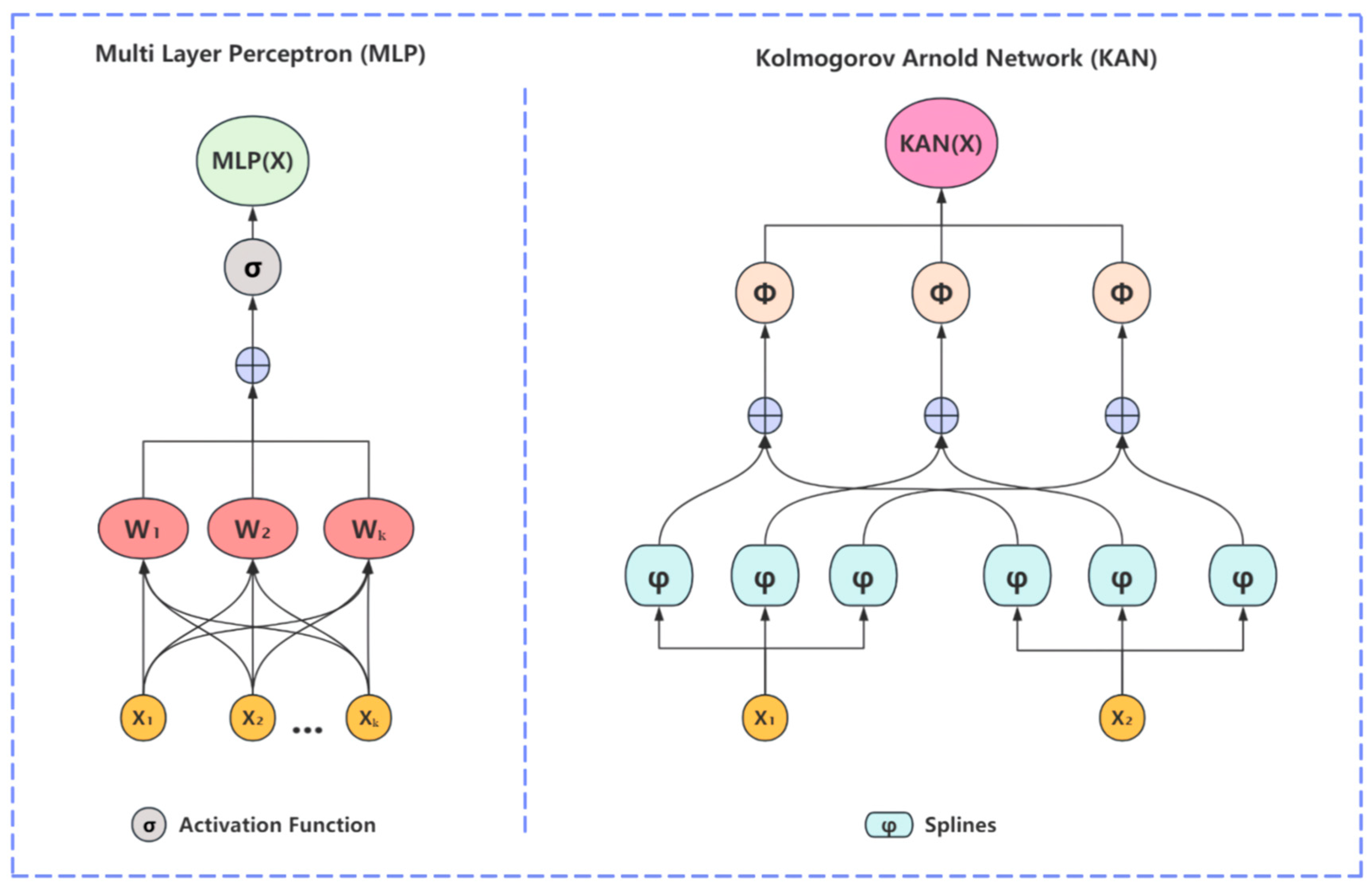
- The Swin Kansformer network model proposed in this paper replaced the traditional MLP layer with the KAN layer, which performs linear transformations of complex functions using nonlinear activation functions to learn and represent complex features. This significantly improved the computational resource consumption, the modeling capability for spatial structures, overfitting risk, local feature capture, and interpretability issues inherent in MLPs.
- (3)
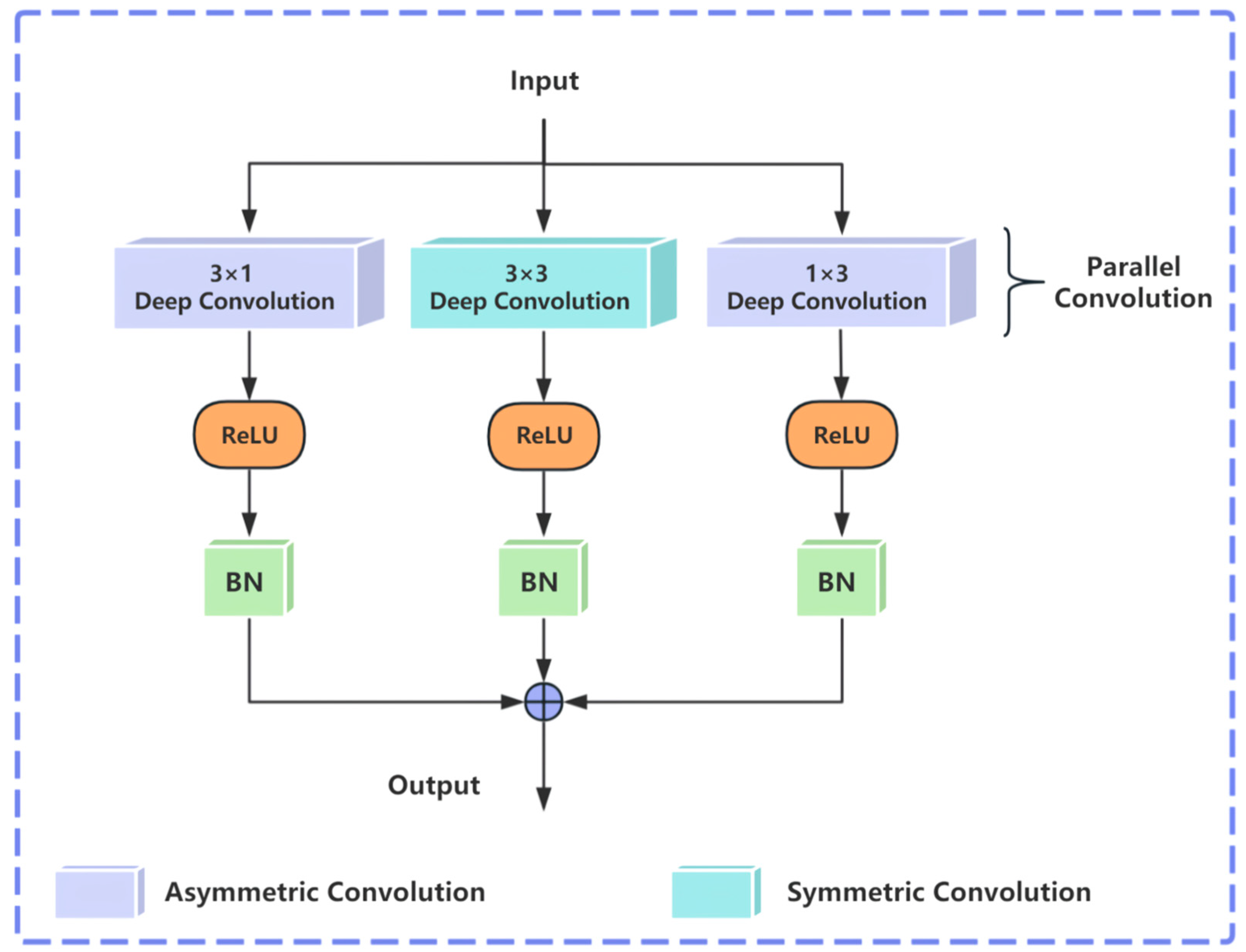
- To enhance the network’s capability in extracting local information, an asymmetric convolution group structure was added to better capture local features while maintaining global feature extraction. This approach fully leveraged both global and local feature information, implementing a global–local feature extraction approach, thereby improving the operational efficiency, computational performance, and ultimately, the classification correctness for remote sensing scene classification assignments.
2. Method
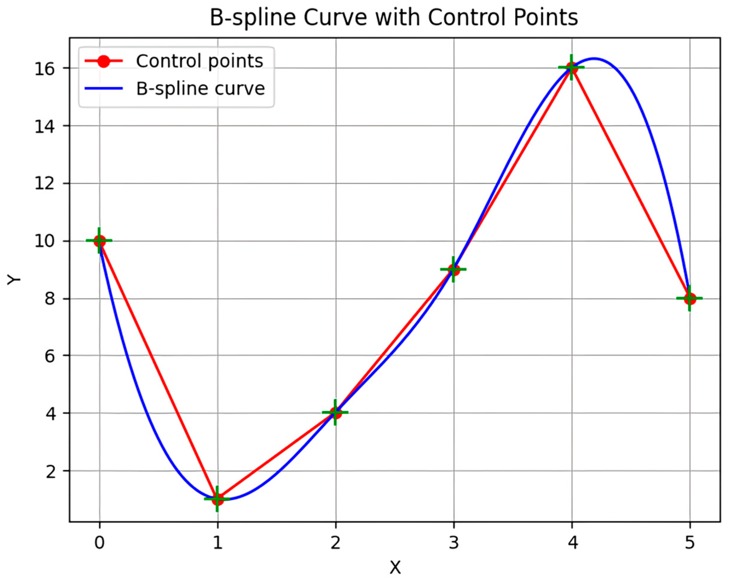
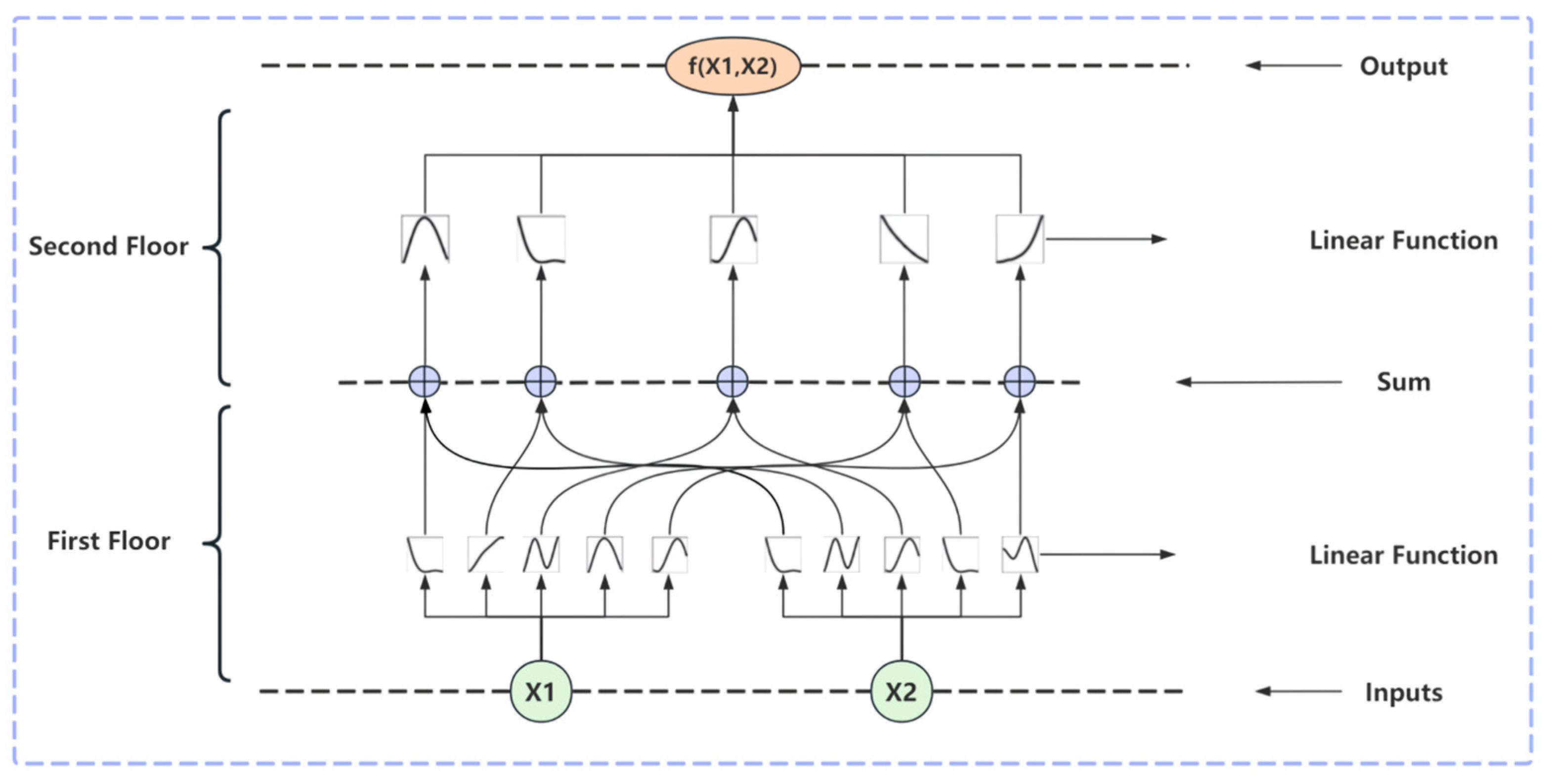
2.1. KAN Theory
- KAN Theoretical Expression
2.2. Swin Kansformer Network
2.2.1. Asymmetric Convolutional Group Module
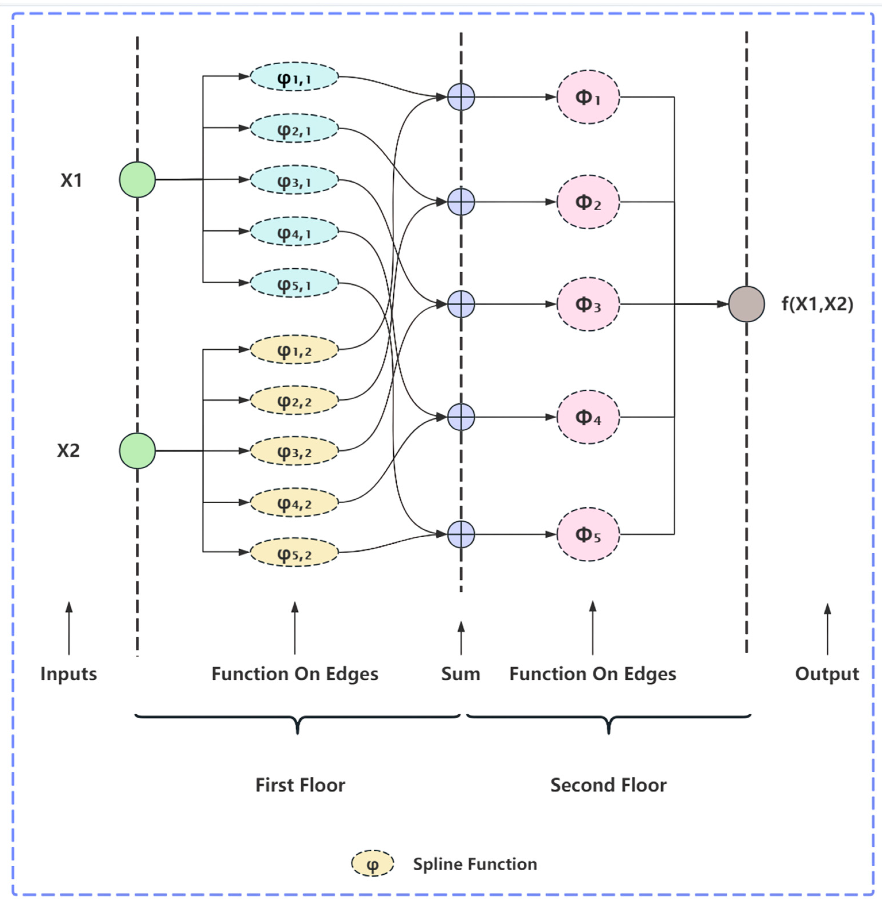
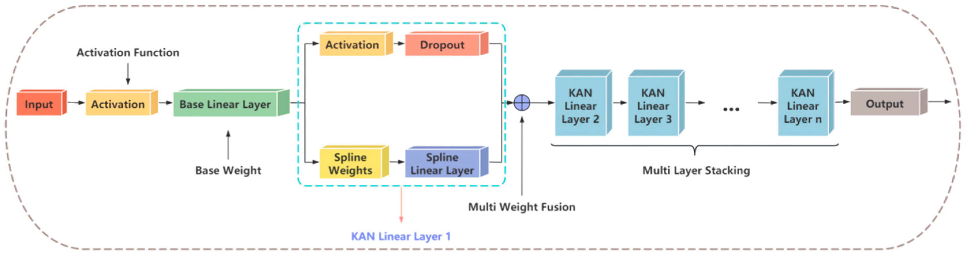
2.2.2. KAN Architecture
2.2.3. KAN Functional Module
KAN Linear
Weight Fusion and Multilayer Stacking
KAN Optimization
3. The Findings of Experiments and Their Analysis
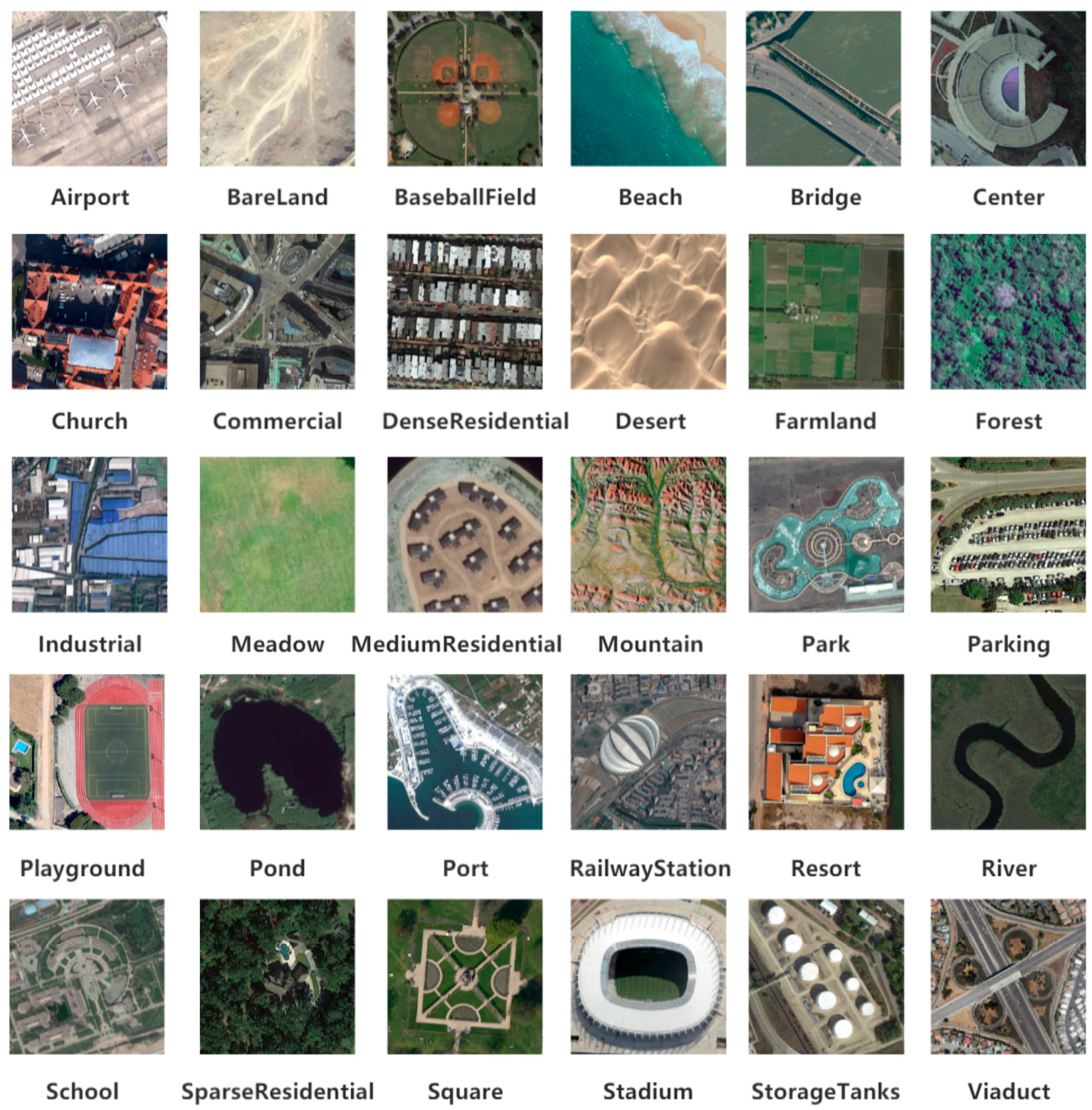
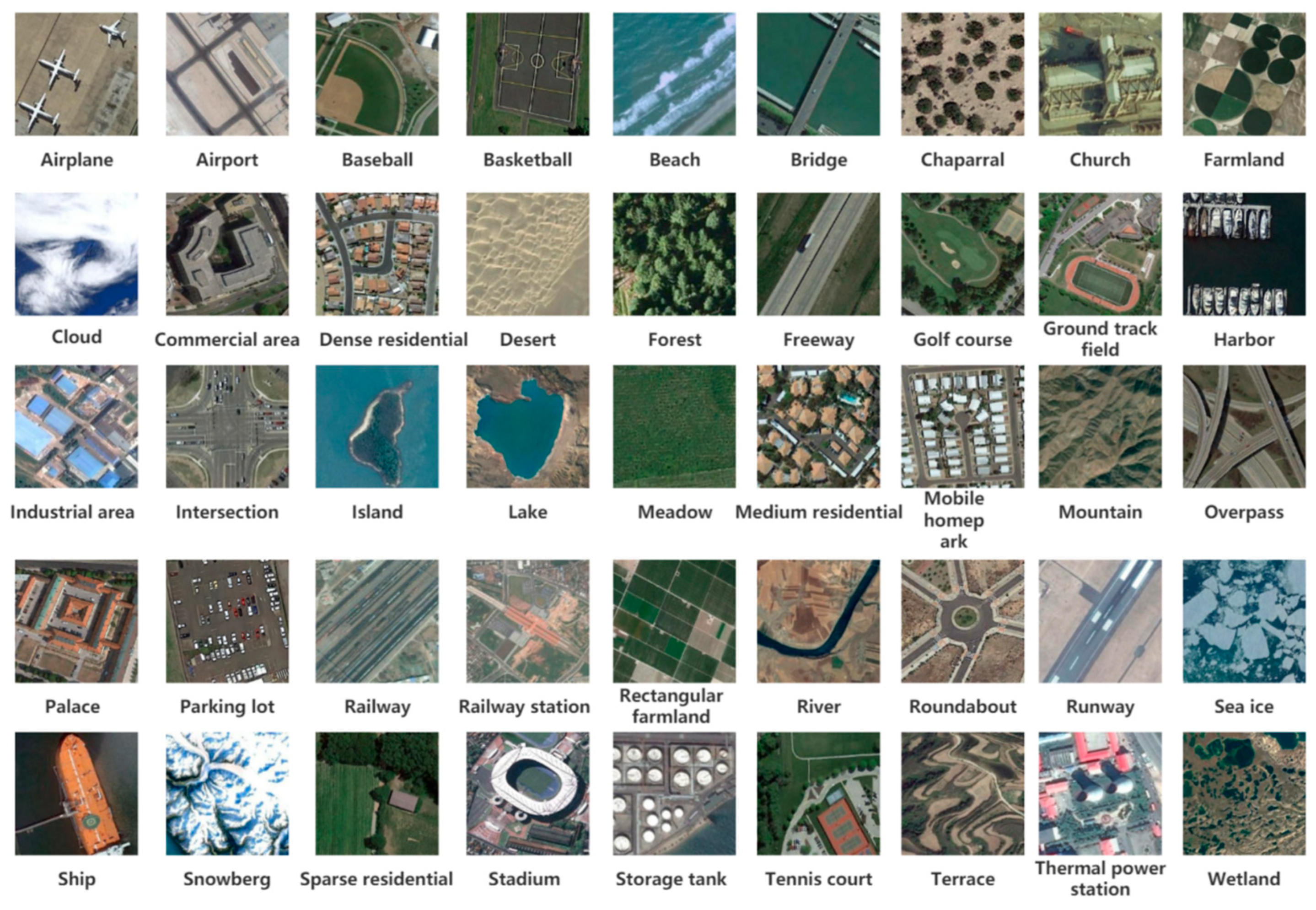
3.1. Description of the Dataset
3.2. Evaluation Metrics
3.3. Experimental Parameter Settings
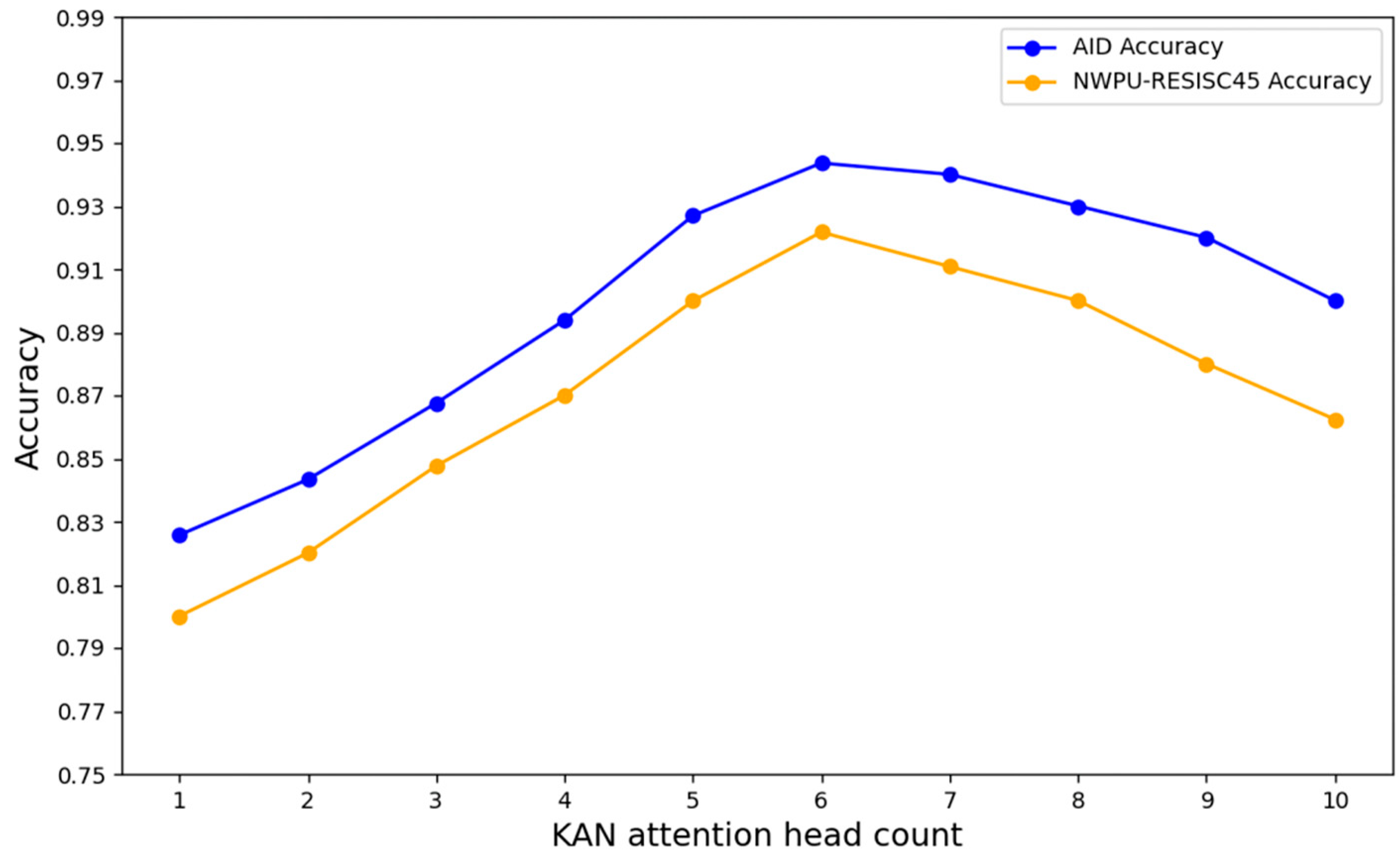
3.4. Hyperparameter Analysis
3.5. Algorithm Performance Comparison
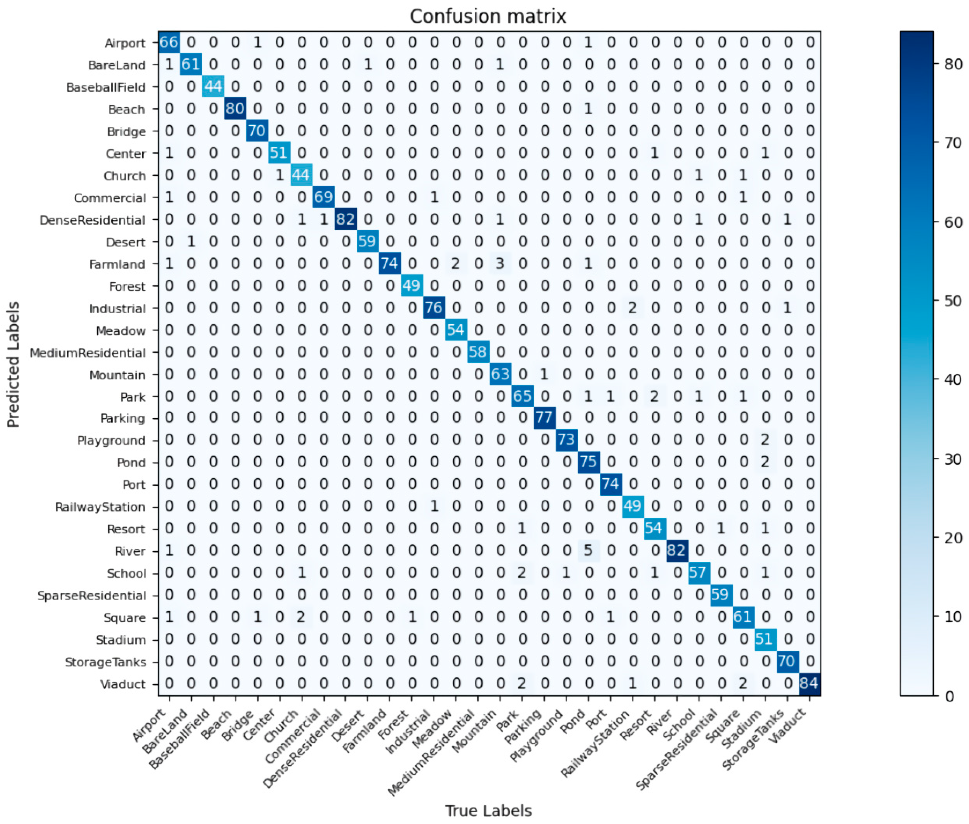
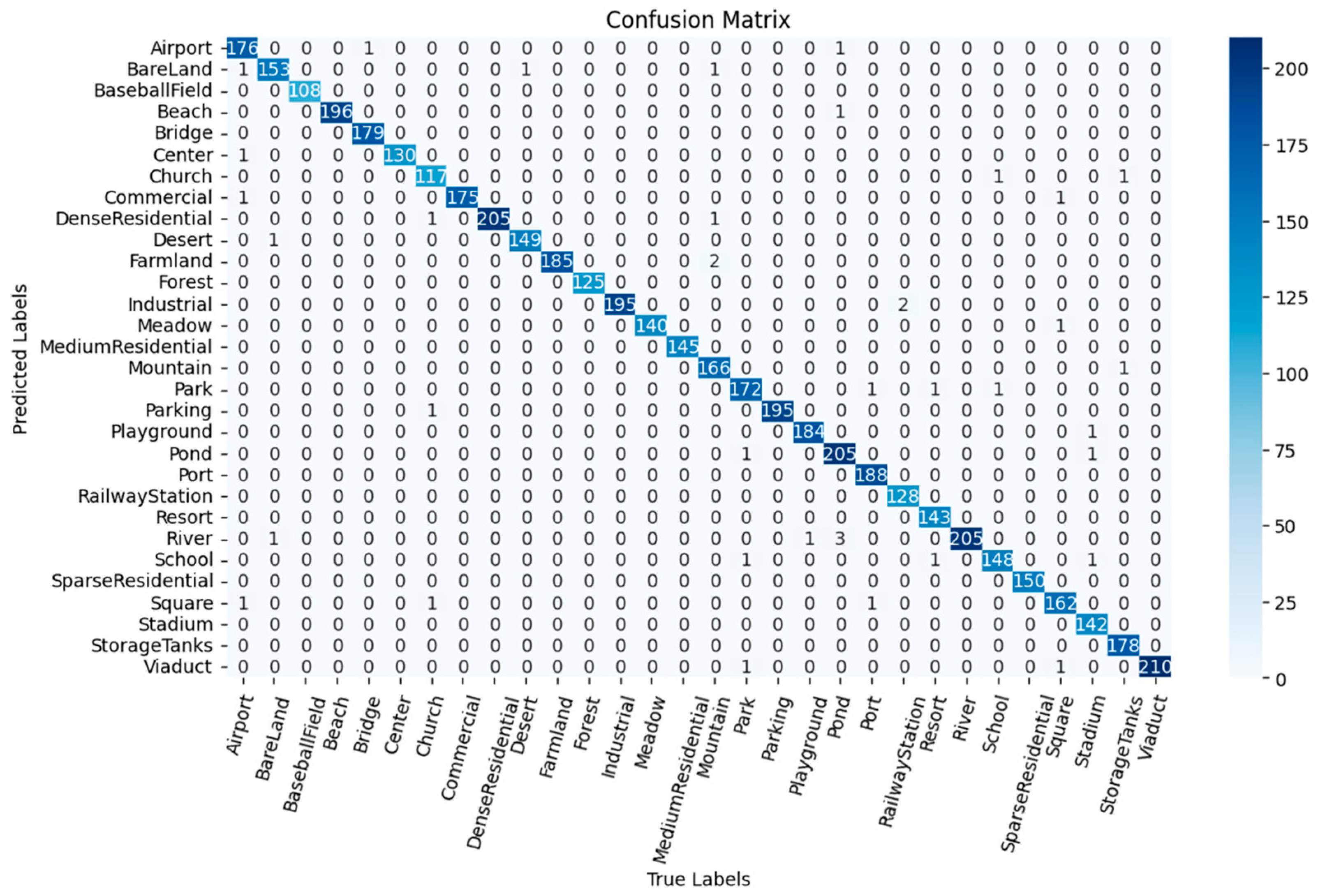
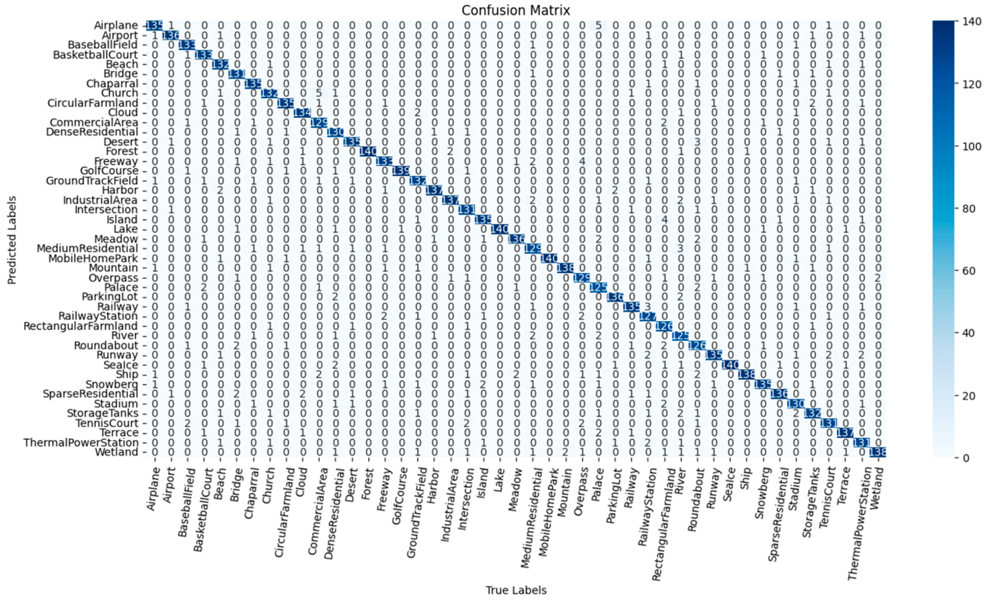
3.6. Confusion Matrix Analysis
3.7. Comparison of Heat Maps
4. Discussion
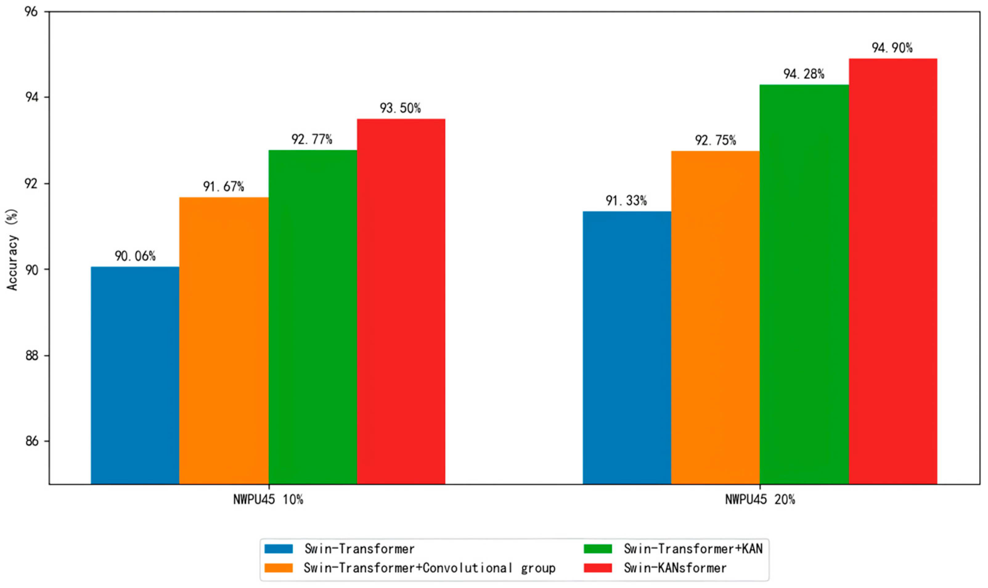
4.1. Ablation Experiment
4.2. Comparative Analysis of KAN Optimization
5. Conclusions
Author Contributions
Funding
Data Availability Statement
Conflicts of Interest
References
- Galleguillos, C.; Belongie, S. Context-based object categorization: A critical survey. Comput. Vis. Image Underst. 2010, 114, 712–722. [Google Scholar] [CrossRef]
- Jalal, A.; Ahmed, A.; Rafique, A.A.; Kim, K. Scene Semantic Recognition Based on Modified Fuzzy C-Mean and Maximum Entropy Using Object-to-Object Relations. IEEE Access 2021, 9, 27758–27772. [Google Scholar] [CrossRef]
- Cheng, G.; Xie, X.; Han, J.; Xia, G.S. Remote sensing image scene classification meets deep learning: Challenges, methods, benchmarks, and opportunities. IEEE J. Sel. Top. Appl. Earth Obs. Remote Sens. 2020, 13, 3735–3756. [Google Scholar] [CrossRef]
- Egenhofer, M.J.; Franzosa, R.D. Point-set topological spatial relations. Int. J. Geogr. Inf. Syst. 1991, 5, 161–174. [Google Scholar]
- Zhu, Q.; Zhong, Y.; Zhao, B.; Xia, G.; Zhang, L. Bag-of-Visual-Words Scene Classifier with Local and Global Features for High Spatial Resolution Remote Sensing Imagery. IEEE Geosci. Remote Sens. Lett. 2016, 13, 747–751. [Google Scholar]
- Zhao, L.J.; Tang, P.; Huo, L.Z. Land-use scene classification using a concentric circle-structured multiscale bag-of-visual-words model. IEEE J. Sel. Top. Appl. Earth Obs. Remote Sens. 2014, 7, 4620–4631. [Google Scholar] [CrossRef]
- Dong, R.; Xu, D.; Jiao, L.; Zhao, J.; An, J. A Fast Deep Perception Network for Remote Sensing Scene Classification. Remote Sens. 2020, 12, 729. [Google Scholar] [CrossRef]
- Chen, J.; Wang, C.; Ma, Z.; Chen, J.; He, D.; Ackland, S. Remote Sensing Scene Classification Based on Convolutional Neural Networks Pre-Trained Using Attention-Guided Sparse Filters. Remote Sens. 2018, 10, 290. [Google Scholar] [CrossRef]
- Cheng, G.; Ma, C.; Zhou, P.; Yao, X.; Han, J. Scene Classification of High Resolution Remote Sensing Images Using Convolutional Neural Networks. In Proceedings of the 2016 IEEE International Geoscience and Remote Sensing Symposium (IGARSS), Beijing, China, 10–15 July 2016; pp. 767–770. [Google Scholar]
- Zhou, W.; Shao, Z.; Cheng, Q. Deep Feature Representations for High-Resolution Remote Sensing Scene Classification. In Proceedings of the 2016 4th International Workshop on Earth Observation and Remote Sensing Applications (EORSA), Guangzhou, China, 4–6 July 2016; pp. 338–342. [Google Scholar]
- Liu, Y.; Liu, Y.; Ding, L. Scene classification based on two-stage deep feature fusion. IEEE Geosci. Remote Sens. Lett. 2017, 15, 183–186. [Google Scholar] [CrossRef]
- Han, X.; Zhong, Y.; Cao, L.; Zhang, L. Pre-trained alexnet architecture with pyramid pooling and supervision for high spatial resolution remote sensing image scene classification. Remote Sens. 2017, 9, 848. [Google Scholar] [CrossRef]
- Muhammad, U.; Wang, W.; Chattha, S.P.; Ali, S. Pre-trained VGGNet architecture for Remote-Sensing Image Scene Classification. In Proceedings of the 2018 24th International Conference on Pattern Recognition, Beijing, China, 20–24 August 2018; pp. 1622–1627. [Google Scholar]
- Tang, P.; Wang, H.; Kwong, S. G-MS2F: GoogLeNet based multi-stage feature fusion of deep CNN for scene recognition. Neurocomputing 2017, 225, 188–197. [Google Scholar] [CrossRef]
- Wang, M.; Zhang, X.; Niu, X.; Wang, F.; Zhang, X. Scene classification of high-resolution remotely sensed image based on ResNet. J. Geovisualization Spat. Anal. 2019, 3, 16. [Google Scholar]
- Dosovitskiy, A.; Beyer, L.; Kolesnikov, A.; Weissenborn, D.; Zhai, X.; Dehghani, M.; Minderer, M.; Heigold, G.; Gelly, S.; Uszkoreit, J. An image is worth 16x16 words: Transformers for image recognition at scale. arXiv 2020, arXiv:2010.11929. [Google Scholar]
- Zheng, F.; Lin, S.; Zhou, W.; Huang, H. A Lightweight Dual-Branch Swin Transformer for Remote Sensing Scene Classification. Remote Sens. 2023, 15, 2865. [Google Scholar] [CrossRef]
- Li, Y.; Yao, T.; Pan, Y.; Mei, T. Contextual Transformer networks for visual recognition. IEEE Trans. Pattern Anal. Mach. Intell. 2023, 45, 1489–1500. [Google Scholar]
- Wang, X.; Duan, L.; Ning, C.; Zhou, H. Relation-attention networks for remote sensing scene classification. IEEE J. Sel. Top. Appl. Earth Obs. Remote Sens. 2021, 15, 422–439. [Google Scholar]
- Liang, J.; Deng, Y.; Zeng, D. A deep neural network combined CNN and GCN for remote sensing scene classification. IEEE J. Sel. Top. Appl. Earth Obs. Remote Sens. 2020, 13, 4325–4338. [Google Scholar]
- Guo, Y.; Ji, J.; Lu, X.; Huo, H.; Fang, T.; Li, D. Global-local attention network for aerial scene classification. IEEE Access 2019, 7, 67200–67212. [Google Scholar]
- Vaswani, A.; Shazeer, N.; Parmar, N.; Uszkoreit, J.; Jones, L.; Gomez, A.N.; Polosukhin, I. Attention is all you need. In Proceedings of the 31st Conference on Advances in Neural Information Processing Systems, Long Beach, CA, USA, 4–9 December 2017; Volume 30. [Google Scholar]
- Haykin, S. Neural networks: A Comprehensive Foundation; Prentice Hall PTR: Hoboken, NJ, USA, 1994. [Google Scholar]
- Cybenko, G. Approximation by superpositions of a sigmoidal function. Math. Control. Signals Syst. 1989, 2, 303–314. [Google Scholar] [CrossRef]
- Hornik, K.; Stinchcombe, M.; White, H. Multilayer feedforward networks are universal approximators. Neural Netw. 1989, 2, 359–366. [Google Scholar]
- Cunningham, H.; Ewart, A.; Riggs, L.; Huben, R.; Sharkey, L. Sparse autoencoders find highly interpretable features in language models. arXiv 2023, arXiv:2309.08600. [Google Scholar]
- Hoefler, T.; Alistarh, D.; Ben-Nun, T.; Dryden, N.; Peste, A. Sparsity in deep learning: Pruning and growth for efficient inference and training in neural networks. J. Mach. Learn. Res. 2021, 22, 1–124. [Google Scholar]
- Liu, Z.; Wang, Y.; Vaidya, S.; Ruehle, F.; Halverson, J.; Soljacĭc, M.; Hou, T.Y.; Tegmark, M. Kan: Kolmogorov-arnold networks. arXiv 2024, arXiv:2404.19756. [Google Scholar]
- Leshno, M.; Lin, V.Y.; Pinkus, A.; Schocken, S. Multilayer feedforward networks with a non-polynomial activation function can approximate any function. Neural Netw. 1993, 6, 861–867. [Google Scholar] [CrossRef]
- Pinkus, A. Approximation theory of the mlp model in neural networks. Acta Numer. 1999, 8, 143–195. [Google Scholar] [CrossRef]
- Kolmogorov, A.N. On the representation of continuous functions of several variables as superpositions of continuous functions of a smaller number of variables. Proc. USSR Acad. Sci. 1956, 108, 179–182. [Google Scholar]
- Kolmogorov, A.N. On the Representation of Continuous Functions of Many Variables by Superposition of Continuous Functions of One Variable and Addition. In Doklady Akademii Nauk; Russian Academy of Sciences: Saint Petersburg, Russia, 1957; Volume 114, pp. 953–956. [Google Scholar]
- Braun, J.; Griebel, M. On a constructive proof of kolmogorov’s superposition theorem. Constr. Approx. 2009, 30, 653–675. [Google Scholar] [CrossRef]
- Schmidt-Hieber, J. The Kolmogorov-Arnold representation theorem revisited. Neural Netw. 2020, 137, 119–126. [Google Scholar] [CrossRef]
- He, J.; Li, L.; Xu, J.; Zheng, C. Relu deep neural networks and linear finite elements. arXiv 2018, arXiv:1807.03973. [Google Scholar]
- He, J.; Xu, J. Deep neural networks and finite elements of any order on arbitrary dimensions. arXiv 2023, arXiv:2312.14276. [Google Scholar]
- Vaca-Rubio, C.J.; Blanco, L.; Pereira, R.; Caus, M. Kolmogorov-arnold networks (kans) for time series analysis. arXiv 2024, arXiv:2405.08790. [Google Scholar]
- Wolf, T.; Kolmogorov-Arnold Networks: The Latest Advance in Neural Networks, Simply Explained. Towards Data Science. 2024. Available online: https://towardsdatascience.com/kolmogorov-arnold-networks-the-latest-advance-in-neural-networks-simply-explained-f083cf994a85/ (accessed on 22 January 2025).
- Bozorgasl, Z.; Chen, H. Wav-kan: Wavelet kolmogorov-arnold networks. arXiv 2024, arXiv:2405.12832. [Google Scholar] [CrossRef]
- LeCun, Y.; Bengio, Y.; Hinton, G. Deep learning. Nature 2015, 521, 436–444. [Google Scholar] [PubMed]
- Udrescu, S.-M.; Tegmark, M. Ai feynman: A physics-inspired method for symbolic regression. Sci. Adv. 2020, 6, eaay2631. [Google Scholar]
- Udrescu, S.-M.; Tan, A.; Feng, J.; Neto, O.; Wu, T.; Tegmark, M. Ai feynman 2.0: Pareto-optimal symbolic regression exploiting graph modularity. Adv. Neural Inf. Process. Syst. 2020, 33, 4860–4871. [Google Scholar]
- Kemker, R.; McClure, M.; Abitino, A.; Hayes, T.; Kanan, C. Measuring Catastrophic Forgetting in Neural Networks. In Proceedings of the AAAI conference on artificial intelligence, New Orleans, LA, USA, 2–7 February 2018; Volume 32. [Google Scholar]
- Ding, X.H.; Guo, Y.C.; Ding, G.G.; Han, J.G. ACNet: Strengthening the Kernel Skeletons for Powerful CNN via Asymmetric Con-volution Blocks. In Proceedings of the 2019 IEEE/CVF International Conference on Computer Vision, Seoul, Korea, 27 October–2 November 2019; IEEE: Piscataway, NJ, USA, 2019; pp. 1911–1920. [Google Scholar] [CrossRef]
- Sprecher, D.A.; Draghici, S. Space-filling curves and kolmogorov superpositionbased neural networks. Neural Netw. 2002, 15, 57. [Google Scholar]
- Köppen, M. On the training of a kolmogorov network. In Proceedings of the Artificial Neural Networks—ICANN 2002: International Conference Madrid, Spain, 28–30 August 2002; Proceedings 12; Springer: Berlin/Heidelberg, Germany, 2002; pp. 474–479. [Google Scholar]
- Lin, J.-N.; Unbehauen, R. On the realization of a kolmogorov network. Neural Comput. 1993, 5, 18. [Google Scholar] [CrossRef]
- Lai, M.-J.; Shen, Z. The kolmogorov superposition theorem can break the curse of dimensionality when approximating high dimensional functions. arXiv 2021, arXiv:2112.09963. [Google Scholar]
- Leni, P.-E.; Fougerolle, Y.D.; Truchetet, F. The kolmogorov spline network for image processing. In Image Processing: Concepts, Methodologies, Tools, and Applications; IGI Global: Hershey, PA, USA, 2013; pp. 54–78. [Google Scholar]
- Fakhoury, D.; Fakhoury, E.; Speleers, H. Exsplinet: An interpretable and expressive spline-based neural network. Neural Netw. 2022, 152, 332–346. [Google Scholar]
- Montanelli, H.; Yang, H. Error bounds for deep relu networks using the kolmogorov–arnold superposition theorem. Neural Netw. 2020, 129, 1–6. [Google Scholar]
- He, J. On the optimal expressive power of relu dnns and its application in approximation with kolmogorov superposition theorem. arXiv 2023, arXiv:2308.05509. [Google Scholar]
- Huang, G.-B.; Zhao, L.; Xing, Y. Towards theory of deep learning on graphs: Optimization landscape and train ability of Kolmogorov-Arnold representation. Neurocomputing 2017, 251, 10–21. [Google Scholar]
- Xing, Y.; Zhao, L.; Huang, G.-B. KolmogorovArnold Representation Based Deep Learning for Time Series Forecasting. In 2018 IEEE Symposium Series on Computational Intelligence (SSCI); IEEE: Piscataway, NJ, USA, 2018; pp. 1483–1490. [Google Scholar]
- Liang, X.; Zhao, L.; Huang, G.-B. Deep Kolmogorov-Arnold representation for learning dynamics. IEEE Access 2018, 6, 49436–49446. [Google Scholar]
- Xia, G.S.; Hu, J.; Hu, F.; Shi, B.; Bai, X.; Zhong, Y.; Lu, X. AID: A benchmark data set for performance evaluation of aerial scene classification. IEEE Trans. Geosci. Remote Sens. 2017, 55, 3965–3981. [Google Scholar] [CrossRef]
- Cheng, G.; Han, J.; Lu, X. Remote sensing image scene classification: Benchmark and state of the art. Proc. IEEE 2017, 105, 1865–1883. [Google Scholar] [CrossRef]
- Ma, A.L.; Yu, N.; Zheng, Z.; Zhong, Y.F.; Zhang, L.P. A supervised progressive growing generative adversarial network for remote sensing image scene classification. IEEE Trans. Geosci. Remote Sens. 2022, 60, 1–18. [Google Scholar] [CrossRef]
- Xu, J.; Zhang, H.; Li, Y. Spectral-Spatial Capsule Networks for Remote Sensing Scene Classification. In IEEE Geoscience and Remote Sensing Letters; IEEE: Piscataway, NJ, USA, 2025. [Google Scholar]
- Liu, Y.; Zhang, X.; Chen, H. Multi-Resolution Fusion Networks for Remote Sensing Scene Classification. In IEEE Transactions on Pattern Analysis and Machine Intelligence; IEEE: Piscataway, NJ, USA, 2025. [Google Scholar]
- Chen, L.; Yang, T.; Zhou, Y. Multi-scale graph convolutional networks for remote sensing scene classification. ISPRS J. Photogramm. Remote Sens. 2024, 62, 4402618. [Google Scholar]
- Wang, J.; Liu, H.; Zhang, W. Efficient Remote Sensing Transformer for Scene Classification. In IEEE International Geoscience and Remote Sensing Symposium (IGARSS); IEEE: Piscataway, NJ, USA, 2024. [Google Scholar]
- Zhao, X.; Wang, Y.; Liu, Z. Efficient Multi-Scale Transformers for Remote Sensing Scene Classification. In IEEE Journal of Selected Topics in Applied Earth Observations and Remote Sensing; IEEE: Piscataway, NJ, USA, 2024. [Google Scholar]
- Lv, P.Y.; Wu, W.J.; Zhong, Y.F.; Du, F.; Zhang, L.P. SCViT: A spatial-channel feature preserving vision transformer for remote sensing image scene classification. IEEE Trans. Geosci. Remote Sens. 2022, 60, 4409512. [Google Scholar] [CrossRef]
- Zhang, Y.; Li, X.; Wang, L. Kernel Attention Network for remote sensing image classification. IEEE Trans. Geosci. Remote Sens. 2023, 61, 1234–1245. [Google Scholar]
- Chen, J.; Liu, H.; Zhang, W. KANet: A Kernel Attention Network for semantic segmentation of remote sensing images. Remote Sens. 2023, 15, 567–580. [Google Scholar]
- Wang, X.; Li, Y. Kernel Attention Network for hyperspectral image classification. IEEE Geosci. Remote Sens. Lett. 2023, 20, 789–793. [Google Scholar]
- Liu, Y.; Zhang, Z. KANet: A Kernel Attention Network for change detection in remote sensing images. Int. J. Remote Sens. 2023, 44, 2345–2360. [Google Scholar]
- Li, H.; Wang, J. Kernel Attention Network for multi-temporal remote sensing image analysis. Remote Sens. Environ. 2023, 285, 113456. [Google Scholar]


| Classification Method | Training Ratio | |
|---|---|---|
| 20% | 50% | |
| SSCapsNet | 92.67 ± 0.43 | 94.01 ± 0.37 |
| MRFN | 92.45 ± 0.44 | 93.89 ± 0.39 |
| MS-GCN | 92.12 ± 0.48 | 93.56 ± 0.41 |
| ERST | 92.89 ± 0.42 | 94.21 ± 0.36 |
| EMST | 92.78 ± 0.42 | 94.12 ± 0.36 |
| EHT | 92.78 ± 0.42 | 94.12 ± 0.36 |
| GAN | 94.51 ± 0.15 | 96.45 ± 0.19 |
| CFDNN | 94.56 ± 0.17 | 96.56 ± 0.24 |
| Combined CNN and GCN | 94.93 ± 0.31 | 96.89 ± 0.10 |
| PVT-V2_B0 | 93.52 ± 0.35 | 96.27 ± 0.14 |
| ViT + LCA | 95.43 ± 0.22 | 96.89 ± 0.41 |
| ViT + PA | 95.31 ± 0.11 | 96.72 ± 0.16 |
| Swin Kansformer | 96.66 ± 0.24 | 97.78 ± 0.22 |
| Classification Method | Training Ratio | |
|---|---|---|
| 10% | 20% | |
| SSCapsNet | 90.34 ± 0.51 | 91.95 ± 0.47 |
| MRFN | 90.12 ± 0.52 | 91.78 ± 0.48 |
| MS-GCN | 89.78 ± 0.53 | 91.45 ± 0.49 |
| ERST | 90.45 ± 0.51 | 92.10 ± 0.46 |
| EMST | 90.45 ± 0.51 | 92.01 ± 0.46 |
| EHT | 90.45 ± 0.51 | 92.01 ± 0.46 |
| GAN | 91.06 ± 0.11 | 93.63 ± 0.12 |
| CFDNN | 91.17 ± 0.13 | 93.83 ± 0.09 |
| Combined CNN and GCN | 90.75 ± 0.21 | 92.87 ± 0.13 |
| PVT-V2_B0 | 89.72 ± 0.16 | 92.95 ± 0.09 |
| ViT + LCA | 92.37 ± 0.20 | 94.63 ± 0.13 |
| ViT + PA | 92.65 ± 0.20 | 94.24 ± 0.16 |
| Swin Kansformer | 93.50 ± 0.18 | 94.90 ± 0.20 |
Disclaimer/Publisher’s Note: The statements, opinions and data contained in all publications are solely those of the individual author(s) and contributor(s) and not of MDPI and/or the editor(s). MDPI and/or the editor(s) disclaim responsibility for any injury to people or property resulting from any ideas, methods, instructions or products referred to in the content. |
© 2025 by the authors. Licensee MDPI, Basel, Switzerland. This article is an open access article distributed under the terms and conditions of the Creative Commons Attribution (CC BY) license (https://creativecommons.org/licenses/by/4.0/).
Share and Cite
An, S.; Zhang, L.; Li, X.; Zhang, G.; Li, P.; Zhao, K.; Ma, H.; Lian, Z. Global–Local Feature Fusion of Swin Kansformer Novel Network for Complex Scene Classification in Remote Sensing Images. Remote Sens. 2025, 17, 1137. https://doi.org/10.3390/rs17071137
An S, Zhang L, Li X, Zhang G, Li P, Zhao K, Ma H, Lian Z. Global–Local Feature Fusion of Swin Kansformer Novel Network for Complex Scene Classification in Remote Sensing Images. Remote Sensing. 2025; 17(7):1137. https://doi.org/10.3390/rs17071137
Chicago/Turabian StyleAn, Shuangxian, Leyi Zhang, Xia Li, Guozhuang Zhang, Peizhe Li, Ke Zhao, Hua Ma, and Zhiyang Lian. 2025. "Global–Local Feature Fusion of Swin Kansformer Novel Network for Complex Scene Classification in Remote Sensing Images" Remote Sensing 17, no. 7: 1137. https://doi.org/10.3390/rs17071137
APA StyleAn, S., Zhang, L., Li, X., Zhang, G., Li, P., Zhao, K., Ma, H., & Lian, Z. (2025). Global–Local Feature Fusion of Swin Kansformer Novel Network for Complex Scene Classification in Remote Sensing Images. Remote Sensing, 17(7), 1137. https://doi.org/10.3390/rs17071137