Article

Extraction, Dynamics, and Driving Factors of Shallow Water Area in Hongze Lake Based on Landsat Imagery

1
College of Ecology and Environment, Nanjing Forestry University, Nanjing 210037, China
2
School of Agriculture Engineering, Jiangsu University, Zhenjiang 212013, China
3
Co-Innovation Center for Sustainable Forestry in Southern China, Nanjing Forestry University, Nanjing 210037, China
*
Author to whom correspondence should be addressed.
Remote Sens. 2025, 17(7), 1128; https://doi.org/10.3390/rs17071128
Submission received: 6 February 2025 / Revised: 19 March 2025 / Accepted: 20 March 2025 / Published: 21 March 2025
(This article belongs to the Special Issue Remote Sensing for Groundwater Hydrology)

Abstract

:
The dynamics of shallow water areas of inland lakes is closely related to the regional ecology and economy. However, it is still a challenge to extract the natural shallow water area for inland lakes using satellite images due to their rapid changes and various human demands. Therefore, we developed a new remote sensing-based method applied in Hongze Lake (one of the largest freshwater lakes in China) to first delineate the lake from the SWIR1 band of Landsat OLI imagery using cold spots in the LISA method, and then distinguish deep and shallow water areas from the G band of Landsat OLI images using hot spots with LISA after masking the lake out, and finally extracting the natural shallow water area by masking aquatic farms out from shallow water areas using farm ridge classification from NDWI images and aggregating points of farm ridges. The results show that (1) the method of this study is efficient in extracting the natural shallow water area with limited effects from aquatic vegetation; (2) water inflow (upstream water supply and precipitation) and the area of aquatic farms, the two dominant factors for the temporal changes in natural shallow water area, contributed 38.3% (positively) and 42.2% (negatively) to the decrease in the natural shallow water area during 2013–2022 in Hongze Lake; (3) the natural shallow water area of Hongze Lake decreased significantly every April as paddy rice farms withdrew a large amount of irrigation water from Hongze Lake. Our research provides a new approach to extract the natural shallow water areas of inland lakes from satellite images and demonstrates that the upstream water supply, precipitation, and agriculture demands are the three main reasons for seasonal and temporal variations in natural shallow water areas for inland lakes.

1. Introduction

Inland lakes, as reservoirs of surface water and storage sites for sedimentary minerals, form an important part of global hydrological, nutrient, and carbon cycles [1,2,3]. Inland lakes have numerous ecological functions, including maintaining ecological balance [4], protecting biodiversity, regulating runoff, replenishing groundwater, improving the ecological environment, and providing habitats for various species. Inland lakes also play important social and economic roles, including irrigating farmland, generating hydroelectric power, supplying drinking water, and providing natural resources [5]. Inland lakes, especially their shallow water areas, are indicators of a changing climate [6] and the dynamics of surrounding ecosystems. The shallow water area of inland lakes is defined by water depths of no more than 3 m and a vegetation cover of less than 30% at low water levels [7]. Shallow water plays an important role in regulating floodwater, climate, agriculture, aquaculture, and the local ecological environment [8].
Significant spatial dynamics (i.e., seasonal and interannual changes) are characteristic of the shallow water areas of inland lakes due to climate change, agriculture and aquaculture, the modification of natural systems, human settlements, and severe weather [9,10]. Therefore, it is necessary to monitor spatial and temporal changes in shallow lake areas frequently and accurately to manage biodiversity, maintain environment safety, and promote economic development [9,10]. Although remote sensing has proven to be able to accurately capture the dynamics of open water [11], it is still a challenge to monitor the temporal and spatial dynamics of natural shallow water areas of inland lakes due to their rapid changes and the demands of human consumption.
Feature extraction from remotely sensed images with various spatial and temporal scales is critical for obtaining the spatial distribution and temporal dynamics of inland lakes [12,13] including their shallow areas. Various land cover classification algorithms, including support vector machines (SVMs) [14], artificial neural networks (ANNs) [15], decision trees (DTs) [16], principal component analysis, linear transformation, and single-band density slicing [13,17], were applied on satellite imagery to extract open water bodies. Those machine learning methods (e.g., SVMs, ANNs, and DTs) have been proven to be effective for open water extraction from satellite images with high accuracy because of their capacity to deal with nonlinear issues and plenty of training rules [18,19]. However, they have high computational complexity, sensitivity to image quality [15,18,20,21,22,23,24], and limitations in dealing with regional differences [25,26,27]. More importantly, the results of open water extraction based on those methods are hard to keep consistent due to their training rules being different for different images. Therefore, the resulting classification lacks spatial and temporal consistency because of the complex optical characteristics of inland lakes. The most popular and efficient method for inland lake extraction is threshold segmentation, which works by calculating a water-related spectral index (e.g., the NDWI) through multi-band or single-band reflectivity [28,29]. Nevertheless, it is challenging to apply the original NDWI algorithm to effectively distinguish water from other built-up areas, prompting improvements in the NDWI by using green and shortwave-infrared (SWIR1) bands to classify water covered areas. Regardless, limitations remain in enabling inland lakes to be distinguished from shadow and dark roads.
More importantly, it is a challenge to select the optimal threshold for inland lake extraction using threshold segmentation. Automatic threshold algorithms (e.g., Otsu threshold slice and trial-and-error) have been used to reduce human intervention [30]. Nevertheless, water extraction via automatic threshold algorithms is affected by the colored dissolved organic matter load, total suspended solids, chlorophyll concentration, the depths and materials of shallow waters, and the variation in observation conditions [30]. Thus, how to precisely identify the optical characteristics of water has become an important direction in remote sensing research to distinguish shallow water areas from similar land features. Research has demonstrated advantages to using different optical properties of visible, shortwave-infrared, and near-infrared bands to distinguish shallow water and inland lakes, particularly with feature extraction methods with spatial and temporal consistency that are not affected by different image conditions. The Spatial autocorrelation Local Index (LISA) is a way to capture spatial clusters (i.e., based on the spatial autocorrelation between a feature and its surroundings) that applies the first law of geography that close objects (in this case, water) are more related to each other than distant objects (i.e., spatial autocorrelation) [31]. The approach fulfills two key criteria: (a) The extent of the significant spatial clustering of similar values around an observation is indicated by its LISA value. (b) The global indicator of spatial association is proportional to the sum of LISA values across all observations [32,33]. LISA has also been shown to be highly accurate in distinguishing land and water in ecological research [33,34,35,36,37]. Therefore, LISA feature extraction that relies on the inherent distinctions in reflective properties between shallow water and inland lakes might have great potential.
Therefore, we applied the LISA method to distinguish shallow and deep-water areas of inland lakes from Landsat OLI images to explore seasonal and annual variations in shallow water areas. Our specific research objectives were (1) to extract inland lakes from Landsat images, distinguishing shallow water from deep-water areas and dividing shallow water areas into natural and aquatic farms, (2) to explore the seasonal and annual variations in natural shallow water areas and aquatic farms, and (3) to evaluate the causes of dynamics in natural shallow water areas and aquatic farms.

2. Materials and Methods
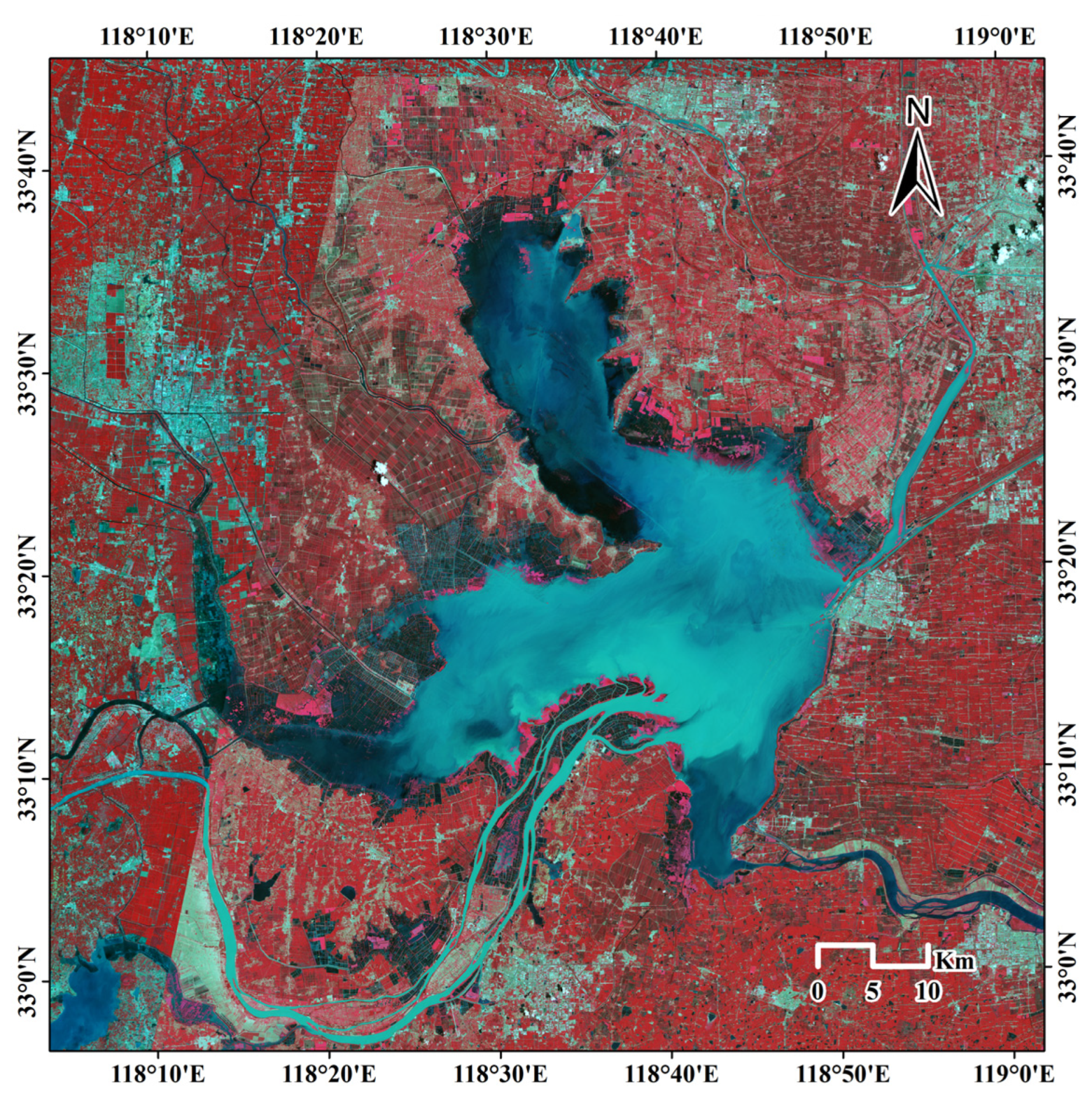
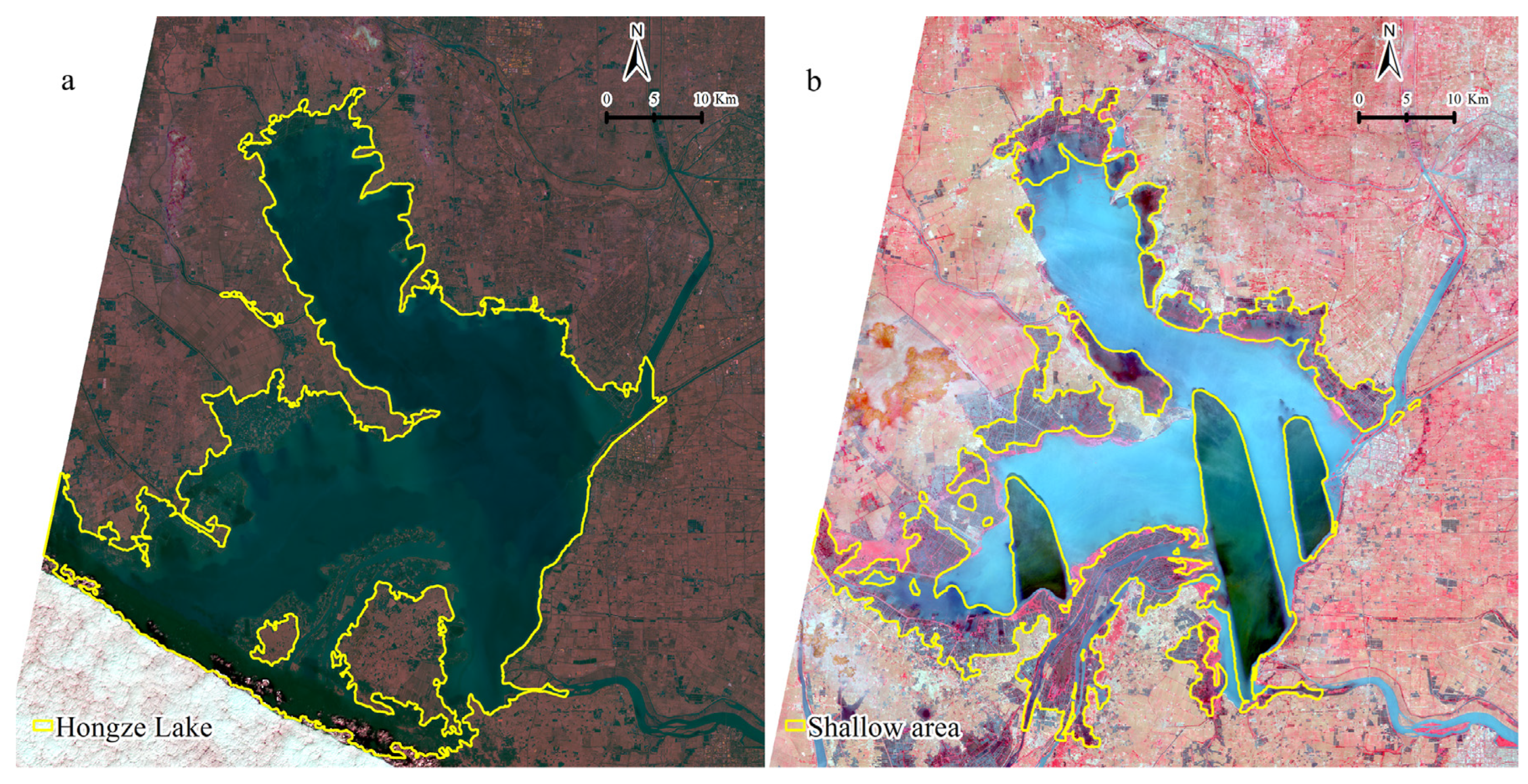
2.1. Study Area

Hongze Lake in the south of the Qinling Mountains, belonging to the Huaihe River Basin, is the fourth largest freshwater lake in China (Figure 1). Because it is located in a transitional zone between the warm temperate zones and the north subtropical zone, Hongze Lake has the properties of a monsoon system with local climate regulation [38]. The mean temperature is 14.8 °C and the annual precipitation average is 926 mm. But in recent years, the water level has fluctuated widely due to climatic characteristics and human disturbances, which have led to apparent changes in the shallow water area of Hongze Lake [39,40]. Hongze Lake encounters various temporal and seasonal changes due to flood disasters, policy changes in aquatic farms, and irrigation demands, which makes it a suitable study area for testing the extraction method of natural shallow water areas.

2.2. Data Collection

2.2.1. Remote Sensing Data

Seventy-two images (spatial resolution: 30 × 30 m) from Landsat 8 and 9 (including 69 Landsat 8 images and 3 Landsat 9 images) acquired during 2013–2022 were downloaded from the USGS website for the extraction of natural shallow area. We used the universal horizontal axis Mercator (UTM) 51N region of the 1984 World Geodesy System (WGS 1984) projection. When obtained from the website, the images (Landsat Collection 2 level 2) were prepossessed by geometric and atmospheric correction. Only cloud-free images were incorporated into the study for shallow water extraction (see details of the Landsat images in Table S1 in Supplementary Material S1, including acquisition dates and sensors).

2.2.2. Meteorological Data and Upstream Water Supply

Precipitation, temperature and upstream water supply are proposed as three factors besides anthropogenic factors for the dynamics of a natural shallow water area. Monthly precipitation and temperature data were obtained from 2013 to 2022 from the NOAA data center that provides global meteorological data, including meteorological observations, meteorological models, and satellite data. Some climate data were also downloaded from Russia’s Weather Data website (https://rp5.ru/; assessed on 1 September 2023) that offers weather data around the world. The data downloaded from these two websites differ and have advantages and disadvantages. The former is more detailed but the database is incomplete, while the latter database is less detailed but is more complete. Therefore, this study downloaded the meteorological data from 2013 to 2020 from the former database, and downloaded the meteorological data from 2021 to 2022 from the latter database for analyses. The data of upstream water supply were obtained from the Huaian Yearbook.

2.2.3. Humanistic Data

Human use data including animal husbandry, fishery output, rural population, and ecological–economic practitioners from 2013 to 2022 were selected from the Huaian statistical yearbook, the Huaian yearbook, and the Huaian Bureau of Statistics (http://tjj.huaian.gov.cn/; assessed on 1 May 2024). Those humanistic data and the extracted area of aquatic farms from Landsat images are used to explore the impact of anthropogenic disturbance on the dynamics of the natural shallow water area in Hongze Lake.

2.3. Methodology

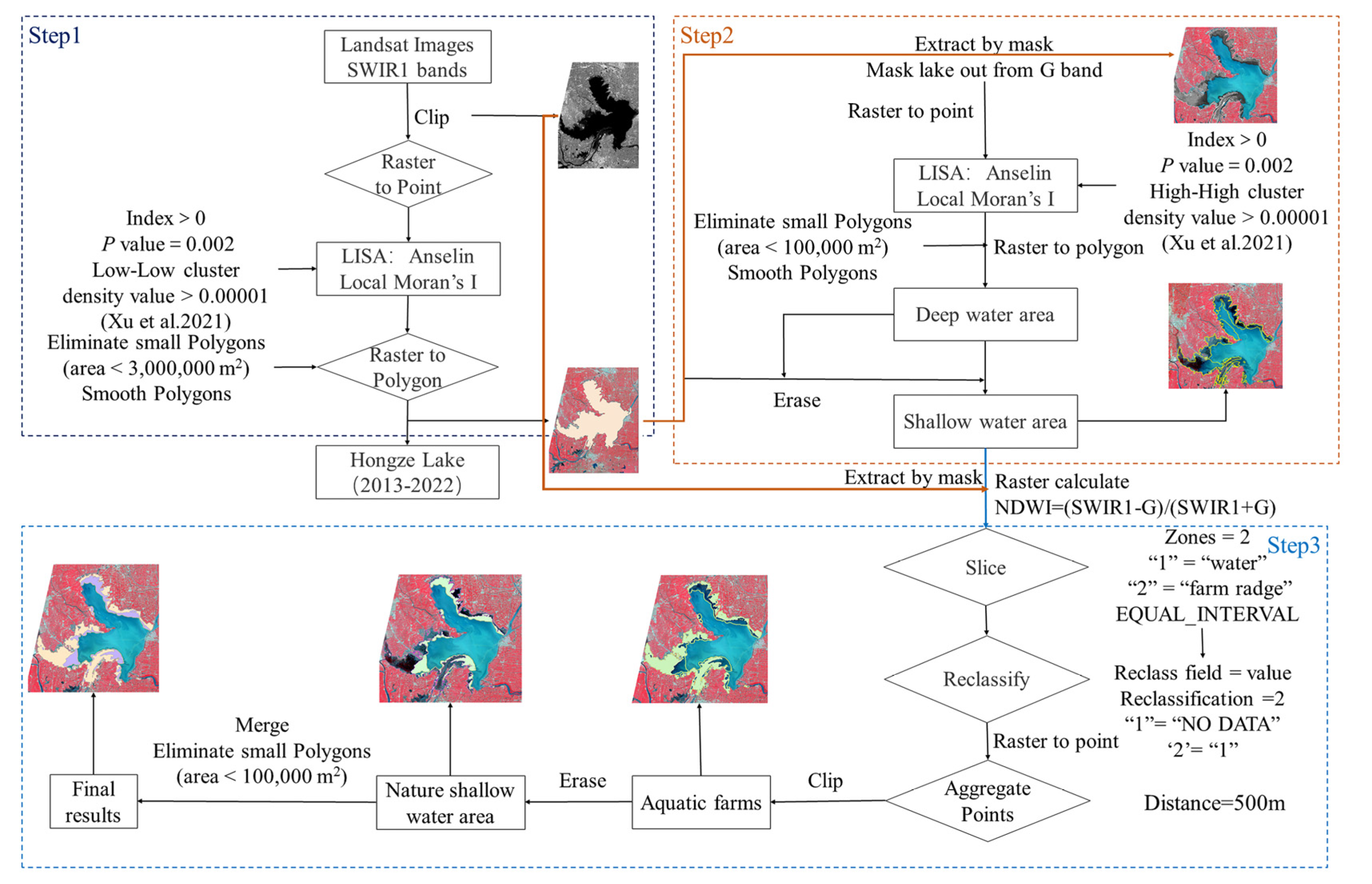
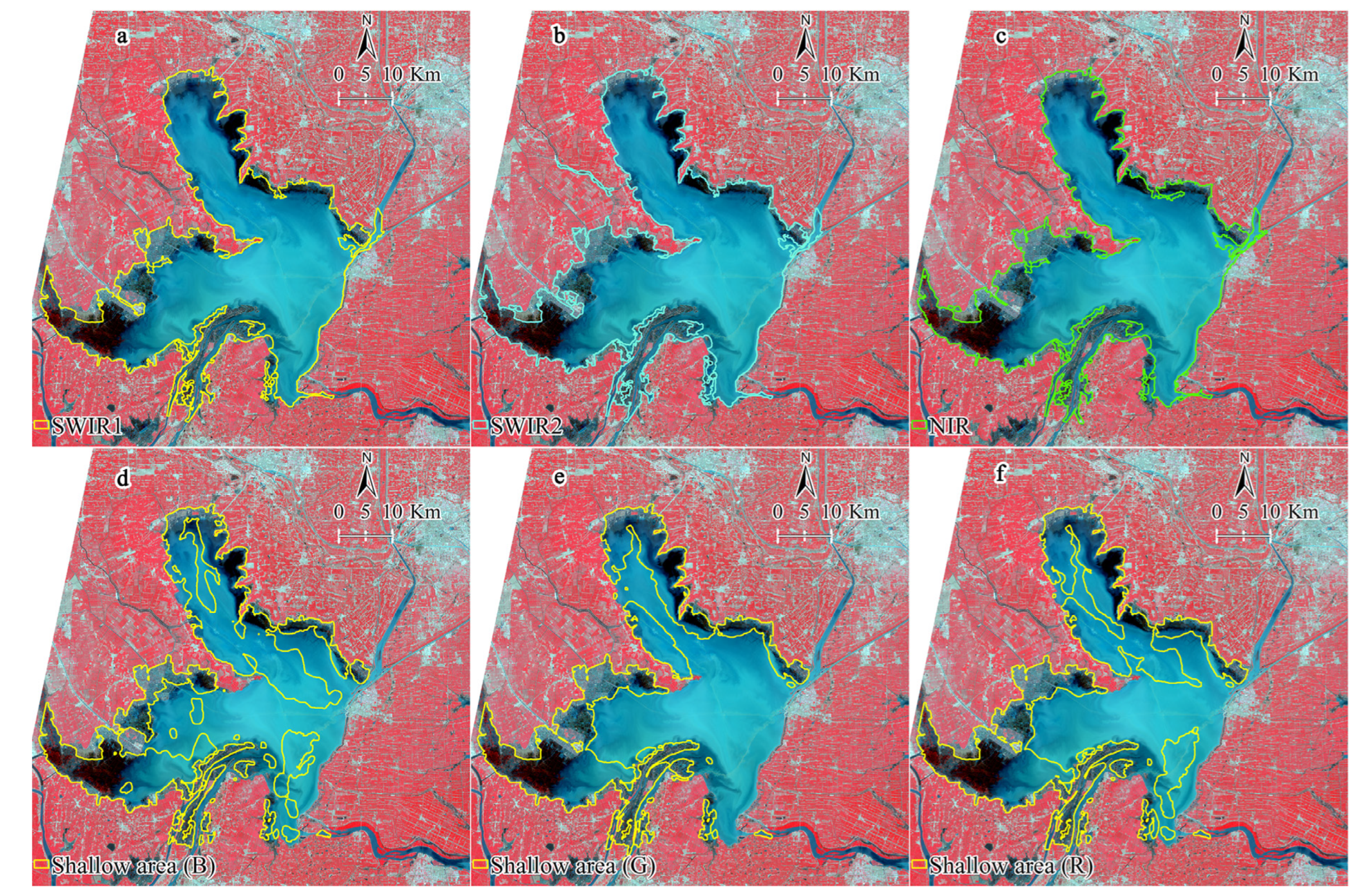
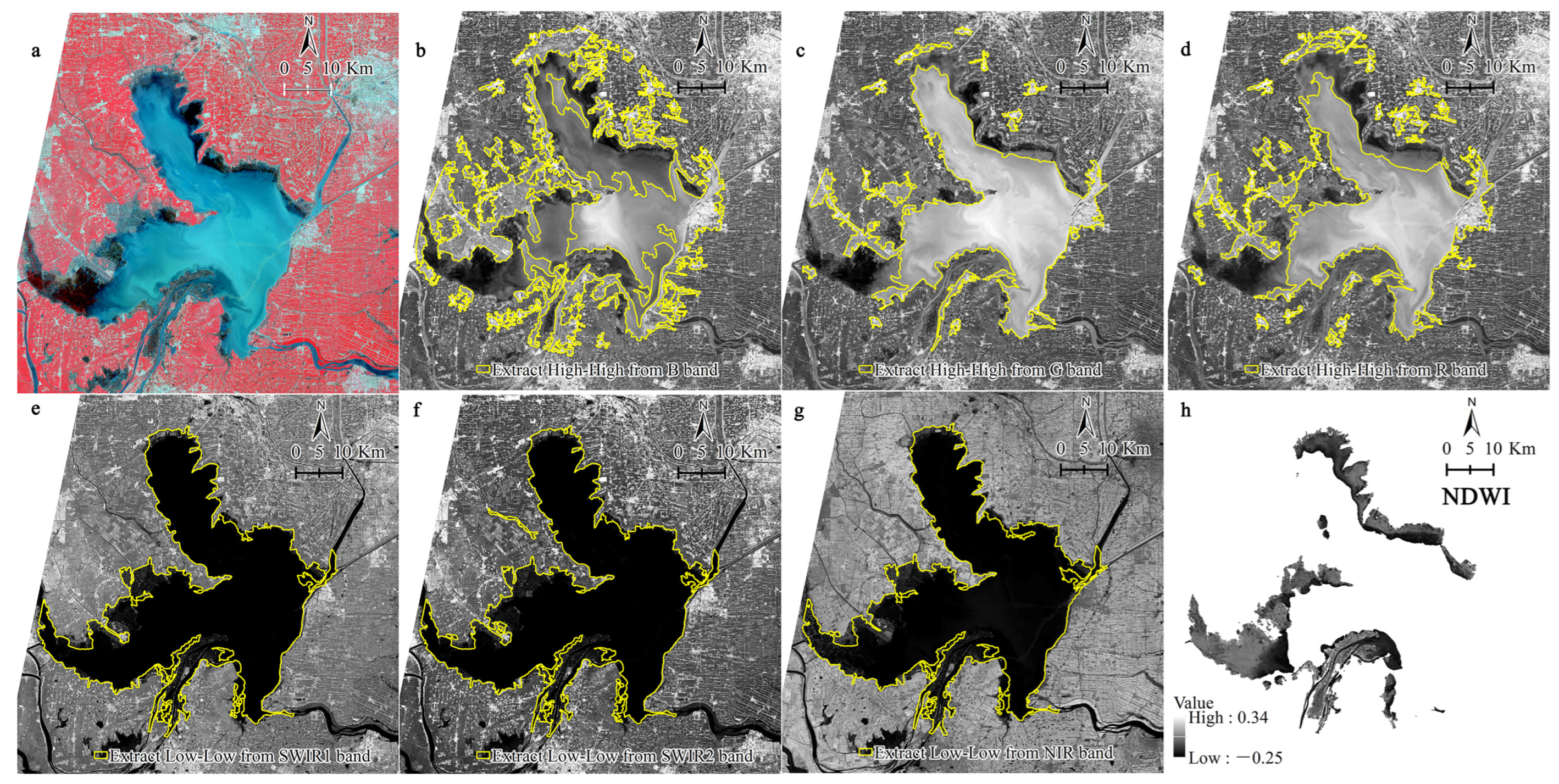
2.3.1. Automatic Extraction of Shallow Area in Hongze Lake

The automatic extraction method for the shallow water area via the LISA identifies spatial clusters based on the concept of spatial autocorrelation between features and their neighboring features (Equation (1); [41,42]). After the preprocessing (images clipped to the Hongze lake area and rastered to points) of the Landsat imagery, the processing steps of this automatic extraction method followed three steps. First, LISA is applied to identify cold spots (i.e., spatial clusters with low values that represent water bodies) from Landsat SWIR1 bands (Figure 2: Step1). The extracted cold spots are the Hongze Lake area because water bodies, including shallow areas, have low reflectance in SWIR1 bands [42]. This is achieved by analyzing preprocessed point-format data of the SWIR1 band using LISA low–low clustering (i.e., the first “low” means a NumPy array with a relatively low value; the second “low” refers to a relatively low value; and all the low values cluster spatially and significance: p value = 0.002 (0.002, the lowest p value of LISA performed in ArcGIS, representing the most significant results of cold spot clusters or hot spot clusters); Figure 2: Step1). Second, the extracted cold spots (Hongze Lake) were used as a mask to extract the corresponding blue (B), green (G) or red (R) bands, and then LISA was applied to extract hot spots from the point-format data of the masked G band. Hot spots were selected in the second step because the deep-water areas of the lake have significantly higher reflectance and a much smoother texture in the G band as well as other visible bands compared to the shallow water area (Figure 2: Step2).
I i = n 1 P i j W i j P j j P j 2 + P i 2
where Pi is the standardized reflectance of one pixel on a single band, Wij is the spatial weight, and n is the number of spatial neighbors, eight spatial neighbors, and Ii is the Local Moran’s index that refers to the spatial association between a given pixel (Pi) and its spatial lag variable j W i j P j which was calculated using the spatial neighbors and their corresponding spatial weigh.
The rest of the lake area, after the deep-water area is delineated (hot spots in the G band) is the shallow water area (Figure 3a). After LISA methods were applied in these two steps, post-processing was performed, including calculating the point density, choosing pixels with a density larger than 0.00001 (number of midpoints per square meter), transforming the chosen pixels into polygons, eliminating small polygons (less than 100,000 m2), and smoothing polygons (Figure 2). The third step divides the extracted shallow water area (Figure 2: Step2) into a natural shallow water area and aquatic farms (Figure 2: Step 3; Figure 3b). Calculating the NDWI index in the shallow water area, masking the aquatic farm ridge out using Slice (i.e., slice method = ‘EQUAL_INTERVAL’; number of out zones = 2; slice the NDWI image into two groups: ‘1’ means water area and ‘2’ means aquatic farm ridge) and reclassifying the sliced image into a farm ridge area only (Reclass field = Value; reclassification = 2), and converting the classification results into point data was the first step. Delineating aquatic farms by applying aggregate points in ArcGIS software 10.8 (aggregation distance: 500 m, which is the optimum distance of this study to aggregate the farm ridge points into aquatic farms) on the point data of aquatic farm ridge followed this. Finally, post-processing, including clipping, erasing, merging, and eliminating polygons in part to merge the extracted aquatic farms into a shallow water area and eliminate some small polygons (area less than 100,000 m2), was completed.

2.3.2. Time Series Analysis of Shallow Water Area

To better identify seasonal and interannual variations in the shallow water area in Hongze Lake, 72 images between 2013 and 2022 were processed to develop a time series dataset. Inevitably, some adverse image factors (haze, cloudy weather, etc.) will affect the Landsat images (16 days of temporal resolution) during the acquisition, which results in missing data in the time series. Therefore, we formed an initial time series dataset using “zoo objects” in the R software (4.3.1) package that identifies missing values. The initial time series dataset aggregates shallow water area data from 2013 to 2022 into monthly time steps using the “aggregate” function in R software (months without data created missing values and multiple values in a month were averaged). Then, we interpolate the missing values using the na.StructTS() (i.e., a seasonal Kalman filter function in the “zoo” package from R software). The seasonal Kalman filter removes missing values in a time series dataset with repeated seasonal variability [43]. After filtering, the final time series dataset with an annual frequency of 12 was created (2013 start, 2022 end). Finally, the seasonal and annual dynamics of the shallow water area were decomposed from the final time series dataset via the Time Series Analysis (TSA) package in “xts” (Extensible Time Series).

2.3.3. Segmented Linear Regression Analysis and Linear Regression

To understand the dynamic changes in the shallow water area in Hongze Lake, we used segmentated linear regression, the widely used method in ecological research [12,44], to analyze the interannual and seasonal changes. In addition, we used the R package (lm), the linear model to assess the influence of driving factors on the shallow water area, calculating Spearman’s r correlation. The significance level of 0.05 (p < 0.05) was selected for all three statistic methods (segmentated linear regression, linear regression, and Spearman’s r correlation).

3. Results

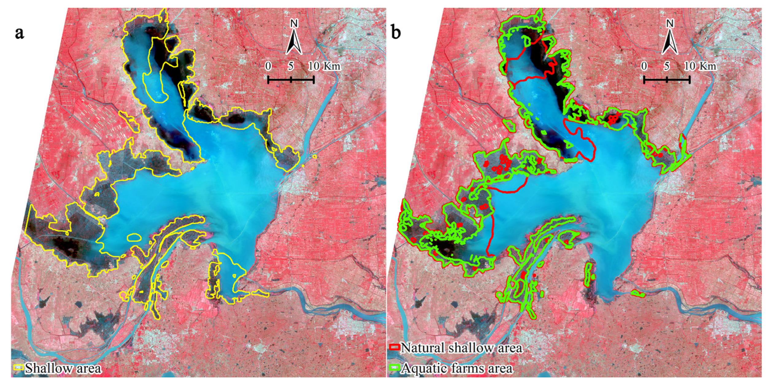
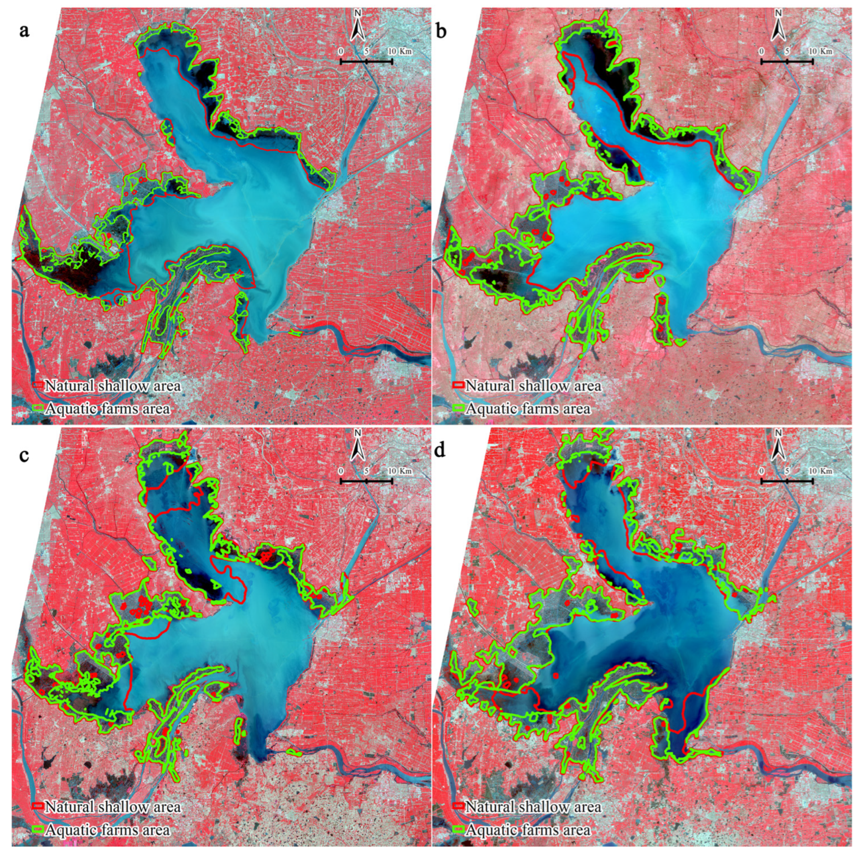
3.1. Extraction of Shallow Water Area

We used SWIR1 bands to extract the Hongze Lake region (Figure 4(a1,b1,c1,d1)), and SWIR1 and G bands were combined to extract the complete shallow water region of Hongze Lake (Figure 4(a2,b2,c2,d2); see extraction results in Supplementary Material S1). One hundred random points in each image were chosen to assess the accuracy for the results of deep and shallow water areas from Landsat OLI images acquired on 7 April 2013, 13 May 2015, and 13 April 2016. The Kappa coefficient of Hongze Lake extraction was 0.881, the overall accuracy was 0.977, while the Kappa coefficient for distinguishing shallow and deep-water regions and overall accuracy was 0.93 and 0.983 (see details in Supplementary Material S2).
Due to the presence of aquatic farms in the extracted shallow water area, it was further divided into a natural shallow water area and aquatic farms (Figure 5). During 2013–2022, the natural shallow water area gradually approached the central area of Hongze Lake, while the aquatic farms gradually expanded the edge of Hongze Lake (Figure 5). We conducted accuracy assessment for natural shallow water areas and aquatic farms from Landsat OLI images acquired on 7 April 2013, 22 February 2017, and 6 April 2019. One hundred random points were chosen to assess the accuracy in each image; the Kappa coefficient of distinguishing natural shallow water and aquatic farms was 0.806 and the overall accuracy was 0.93 (accuracy assessment in Supplementary Material S2).

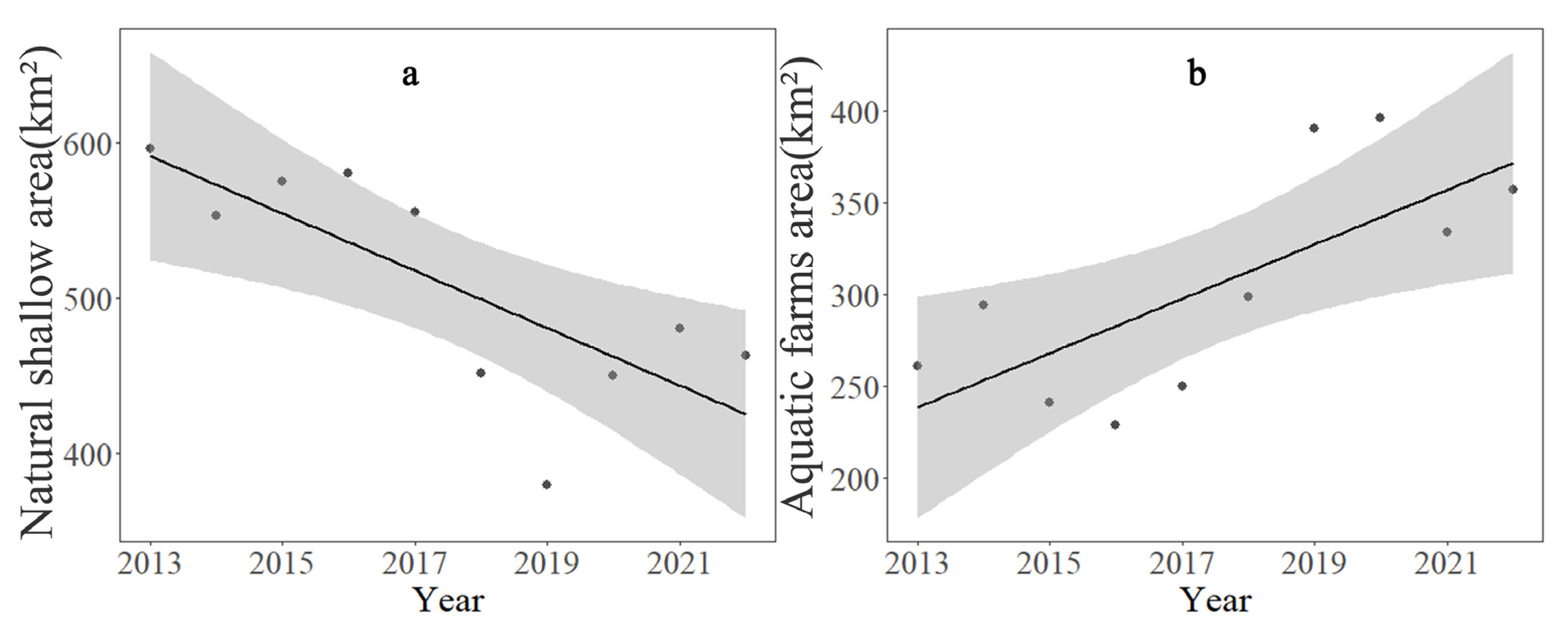
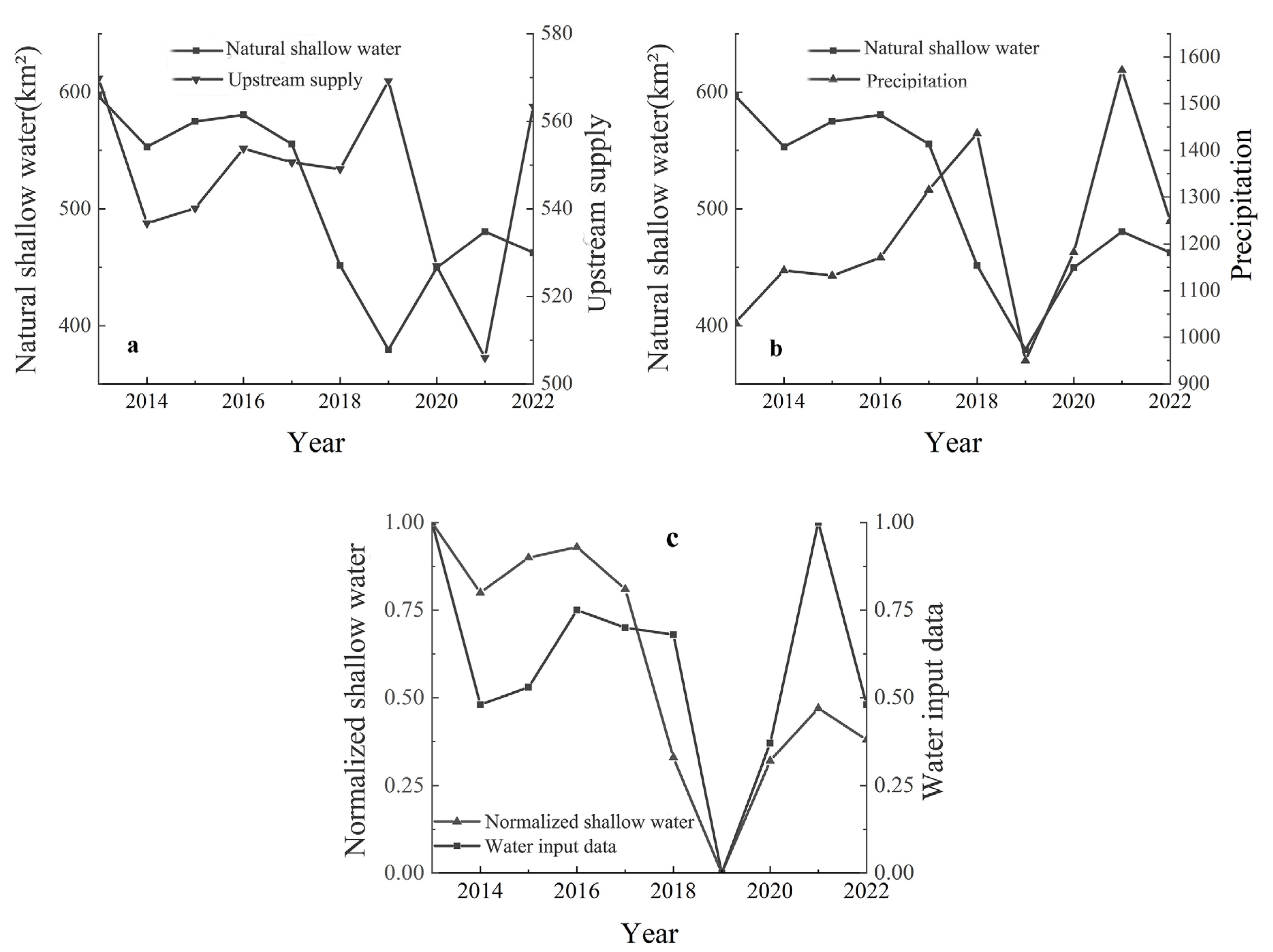
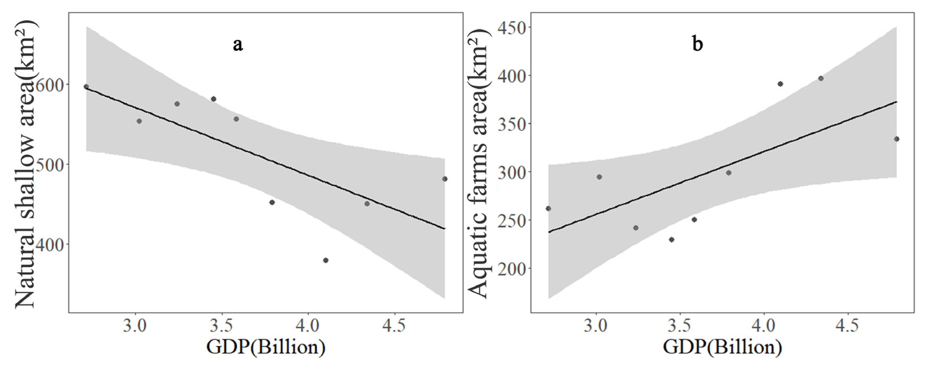
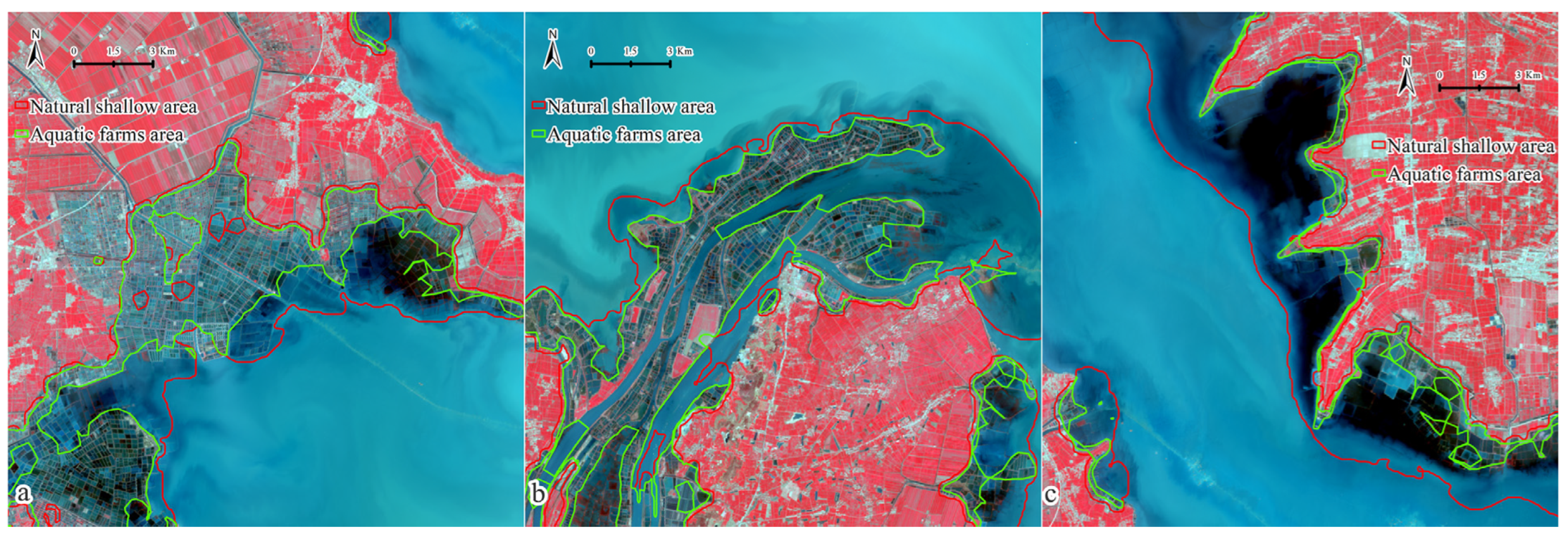
3.2. Temporal Changes in Shallow Water Area and the Driving Factors

From 2013 to 2022, the area of natural shallow water gradually decreased from 596.35 km2 to 462.53 km2 (Figure 6a, p < 0.05), while the anthropogenic shallow water area showed an upward trend from 261.42 km2 to 357.27 km2 (Figure 6b, p < 0.05).
We identified a negative correlation between precipitation and natural shallow water area (r = −0.026, p > 0.05) and a positive correlation between water supply and natural shallow water area (r = 0.093, p > 0.05). The upstream water supply appears to be the principal factor leading to natural shallow water area change before 2018 (Figure 7a), while precipitation is the dominant element for interannual variation in the natural shallow water area after 2018 (Figure 7b). After normalizing the data in natural shallow water area, upstream supply, and precipitation from 2013 to 2022 (i.e., first X = ( x x ¯ ) / s t d ( x ) , then Y = ( X m i n ( X ) ) / ( max X m i n ( X ) ) ), we generated the water input of the natural shallow area by merging the normalized upstream supply (2013–2018) and normalized precipitation (2019–2022). The merged water input is correlated (r = 0.72, p < 0.05) with the natural shallow water area positively in a consistent temporal trend (Figure 7c).
In addition to upstream water and precipitation, the natural shallow water area is affected by economic factors. Regional Gross Domestic Product (GDP; economic output value of agriculture, forestry, fishery, and animal husbandry) is negatively correlated with the natural shallow water area (r = −0.741, p < 0.05; Figure 8a) and positively correlated with aquatic farms area (r = 0.757, p < 0.05; Figure 8b).

3.3. Seasonal Changes in Shallow Water Area and the Driving Factors

There are clear differences in seasonal changes between the natural shallow water area and the area of aquatic farms from April to October (Figure 9). The large drop in natural shallow water areas in April is due to extensive paddy rice irrigation (Figure 9a) and the slight decrease in June is due to flood discharge through opening dam sluice gates to prevent upstream flooding in June and August (peak precipitation in both months; Figure 9a). The seasonal change in aquatic farm areas is relatively stable compared to that of the natural shallow area, with a slight decrease from April to August (Figure 9b).

4. Discussion

4.1. Shallow Water Area Extraction

According to the spectral features of the fresh water in the optical domain (350–2500 mm), the reflectance of water decreases with an increase in wavelength [12]. Water’s reflectance (both shallow and deep regions) in the long wavelength bands (NIR, SWIR1, SWIR2) is much lower than that of other land cover types. Therefore, both shallow and deep-water areas are cold spots in SWIR1, SWIR2, and NIR bands. The methods developed using spatial autocorrelation (LISA) are well suited for detecting cold spots (i.e., low–low clusters) from the three bands (Figure 10a–c).
Cluster extractions from the NIR band were significantly influenced by the presence of aquatic plants (Figure 10c), which caused both the over- or the underestimation of water area in some locations, especially in shallow water. Xu’s [42] results also showed that for open water extraction, the accuracy of NIR was lower than that of SWIR1 and SWIR2 because it was affected by “cumulative noise”. The results from SWIR2 were affected by the cofferdams around Hongze Lake and the fishing and animal husbandry areas [42] in the surrounding area (Figure 10b). Both overestimate the ability to spectrally extract water bodies. In addition, built-up areas and mountain shadows have a large impact on the ability to extract water from the SWIR2 band [45,46]. Among the three bands, SWIR1 performed best for open water extraction including deep and shallow water areas (Figure 10a). Due to the high heterogeneity of Hongze Lake (turbidity, crab farms, and many small tributaries), lake image extraction from the SWIR1 band based on LISA also included small omitted polygons that were eliminated during post-processing (smoothing polygons and eliminating small polygons) [47,48]. Even though the method eliminates unreasonable water extraction results, outcomes are sometimes limited by high water heterogeneity, image quality, or cloud conditions (Figure 11).
Given the regional climate characteristics of Hongze Lake (a temperate subtropical climate transition zone), its hydrological characteristics (over-water lake), human activities, and natural disasters, seasonal floods and flood irrigation resulted in the regular formation of temporary water bodies [30]. These hydrological conditions also affect the accuracy of distinguishing shallow and the deep-water areas. Turbidity, suspended solids, aquatic plants, algae, and various types of organic substance in Hongze Lake all have significant influences on the spectral characteristics of the water [40,49,50]. Image extraction from all three visible bands is also affected by cumulative noise as noted in the NIR [45]. Compared with the B and R bands, better extraction is possible with the G band (Figure 10d–f) because it inhibits vegetation, clearly distinguishing water from plants and algae, and has sensitivity to water transparency.
Water extraction from the G band not only includes deep water but also experiences noise from non-lake regions (Figure 10e). The accurate extraction images of Hongze Lake from the SWIR1 band helps in this case. By clipping the G band using SWIR1 extraction (Figure 12c,e), the noise from non-lake regions is eliminated. Therefore, it accurately distinguished shallow water in Hongze Lake by combining the advantages of the strong water absorption of the SWIR1 and the G bands. This indicates that this method can significantly reduce the influence of hydrological conditions of Hongze Lake to improve the extraction accuracy. Normally, extraction methods in shallow water areas are subject to large differences in water levels between wet and dry years [30] and the particular restrictions of the strong seasonal variability of water surfaces [9,40]. Our approach is based on using different bands from the same image (Figure 12) rather than the seasonal possibilities of water occurrence, which are not influenced by seasonal or temporal variability in the shallow water area. Hongze Lake appears to be larger in the NIR, SWIR1, and SWIR2 bands than in the B, G, and R bands from the same Landsat OLI image (Figure 12). The reflectance is close to zero in the long wavelength bands (NIR, SWIR1, and SWIR2) even for the shallow water area, while the shallow water area does not appear as water bodies in three visible bands because the visible lights penetrate shallow water bodies and reflect the information of the lakebed of the shallow water [51]. The shallow water area of inland lakes is defined by water depths of no more than 3 m and a vegetation cover of less than 30% at low water levels [7]. The extracted shallow water area by the best combination of SWIR1 and G bands based on the LISA method (Figure 12h) depends on the penetration capacity of the G band in Hongze Lake. The accuracy for separating the shallow water area and deep water is high, with a Kappa coefficient of 0.93 and an overall accuracy of 98.3% (Supplementary Material S2). The limitations of this combination for shallow water extraction are the inclusion of aquatic farms, wetlands, and shallow water areas that are not part of the lake, but an adjunct of it (Figure 12h).
The shallow water area is further divided into natural and aquatic farms with the significant difference in spectral characteristics of water and farm ridges. The aquatic farms area is the water area with obvious man-made traces, such as fences, embankments, and other regular construction use; the natural shallow water area is an area with a water depth of less than 3 m and a vegetation coverage of less than 30% except for the aquatic farms area. However, it is not always possible to separate aquatic farms and natural shallow water areas only by classifying farm ridges and water, as aquatic farms include both. Our approach of “aggregate points” for the point format of farm ridges performed well for masking aquatic farms (Figure 13) as it fits polygons around the periphery of the farm ridges instead of distinguishing water regions and farm ridges. However, the abandoned aquatic farms area (i.e., the area which was aquatic farms is recovering as lake are in a process) has been separated as a natural shallow water area because the ridges of the original aquatic farms are not clear any more (Figure 13c). This method for distinguishing natural shallow water and aquatic farms has high accuracy (Kappa coefficient: 0.806; overall accuracy: 90.3%; Supplementary Material S2). The limitation of this distinguishing method is that it is hard to separate aquatic farms and natural shallow water areas when there are no clear fences or ridges of aquatic farms appear in the images, which might cause an overestimation of the natural shallow water area.
However, some aquaculture areas without clear farm ridges and the abandoned aquatic farms with vegetation are misclassified as natural shallow water (Figure 14). The reason for this misclassification is that the aggregation method has certain error sources (aggregation distance and removing small polygons), which will reduce the accuracy of further subdivision in shallow water areas. Previous studies show that the extraction methods for shallow water areas are subject to certain restrictions of the strong seasonal variability of shallow water [9,40], great differences between wet and dry years [30], and the growth status of the aquatic vegetation [52]. Our results find that the aquatic vegetation for abandoned aquatic farms has a significant impact on the extraction of natural shallow water (Figure 14) because the abandoned aquatic farms with aquatic vegetation have no clear farm ridges and the basic step for our method is the classification of farm ridges.
In addition, the source data selected in this study are only Landsat8 and Landsat9 images, and the earlier Landsat5 and Sentinel data are not taken into account, although this can effectively reduce the errors in spatial resolution and radiation resolution caused by different sensors and satellites. However, this will lead to the problem of there being less source data, which will lead to the problem of insufficient quantitative analysis. But in general, The proposed method of this study is effective for extracting the shallow water area of inland lakes and dividing it into natural shallow water areas and aquatic farms. By delineating natural shallow areas and aquatic farms of inland lakes, it helps the lake management focus on the complex and variable areas of inland lakes.

4.2. Dynamics of Shallow Water Area of Hongze Lake and Its Driving Factors

Solitary factors including temperature, precipitation, and upstream water supply are not correlated with changes in the shallow water of Hongze Lake (Table 1). However, the combined effects of upstream supply and precipitation have large effects on natural shallow water area (Figure 9). After data normalization and merging (i.e., the upstream water supply of 2013–2018 and precipitation of 2019–2022), merged water input data are positively correlated with natural shallow water area (Table 1; r = 0.72, p < 0.05). Normally, the upstream water supply is the dominant factor for natural shallow water area when it is larger than 540 billion m3 (Figure 9a). Hongze Lake experienced a severe drought event in 2019 due to low annual precipitation. Thus, the enlarged upstream water supply in this year mitigated the drought effect [53,54]. Nevertheless, the upstream water supply was insufficient to overcome the impact of low precipitation on the natural shallow water area (Figure 9). Indeed, precipitation becomes the dominant factor affecting the lake area only when annual precipitation exceeds 200 mm [55,56]. However, our results show that precipitation became the main water input for Hongze Lake, dominating the change in natural shallow water area, during 2018–2022 (Figure 9) as the relatively low upstream water supply was no longer the dominant factor.
In addition to water input (upstream water supply and precipitation), aquatic farming influences the interannual variation in natural shallow water area (Table 2). Frequent reclamation and aquaculture activities around Hongze Lake are the dominant factors influencing its shallow water area [39,57] and the main reasons for its seasonal changes [8,9,55,58]. Our study indicates that aquatic farming has negative effects on interannual variation in the natural shallow water area; the area of aquatic farms explained 42.2% of the variation in natural shallow water (Table 2).
Although the policies of returning fish and farmland to the lake have been implemented from 2013 to 2022 [58,59], the aquatic farm area continues to increase (Figure 6b). These are dominating factors for the decreasing natural shallow water area during this period. The impact of water input explained relatively little variation in the natural shallow water area (38.3%; Table 2). A mass of major water conservancy facilities are built here, which increases the land use around Hongze Lake, because it is the main water storage area for the South-to-North Water Diversion project [60]. In 2016, the completion of a new round of the Hongze Lake anti-reinforcement project and the Hongze Lake water-level-raising project caused the water level to rise by 0.5 m [39]. These projects that affected the water level would also have caused interannual variation and seasonal changes in the natural shallow water area. Since 2017, Jiangsu Province has continuously promulgated the policy of the “Hongze Lake Regional Comprehensive Protection Plan” and has set up a special committee for Hongze Lake management, which prohibits the abandonment of ships, the unauthorized disposal of silt, land reclamation, and aquaculture. The water required for irrigation has a large impact on the seasonal variation in the natural shallow water. More water is required for the irrigation of spring crops (paddy rice covers about 3100 km2) than for autumn crops (around 3600 km2), resulting in clear seasonal variation in the shallow water area that is consistent with previous research [39,61,62].

5. Conclusions

The method proposed in this study performs well in distinguishing shallow and deep-water areas, and in separating natural shallow areas and aquatic farms. We used the combination of SWIR1 and G band extraction combined with principles of spatial autocorrelation. Natural shallow areas and aquatic farms were separated by classifying farm ridges and aggregating points. Errors tended to be caused by aquatic vegetation. The natural shallow area consistently decreased from 2013 to 2022, driven by water input (upstream water supply and precipitation) and the area of aquatic farms. Aquatic farm area negatively affects and contributes 42.2% to the interannual variation in the natural shallow water area, while water input explains 38.3% of the positive variation in natural shallow water area. We also found that upstream water supply is the dominant factor when it exceeds 540 billion m3, while precipitation becomes the dominant factor for the natural shallow water area when the upstream water supply is relatively low. Finally, the natural shallow water area drops significantly each April due to demands for paddy rice irrigation.

Supplementary Materials

The following supporting information can be downloaded at: https://www.mdpi.com/article/10.3390/rs17071128/s1, Supplementary S1: all the extraction results; Supplementary S2: accuracy assessment.

Author Contributions

Conceptualization, N.L. and D.X.; methodology, N.L. and D.X.; validation, N.L., J.H. and N.N.; formal analysis, N.L. and D.X.; investigation, N.L., J.H. and N.N.; resources, D.X. and Z.L.; writing—original draft preparation, N.L.; writing—review and editing, D.X.; visualization, N.L., J.H. and N.N.; supervision, D.X.; project administration, Z.L.; funding acquisition, N.L. and D.X. All authors have read and agreed to the published version of the manuscript.

Funding

This research was funded by the National Natural Science Foundation of China (41901361), the China Postdoctoral Science Foundation (2023M741430) and the Postgraduate Research & Practice Innovation Program of Jiangsu Province.

Data Availability Statement

The original contributions presented in this study are included in the article/Supplementary Materials. Further inquiries can be directed to the corresponding author.

Acknowledgments

The authors would like to acknowledge John Wilmshurst for English proofreading.

Conflicts of Interest

The authors declare no conflicts of interest.

References

  1. Sun, M.; Zhang, L.; Yang, R.; Li, X.; Zhao, J.; Liu, Q. Water resource dynamics and protection strategies for inland lakes: A case study of hongjiannao lake. J. Environ. Manag. 2024, 355, 120462. [Google Scholar] [CrossRef] [PubMed]
  2. Yu, H.; Tu, Z.; Yu, G.; Xu, L.; Wang, H.; Yang, Y. Shrinkage and protection of inland lakes on the regional scale: A case study of hubei province, china. Reg. Environ. Change 2020, 20, 4. [Google Scholar] [CrossRef]
  3. Tranvik, L.J.; Cole, J.J.; Prairie, Y.T. The study of carbon in inland waters—From isolated ecosystems to players in the global carbon cycle. Limnol. Oceanogr. Lett. 2018, 3, 41–48. [Google Scholar] [CrossRef]
  4. Bai, S.; Gao, J.; Pu, Y.; Zhi, D.; Yao, J. Exploring the relationship between hydroclimate and lake area in source area of the yellow river: Implications for the paleoclimate studies. Atmosphere 2023, 14, 897. [Google Scholar] [CrossRef]
  5. Liu, X.; Shi, Z.; Huang, G.; Bo, Y.; Chen, G. Time series remote sensing data-based identification of the dominant factor for inland lake surface area change: Anthropogenic activities or natural events? Remote Sens. 2020, 12, 612. [Google Scholar] [CrossRef]
  6. Zhang, G.Q.; Duan, S.Q. Lakes as sentinels of climate change on the tibetan plateau. All Earth 2021, 33, 161–165. [Google Scholar] [CrossRef]
  7. Nõges, T. Relationships between morphometry, geographic location and water quality parameters of european lakes. Hydrobiologia 2009, 633, 33–43. [Google Scholar] [CrossRef]
  8. Liu, B.J.; Xia, J.; Zhu, F.L.; Quan, J.; Wang, H. Response of hydrodynamics and water-quality conditions to climate change in a shallow lake. Water Resour. Manag. 2021, 35, 4961–4976. [Google Scholar] [CrossRef]
  9. Guo, M.; Ma, S.; Wang, L.J.; Lin, C. Impacts of future climate change and different management scenarios on water-related ecosystem services: A case study in the jianghuai ecological economic zone, china. Ecol. Indic. 2021, 127, 107732. [Google Scholar] [CrossRef]
  10. Chapman, M.G.; Huang, L.; Han, Y.; Zhou, Y.; Gutscher, H.; Bi, J. How do the chinese perceive ecological risk in freshwater lakes? PLoS ONE 2013, 8, e62486. [Google Scholar]
  11. Xu, D.D.; Geng, Q.H.; Jin, C.S.; Xu, Z.K.; Xu, X. Tree line identification and dynamics under climate change in wuyishan national park based on landsat images. Remote Sens. 2020, 12, 2890. [Google Scholar] [CrossRef]
  12. Chen, Y.; Fan, R.; Yang, X.; Wang, J.; Latif, A. Extraction of urban water bodies from high-resolution remote-sensing imagery using deep learning. Water 2018, 10, 585. [Google Scholar] [CrossRef]
  13. Ghosh, M.K.; Kumar, L.; Roy, C. Monitoring the coastline change of hatiya island in bangladesh using remote sensing techniques. Isprs J. Photogramm. Remote Sens. 2015, 101, 137–144. [Google Scholar] [CrossRef]
  14. Meng, X.R.; Zhang, S.Q.; Zang, S.Y. Lake wetland classification based on an svm-cnn composite classifier and high-resolution images using wudalianchi as an example. J. Coast. Res. 2019, 93, 153–162. [Google Scholar] [CrossRef]
  15. Lezine, E.M.D.; Kyzivat, E.D.; Smith, L.C. Super-resolution surface water mapping on the canadian shield using planet cubesat images and a generative adversarial network. Can. J. Remote Sens. 2021, 47, 261–275. [Google Scholar] [CrossRef]
  16. Hin, L.Z.; Othman, Z. Lake chini water level prediction model using classification techniques. In Proceedings of the 6th International Conference on Computational Science and Technology (ICCST), Spatial Explorer, Kota Kinabalu, Malaysia, 29–30 August 2019; Springer: Singapore, 2020; pp. 215–226. [Google Scholar]
  17. Liu, Z.F.; Yao, Z.J.; Wang, R. Assessing methods of identifying open water bodies using landsat 8 oli imagery. Environ. Earth Sci. 2016, 75, 873. [Google Scholar] [CrossRef]
  18. Li, W.; Fu, H.; Yu, L.; Cracknell, A. Deep learning based oil palm tree detection and counting for high-resolution remote sensing images. Remote Sens. 2016, 9, 22. [Google Scholar] [CrossRef]
  19. Isikdogan, F.; Bovik, A.C.; Passalacqua, P. Surface water mapping by deep learning. IEEE J. Sel. Top. Appl. Earth Obs. Remote Sens. 2017, 10, 4909–4918. [Google Scholar] [CrossRef]
  20. Zhu, S.; Lu, H.; Ptak, M.; Dai, J.; Ji, Q. Lake water-level fluctuation forecasting using machine learning models: A systematic review. Environ. Sci. Pollut. Res. 2020, 27, 44807–44819. [Google Scholar] [CrossRef]
  21. Sannasi Chakravarthy, S.R.; Bharanidharan, N.; Rajaguru, H. A systematic review on machine learning algorithms used for forecasting lake-water level fluctuations. Concurr. Comput. Pract. Exp. 2022, 34, e7231. [Google Scholar] [CrossRef]
  22. Nagaraj, R.; Kumar, L.S. Extraction of surface water bodies using optical remote sensing images: A review. Earth Sci. Inform. 2024, 17, 893–956. [Google Scholar] [CrossRef]
  23. Jiang, W.; He, G.; Long, T.; Ni, Y.; Liu, H.; Peng, Y.; Lv, K.; Wang, G. Multilayer perceptron neural network for surface water extraction in landsat 8 oli satellite images. Remote Sens. 2018, 10, 755. [Google Scholar] [CrossRef]
  24. Liao, A.; Chen, L.; Chen, J.; He, C.; Cao, X.; Chen, J.; Peng, S.; Sun, F.; Gong, P. High-resolution remote sensing mapping of global land water. Sci. China Earth Sci. 2014, 57, 2305–2316. [Google Scholar] [CrossRef]
  25. Shen, M.; Zhang, F.; Wu, C.Y. Flood inundation extraction based on decision-level data fusion: A case in peru. ISPRS Ann. Photogramm. Remote Sens. Spat. Inf. Sci. 2022, X-3/W1-2022, 133–140. [Google Scholar] [CrossRef]
  26. Du, J.K.; Feng, X.Z.; Wang, Z.L.; Huang, Y.S.; Ramadan, E. The methods of extracting water information from spot image. Chin. Geogr. Sci. 2002, 12, 68–72. [Google Scholar] [CrossRef]
  27. Zhang, H.; Li, Q.; Liu, J.; Du, X.; Dong, T.; McNairn, H.; Champagne, C.; Liu, M.; Shang, J. Object-based crop classification using multi-temporal spot-5 imagery and textural features with a random forest classifier. Geocarto Int. 2017, 33, 1017–1035. [Google Scholar] [CrossRef]
  28. Xu, H.Q. Modification of normalised difference water index (ndwi) to enhance open water features in remotely sensed imagery. Int. J. Remote Sens. 2006, 27, 3025–3033. [Google Scholar] [CrossRef]
  29. Guo, Q.D.; Pu, R.L.; Zhang, B.; Gao, L.R. A comparative study of coastline changes at tampa bay and xiangshan harbor during the last 30 years. In Proceedings of the 36th IEEE International Geoscience and Remote Sensing Symposium (IGARSS), Beijing, China, 10–15 July 2016; pp. 5185–5188. [Google Scholar]
  30. Pekel, J.-F.; Cottam, A.; Gorelick, N.; Belward, A.S. High-resolution mapping of global surface water and its long-term changes. Nature 2016, 540, 418–422. [Google Scholar] [CrossRef]
  31. Bi, S.; Li, Y.; Xu, J.; Liu, G.; Song, K.; Mu, M.; Lyu, H.; Miao, S.; Xu, J. Optical classification of inland waters based on an improved fuzzy c-means method. Opt. Express 2019, 27, 34838–34856. [Google Scholar] [CrossRef]
  32. Anselin, L. Local indicators of spatial association—Lisa. Geogr. Anal. 2010, 27, 93–115. [Google Scholar] [CrossRef]
  33. Kowe, P.; Mutanga, O.; Odindi, J.; Dube, T. Exploring the spatial patterns of vegetation fragmentation using local spatial autocorrelation indices. J. Appl. Remote Sens. 2019, 13, 024523. [Google Scholar] [CrossRef]
  34. Bioresita, F.; Puissant, A.; Stumpf, A.; Malet, J.-P. A method for automatic and rapid mapping of water surfaces from sentinel-1 imagery. Remote Sens. 2018, 10, 217. [Google Scholar] [CrossRef]
  35. Wang, L.; Shi, C.; Diao, C.; Ji, W.; Yin, D. A survey of methods incorporating spatial information in image classification and spectral unmixing. Int. J. Remote Sens. 2016, 37, 3870–3910. [Google Scholar] [CrossRef]
  36. Xu, D.D.; Zhang, D.; Shi, D.; Luan, Z.Q. Automatic extraction of open water using imagery of landsat series. Water 2020, 12, 1928. [Google Scholar] [CrossRef]
  37. Zhang, X.H.; Guo, Z.Y.; Dai, X.Y.; Li, X.D. Application of satellite remote sensing to coastal topography generation: Case study of chongming island in shanghai, china. J. Appl. Remote Sens. 2009, 3, 033572. [Google Scholar] [CrossRef]
  38. Du, C.; Li, Y.; Lyu, H.; Shi, K.; Liu, N.; Yan, C.; Pan, J.; Guo, Y.; Li, Y. Characteristics of the total suspended matter concentration in the hongze lake during 1984–2019 based on landsat data. Remote Sens. 2022, 14, 2919. [Google Scholar] [CrossRef]
  39. Cai, Y.; Ke, C.Q.; Shen, X.Y. Variations in water level, area and volume of hongze lake, china from 2003 to 2018. J. Great Lakes Res. 2020, 46, 1511–1520. [Google Scholar] [CrossRef]
  40. Cao, Z.G.; Duan, H.T.; Feng, L.; Ma, R.H.; Xue, K. Climate- and human-induced changes in suspended particulate matter over lake hongze on short and long timescales. Remote Sens. Environ. 2017, 192, 98–113. [Google Scholar] [CrossRef]
  41. Li, P.C.; Li, H.P.; Yang, G.S.; Zhang, Q.; Diao, Y.Q. Assessing the hydrologic impacts of land use change in the taihu lake basin of china from 1985 to 2010. Water 2018, 10, 1512. [Google Scholar] [CrossRef]
  42. Xu, D.; Pu, Y.; Zhu, M.; Luan, Z.; Shi, K. Automatic detection of algal blooms using sentinel-2 msi and landsat oli images. IEEE J. Sel. Top. Appl. Earth Obs. Remote Sens. 2021, 14, 8497–8511. [Google Scholar] [CrossRef]
  43. Munier, S.; Carrer, D.; Planque, C.; Camacho, F.; Albergel, C.; Calvet, J.-C. Satellite leaf area index: Global scale analysis of the tendencies per vegetation type over the last 17 years. Remote Sens. 2018, 10, 424. [Google Scholar] [CrossRef]
  44. Wang, H.; Xu, D.; Zhang, D.; Pu, Y.; Luan, Z. Shoreline dynamics of chongming island and driving factor analysis based on landsat images. Remote Sens. 2022, 14, 3305. [Google Scholar] [CrossRef]
  45. Colditz, R.R.; Souza, C.T.; Vazquez, B.; Wickel, A.J.; Ressl, R. Analysis of optimal thresholds for identification of open water using modis-derived spectral indices for two coastal wetland systems in mexico. Int. J. Appl. Earth Obs. Geoinf. 2018, 70, 13–24. [Google Scholar] [CrossRef]
  46. Cutler, P.J.; Schwartzkopf, W.C.; Koehler, F.W. Robust automated thresholding of sar imagery for open-water detection. In Proceedings of the IEEE International Radar Conference (RadarCon), Arlington, VA, USA, 10–15 May 2015; pp. 310–315. [Google Scholar]
  47. Liu, W.W.; Guo, Z.L.; Jiang, B.; Lu, F.; Wang, H.N.; Wang, D.A.; Zhang, M.Y.; Cui, L.J. Improving wetland ecosystem health in china. Ecol. Indic. 2020, 113, 106184. [Google Scholar] [CrossRef]
  48. Temiz, F.; Bozdag, A.; Durduran, S.S.; Gumus, M.G. Monitoring coastline change using remote sensing and gis technology: A case study of burdur lake, turkey. Fresenius Environ. Bull. 2017, 26, 7235–7242. [Google Scholar] [CrossRef]
  49. Ruan, R.Z.; Zhang, L. Changes of hongze lake wetlands in the past three decades. In Proceedings of the 6th International Conference on Wireless Communications, Networking and Mobile Computing (WICOM), Chengdu, China, 23–25 September 2010. [Google Scholar]
  50. Wang, J.-H.; Zhang, D.-B.; Zhang, W.-S.; Zhang, J.-S. Impacts of different dynamic factors on the saltwater intrusion in the northern branch of the yangtze estuary. China Ocean Eng. 2019, 33, 673–684. [Google Scholar] [CrossRef]
  51. Zhao, Q.; Wei, Y.; Ouyang, X. Spatial distribution of penetration depth in taihu lake (China) during spring and autumn. Chin. J. Oceanol. Limnol. 2013, 31, 907–916. [Google Scholar] [CrossRef]
  52. Silva, T.S.F.; Costa, M.P.F.; Melack, J.M.; Novo, E.M.L.M. Remote sensing of aquatic vegetation: Theory and applications. Environ. Monit. Assess. 2007, 140, 131–145. [Google Scholar] [CrossRef] [PubMed]
  53. Liu, Y.; Wu, G. Hydroclimatological influences on recently increased droughts in china’s largest freshwater lake. Hydrol. Earth Syst. Sci. 2016, 20, 93–107. [Google Scholar] [CrossRef]
  54. Perales, K.M.; Hein, C.L.; Lottig, N.R.; Vander Zanden, M.J. Lake water level response to drought in a lake-rich region explained by lake and landscape characteristics. Can. J. Fish. Aquat. Sci. 2020, 77, 1836–1845. [Google Scholar] [CrossRef]
  55. Ma, R.H.; Duan, H.T.; Hu, C.M.; Feng, X.Z.; Li, A.N.; Ju, W.M.; Jiang, J.H.; Yang, G.S. A half-century of changes in china’s lakes: Global warming or human influence? Geophys. Res. Lett. 2010, 37, L24106. [Google Scholar] [CrossRef]
  56. Qiao, B.; Zhu, L. Differences and cause analysis of changes in lakes of different supply types in the north-western tibetan plateau. Hydrol. Process. 2017, 31, 2752–2763. [Google Scholar] [CrossRef]
  57. Chen, L.M.; Liu, Y.C.; Li, J.L.; Tian, P.; Zhang, H.T. Surface water changes in china’s yangtze river delta over the past forty years. Sustain. Cities Soc. 2023, 91, 104458. [Google Scholar] [CrossRef]
  58. Ouyang, S.; Chen, J.C.; Li, M.X.; Jia, J.W.; Fan, K.X.; Destech Publicat, I. Impact of water diversion of the south-to-north water diversion middle route project on the hydrological characteristics at the junction of yangtze river and poyang lake. In Proceedings of the International Conference on Environment, Climate Change and Sustainable Development (ECCSD), Beijing, China, 28–29 May 2016; pp. 280–286. [Google Scholar]
  59. Ma, S.; Qiao, Y.-P.; Jiang, J.; Wang, L.-J.; Zhang, J.-C. Incorporating the implementation intensity of returning farmland to lakes into policymaking and ecosystem management: A case study of the jianghuai ecological economic zone, China. J. Clean. Prod. 2021, 306, 127284. [Google Scholar] [CrossRef]
  60. Li, S.; Guo, W.; Mitchell, B. Evaluation of water quality and management of hongze lake and gaoyou lake along the grand canal in eastern China. Environ. Monit. Assess. 2010, 176, 373–384. [Google Scholar] [CrossRef] [PubMed]
  61. Lanari, N.; Schuler, R.; Kohler, T.; Liniger, H. The impact of commercial horticulture on river water resources in the upper ewaso ng’iro river basin, kenya. Mt. Res. Dev. 2018, 38, 114–124. [Google Scholar] [CrossRef]
  62. Chen, L.; Zhang, G.; Xu, Y.J.; Chen, S.; Wu, Y.; Gao, Z.; Yu, H. Human activities and climate variability affecting inland water surface area in a high latitude river basin. Water 2020, 12, 382. [Google Scholar] [CrossRef]
Figure 1. Hongze Lake (this background Landsat OLI image was acquired on 19 May 2022).
Remotesensing 17 01128 g001
Figure 2. Methodology flowchart. G is the green band; SWIR1 means the first shortwave-infrared band.
Remotesensing 17 01128 g002
Figure 3. Extracting the shallow water area of Hongze Lake to distinguish the shallow water area ((a) is the total shallow water area, (b) is the artificial shallow water area and the natural shallow water area; the background image was a Landsat 8 image acquired on 18 May 2017).
Remotesensing 17 01128 g003
Figure 4. Extraction of Hongze Lake and its shallow water area. (a1,b1,c1,d1) are the extracted Hongze Lake images from the SWIR1 of Landsat images acquired on 7 April 2013, 1 May 2014, 18 May 2017, and 6 April 2019, respectively; (a2,b2,c2,d2) are the corresponding shallow water areas of (a1,b1,c1,d1) after the deep water region was masked out using LISA in the green band.
Remotesensing 17 01128 g004
Figure 5. Distinguishing natural shallow water from aquatic farms. Background images (ad) are Landsat OLI images acquired on 7 April 2013, 1 May 2014, 18 May 2017, and 6 April 2019, respectively.
Remotesensing 17 01128 g005
Figure 6. Interannual variation in natural shallow water area (a) and aquatic farms (b) from 2013 to 2022.
Remotesensing 17 01128 g006
Figure 7. Interannual changes in natural shallow water area, upwelling water supply ((a); unit: billion m3), precipitation ((b); unit: mm) and water input data (c) from 2013 to 2022.
Remotesensing 17 01128 g007
Figure 8. Correlation between natural shallow water area (a), aquatic farms, (b) and GDP (economic output value of agriculture, forestry, fishery, and animal husbandry).
Remotesensing 17 01128 g008
Figure 9. Normalized seasonal variation (i.e., decomposition from time series analysis) in natural shallow water area (a) and aquatic farms (b) from 2013 to 2022.
Remotesensing 17 01128 g009
Figure 10. Boundary of Hongze Lake extracted from the SWIR1 band (a), the SWIR2 band (b), the NIR band (c), the B band (d), the G band (e), and the R band (f) based on the LISA method.
Remotesensing 17 01128 g010
Figure 11. The limitations of mapping shallow water areas because of cloud conditions ((a); Landsat 9 image acquired on 24 November 2021) and image quality ((b); Landsat 8 image acquired in 24 April 2020).
Remotesensing 17 01128 g011
Figure 12. Open water extraction from B (b), G (c), R (d), SWIR1 (e), SWIR2 (f), and NIR (g) bands based on the LISA method from the image acquired on 7 April 2013 (a); (h): the NDWI image of the shallow water area masked by the water extraction from the SWIR1 band (e) minus it from the G band (c).
Remotesensing 17 01128 g012
Figure 13. Delineating natural shallow water and aquatic farms in three locations of (ac) (background image is a Landsat8 image from 7 April 2013) based on the proposed method.
Remotesensing 17 01128 g013
Figure 14. The issues for distinguishing between natural shallow water and aquatic farms in two locations of (a,b) due to abandoned aquatic farms (background image is a Landsat8 image from 11 February 2017).
Remotesensing 17 01128 g014
Table 1. Correlation of natural shallow water area and aquatic farms with precipitation, temperature, and upstream water supply.
CORPrecipitationCORTemperatureCORSupplyCORPrecipitation>2018&Supply≤2018
Natural shallow water area−0.188−0.4550.2120.720 *
The area of aquatic farms0.1150.515−0.151−0.591
Note: * means p ≤ 0.05.
Table 2. The explained variation in natural shallow water area by water input1 and aquatic farms.
CoefficientSum Sq 2F ValuepExplained Variation (%) 3
Water input 137.926518,271.913.686<0.0138.3
Aquatic farms−0.944320,140.715.085<0.0142.2
Residuals 9345.9 19.6
Total 47,758.5 100.0
Notes: 1 normalized upstream water supply of 2013–2018 and normalized precipitation of 2019–2022; 2 variation in natural shallow water area explained by water input or area of aquatic farms; 3 percentage of explained variation by water input or aquatic farms, or unexplained variation by residuals.
Disclaimer/Publisher’s Note: The statements, opinions and data contained in all publications are solely those of the individual author(s) and contributor(s) and not of MDPI and/or the editor(s). MDPI and/or the editor(s) disclaim responsibility for any injury to people or property resulting from any ideas, methods, instructions or products referred to in the content.

