An Adaptive Combined Filtering Algorithm for Non-Holonomic Constraints with Time-Varying and Thick-Tailed Measurement Noise

Abstract

Aiming at the problem that the pseudo-velocity measurement noise of non-holonomic constraints (NHCs) in the integrated navigation of vehicle-mounted a global navigation satellite system/inertial navigation system (GNSS/INS) is time-varying and thick-tailed in complex road conditions (turning, sideslip, etc.) and cannot be accurately predicted, an adaptive estimation method for the initial value of NHC lateral velocity noise based on multiple linear regression is proposed. On the basis of this method, a Gaussian Student’s T distribution variational Bayesian filtering algorithm (Ga-St VBAKF) based on NHC pseudo-velocity measurement noise modeling is proposed through modeling and analysis of pseudo-velocity measurement noise. Firstly, in order to adaptively adjust the initial value of NHC lateral velocity noise, a vehicle turning detection algorithm is used to detect whether the vehicle is turning. Secondly, based on the vehicle motion state, the variational Bayesian method is used to adaptively estimate the statistical characteristics of the measurement noise in real time based on modeling of the lateral velocity noise as Gaussian white noise or Student’s T distribution thick-tail noise. The test results show that compared to the traditional Kalman filtering algorithm with fixed noise, the Ga-St VBAKF algorithm with noise adaptation reduces the maximum horizontal position error by 65.9% in the GNSS/NHC/OD/INS (where OD stands for odometer and INS stands for inertial measurement unit) system when the vehicle is in a turning state, and by 42.3% in the NHC/OD/INS system. This indicates that the algorithm can effectively suppress the divergence of positioning errors during turning and improve the performance of integrated navigation.

1. Introduction

Global navigation satellite system/inertial navigation system (GNSS/INS) integrated navigation is a common method of vehicle navigation. This method uses GNSS high-precision positioning information to assist INS in achieving autonomous continuous combination and recursive acquisition of positioning results [1]. It has been widely used to reduce the error accumulation of strapdown INS. However, when a vehicle passes through complex scenes such as avenues, tunnels, and viaducts, the GNSS signal encounters frequent signal occlusion or even interruption, resulting in insufficient credibility of the observation information, which leads to the divergence of the integrated navigation results [2,3].

Given the above problems, domestic and foreign scholars have carried out a series of studies. In general, most ideas are based on the use of the kinematics of the carrier to construct an integrated navigation filtering equation with motion constraints. The motion constraint is a non-holonomic constraint. According to the kinematics principle, when the carrier moves close to the ground, if there is no lateral sliding or up-and-down bump, its lateral and vertical velocities are considered to be connected to zero [4]. Therefore, the filtering equation can be constructed by combining the principle with the odometer information to determine the observation. Refs. [5,6,7,8] showed that NHCs are effective in suppressing error divergence for integrated navigation, especially when the GNSS signal is interrupted. However, it is easy to ignore the fact that most road conditions do not meet the conditions of non-integrity constraints. Under conditions of vehicle turning, potholed road surfaces, uphill and downhill bumps, muddy road sections, and other road conditions, the lateral and vertical speed is not zero. At this time, the observation information constructed by NHCs is not credible. Based on this problem, Ref. [9] proposed an adaptive setting of the initial value of NHC lateral noise according to the vehicle motion state, while Ref. [10] proposed a constraint method based on centripetal acceleration. These methods represent good solutions to this problem. However, even if the NHC noise measurement matrix can be adaptively adjusted, there are still some problems. First of all, Ref. [8] pointed out that the NHC lateral noise is inseparable from the changes in forward speed and heading angle, but the speed of human factors is not absolutely controllable, so we wonder how to control these two variables so that the adaptive factor can be controlled within a certain range. Secondly, Ref. [11] pointed out that the nonlinearity of an integrated navigation system is enhanced in environments of strong vehicle load; the Kalman error filter based on Gaussian distribution has some defects in nonlinear estimation; and with an increase in the number of iterations, the problem of filtering error divergence is inevitable.

In summary, to address the problem of GNSS signals being prone to interruption in complex scenes in vehicle-mounted combined GNSS/INS navigation systems, which leads to a decrease in system positioning accuracy, NHCs with a fixed noise matrix cannot be constructed to improve the positioning accuracy of the system in a specific scene. Therefore, it is very necessary to adjust the noise constrain in real time through combination with the vehicle’s motion state. A series of research is carried out in this paper in this regard. Firstly, in order to solve the problem of NHC noise setting, this paper determines the influence factor of NHC lateral noise through the analysis of a large amount of experimental data reported in [9], providing the corresponding weighting factor so that the adaptive factor becomes controllable, in addition to analyzing the applicability of multiple linear regression models for noise estimation. Secondly, with respect to the problem of nonlinear error, this paper re-models NHC lateral noise while increasing elevation constraints, while Kalman filtering and anti-differential filtering with constraints have been richly studied by many scholars [11,12,13]. On this basis, this paper proposes a Ga-St VBAKF algorithm based on a Gaussian–Student’s T hybrid distribution using a variational Bayesian method in combination with the statistical properties of noise. The experimental results show that this method can effectively improve the performance of NHCs in specific scenes and enhance the positioning accuracy of a combined GNSS/INS navigation system in complex scenes. This paper first introduces the NHC/INS/OD model and constructs the filtering equations of NHCs, then establishes the NHC adaptive noise mechanism based on the multiple linear regression model and, finally, proposes a variational Bayesian filtering algorithm based on the mixture distribution based on the statistical characteristics of the NHC noise. Finally algorithmic performance verification experiments are performed.

2. NHC/OD/INS Integrated Model

2.1. State Model

Earth-centered, earth-fixed (ECEF) frames (e-frames) are selected as the reference frames in this paper. The model framework adopts the loose couple model. The system state vector has 15 dimensions, including the inertial navigation position error vector ($\delta r^n$), inertial navigation speed error vector ($\delta v^n$), attitude angle error vector ($\varphi$), three-axis gyro zero bias ($b_g$), and three-axis accelerometer zero bias ($b_a$), expressed as follows:

$$\delta x\left(t\right)={\left[\begin{array}{ccccc}{\left(\delta r^n\right)}^T& {\left(\delta v^n\right)}^T& {\varphi }^T& {b_g}^T& {b_a}^T\end{array}\right]}^T$$

(1)

The time-domain differential equation of the system state error is expressed as follows [14,15]:

$$\delta {\dot{r}}^e=\delta v^e+{\eta }_r$$

(2)

$$\delta {\dot{v}}^e=f^e\times \varphi +\delta {\gamma }^e+C_b^e\delta f^b-2{\omega }_{ie}^e\times \delta v^e+{\eta }_v$$

(3)

$$\dot{\varphi }=-{\omega }_{ie}^e\times \varphi -C_b^e\delta {\omega }_{ib}^b$$

(4)

$${\dot{b}}_a\left(t\right)=-{\displaystyle \frac{1}{T_{ab}}}{b}_a\left(t\right)+{\eta }_{ab}\left(t\right)$$

(5)

$${\dot{b}}_g\left(t\right)=-{\displaystyle \frac{1}{T_{gb}}}{b}_g\left(t\right)+{\eta }_{gb}\left(t\right)$$

(6)

In the formula, $f^e$ is the projection of the specific force in the e-frame, $\delta {\gamma }^e$ is the projection of gravity deviation in the e-frame, $C_b^e$ is the direction cosine matrix from the body frame (b-frame) to the e-frame, ${\omega }_{ie}^e$ is the projection of the rotational angular velocity of the inertial coordinate system relative to the e-frame, $T_x$ is the correlation time of the first-order Markov process, and ${\eta }_x$ is the driving noise of x.

2.2. Observation Model

Since the NHC stipulates that the lateral and vertical velocities of the vehicle are approximately 0, the constraint equation is expressed as follows [1]:

$$\left\{\begin{array}{c}{v}_x^b=0+{\sigma }_x\\ v_y^b=v_{od}^b+{\sigma }_{od}\\ v_z^b=0+{\sigma }_z\end{array}\right.$$

(7)

where $v_x^b$ and $v_z^b$ are the lateral and vertical velocities of the vehicle in the b-frame, respectively; ${\sigma }_x$, ${\sigma }_{od}$, and ${\sigma }_z$ are the lateral, forward, and vertical velocity noise of the vehicle in the b-frame, theoretically satisfying the relationships of $E\left({\sigma }_x\right)=0$, $E\left({\sigma }_{od}\right)=0$, and $E\left({\sigma }_z\right)=0$, respectively. Therefore, the vehicle speed in the b-frame can be expressed as follows:

$$v_{NHC}^b={\left[\begin{array}{ccc}0& v_{od}& 0\end{array}\right]}^T$$

(8)

In order to construct the observation equation of the NHC, we first need to convert the velocity error under the n-frame to the b-frame:

$$v^b=C_n^b{v}^n$$

(9)

The total differential of the above formula is processed to obtain the following formula:

$$\delta v^b=M{\mathrm{\Phi }}^n+N\delta v^n$$

(10)

Here, $M=C_n^b\times v^n$ and $N=C_n^b$; therefore, the NHC observation matrix is constructed as follows [16]:

$$H_{NHC}=\left[\begin{array}{ccc}{C}_n^b\times v^n& C_n^b& 0_{3\times 9}\end{array}\right]$$

(11)

According to [1,16], the following is the NHC measurement update error equation:

$$\delta Z_{NHC}=H_{NHC}\delta x+R_{NHC}$$

(12)

where the observation vector is $Z_{NHC}={\left[\begin{array}{ccc}{v}_x^b& v_y^b-v_{od}^b& v_z^b\end{array}\right]}^T$ and the observation vector covariance matrix is $R_{NHC}=diag\left[\begin{array}{ccc}{\sigma }_x& {\sigma }_{od}& {\sigma }_z\end{array}\right]$. In general, the the covariance matrix is set to a fixed value based on experience, resulting in the problem that the vehicle motion state does not conform to the tightness of the speed constraint. Based on the above, ${\sigma }_x$ is the noise term that needs to be adaptively estimated and adjusted.

3. Adaptive Estimation of NHC Lateral Velocity Pseudo-Measurement Noise

Based on the findings demonstrated in [9] and the vehicle turning detection algorithm proposed in [17], it is evident that the NHC lateral velocity noise is influenced by both the vehicle speed ($v_{od}$) and the vehicle state, that is, the change value of the heading angle (${\delta }_r$). In order to further determine the correlation between the two and the NHC lateral velocity noise, this paper is based on the measured data of 3500 s collected on Lumo Road, Hongshan District, Wuhan City. The experimental scene includes five turning sections, uneven road sections, and multiple weak signal scenarios (see experimental analysis). The right velocity ($v_y$) and heading angle ($\delta$) of the vehicle in the body frame (b-frame) are obtained by data post processing. After binary linear regression fitting, the noise term is accurately and dynamically adjusted by error modeling, and the adaptive factor is controllable in a certain range. Since the NHC stipulates that the vehicle’s right speed and ground speed are zero, the actual speed in these two directions can be used as equivalent measurement noise.

According to the theory of multiple regression analysis and [9], the independent variables and dependent variables satisfy the following relationship:

➀ In theory, there is a causal relationship between noise, vehicle speed, and heading-angle error.

➁ Noise is a continuous variable, and there is no multicollinearity between vehicle speed and heading-angle error [18].

➂ The fitting residual should satisfy independence, normality, and homogeneity of variance.

Among the above conditions, 1 and 2 are demonstrated. If condition 3 is established, the regression model is applicable. The multivariate linear regression problem mainly focuses on the degree of correlation between the dependent variable and the independent variable (one or more numerical variables) and establishes a regression model for data prediction. However, the accuracy of data prediction is not of concern here. It is only necessary to verify the applicability of the binary linear regression model. The adjustment range of the adaptive factor is determined by the data fitting error. The analysis process [19] is shown in

Table 1. Analysis process of multivariate linear regression.

Analysis process

Step1: Confirm the model of the problem

Step2: Variable adaptability identification, which is performed as follows:

➀ Causality identification

➁ Continuous variable

➂ Multicollinearity identification

Step3: Collect samples

Step4: Parameter estimation, which is performed as follows:

➀ Parameter evaluation

➁ Interpretation ability of the whole model

Step5: Model hypothesis judgment, which is performed as follows:

➀ Sample fitting and error analysis

➁ Residual error inspection

Step6: Explanation and analysis

.

The binary linear regression model is established as follows:

$${\sigma }_x=\alpha \ast v_{od}+\beta \ast {\delta }_r+\epsilon +\tau$$

(13)

where ${\sigma }_x$ is the NHC lateral velocity noise; $\alpha$ and $\beta$ are the weighting factors of forward velocity and heading-angle error, respectively; $\epsilon$ is the constant coefficient; $\tau$ is the compensation adaptive factor; and ∗ represents a multiplication operation between matrices or scalars. By taking the measured data of the above four sections for a total of 3500 s as samples, a binary linear regression model is established using the math tool, and the weighting factors and constant coefficients are obtained as shown in

Table 2. Regression model weighting factor with a constant coefficient.

Number	$\mathit{\alpha }$	$\mathit{\beta }$	$\mathit{\epsilon }$
sample 1	−0.174	−0.016	0.33532
sample 2	−0.184	−0.013	0.32636
sample 3	−0.071	0.076	0.18366
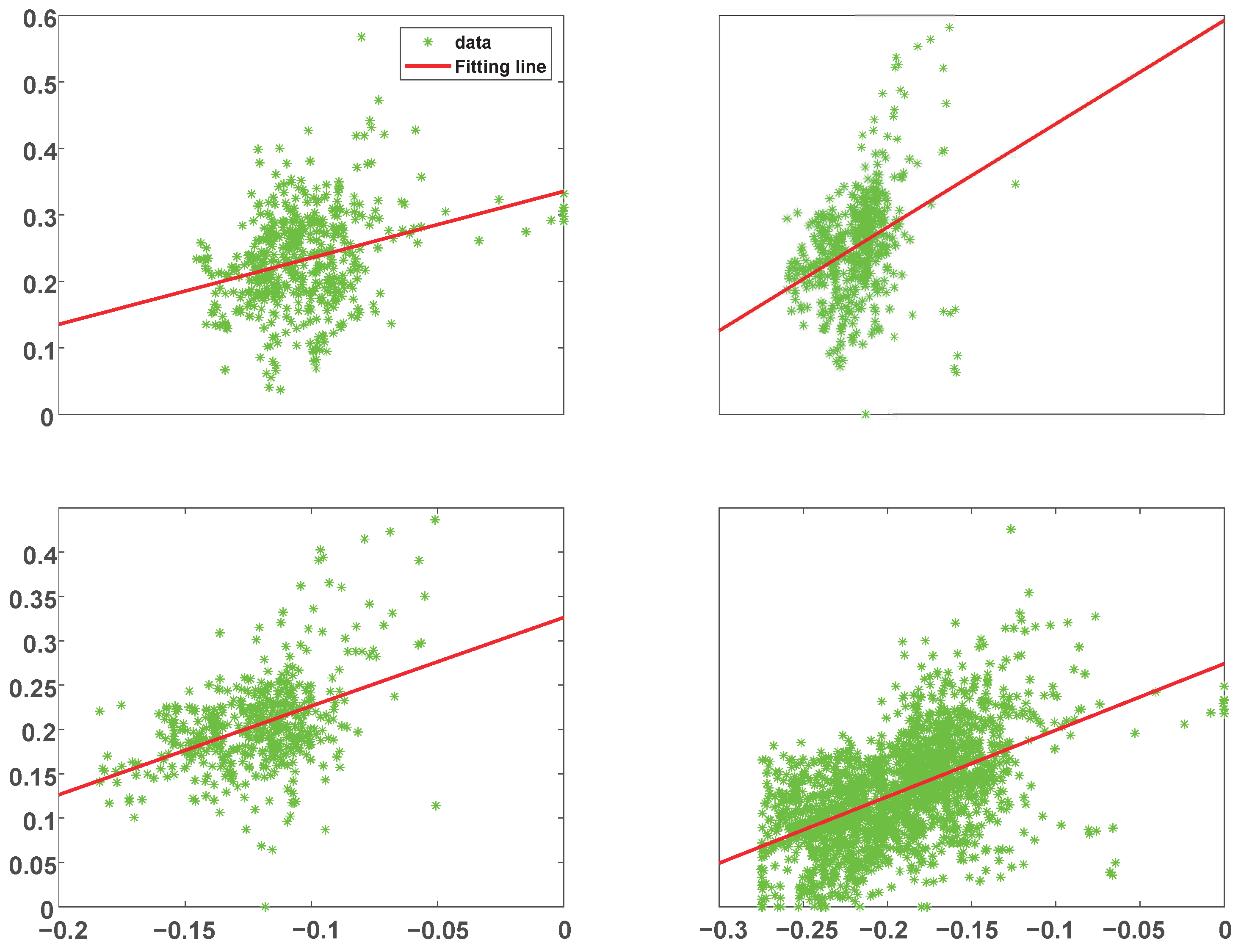
sample 4	−0.274	−0.037	0.36558

below. The sample fitting of the combined variables of noise, vehicle speed, and heading-angle error is established as shown in Figure 1 below. In Figure 1, the abscissa ($f(dhead,v)$) represents a binary function, which is described as $\alpha \ast v_{od}+\beta \ast {\delta }_r$.

Based on the above fitting results, it is not difficult to find that a large number of data points are distributed near the fitting line. This is because the speed and heading angle changes are artificially controlled, that is, the data have an unexplainable fixed variation, and the sample points cannot show functional changes. By adjusting the adaptive factor, or the uncertainty of prediction, the intercept of the fitting line can be changed to approximately coincide with the sample points, and the fitting error can be greatly reduced. Because the accuracy of the noise prediction value does require a high value, it is not necessary to pay attention to the goodness of fit ($R^2$) (R-Square). The relevant evaluation indicators are shown in

Table 3. Regression model evaluation metrics. Here, Dof represents degree of freedom, corresponding to the number of sample points; MSE represents mean square error; RMSE represents root mean square error; and p represents the residual normality test.

	Dof	MSE	RMSE	p
sample 1	497	0.0048	0.0695	0.3644
sample 2	497	0.0022	0.0468	0.0953
sample 3	497	0.0025	0.0500	0.2334
sample 4	1997	0.0041	0.0644	0.0512

below.

Due to the unbounded nature of the residual sum of squares, it is impossible to find an accurate definition to measure its size. Therefore, the mean square error and the root mean square error are used to measure the difference between the predicted value and the true value [20]. The definition is expressed by Equations (14) and (15).

$$MSE={\displaystyle \frac{1}{m}}\underset{i=1}{\sum ^m}{(y_i-f\left(x_i\right))}^2$$

(14)

$$RMSE={\displaystyle \frac{1}{n}}\sqrt{\underset{i=1}{\sum ^n}{(y_i-f\left(x_i\right))}^2}$$

(15)

The MSE of the four groups of samples in the above table is less than 0.01, and the RMSE is less than 0.1, indicating that the sample regression fitting effect is good and the the difference between the predicted value and the true value is small, which can be completely compensated for by the error adaptive factor. The residual normality test is conducted to verify the applicability of the binary regression model. It is generally believed that when the test probability is p > 0.05, it conforms to the normal distribution at the 95% significance level [21]. Therefore, the four sample residuals are normal, and the binary linear regression model is applicable. The residual normal fitting based on the four sample residuals is shown in Figure 2.

To further validate the applicability of the model, it is also necessary to determine whether the residuals of the regression model are independent of each other. Residual independence is an important assumption of linear regression models, and the residuals not being independent may affect the validity of the model and its prediction accuracy [22]. In this paper, we use the Durbin–Watson test to test whether the residuals of the regression model have first-order autocorrelation. This statistic is determined by the following equation:

$$DW={\displaystyle \frac{{\sum }_{t=2}^n{(e_t-e_{t-1})}^2}{{\sum }_{t=1}^n{e}_t^2}}$$

(16)

where $e_t$ is the residual of the tth observation and n is the sample size.

The residuals were obtained by fitting the experiment to four sets of samples; then, the Durbin–Watson statistic was calculated, as summarized in

Table 4. Durbin–Watson volume statistics.

	Sample 1	Sample 2	Sample 3	Sample 4
DW	1.896	1.922	2.112	1.995

.

The Durbin–Watson statistic takes values between 0 and 4, and its value is related to the autocorrelation of the residuals as follows:

➀ When $DW\approx 2$, there is no first-order autocorrelation of the residuals, that is, the residuals are independent of each other, and there is no obvious dependence between the residuals.

➁ When $DW\approx 0$, there is a positive autocorrelation of the residuals. This means that two neighboring residuals are correlated in the same direction, indicating that the sample residuals are not independent of each other.

➂ When $DW\approx 4$, there is a negative autocorrelation of the residuals. This indicates that there is an inverse correlation between two neighboring residuals: one positive and one negative. In the table of sample residual statistics, it can be seen that the DW of all four groups of samples is close to 2, which indicates that the sample residuals are independent of each other, that the samples are well-fit, and that this regression model is applicable.

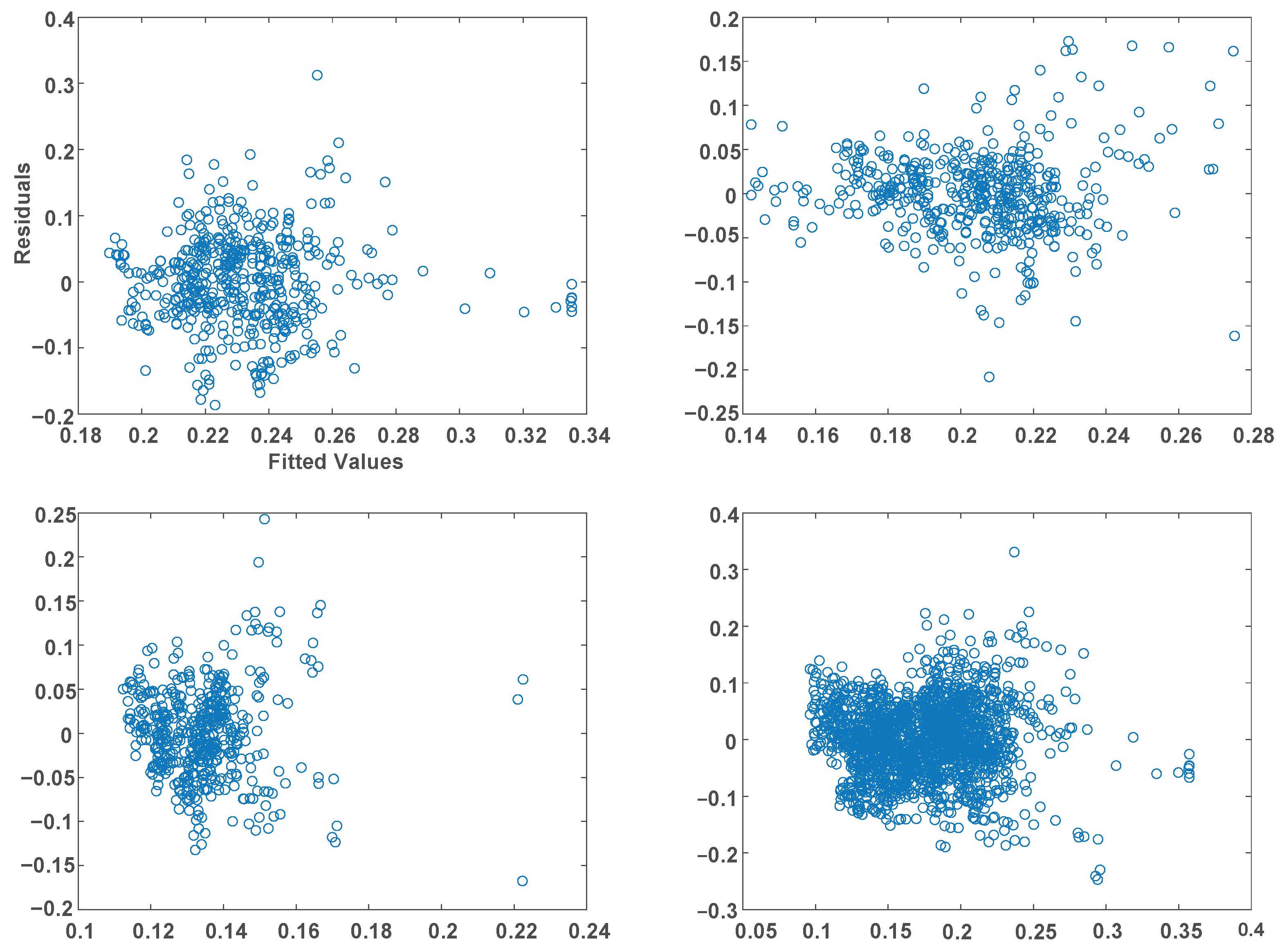
The applicability of the model needs to be further judged in terms of chi-square variance. Chi-square variance indicates that the error term has the same variance at different levels of the independent variable. In this paper, we determine this property using the residual-fitted value plot method. The sample residuals and fitted values are obtained by sample fitting as shown in Figure 3, which shows that the residuals are uniformly distributed around the zero value and have no obvious relationship with the fitted values, which indicates that the variables are variance-aligned.

Finally, based on the above results, we verified the applicability of the model in terms of sample residual normality, residual independence, and variable chi-square variance. The error between the predicted value and the real value is shown in Figure 4. It is easy to determine that the dynamic range of the error is (−0.3, 0.2). The error adaptive factor only needs to be adjusted within this range to compensate for the error of the established binary linear regression model, and the NHC lateral velocity noise can be accurately set. Subsequent experiments show that the error adaptive factor is adjusted within the range, especially at the turning moment, which reduces the positioning error to a certain extent. The model can achieve adaptive NHC noise adjustment, but there are some limitations. Firstly, the model is more sensitive to extreme values, and the extreme values of the data may have a greater impact on the fitting results of the model, making it necessary to preprocess the data in advance. Secondly, the multiple linear regression model is more demanding on the data, and it is necessary to go through the validation of multiple properties before determining its applicability.

In summary, the binary linear regression model is suitable for the adaptive adjustment of NHC lateral velocity noise. This model not only establishes the equivalent relationship between noise, vehicle speed, and heading-angle error but also more accurately determines the setting method of NHC lateral velocity noise and determines the adjustment range of the error adaptive factor.

4. Adaptive Filtering Algorithm Based on Gaussian–Student’s T Mixed Distribution NHC Noise Model

4.1. NHC Lateral Velocity Noise Modeling

The length of the experimental data used in this part is 2000 s. The experimental equipment and experimental scene are shown in the fourth section of the experimental analysis. During this period, the vehicle passes through five large-scale turning sections before and after 193 s, 415 s, 533 s, 790 s, and 996 s. Among them, the 533 s section is a continuous turn. It also passes through some road potholes. The NHC lateral noise model can be analyzed from the following two perspectives:

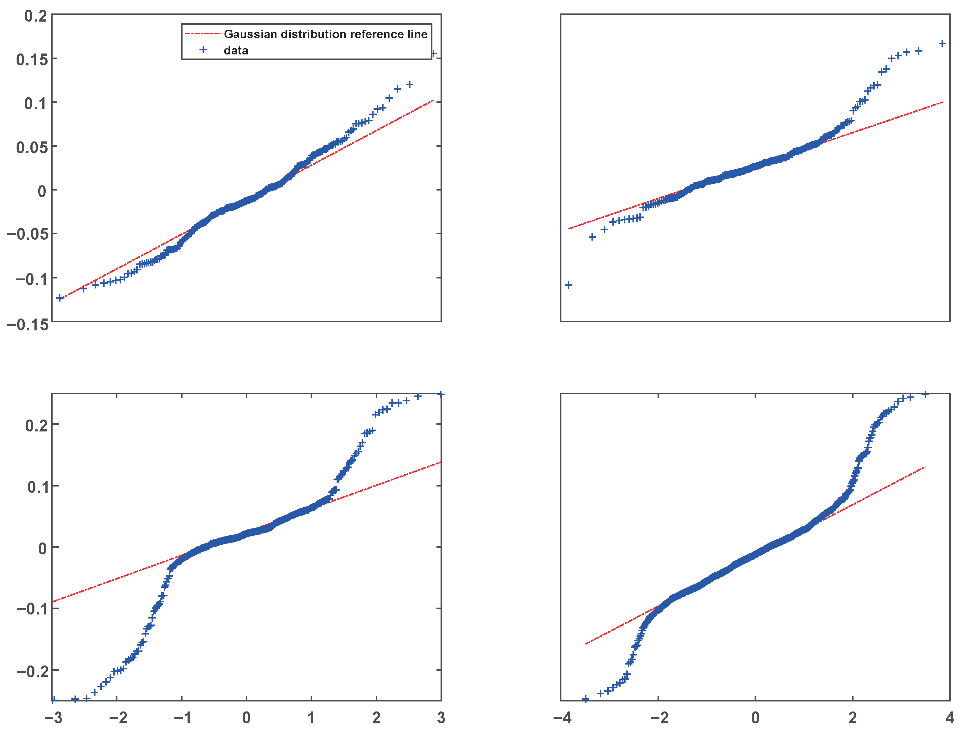
➀ A Quantile–Quantile Plot (Q-Q plot) can directly reflect the degree of agreement between random sequences and the Gaussian distribution [23,24]. The closer the sample curve is to the Gaussian distribution reference line, the closer the sample sequence is to the Gaussian distribution. After obtaining the NHC lateral velocity noise, the Q-Q diagrams for 100–250 s, 350–600 s, and 750–1000 s and the overall experimental data are drawn as shown in Figure 5. The first three time periods contain five turning sections each. It can be seen that in most periods, the NHC lateral velocity noise can be modeled by a Gaussian distribution during the smooth driving of the vehicle. However, once the vehicle turns or slides, the Q-Q diagram shows that it is unreasonable to use the Gaussian model.

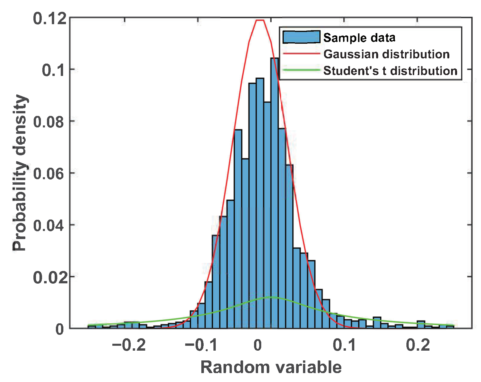
➁ The probability density of NHC lateral velocity noise is shown in Figure 6, and the Gaussian distribution and Student’s T distribution are used for fitting. It can be seen from the figure that the noise has obvious thick-tail characteristics, and the Gaussian distribution curve cannot correctly fit the abnormal noise, so it is unreasonable to only use the Gaussian distribution. Although the T-distribution curve takes into account the tail noise, when the vehicle is running smoothly, the noise is close to the Gaussian distribution. At this time, the velocity noise matrix error is too large to make full use of the NHC observation information, which leads to the loss of accuracy. Based on the above considerations, combined with Figure 4, it can be concluded that modeling the NHC lateral velocity noise as a Gaussian–Student’s T mixed distribution can better reflect the actual noise distribution characteristics and provide more accurate prior information.

Refs. [25,26] proposed a Gaussian–Student’s T mixed noise model. These references considered the conjugate prior of the Bernoulli distribution is as a Beta distribution. In order to facilitate the representation of the mixed probability model as a hierarchical Gaussian form, the mixed probability (${\tau }_k$) is approximated as a Beta distribution in this paper. In fact, the Gaussian–Student’s T mixed probability is approximated as a Beta distribution. On this basis, considering that the NHC is well observed and the NHC is not established, the NHC lateral velocity noise is modeled as a Gaussian–Student’s T mixture model with mixing probability, and the mixing probability is adaptively adjusted according to the vehicle turning and singular velocity detection results. The distribution characteristics are described in Equation (17):

$$p\left(v_k\right)={\tau }_{k}N(v_k;0,R_k)+(1-{\tau }_k)St(v_k;0,R_k,\zeta )$$

(17)

Here, $N(v_{k;}0,R_k)$ represents the zero mean; the variance is the Gaussian distribution of $R_k$; $St(v_k;0,R_k,\varsigma )$ represents the zero-mean Student’s T distribution; $R_k$ is the scale matrix; and $\varsigma$ is the degree of freedom, which is used to describe the fat-tailed degree of noise.

4.2. Mixed State Space Model with Time-Varying and Heavy-Tailed Measurement Noise

The linear discrete state space model can be described as (18) and (19):

$$x_k={\varphi }_{k|k-1}{x}_{k-1}+{\mathrm{\Gamma }}_{k-1}{\omega }_{k-1}$$

(18)

$$z_k=H_k{x}_k+v_k$$

(19)

In the formula, subscripts $k-1$ and k denote times $t_{k-1}$ and $t_k$, respectively, and $x_k$ denotes the state vector (n × 1) at time $t_k$. ${\varphi }_{k|k-1}$ is the one-step state transition matrix (n × n) from $t_{k-1}$ to $t_k$. ${\mathrm{\Gamma }}_{k-1}$ is the system noise driving matrix (n × s), $z_k$ is the observation vector at time $t_k$ (m × 1), $H_k$ is the observation matrix (m × n), ${\omega }_{k-1}$ is the system excitation noise (s × 1), and $v_k$ is the measurement noise (m × 1).

According to Equation (16), the measurement noise and one-step prediction error are modeled as a Gaussian–Student’s T mixed distribution. Since the Student’s T distribution can be regarded as an infinite superposition of the Gaussian distribution, the state space model’s likelihood PDFand one-step prediction PDF are expressed by (20) and (21), respectively:

$$\begin{array}{cc}\hfill & p\left(z_k\right|x_k,{\tau }_k,{\mu }_k)={\tau }_{k}N(z_k;H_k,R_k)\hfill \\ \hfill & +(1-{\tau }_k)N(z_k;H_k{x}_k,R_k,{\displaystyle \frac{\zeta }{{\mu }_k}})\hfill \end{array}$$

(20)

$$\begin{array}{cc}\hfill & p\left(x_k\right|z_{1:k-1},{\gamma }_k,{\psi }_k)={\gamma }_{k}N(x_k;{\varphi }_{k|k-1}{z}_{1:k-1},{\mathrm{\Gamma }}_{k-1}{\omega }_{k-1})+\hfill \\ \hfill & (1-{\gamma }_k)N(x_k;{\varphi }_{k|k-1}{z}_{1:k-1},{\mathrm{\Gamma }}_{k-1}{\omega }_{k-1},{\displaystyle \frac{\sigma }{{\psi }_k}})\hfill \end{array}$$

(21)

where ${\mu }_k$ and ${\psi }_k$ are auxiliary random variables that obey the Gamma distribution ($G(•)$) in the conjugate exponential distribution family. The Gamma distribution is also selected as the prior distribution of $\zeta$ and $\sigma$, expressed as (22)–(25), respectively:

$$p\left({\mu }_k\right)=G({\mu }_k;{\displaystyle \frac{\zeta }{2}};{\displaystyle \frac{\zeta }{2}})$$

(22)

$$p\left({\psi }_k\right)=G({\psi }_k;{\displaystyle \frac{\sigma }{2}};{\displaystyle \frac{\sigma }{2}})$$

(23)

$$p\left(\zeta \right)=G(\zeta ;{\alpha }_1;{\beta }_1)$$

(24)

$$p\left(\sigma \right)=G(\sigma ;{\alpha }_2;{\beta }_2)$$

(25)

In Equation (16), the Gaussian–Student’s T mixed distribution is expressed as a hierarchical Gaussian form. In order to further quantitatively distinguish between a good NHC observation and NHC failure, the Bernoulli random variable ($\eta$) is introduced to represent these two cases, and the Bernoulli probability mass function is used to skillfully fuse the two-layer Gaussian expression of Equation (16). Therefore, the likelihood PDF of Equation (19) and the one-step prediction error PDF of Equation (20) are rewritten as Equations (26) and (27), respectively:

$$\begin{array}{cc}\hfill & p\left(z_k\right|x_k)=\int \int p\left({\tau }_k\right)p\left(\eta \right|{\tau }_k)\hfill \\ \hfill & {\displaystyle \frac{{\left[N(z_k;H_k{x}_k,R_k)\right]}^{\eta }}{{\left[N\left(z_k;H_k{x}_k,R_k,\frac{\zeta }{{\mu }_k}\right)G\left({\mu }_k;\frac{\zeta }{2};\frac{\zeta }{2}\right)\right]}^{\eta -1}}}d{\tau }_{k}d{\mu }_k\hfill \end{array}$$

(26)

$$\begin{array}{cc}\hfill & p\left(x_k\right|z_{1:k-1})=\int \int p\left({\gamma }_k\right)p\left(\rho \right|{\gamma }_k)\hfill \\ \hfill & {\displaystyle \frac{{\left[N(x_k;{\varphi }_{k|k-1}{z}_{1:k-1},{\mathrm{\Gamma }}_{k-1}{\omega }_{k-1})\right]}^{\rho }}{{\left[N\left(x_k;{\varphi }_{k|k-1}{z}_{1:k-1},{\mathrm{\Gamma }}_{k-1}{\omega }_{k-1},\frac{\sigma }{{\psi }_k}\right)G\left({\psi }_k;\frac{\sigma }{2};\frac{\sigma }{2}\right)\right]}^{\rho -1}}}\hfill \\ \hfill & d{\psi }_{k}d{\gamma }_k\hfill \end{array}$$

(27)

where $\eta \in \{1,0\},\rho \in \{1,0\}$ and the corresponding probability mass functions are expressed as (28) and (29):

$$p\left(\eta \right|{\tau }_k)={\displaystyle \frac{{\tau }_k^{\eta }}{{(1-{\tau }_k)}^{\eta -1}}}$$

(28)

$$p\left(\rho \right|{\gamma }_k)={\displaystyle \frac{{{\gamma }_k}^{\rho }}{{(1-{\gamma }_k)}^{\rho -1}}}$$

(29)

The mixing probabilities (${\tau }_k$) are updated at each iteration based on the variational lower-bound maximization principle. The update formula is expressed as Equation (30):

$${\tau }_k={\displaystyle \frac{1}{N}}\sum _{n=1}^N{\mathbb{E}}_{q\left(z_n\right)}\left[z_{nk}\right]$$

(30)

where $z_n$ is an indicator variable, i.e., it indicates which distribution the current data belong to, and ${\mathbb{E}}_{q\left(z_n\right)}\left[z_{nk}\right]$ is the expectation of the data ($q\left(z_n\right)$) under the variational distribution. The equation can be decomposed into two parts. The first part involves calculating the a posteriori probability of the kth ephemeral datum in each sliding window, then updating the hybrid probability based on the principle of maximizing the lower bound of the variational division; then with the iteration, the hybrid probability eventually converges to a stable value that is most consistent with the actual state of the vehicle’s movement so as to achieve an accurate fit to the distribution of the data. Sometimes, in order to prevent overfitting, we generally introduce a priori distributions, such as the Dirichlet distribution, to the mixed probability. Finally, the mixing probability is normalized based on the maximum value, enabling adaptive adjustment of the mixing probability.

Based on the above theory, the mixed-state hierarchical Gaussian model can be described as follows: The NHC side-vector measurement noise and one-step prediction error are modeled as a Gaussian–Student’s T mixed distribution. The Student’s T distribution is approximated as a hierarchical Gaussian distribution with an adjustable scale matrix. The modeling of NHC side-vector measurement noise and one-step prediction error is adjusted by mixing probability. When the NHC is well observed, that is, the vehicle is driving smoothly, it is modeled as a Gaussian distribution, that is, ${\tau }_k,{\gamma }_k=1$; when the NHC fails to a certain extent, that is, the vehicle has a singular speed, especially at the turning moment, it is modeled as the Student’s T distribution, that is, ${\tau }_k,{\gamma }_k=0$.

4.3. Parameter Update and Posterior Approximation Based on Variational Bayesian (VB)

VB method is an approximate method for obtaining the approximate solution of the joint posterior probability density of a state vector and unknown parameters [27]. Based on the establishment of the state space model, the VB method makes full use of the observation information and prior information to find the approximate solution ($q(X,\theta )$) of the joint posterior probability density of the state vector to be estimated and the unknown parameter. In this way, it can approximate the exact solution of the joint posterior probability density ($p(X,\theta |Z)$ where X represents the state vector to be estimated, $\theta$ represents the unknown parameter, and Z represents the known observation vector) [28].

The VB method needs to model the approximate solution ($q(X,\theta )$) as the conjugate distribution form of the likelihood function. Using the conjugate distribution characteristics, the calculation can be simplified to obtain the analytical solution of the posterior distribution. Secondly, the VB method makes a one-step approximation of the coupling relationship between variables, which can be expressed as shown in Equation (31).

$$q(X,\theta )=q\left(X\right)\underset{i=1}{\prod ^n}q\left({\theta }_i\right)$$

(31)

KL divergence is an evaluation method for the difference between probability distributions. The VB method uses the Kullback–Leibler Divergence (KLD) method to minimize the KL divergence between the two distributions so that $q(X,\theta )$ approaches $p(X,\theta |Z)$ to the maximum extent:

$$q^{\ast }\left(\varphi \right)=argminKLD(q\left(X\right)\underset{i=1}{\prod ^n}q\left({\theta }_i\right)\left|\right|p(X,{\theta }_i|z_{1:k}))$$

(32)

Here, $q^{\ast }\left(\varphi \right)$ is the approximate posterior probability density, and $z_{1:k}$ is the observation information at 1:ktime. In Ref. [29], Equation (17) was deduced and calculated in detail by using the VB method. It was concluded that any posterior probability density of the state vector to be estimated and the unknown parameters can be expressed by Equation (33):

$$lnq\left(\epsilon \right)=E_{{\mathrm{\Theta }}^{-\epsilon }}[lnp(\mathrm{\Theta },z_{1:k})]+const$$

(33)

In the formula, $\mathrm{\Theta }$ is the set of the state vector to be estimated and the unknown parameters, that is, $\mathrm{\Theta }\triangleq \{X,{\theta }_i\}$; $\epsilon$ is any element in the set; and $E_{{\mathrm{\Theta }}^{-\epsilon }}[•]$ represents the expectation of all random variables in the set except $\epsilon$ [30].

The above formula is the core of the VB method. After providing the prior information of the parameters to be estimated, the updated formula of each parameter can be obtained through Formula (31), that is, the current posterior information. The posterior information is used as the filter input for the prior information of the next moment, and the iteration is carried out continuously. Since the above formula cannot obtain the analytical solution, the fixed-point iteration is usually used to solve for the local optimal solution of $q\left(\epsilon \right)$ [30,31,32].

Since the joint posterior probability density function ($p(x_k,{\mu }_k,{\psi }_k|z_{1:k-1})$) usually has difficulty in obtaining a closed analytical solution, based on the idea of the VB method, it is necessary to find the approximation of its free decomposition [33,34], as shown in Equation (34).

$$p(x_k,{\mu }_k,{\psi }_k|z_{1:k-1})\approx q\left(x_k\right)q\left({\mu }_k\right)q\left({\psi }_k\right)$$

(34)

The next goal is to find the optimal solution of Equation (30) using the KLD method, which is expressed as, $\mathrm{\Theta }\triangleq \{x_k,{\mu }_k,{\psi }_k\}$, while the joint PDF can be written as Equations (35)–(38).

$$p(\mathrm{\Theta },z_{1:k})=p\left(z_{1:k-1}\right)p\left(z_k\right|x_k)p\left(x_k\right|z_{1:k})$$

(35)

$$p\left(z_{1:k-1}\right)=N(z_{1:k-1};H_k{x}_{1:k-1},R_k)$$

(36)

$$\begin{array}{cc}\hfill & p\left(z_k\right|x_k)={\displaystyle \frac{{\left[N(z_k;H_k{x}_k,R_k)\right]}^{\eta }}{{\left[N\left(z_k;H_k{x}_k,R_k,\frac{\zeta }{{\mu }_k}\right)G\left({\mu }_k;\frac{\zeta }{2};\frac{\zeta }{2}\right)\right]}^{\eta -1}}}\hfill \\ \hfill & \ast {\displaystyle \frac{{\tau }_k^{\eta }}{{(1-{\tau }_k)}^{\eta -1}}}\hfill \end{array}$$

(37)

$$\begin{array}{cc}\hfill & p\left(x_k\right|z_{1·k})={\displaystyle \frac{{\left[N(x_k;{\widehat{x}}_{k|k-1},{\widehat{P}}_{k|k-1})\right]}^{\rho }}{{\left[N\left(x_k;{\widehat{x}}_{k|k-1},\frac{{\widehat{P}}_{k|k-1}}{{\psi }_k}\right)G\left({\psi }_k;\frac{\sigma }{2};\frac{\sigma }{2}\right)\right]}^{\rho -1}}}\hfill \\ \hfill & \ast {\displaystyle \frac{{{\gamma }_k}^{\rho }}{{(1-{\gamma }_k)}^{\rho -1}}}\hfill \end{array}$$

(38)

By substituting Formula (35) into Formula (33), the state vector update Formula (39) can be obtained as

$$q^{(i+1)}\left(x_k\right)=N\left(x_k;{\widehat{x}}_{k|k}^{(i+1)},{\widehat{P}}_{k|k}^{(i+1)}\right)$$

(39)

where $q^{i+1}(·)$ represents the approximate value of the ($i+1$)th iteration. The mean value of the state vector iteration (${\widehat{x}}_{k|k}^{(i+1)}$) and the covariance matrix (${\widehat{P}}_{k|k}^{(i+1)}$) can be determined by Equations (40)–(42).

$$K_k^{(i+1)}={\widehat{P}}_{k|k-1}^{(i+1)}{H}_k^T{\left(H_k{\widehat{P}}_{k|k-1}^{(i+1)}{H}_k^T+{\widehat{R}}_k^{(i+1)}\right)}^{-1}$$

(40)

$${\widehat{x}}_{k|k}^{(i+1)}={\widehat{x}}_{k|k-1}+K_k^{(i+1)}(z_k-H_k{\widehat{x}}_{k|k-1})$$

(41)

$${\widehat{P}}_{k|k}^{(i+1)}={\widehat{P}}_{k|k-1}^{(i+1)}-K_k^{(i+1)}{H}_k{\widehat{P}}_{k|k-1}^{(i+1)}$$

(42)

According to the definition of a Bernoulli distribution, the expectation of a Bernoulli random variable ($\eta ,\rho$) is expressed as (43) and (44):

$$E\left(\eta \right)=\sum _{x\in Val\left(\eta \right)}xp\left(x\right)={\tau }_k$$

(43)

$$E\left(\rho \right)=\sum _{x\in Val\left(\rho \right)}xp\left(x\right)={\gamma }_k$$

(44)

The mixing probability (${\tau }_k,{\gamma }_k$) is set according to whether the NHC has a certain degree of failure. When the vehicle is running smoothly and there is no singular speed in the lateral or celestial direction, ${\tau }_k={\gamma }_k=1$ and 0 otherwise.

In (38) and (40), the one-step prediction covariance matrix (${\widehat{P}}_{k|k-1}^{(i+1)}$) and the measurement noise matrix (${\widehat{R}}_k^{(i+1)}$) can be determined by (45) and (46) [35,36].

$${\widehat{P}}_{k|k-1}^{(i+1)}={\displaystyle \frac{{\widehat{P}}_{k|k-1}^{\left(i\right)}}{\frac{cons{t}^{E\left(\eta \right)}}{E^{\left(i\right)}{\left[{\mu }_k\right]}^{\left(E\right(\eta )-1)}}}}$$

(45)

$${\widehat{R}}_k^{(i+1)}={\displaystyle \frac{{\widehat{R}}_k^{\left(i\right)}}{\frac{cons{t}^{E\left(\rho \right)}}{E^{\left(i\right)}{\left[{\psi }_k\right]}^{\left(E\right(\rho )-1)}}}}$$

(46)

According to Equation (35), $q^{(i+1)}\left({\mu }_k\right)$ is updated by the Gamma distribution, and Equations (47)–(50) can be obtained as follows:

$$q^{(i+1)}\left({\mu }_k\right)=G\left({\mu }_k;{\xi }_k^{(i+1)},{\sigma }_k^{(i+1)}\right)$$

(47)

$${\xi }_k^{(i+1)}={\displaystyle \frac{\zeta }{2}}+{\displaystyle \frac{cons{t}^{E\left(\eta \right)}}{0.5n^{\left(E\right(\eta )-1)}}}$$

(48)

$${\sigma }_k^{(i+1)}={\displaystyle \frac{\zeta }{2}}+{\displaystyle \frac{cons{t}^{E\left(\eta \right)}}{0.5tr{\left(A_k^{(i+1)}{\widehat{P}}_{k|k-1}^{(-1)}\right)}^{\left(E\right(\eta )-1)}}}$$

(49)

$$A_k^{(i+1)}={\widehat{P}}_{k|k}^{(i+1)}+\left({\widehat{x}}_{k|k}^{(i+1)}-{\widehat{x}}_{k|k-1}\right){\left({\widehat{x}}_{k|k}^{(i+1)}-{\widehat{x}}_{k|k-1}\right)}^T$$

(50)

where $tr(·)$ denotes the trace of the matrix and $E^{(i+1)}\left[{\mu }_k\right]$ is updated by Equation (51).

$$E^{(i+1)}\left[{\mu }_k\right]={\xi }_k^{(i+1)}{\sigma }_k^{{(i+1)}^{-1}}$$

(51)

Similarly, $q^{(i+1)}\left({\psi }_k\right)$ is also updated by the Gamma distribution, and $E^{(i+1)}\left[{\psi }_k\right]$ is updated as follows ((52)–(56)):,

$$q^{(i+1)}\left({\psi }_k\right)=G\left({\psi }_k;{\omega }_k^{(i+1)},{\phi }_k^{(i+1)}\right)$$

(52)

$${\omega }_k^{(i+1)}={\displaystyle \frac{\sigma }{2}}+{\displaystyle \frac{cons{t}^{E\left(\rho \right)}}{0.5m^{\left(E\right(\rho )-1)}}}$$

(53)

$${\phi }_k^{(i+1)}={\displaystyle \frac{\sigma }{2}}+{\displaystyle \frac{cons{t}^{E\left(\rho \right)}}{0.5tr{\left(B_k^{(i+1)}{\widehat{R}}_k^{{\left(i\right)}^{-1}}\right)}^{\left(E\right(\rho )-1)}}}$$

(54)

$$B_k^{(i+1)}=H_k{\widehat{P}}_{k|k}^{(i+1)}{H}_k^T+\left(z_k-H_k{\widehat{x}}_{k|k}^{(i+1)}\right){\left(z_k-H_k{\widehat{x}}_{k|k}^{(i+1)}\right)}^T$$

(55)

$$E^{(i+1)}\left[{\psi }_k\right]={\omega }_k^{(i+1)}{\phi }_k^{{(i+1)}^{-1}}$$

(56)

We analyze the computational complexity of the algorithm in terms of the number of model parameters in the initialization phase of the algorithm, the time complexity of calculating the a priori mean, and the noise covariance based on the a priori distribution of the predicted state of the system model, as well as the computational time complexity of the parameter-variational approximation phase and the complexity of the update operation, compared to conventional filtering algorithms, such as Kalman filtering and particle filtering, as summarized in

Table 5. Statistical table of computational complexity. n represents the dimension of the covariance matrix, p is the number of variational parameters, q is the complexity of the update operation, m is the dimension of the observation matrix, T is the number of iterations, and N is the number of particles.

	Ga-St VBAKF	EKF	Particle Filter
Complexity of computation	$O\left(T\left(n^3+nm+pq\right)\right)$	$O\left(T{n}^3\right)$	$O(n+n^2)$

. The computational complexity of the algorithm is higher than that of conventional filtering algorithms, and the cost of high computing power is exchanged for better filtering performance [37].

The computational load of the algorithm can be considered in terms of its demand on memory usage, which consists of the posterior probability matrix used for updating the mixing probabilities within the sliding window. Assuming its size to be M × N and each mixing probability size to be K, as well as the variational parameter, and assuming the covariance matrix to be A × A and the rest of the parameters to be in B dimensions, the algorithm’s demand on memory is $O(M\times N+K\times A^2+K\times B)$. The time complexity of the algorithm is related to the convergence rate (T) of the algorithm, the data size (N), the data dimension (M), and the number of variational parameters (K). The total time complexity is $O(T\times N\times K\times M^2)$. The variational Bayesian filtering algorithm is generally more complex compared to other algorithms. The complexity of the algorithm mainly depends on the matrix operation of the mixed probability update; therefore, in the actual operation of the algorithm, we generally use data dimensionality reduction to reduce the actual complexity or, in the mixed probability update, in the lower bound of the variational change to terminate convergence early.

So far, all parameters of the adaptive filtering algorithm based on the VB method have been updated. The flow chart of the Ga-St VBAKF algorithm proposed in this section is shown in Algorithm 1 [38,39,40].

Algorithm 1: Ga-St VBAKF algorithm procedure

Input: ${\widehat{x}}_{k-1|k-1}$,${\widehat{P}}_{k-1|k-1}$,${\varphi }_{k|k-1}$,$Q_{k-1}$,$R_k$,$z_k$,            $H_k$, n,m, $\sigma$,$\zeta$,${\tau }_k$,${\gamma }_k$,$a\_ite,b\_ite,c\_ite,d\_ite$,N Time Update: Updated according to standard Kalman filter algorithm            ${\widehat{x}}_{k|k-1},{\widehat{P}}_{k|k-1}$ Measurement Update: 1. Initialization $E\left[{\psi }_k\right],E\left[{\mu }_k\right]$,$E\left(\eta \right),E\left(\rho \right)$,$a\_ite,b\_ite,c\_ite,d\_ite$ 2. Iteration for i = 1:N ➀ Measurement Update according to Equations (38)–(40) ➁ $q^{(i+1)}\left({\mu }_k\right),q^{(i+1)}\left({\psi }_k\right)$ are updated according to Gamma distribution. ➂ According to Equations (41) and (42), $E\left(\eta \right)$ is defined as    $Pr\_1(\mathrm{\Gamma }=1)/(Pr\_1(\mathrm{\Gamma }=1)+Pr\_1(\mathrm{\Gamma }=0\left)\right)$, $E\left(\eta \right)\mathrm{and}E\left(\rho \right)$ are updated.      Here, $Pr\_1(\mathrm{\Gamma }=1,0)$ is updated by Gamma distribution with      $a\_ite,b\_ite,c\_ite,d\_ite$, and then update $a\_ite,b\_ite,c\_ite,d\_ite$.      $A_k^{(i+1)},B_k^{(i+1)}$ are updated according to Equations (48)–(53).      ${\xi }_k^{(i+1)},{\sigma }_k^{(i+1)},{\omega }_k^{(i+1)},{\phi }_k^{(i+1)}$ are updated according to Equations (46) and (47),     (51) and (52).      $E^{(i+1)}\left[{\mu }_k\right],E^{(i+1)}\left[{\psi }_k\right]$ are updated according to Equations (49) and (54). ➃ Updated values will be used in the next iteration. 3. End of loop: ${\widehat{x}}_{k\mid k}={\widehat{x}}_{k\mid k}^N,{\widehat{P}}_{k\mid k}={\widehat{P}}_{k\mid k}^N$.

5. Algorithm Verification

The experiments reported in this paper are vehicle-mounted GNSS/INS combined navigation and positioning experiments, and the test data were collected by a self-developed low-cost combined GNSS/INS navigation module. The MEMS-level IMU chip, the GNSS chip, the microsensor chip, and the microprocessor are integrated into the chip. Some parameters of the IMU chip are shown in

Table 6. Performance parameters of IMU chip on GNSS/INS module.

IMU Chip Index	Parameter
Gyro bias stability	10°/h
Gyroscope angle random walk	0.27°/sqrt(h)
Accelerometer bias stability	1800 mGal
Accelerometer speed random walk	0.042 m/s/sqrt(h)

. To verify the performance of the proposed algorithm, this paper uses the positioning results of a high-precision Novatel SPAN-CPT navigation and positioning instrument as a reference benchmark. This is a combined INS/GNSS navigation and positioning system that houses NovAtel’s high-end GNSS board and an IMU component consisting of a fiber-optic gyro and a MEMS accelerometer, and its performance parameters are shown in

Table 7. Positioning accuracy of SPAN-CPT.

Index of Precision	Parameter
Dual-frequency RTK	1 cm + 1 ppm
Heading-angle RMS	0.06°
Pitch RMS and roll RMS	0.02°
X, Y, and Z speed accuracy	0.03 m/s

,

Table 8. Performance index of SPAN-CPT gyroscope.

Performance Index	Parameter
Measuring range	±375°/s
Deviation	±20°/h
Deviation stability	±1°/h
Precision of scale factor	1500 ppm
Random walk	0.0667°/sqrt(h)

and

Table 9. Performance index of SPAN-CPT gyroscope.

Performance Index	Parameter
Measuring range	±10 g
Deviation	50 mg
Deviation stability	±0.75 mg
Precision of scale factor	4000 ppm

. Before verifying the performance of the algorithm, we first performed a series of preprocessing steps on the data. Firstly, the vehicle speed and heading angle in the data collected by the GNSS/INS module were used to obtain the value of the heading-angle change and vehicle speed in the carrier coordinate system for fitting experiments, and the fitting noise was used as the initial value of noise for adaptive adjustment in the positioning experiments. Secondly, the turning moments of the vehicle were obtained by the turn detection algorithm, and the experiments were focused on the change of the vehicle positioning accuracy at these moments. With this positioning experiment, we need to verify that the algorithm maximizes the performance of the NHC in turning sections and improves the GNSS/INS positioning results in complex scenes.

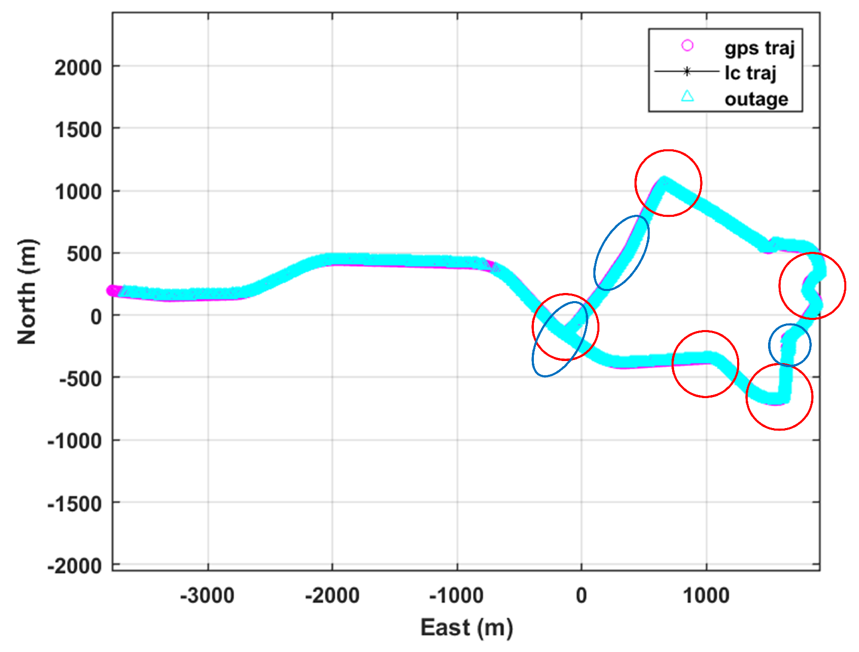
The data used in this paper were collected by vehicle-mounted INS/GNSS integrated navigation equipment in a complex urban environment. The total duration is 2000 s. The driving path is shown in Figure 7. The driving path includes five sections of turning sections, including a section of continuous turning sections (indicated by red marks); three sections of pavement potholes (blue marks); and eight weak-signal scenarios such as boulevards, tunnels, and mountainside. The driving environment is complex, and the collected data can give full play to the adaptive adjustment method of NHC lateral noise and the Ga-St VBAKF algorithm.

5.1. Experimental Design

In order to verify the effectiveness of the proposed algorithm, this paper sets up two experimental groups and five control groups, as shown in

Table 10. The table represents the complete experimental design. It should be noted that in the following text, these groups are defined as ➀➁➂➃➄➅➆.

	GNSS	${\mathit{\sigma }}_{\mathit{x}}$	Gaussian Distribution	Mixed Distribution
Experimental group 1	✓	self-adaptation		✓
Control group 1	✓	fixation		✓
Control group 2	✓	self-adaptation	✓
Control group 3	✓	fixation	✓
Experimental group 2	×	self-adaptation		✓
Control group 4	×	fixation		✓
Control group 5	×	self-adaptation	✓

.

In the experiment in which the GNSS signal is effective, experimental group 1 and control group 1 are used to illustrate the effectiveness of the adaptive adjustment method of NHC lateral velocity noise. Experimental group 1 and control group 2 are used to illustrate the superiority of the Ga-St VBAKF algorithm. Control group 3 can be used as the reference of experimental group 1 and control groups 1 and 2 to illustrate the effectiveness of the NHC lateral velocity noise adaptive adjustment method and the Ga-St VBAKF algorithm. According to the vehicle turning judgment algorithm and speed detection method presented in the second section, in this section of 2000 s of data, the vehicle turns at 193 s, 415 s, 533 s, 790 s, and 996 s, and there are 22 vehicles with lateral singular speed and 28 with vertical singular speed. The turning time of the vehicle is delayed by 15 s before and after the time point when the heading-angle change value and the vehicle speed reach the threshold. In order to verify the applicability of the algorithm when the vehicle is driving in a complex scene, especially in a turning state or with a singular speed, we designed experimental group 2. In experimental group 2, through artificial simulation, the 30 s GNSS signal interruption is implemented before and after the five-section turning of the vehicle, which indicates the auxiliary ability of the NHC with respect to pure INS/OD navigation. During the GNSS outage, experimental group 2, control group 4, and control group 5 are used to illustrate the applicability and effectiveness of the adaptive combined filtering algorithm in complex environments. Experimental group 1 and experimental group 2 are also compared to illustrate the influence of the GNSS signal on the combined filtering algorithm. In this paper, the maximum value of the absolute value of the estimation error and the root mean square of the estimation error are used to quantitatively discuss the estimation accuracy of each group. The definition is shown in Equation (15).

It should be noted that in addition to the difference in the NHC pseudo-measurement noise covariance matrix, the remaining parameters that affect the accuracy (such as the system noise covariance matrix, GNSS position observations, odometer observations, transfer matrix, etc.) are consistent. In addition, in the experiment investigating the effectiveness of the GNSS signal, the filtering algorithm combined with GNSS observations has a certain anti-noise function, but the focus of this article is not here, so it only needs to be consistent but not discussed.

5.2. Experimental Results and Analysis

The north position estimation error of the whole test is shown in Figure 8. The maximum value of the north position estimation error and the root mean square statistics are shown in

Table 11. North position estimation error statistics. The maximum improvement in the table indicates the case when the GNSS signal is present in the former and the case when the GNSS signal is interrupted in the latter.

North Position/m	➀	➁	➂	➃	Maximum Improvement	➄	➅	➆	Maximum Improvement
RMS	0.28	0.32	0.75	0.82	65.9%	0.71	1.23	1.19	42.3%
MAX	1.32	1.53	3.72	2.92	64.5%	4.55	6.44	6.48	29.8%

. According to the comparison shown in the Figure 8, it can be seen that experimental group 1, control group 1, and control group 2 exhibit a certain improvement in the north position estimation accuracy compared with control group 3. In general, the estimation accuracy of experimental group 1 and control group 1 is better than that of the other two groups. Near the above turning time point, it can be seen that there are gross errors of a certain size in each group. At this time, the lateral or vertical pseudo-measurement noise of NHC/OD begins to increase, and the Kalman filter based on the Gaussian distribution is more sensitive to gross measurement errors, resulting in greater errors. The experimental results shown in Figure 7 were obtained by interrupting the GPS signal when the vehicle turned or when the singular speed occurred. It can be seen that the gross error near the turning time point is further increased. It is obvious that the Ga-St VBAKF algorithm is still superior to other groups in terms of error divergence and divergence speed in the case of GNSS signal interruption.

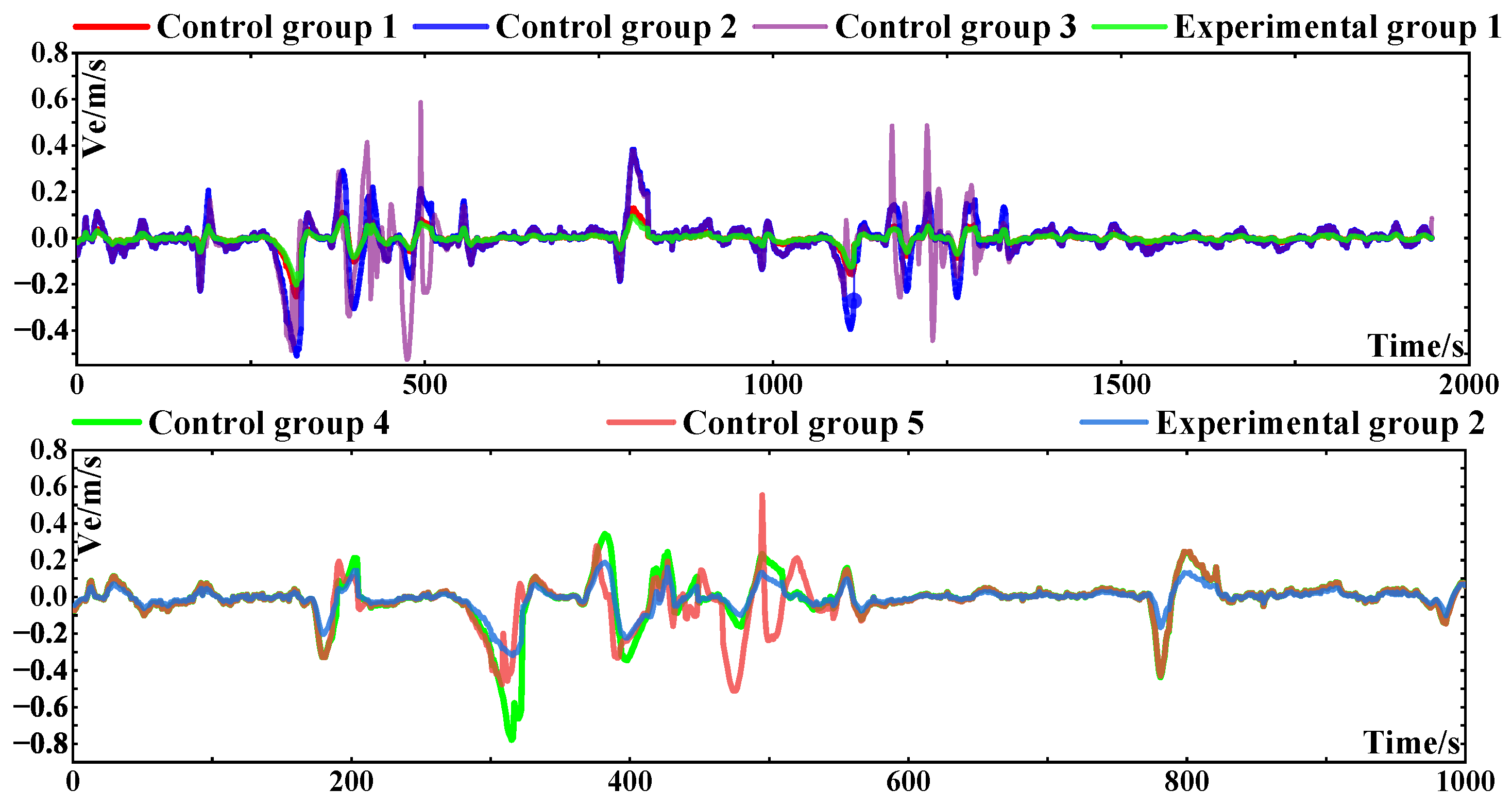
The east position estimation error of the whole test is shown in Figure 9. The maximum value of the position error in the east direction and the root mean square are shown in

Table 12. East position estimation error statistics.

East Position/m	➀	➁	➂	➃	Maximum Improvement	➄	➅	➆	Maximum Improvement
RMS	0.43	0.52	1.15	1.19	63.9%	1.15	1.41	1.63	29.4%
MAX	2.07	2.41	5.59	8.48	75.6%	6.97	7.20	8.00	12.9%

. Based on the upper figure in Figure 8, combined with Table 8, it should be noted that in the vicinity of 500 s, the vehicle continuously passes through complex scenes such as tunnels, mountains, etc., and there are continuous turns, poor road conditions, and large gross errors in GNSS measurement, so the adaptive filter based on the Gaussian distribution for the NHC has little effect on error improvement, which further verifies that the lateral and even vertical pseudo-measurement noise of the NHC under complex road conditions does not simply obey the Gaussian distribution. In the vicinity of the turning time point, it can be seen that the Ga-St VBAKF algorithm with adaptive noise achieves the best performance, while the Ga-St VBAKF algorithm with fixed measurement noise achieves similar performance; however, on the fourth turn, that is, 790 s, it can be clearly seen that the former achieves better performance. As shown in Figure 8, at the second turning point of 415 s, the errors of the three schemes are large because the GNSS signal interruption time is long, which leads to the large error divergence in this section. This is also demonstrated by the north position error in Figure 7. But at the third turning point, it can be clearly seen that when the GNSS signal is interrupted, if the NHC uses the Ga-St VBAKF algorithm with the adaptive noise method to assist the OD/INS integrated navigation, the effect of this method is the largest and the degree of divergence is the smallest.

The ground-position estimation error of the whole test is shown in Figure 10. The maximum value of the ground-position error and the root mean square are shown in

Table 13. Ground-position estimation error statistics.

Ground Position/m	➀	➁	➂	➃	Maximum Improvement	➄	➅	➆	Maximum Improvement
RMS	0.19	0.29	0.28	1.24	84.7%	0.53	0.54	1.34	60.4%
MAX	1.15	1.76	1.75	9.82	88.3%	2.58	2.58	6.71	61.5%

. This part is mainly to verify the effectiveness of the elevation constraint and to verify the effect of the adaptive filter based on the Gaussian–Student’s T mixed distribution in the elevation constraint. At this time, the ground position error is simultaneously affected by the normal velocity correction of the velocity constraint and the sky velocity correction of the elevation constraint. It should be noted that the elevation constraint is not used in control group 3. When the vehicle is bumpy or moving up and down and the road conditions are poor, the vertical velocity of the vehicle is singular. At this time, the fixed vertical velocity noise in the non-integrity constraint is not applicable. In data preprocessing, at 500 s, the vehicle has a singular speed in the vertical direction for many times. During this period (1000–1500 s), the vehicle traveled in pavement-pitted boulevards, underground tunnels, and continuously turning mountain bypasses. It can be seen from the experimental results that the Ga-St VBAKF algorithm used in the elevation constraint achieves better performance than the adaptive filter based on the Gaussian distribution, and the method of adaptively adjusting the vertical velocity noise of the vehicle also has a certain effect. In Figure 9, it is not difficult to determine whether the vertical velocity noise is adaptive and whether the GNSS signal is interrupted; their effects on the ground-position error are not much different. However, when the vehicle has a vertical singular velocity or the GNSS signal is interrupted, the Ga-St VBAKF algorithm, which relies on the elevation constraint condition and the dynamic adjustment of the R matrix, can still minimize the ground-position estimation error.

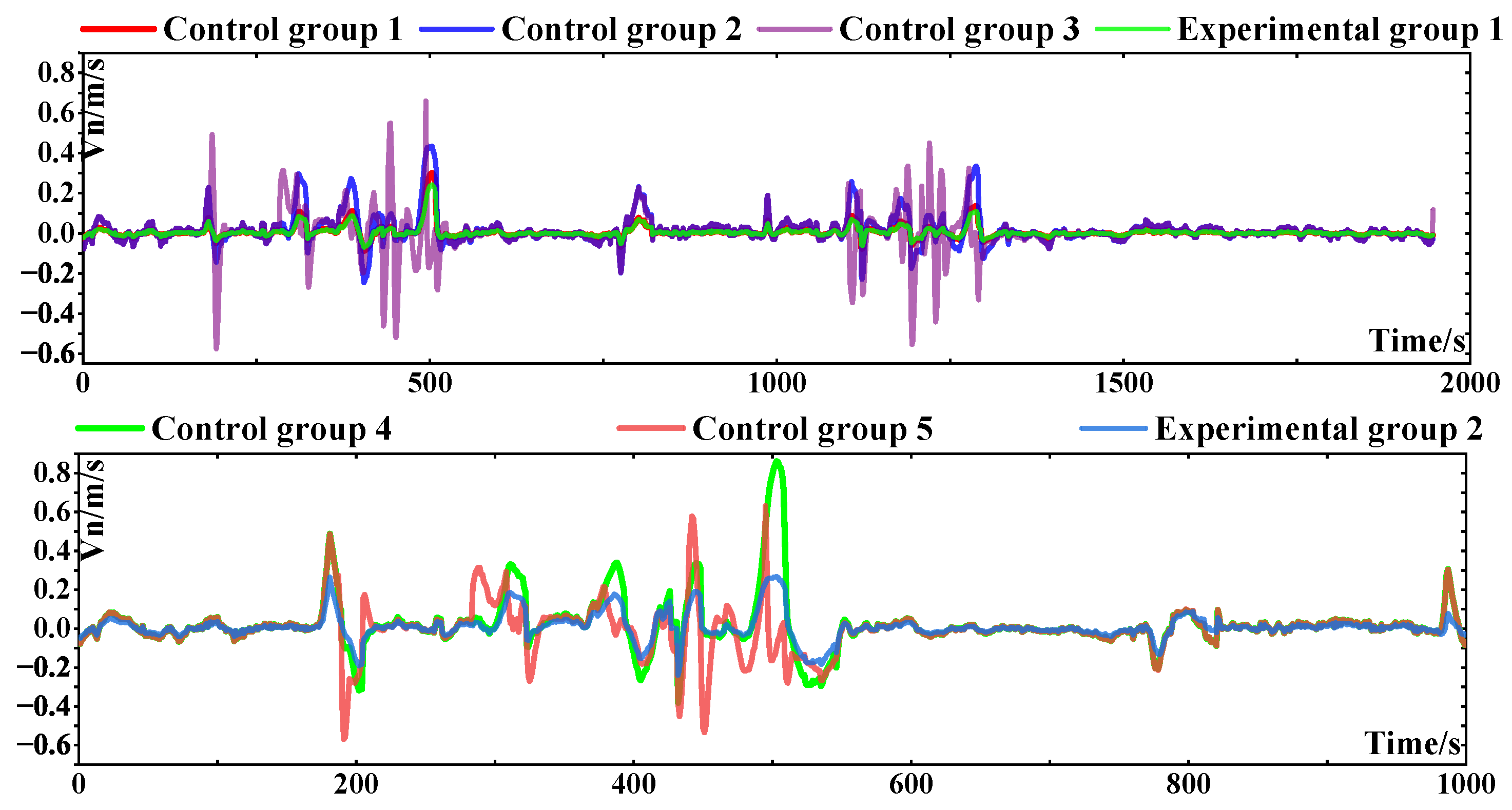
The estimation errors of north velocity and east velocity in the whole test are shown in Figure 11 and Figure 12. The maximum errors of north velocity and east velocity and the root mean square are shown in

Table 14. North velocity estimation error statistics.

North Velocity/m/s	➀	➁	➂	➃	Maximum Improvement	➄	➅	➆	Maximum Improvement
RMS	0.027	0.033	0.077	0.095	71.6%	0.065	0.136	0.027	52.2%
MAX	0.24	0.30	0.43	0.66	63.6%	0.27	0.86	0.63	68.6%

and

Table 15. East velocity estimation error statistics.

East Velocity/m/s	➀	➁	➂	➃	Maximum Improvement	➄	➅	➆	Maximum Improvement
RMS	0.027	0.034	0.090	0.098	72.4%	0.067	0.127	0.115	47.2%
MAX	0.20	0.25	0.51	0.59	66.1%	0.32	0.78	0.55	59%

. In the vicinity of the five turning points described above and during the time period when variable velocity occurs, it can be seen in Figure 11 and Figure 12 that the error dispersion is very fast and reaches about 0.7 m/s in the north direction and 0.6 m/s in the east direction. In the figures in Figure 11 and Figure 12, if the lateral pseudo-measurement noise of the NHC is modeled as a Gaussian–Student’s T mixed distribution and the R matrix is adjusted adaptively in complex sections, the error is greatly reduced. As shown in Figure 11 and Figure 12, the GNSS signal is also interrupted in the complex road section, and its divergence degree is further increased, but the convergence speed is faster. However, this part is different from the previous part. After the GNSS signal is interrupted, the performance of the Ga-St VBAKF algorithm with fixed noise in some complex road sections is not better than that based on the Gaussian distribution. Considering the actual road conditions and data errors, the effectiveness of control group 1 and control group 2 cannot be concluded, but the combined performance of the two can still be optimal.

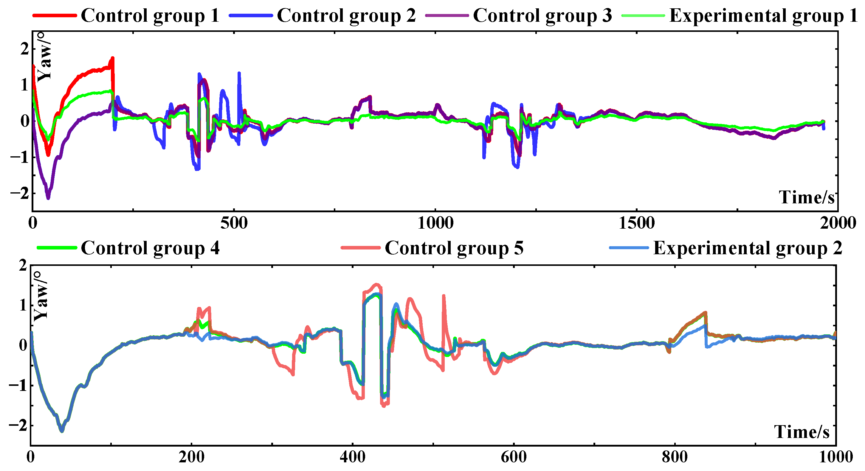
The heading-angle estimation error of the whole test is shown in Figure 13, and the maximum error and the root mean square error are shown in

Table 16. Heading-angle estimation error statistics.

Heading Angle/°	➀	➁	➂	➃	Maximum Improvement	➄	➅	➆	Maximum Improvement
RMS	0.23	0.38	0.42	0.43	46.5%	0.49	0.50	0.57	14.1%
MAX	0.85	1.75	2.14	2.14	60.3%	2.14	2.13	2.14

. As shown in the upper figure in Figure 12, before the first turning time point of 193 s, the heading angles of each group slowly diverge, and the divergence degree of control groups 2 and 3 is relatively large, reaching about 2.3°. At the other turning points, the heading-angle error of each group is affected by road conditions and GNSS signals, and the gross errors are obvious. However, to a certain extent, the adaptive Kalman filter based on a Gaussian–Student’s T mixed distribution exhibits the greatest improvement ability in terms of heading-angle error compared with other groups in special road sections. When the road conditions are good, there is not much difference between the groups. As shown in Figure 12, before 193 s, due to the influence of GNSS signals, the performance of experimental group 2 is weakened, with no significant improvement compared with the other groups. However, in the subsequent special sections, it can be seen that its performance improvement is better than that of the control groups.

Based on the above analysis, the NHC noise adaptive adjustment method based on the vehicle motion state and the Ga-St VBAKF algorithm based on the modeling of the NHC side-vector measurement noise can make full and effective use of the NHC observation information, adjust the tightness of the constraints in time in special sections, and improve the redundancy of the adaptive Kalman filter. When a GNSS signal exists, there are large differences in the positioning results of each group in the turning section, indicating that the NHC noise of vehicles in the turning section has time-varying characteristics and does not obey the Gaussian distribution, which is incompatible with the traditional fixed noise matrix. After the GNSS interruption, the results of each group show the same pattern, and the dispersion of error in the results of the experimental group is significantly lower than that of the control group. However, since the combined navigation completely relies on INS recursion and NHC at this time, the positioning error increases, indicating that GNSS signal interruption reduces the performance of the algorithm to a certain extent. According to the measured data processing results, the GNSS/NHC/OD/INS integrated algorithm based on the Gaussian–Student’s T mixed distribution adaptive Kalman filter can effectively improve the positioning accuracy of the vehicle navigation system in special road sections including turning, sideslip, and bumps. In five 300 s turning sections and a variety of complex scenes, the maximum horizontal position error is reduced by 65.9% near the time point of NHC failure. After the GNSS signal is interrupted in the special road section, the horizontal position error is reduced by 42.3%, at most.

6. Conclusions

During the effective period of the GNSS signal, the NHC and GNSS observations fail, to a certain extent, when the vehicle is turning, sideslipping, or moving up and down. The NHC lateral noise adaptive setting is used to adjust the tightness of NHCs, and the Ga-St VBAKF algorithm based on noise modeling is used to assist GNSS/INS integrated navigation to reduce the positioning error caused by the failure of NHC or GNSS observations. During GNSS signal interruption, the NHC/OD/INS system can effectively suppress the divergence of the integrated navigation and positioning results. On this basis, taking full advantage of the lateral noise characteristics of NHCs, the adaptive adjustment method of NHC noise and the Ga-St VBAKF algorithm can effectively reduce the positioning error and improve the performance of NHCs. The experimental results show that the maximum horizontal position error of the noise-adaptive Ga-St VBAKF algorithm in the GNSS/NHC/OD/INS system is reduced by 65.9% (compared with the control groups) and the maximum horizontal position error in the NHC/OD/INS system is reduced by 42.3%. At the same time, the Ga-St VBAKF algorithm has the smallest divergence of integrated navigation and positioning errors during GNSS outages, indicating that the algorithm can improve the performance of NHCs.