Hyperspectral Data Can Classify Plant Functional Groups Within New Zealand Hill Farm Pasture

Abstract

Reliable evidence of species composition or habitat distribution is essential to advance pasture management and decision making, including the definition of fertiliser rates for aerial top dressing. This is more difficult in a diverse environment such as New Zealand hill country farms. The simplification of the landscape character using plant functional types and species dominance has proven useful in ecological studies and in modelling grasslands. This study used hyperspectral imagery to map hill country pasture into plant functional groups (PFGs) as a proxy for pasture quality. We validated a farm scale map generated using support vector machines (SVMs), with ground reference data, to an overall accuracy of 88.75%. We discuss how that information can improve on-farm decision making and allow for better coordination with off-farm consultants. This form of farm-wide mapping is also critical for the successful application of variable-rate aerial topdressing technology as input for the allocation of fertiliser rates.

1. Introduction

Remote sensing using hyperspectral data is finding a wide array of applications in agriculture and eco-system monitoring [1,2,3,4]. This move to hyperspectral data is mostly due to the increased utility of the information collected with hundreds of contiguous spectral bands in comparison to the 4–11 bands of multispectral systems. Hyperspectral data have been shown to be useful for identifying species variability [5,6,7] and for species mapping [8,9] in various heterogenous natural grassland environments, although progress has been slow in the commercial application of such data in pasture farming. To our knowledge, hyperspectral mapping techniques have yet to be applied to discern species composition in the heterogenous pasture environments of New Zealand hill country farm landscapes. White et al. [10] concluded that pasture delineation using hyperspectral imagery can enhance the commercial benefits of variable-rate aerial topdressing (VRAT) technology through application accuracy. As such, additional benefit would therefore be gained from the addition of relevant data to define application rates at the same time and increase the cost benefit of the aerial survey.

There are three primary platforms capable of collecting hyperspectral imagery, with associated advantages and disadvantages. Satellites can cover vast areas at the cost of spatial and spectral resolution. Unmanned Aerial Vehicles (UAVs) collect high spatial and spectral resolution data but are limited in coverage. Aerial systems (flown in manned aircraft) fit the space between the two with the ability to scan thousands of hectares in a single mission, at excellent spectral and spatial resolutions. Additionally, a survey using aircraft is more easily rescheduled than satellites if conditions overhead are unfavourable, which is often the case in New Zealand.

The landscape that New Zealand’s sheep and beef farms typically occupy is often steep and highly variable, making them less suitable for conversion to higher-value enterprises. These “Hill Country Farms” are often inaccessible by ground transport, so operations such as chemical or fertiliser application must be applied via aircraft, and traditional pasture renewal is often impossible.

The species composition of pasture has a major effect on farm productivity as measured by animal performance [11,12]. The grass preference for both palatability and animal weight gain on New Zealand hill country farms are modern perennial ryegrass cultivars. However, the invasion of weeds and less nutritious species such as browntop (Agrostis capillaris) into new pastures lessens pasture productivity, as measured by animal live weight gain [12]. Stock management, chemical topping, pasture renewal, and fertiliser application are some of the current tools available to farm managers to meet internal and external production goals [13]. Pasture composition and production are linked to farm economic performance and environmental sustainability, as pasture responds to biophysical resources such as soil moisture, soil fertility, and erosion [14]; thus, pasture species in these low-input grass ecologies are heavily influenced by the extreme variability of the landscape [15], making them difficult to predict as they change rapidly, temporally, and spatially [16]. Greater understanding of the relationships between soil, pasture, and environmental factors improves management decisions, provides guidance for fertiliser applications, and protects the environment.

Some species such as ryegrass respond well to higher fertility conditions whilst browntop, for example, although less well adapted to high fertility, can be highly competitive with white clover in the uptake of phosphate [17]. Thus, it would be useful to include habitat and species information when selecting fertiliser application rates. If pasture species composition were known, fertiliser application rates and many other farm decisions could be adjusted to maximise production. For example, the farmer might decide to increase soil fertility and encourage competition by desirable species or to capitalise on existing dominance to increase pasture production without wasting resources on less productive areas. Accurate species information could inform decisions on stocking rates, and pasture quality information would also be relevant to rural property valuations.

Researchers have studied the dynamics of grassland species flux since the 1850s [18]. The species distribution models currently employed are usually based on relationships with spatial and physical characteristics of the landscape and environmental interactions [19]. Unfortunately, many plant–environment relationships are still poorly understood in the complex hill country environment, limiting progress and the accuracy of resulting models in all but localised areas [14].

Grouping plants adapted to similar environments provides insights from the resulting generalisations [20,21,22], and the continued evolution of the discipline promises to expand the utility of the technique, although they have mostly been applied at a regional scale [23,24]. Such categorization of species along fertility and nutrition gradients has proven useful in explaining species composition and productive variability in pasture [25,26]. Grouping species into high-fertility-responsive (HFR) and low-fertility-tolerant (LFT) plant functional groups (PFGs) has been used to describe pasture and to relate environmental factors to their presence [14,27,28]. A few plants usually dominate species composition in New Zealand hill country pastures, with more than half of the available biomass at any location usually comprising three or fewer species. Wan et al. [29] simplified these complex interactions by focusing on three species to identify variables that can influence management. Their research showed that the competitiveness of perennial ryegrass (Lolium perenne) versus browntop could be partially explained by soil Olsen P and slope influence.

Often found on dry hill country soils, browntop tolerates a wide range of growing conditions. Ryegrass is more competitive than browntop in moist, fertile soils, and both species are common throughout New Zealand [30]. Browntop and ryegrass belong to different plant functional groups, CSR and CR/CSR, respectively, as defined by the Grimes C-S-R ecological community triangle [31]. The aim of understanding these environments is to improve production for better farm returns. The New Zealand Government’s policy to increase production [32] coupled with an increased awareness of environmental sustainability [14] are also key factors driving this research. We hypothesise that hyperspectral data could be used to classify hill farm pasture into high- and low-fertility PFGs. This has potential to inform many of the on-farm strategic decision-making processes and possibly lead to new insights into pasture-versus-environment interactions.

Hyperspectral data have been used to describe pasture or grassland quality [24,33], but generating a pasture classification map or species distribution map is uncommon, and when it is carried out it is either at a local scale < 10 ha [8] or at a regional scale using multispectral satellite data [34,35].

To summarise, the problem is the lack of pasture quality information for aiding farm decision making, which is critical for productivity. The landscape is difficult, and species are highly variable. PFGs have been shown to be capable of distilling the fine-scale details of species distribution while maintaining relevance. When coupled with remote sensing, it can allow for the characterisation of pasture quality across large areas such as farm landscapes. Understanding the distribution of pasture quality would help decision making relating to key agricultural issues of pasture management, stock management, pasture renewal, and rural valuation.

The goal of this research was to develop and validate a simple technique to map pasture quality via PFGs using hyperspectral data and support vector machines (SVMs) at the farm scale. This work is a step towards agricultural extension, joining remote sensing with the agricultural consultant community by using off-the-shelf software requiring little or no programming skills. The spatial distribution, at the farm scale, of species previously identified as key indicators of pasture condition, i.e., ryegrass, browntop, and/or legumes such as clover (Trifolium sp.), were defined as PFGs [14,15,22,27,29,36,37,38]. In this study, three PFGs were defined to represent the abundance and dominance of the species. The distribution of these components is also an important component in the definition of fertiliser application rates to better utilise modern VRAT technologies [10] and add to the cost benefit of the aerial survey.

The main contributions from this study are as follows:

• This study used off-the-shelf software and methods to map pasture PFGs to a 1 m² spatial resolution across a 2600 ha farm landscape, showing that complicated methods are not necessary to gain utility from these data.
• The resulting map was validated across 76 ha to provide farming and extension practitioners confidence in results and to encourage its adoption in farming extension endeavours.

2. Materials and Methods

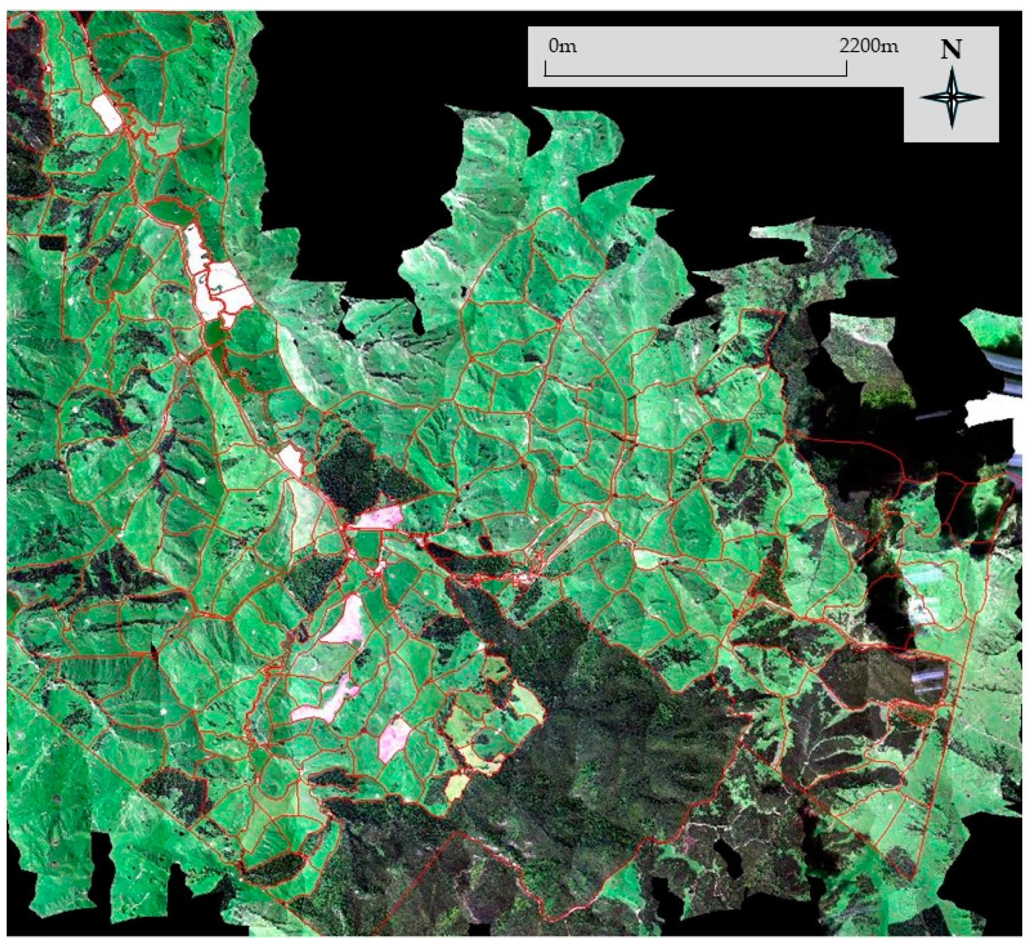
Three primary groups of pasture species, low-fertility-tolerant, high-fertility-responsive, and legumes were defined from on-site species surveys. Hyperspectral data in conjunction with support vector machines were used to train a classification model. The validation of the results was carried out firstly by splitting off a proportion of the ground data collected, adding additional larger areas to the validation from on-site assessments, and lastly by seeking the opinion of the primary expert on the land, the farm owner.

2.1. Site Location

The study was conducted on Patitapu Station in the Wairarapa region on the North Island of New Zealand. This 2617-hectare property has around 1800 hectares of pasture that supports almost 17,000 stock units, with a further 450 hectares of native bush. The terrain ranges from 150 to 534 metres above mean sea level with an annual rainfall of between 800 mm and 1200 mm. Figure 1 provides an aerial view of the property.

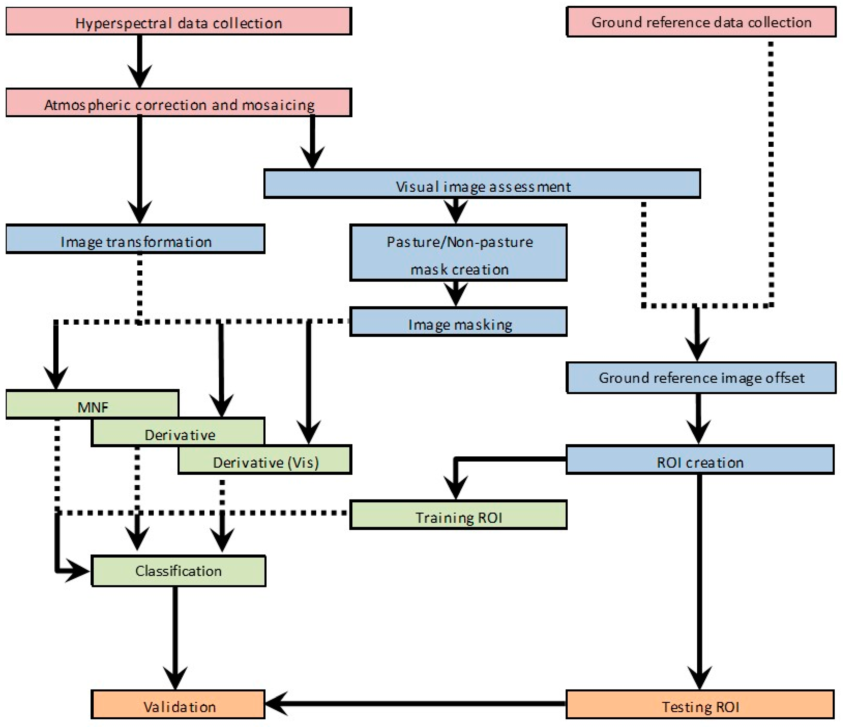
2.2. Method Overview

Figure 2 summarises the workflow for the classification of the hyperspectral imagery. Ground data collected from tarpaulin sites within two days of the aerial survey were used to define regions of interest (ROIs). These were used to train and test the classification. The classification and validation had three stages:

• A combination of hyperspectral imagery and surveyed ground data is used to classify the pasture into three classes representing HFR (ryegrass), LFT (browntop), and legumes (clover) in a method similar to that used by Lambert et al. [27].
• Information was collected on homogeneous paddocks to expand the validation of the original classification and provide greater confidence in the results.
• Another site visit was made to identify specific features visible in the classification results; the features were cross-checked and discussed with the farm manager and owner to obtain their perspective.

2.2.1. Hyperspectral Aerial Survey

An AisaFENIX hyperspectral sensor made by Specim (Finland), was used to obtain aerial imagery of Patitapu Station (Figure 1), beginning at 11.30 a.m. on 2 March 2017. The hyperspectral data covered the range from 380 nm to 2500 nm in 448 spectral bands. They were atmospherically corrected and mosaicked into a single orthorectified image by the Ministry of Primary Industry/Ravensdown Primary Growth Partnership (PGP) team as per Pullanagari et al. [39].

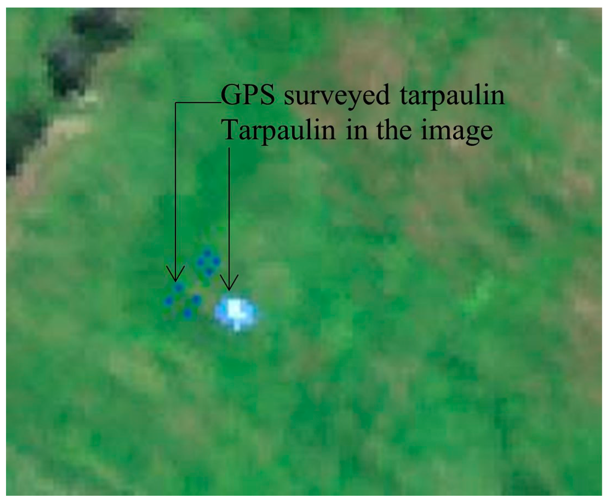
2.2.2. Ground Data Collection (Tarpaulin Sites) Class Assignment

The field survey included visual references (blue 3 m × 3 m blue plastic tarpaulins) large enough to appear in the survey image. Each survey site was positioned 5 m north of a tarpaulin, with both the site and tarpaulin geo-located using a real-time kinematic (RTK) DGPS system; this confirmed the actual site locations and allowed for the positional error in the mosaicked hyperspectral image to be ascertained and a correction to be applied to each location.

Botanical composition data were collected using a 0.9 m × 0.9 m (0.81 m²) quadrat, segmented using elasticated cord into 36 equal sections representing 2.77% each. The quadrat was randomly dropped into the 2 m × 2 m sample site. The percentage of cover was estimated for browntop, ryegrass, clover, dead material, and other pasture components. Other pasture components included broad-leaved weeds and other grass species. Two agronomists performed the visual assessment together to reduce the possibility of bias or estimate drift [40].

The species composition data were converted into a mutually exclusive class of HFR, LFT, or legumes to enable classification. Each site was assigned a user-defined class based on the content (%) of each of the indicator species before data segmentation, into training and test groups. LFT sites were defined as having a greater coverage of browntop, HFR sites were defined with a greater coverage of ryegrass, and the legume class was defined by sites where legumes (clover) were dominant—that is, greater coverage than either ryegrass or browntop. The classification and subsequent validation assume these defined classes are correct. Assignment into mutually exclusive classes reduced the resolution of the ground data collected to 1 m².

2.2.3. Ground Data Collection (Paddock Sites)

It is important that the validation of the classification includes as much of the farm as possible to increase confidence in the results. Given the difficulty and expense associated with surveying individual point locations, homogeneous paddocks represent the best opportunity to collect larger sample areas to validate the resulting classification.

In collaboration with the farm owner, operator experience, and site photography [41] a series of paddocks were identified for inclusion as additional validation. These had ‘relatively’ uniform composition as they were recently renewed (primarily flat paddocks) or because they had a stable browntop-dominated population. These areas were visited and marked on a farm map and had clear paddock boundaries. The paddock boundaries were overlaid on an aerial photograph that facilitated paddock location and identification. The paddock data were held separately and only used for additional validation of the primary classification; i.e., they were not used to train the classifier.

2.2.4. Non-Pasture Masking

It is not always helpful to include the entire scene in an analysis, especially when the scene is complex [42]. Masking is a useful form of data reduction, and, given the focus on pasture in this study, it constrains the classification to only the pasture component. This mask was defined using ENVI software v4.8 (Exelis Visual Information Solutions, Boulder, CO, USA) that involves the collection of pasture and non-pasture ROI before applying a linear support vector machine (SVM) classification; thus, non-pasture components are discarded from the image and excluded from analyses.

2.2.5. Image Transformation

Two forms of data transformation, minimum noise fraction (MNF) and calculation of first derivative, were applied to the data. MNF is similar to a principal component analysis (PCA) that rotates the data to form new variables. The MNF carries most of the useful information in the first few components and the noise in the latter components [43]; 10 transformed components from the MNF were included in the analysis. Transformation to the 1st derivative defines the rate of change from one wavelength to the next and can help reduce low-frequency noise [44]. A dataset was also created that truncates reflectance at 970 nm, which removes the SWIR, as well as a portion of the near infra-red (NIR); 970 nm was used as the cut-off point because it is the point where the two detectors within the AisaFENIX sensor meet [45]. Those sensors have slightly different specifications, including signal-to-noise ratios. The ability to carry out the analysis with a less costly system, one that did not include the SWIR, could have several operational benefits.

2.3. SVM Classification

Support vector machines (SVMs) generate an optimal separating hyperplane using training points that lie on the boundary between the classes (support vectors) [46]. The hyperplane is used to define the class of each pixel. SVMs are a supervised classification method that is well established in remote sensing. With ease of operation in mind, a linear SVM was implemented in ENVI to classify the image and validate results. The linear form of SVM was defined by Hsu et al. [47] as Equation (1).

$$K\left(x_i,x_j\right)=x_i^{ T}{x}_j$$

(1)

With the linear SVM, the only tuning parameter is the soft margin constant, which allows for some misclassification to avoid overfitting; this was left at the default 100 within the ENVI software.

2.3.1. SVM Region of Interest Collection

Supervised classification methods require the user to train the method by supplying examples of each class as regions of interest (ROIs). Species diversity data can be a problem for the selection of ROIs for training and test data. For instance, a small training dataset can reduce the accuracy from some methods such as artificial neural network-type classifiers [48]. SVMs are not so constrained, requiring only support vectors to be identified, so fewer training samples are selected that effectively define the classes of interest [49,50,51]. The advantage of using fewer samples for the training dataset is that a relatively large portion of the total dataset remains available for testing the classification accuracy. Training and test data were held separately as suggested by Stehman [52].

Reinke and Jones [53] state that the positional accuracy of remote sensing data is important. In their case, an offset of a few metres would have placed some of their sites in different environmental settings; this was also the case for this study. Ground data collected in the field must be registered to the correct spectral measurements (pixels) in the image to justify assertions made from analysis. Using tarpaulins for this survey allowed for positional inaccuracies to be corrected. When collecting regions of interest, manual adjustment was used to match the ground data locations to the correct pixels in the image using the offset information listed in

Table 1. Details of the botanical composition collected for the 49 tarpaulin sites. “Classification Training” identifies whether the site was used to train the classification. Cells with “T” had trace amounts of the botanical component present but not enough to make 1%. An asterisk * alongside the user-defined class indicates sites where class assignment was “forced” by inclusion of the “other species” in the determination. Offset direction and distance detail the specific discrepancy between image and GPS site locations.

Inclusion in Classification Training Group	Point ID	Browntop %	Ryegrass %	Clover %	Dead Material %	Other Pasture %	Offset Direction	Offset Distance (m)	User Defined Class
	V1	80	0	10	1	9	65°	3.0	LFT
	V2	77.5	T	2.5	10	10	130°	3.9	LFT
	V3	65	5	20	T	10	110°	8.4	LFT
Y	V4	85	0	T	5	10	110°	8.4	LFT
Y	V5	T	70	25	0	5	110°	6.5	HFR
Y	V6	50	5	0	2	43	135°	3.1	LFT
Y	V7	90	0	T	5	5	130°	4.0	LFT
	V8	35	35	20	5	5	270°	1.0	HFR *
Y	V9	80	0	15	5	0	60°	0.8	LFT
	V10	75	5	10	5	5	110°	5.9	LFT
	V11	20	55	20	2	3	50°	3.6	HFR
	V12	20	40	20	2	18	80°	4.8	HFR
	V13	25	15	25	T	35	105°	11.1	LFT *
	V14	25	0	60	T	35	295°	3.5	L
	V15	10	10	50	T	30	110°	6.7	L
Y	V16	10	5	60	T	25	120°	1.6	L
	V17	20	0	50	T	30	90°	4.3	L
Y	V18	10	5	60	T	25	105°	2.9	L
Y	V19	40	5	10	2	33	130°	5.5	LFT
Y	V20	58	5	25	2	10	140°	4.1	LFT
	V21	20	20	20	2	38	135°	5.7	LFT *
Y	V22	0	99	T	0	1	205°	2.3	HFR
	V23	5	5	50	T	40	90°	3.5	L
Y	V25	3	5	65	2	25	90°	2.9	L
	V28	10	80	10	0	0	110°	7.0	HFR
Y	V29	0	50	50	T	0	110°	3.7	HFR *
	V30	0	80	15	0	5	100°	0.6	HFR
	V31	5	15	5	T	75	80°	1.7	LFT *
	V32	10	0	0	T	90	110°	6.7	LFT
Y	V33	0	75	25	T	0.1	130°	7.1	HFR
Y	V34	0	0	100	0	0	110°	5.8	L
Y	V35	0	0	95	0	5	90°	2.8	L
Y	V36	0	75	5	1	19	105°	5.6	HFR
Y	V37	0	30	40	T	30	50°	3.8	HFR *
Y	V38	50	30	10	1	9	310°	1.0	LFT
	V39	40	40	5	1	14	110°	3.7	LFT *
Y	V40	40	T	T	15	45	350°	2.3	LFT
	V42	15	20	40	1	24	100°	5.6	HFR
Y	V43	85	5	0	5	5	70°	6.7	LFT
Y	V44	10	50	5	5	30	120°	5.8	HFR
Y	V46	10	85	0.1	T	5	140°	4.0	HFR
	V47	0	60	35	0	5	130°	4.8	HFR
Y	V48	0	90	5	0	5	130°	4.9	HFR
	V49	5	39	40	1	15	110°	6.0	HFR
	V50	5	40	40	T	15	110°	6.5	HFR *
	V52	10	30	2	2	56	135°	3.9	LFT *
	vt2	60	0	5	3	32	140°	2.4	LFT
Y	vt27	T	70	30	T	0	130°	3.8	HFR
	vt3	20	10	10	60	0	45°	4.1	LFT

. The quadrat was randomly dropped within the 2 m × 2 m site area, so a number of pixels were needed to ensure that the quadrat location was represented in the ROI. This meant that either 4 or 9 pixels were collected to ensure a match with the site data.

ROIs for validation were collected from the true colour image prior to classification to avoid operator bias [54]. Another class was created to account for the non-data portions (perimeter) of the image, as previous testing indicated the SVM would classify these non-data areas into the nearest class. Legumes were included as a class because clover was prominent in several locations of the survey, and there were also some paddocks sown with 100% clover, which provided good training sites. Nitrogen fixing plants have been singled out by other authors as deserving of their own category, as they uniquely generate their own nitrogen in the root [55]. Four classes, including a “non-data” class, were defined in total. The sites used to train the classification had higher proportions of the desired species, with low amounts of the other species. In the SVM feature space, these sites were expected to identify appropriate support vectors with fewer training components [49,50].

2.3.2. Farm Pasture Regions of Interest

Farm paddocks, identified as “fairly homogeneous” (in terms of hill farm pasture), were added as additional, large-scale regions of interest. These ROIs were only used for additional validation of the classification generated from the survey site data and not used in model training.

2.4. On-Farm Validation Visit

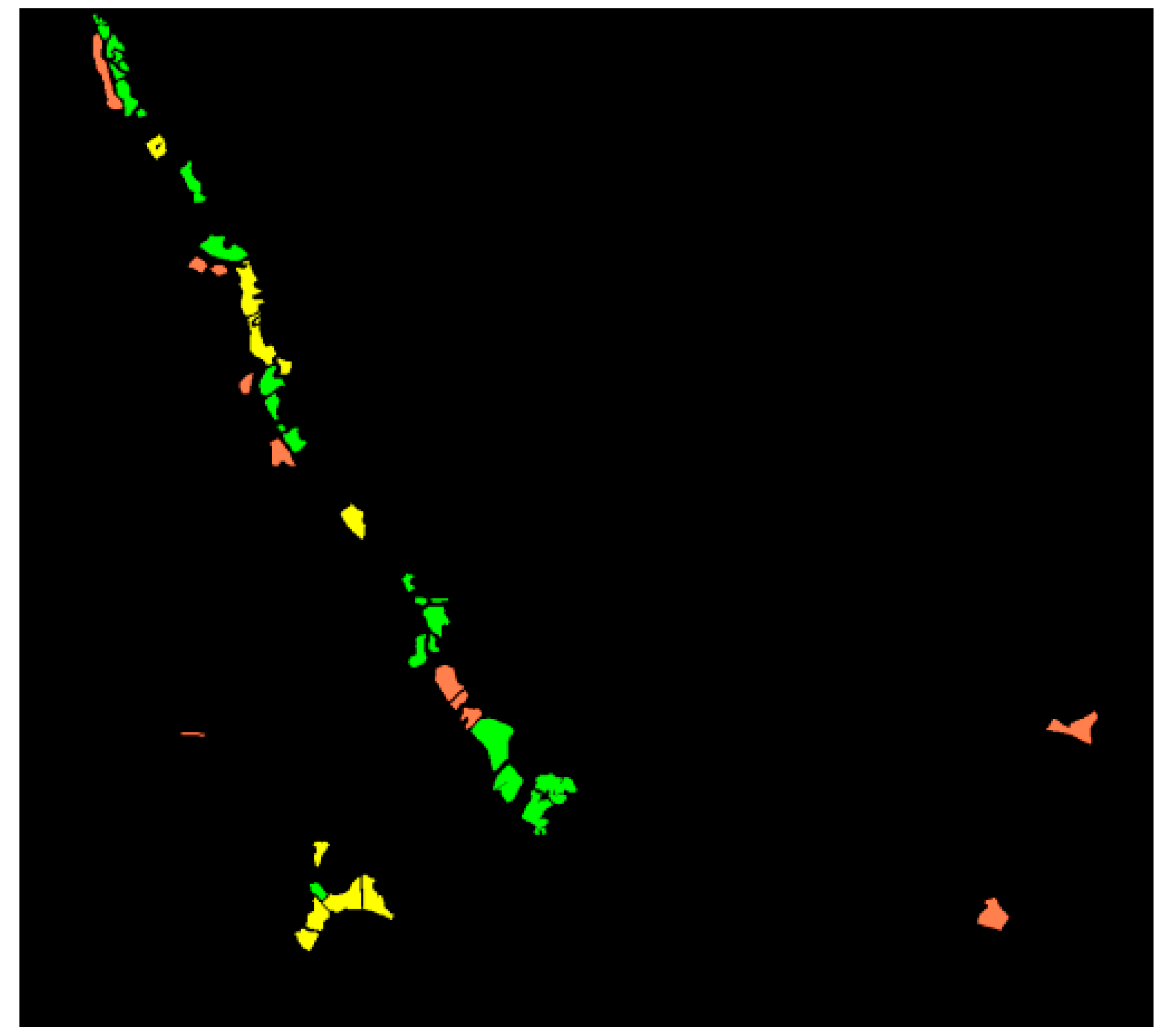
A classification accuracy statistic alone may be too abstract to fully gain the confidence of industry practitioners for whom this work is intended. Therefore, a post-classification visit was conducted to examine prominent landscape features identified from the classification and verify their existence in the landscape.

Five days after the initial ground data collection, an agronomist, accompanied by a farm staff member, toured the farm to assess the general species composition across large areas. The site visit evaluated whether the conditions at the chosen sites matched the classification results.

3. Results

Figure 3a represents the first farm-scale map of pasture composition quality for a New Zealand hill country farm. The map composites in Figure 3 were made up from several survey “strips” that were mosaicked into a single image.

Table 1 lists the user defined category for each survey site; nine sites needed extra consideration before class allocation as none of the primary target species had dominance. For example, site V8 was composed of 35% browntop and 35% ryegrass. In that instance, the high levels of clover (20%) and low levels of other species (5%) allowed this site to be defined as HFR. In contrast, V13 was composed of 25% browntop and 25% clover. Here, the high levels of other species (35%) and low levels of ryegrass (15%) enabled the definition of this site as LFT. Twenty-one of the forty-nine sites were eventually categorised as LFT, ten sites were legume, and eighteen were HFR.

The overall accuracy (OA), assessed using only the ground sample sites, was 56–57%. When paddock ROIs were added to the validation, the accuracy increased to 84–88%. Figure 3a shows the classification of the farm pasture into the various PFGs. Figure 3b is an RGB image of the whole study area as reference.

3.1. Positional Accuracy

Substantial and varied discrepancy between the tarpaulin locations in the imagery and the GPS point data collected in the field was identified through visual interpretation of the hyperspectral image in combination with GPS data. This positional issue was most likely a consequence of the absence of differential GPS correction on board the survey plane, which solely relied on inertial guidance, but the misalignment may also be connected to the poor quality of the digital elevation model (DEM) used in orthorectification (Kereszturi, Personal Communication). This resulted in the GPS points collected in the field not aligning with the specific features in the image (see Figure 4).

Each location was affected differently; in one instance, the measured offset was 11.1 m. Features visible in the image, for example, fence lines and roads, suggest this was not an isolated case. To identify the correct location of the ground survey site in the image, an offset was applied on an individual basis to each location. The direction and distance of the offset was calculated by the difference between the tarpaulin in the image and the GPS points for the tarpaulin.

In two instances, where the sample site was close to the edge of a survey strip, the mosaicking overlapped the tarpaulin with another image strip and “erased” the tarpaulin from the composite image. These sites were eliminated from the analysis, as GPS correction could not be applied. A third site was excluded, as it was erroneously placed outside the property boundary by the setup team, leaving 49 tarpaulin sites available for analysis. Table 1 lists the species composition of each site and the associated positional and directional error recorded between GPS points and image.

3.2. Tarpaulin Site Classification

Table 2. Overall accuracies and associated kappa for each classification with each form of data transformation.

Data Transformation		Tarpaulin Sites	Paddocks
1st Derivative	OA	57.44%	88.75%
	kappa	24.48%	82.72%
MNF	OA	56.02%	86.03%
	Kappa	27.28%	78.11%
1st Derivative	OA	56.02%	84.46%
(No SWIR)	Kappa	14.66%	75.65%

lists the accuracy metrics for each analysis and data type. The OA for the original surveyed locations was consistent (56–57%), regardless of the data type used in the classification. The tarpaulin site accuracy was generated from a subset of 25 sites isolated into the training set. Although the OA was moderate, the kappa statistic did not match as well (14–27%), suggesting poor agreement of class as defined by Monserud and Leemans [56]. The disagreement is due to the very high commission and omission error associated with the legume class. For example, the omission error for the legume class shown in

Table 3. Error types and rates for the 1st derivative data from the tarpaulin sites (OA 57.44%).

Class	Commission	Omission	Commission	Omission
	(%)	(%)	(Pixels)	(Pixels)
LFT	30.49	28.75	25/82	23/80
HFR	59.26	40.54	32/54	15/37
Legume	60	91.67	3/5	22/24

is much higher than other classes; 91% of the pixels defined by the operator as legume are described by the classifier as one of the other classes.

3.3. Classification Validation (Paddock Sites)

Figure 5 shows the class image produced from the ROI of the homogeneous paddocks. The classification was subsequently validated against these additional ROIs.

When the classification was validated against the larger areas of the paddock data, the overall accuracy and kappa both increased markedly to >84% (e.g., Table 2) Data transformation had little effect on the OA again. More importantly, the OA and kappa had much closer agreement, signalling better overall agreement in each class.

The use of kappa statistics as a metric for assessing accuracy was questioned by Foody [57], who suggested “producer” accuracies (100% minus the omission error) as a more useful metric. The “producer” accuracies provide information for each class rather than just a total.

Table 4. Producer accuracies (%) for each classification for paddock validation data with tarpaulin sites included for reference.

	Tarpaulin Sites			Paddock Sites
	1st Der.	MNF	1st Der. (No SWIR)	1st Der	MNF	1st Der. (No SWIR)
LFT	71.25	62.5	80	89.81	64.63	77.7
HFR	59.46	67.57	29.73	84.09	89.06	88.54
Legumes	8.33	16.67	16.67	94.99	99.81	83.71

lists the producer accuracies for each analysis. They often show a large improvement when paddock data are used for comparison of the classification. This was particularly true for the legume class that increased from 8.33% to 94.99% producer accuracy. The full-spectrum, 1st derivative data provided the best overall results when all classes were considered; see Table 2 and Table 4.

3.3.1. On-Farm Validation

The 1st derivative, full-spectrum data were deemed most accurate overall, so they were used in a subsequent site validation visit and in owner discussions. Several pasture classification features were examined. What follows are some of the prominent classification features that were identified and were distinct enough to be visible in the field.

3.3.2. Classification Feature, On-Farm Validation 1

Figure 6 shows a close-up view for one portion of the classification of “Springhill Flat”, and a very distinctive class change from clover to HFR. Physical and topographic constraints limited the extent of the cultivation and sowing. There is a slope leading down from the farm entry road, where a ditch was installed to facilitate surface drainage (photo at point E). The ditch constrained the sowing operation. Assessment of the species on these boundaries by a trained agronomist confirmed the paddock was legumes while the boundary area was dominated by ryegrass. Although GPS data were not collected (and would have been unhelpful with the error in the imagery) the features were closely reflected in the classification. The clear definition of the sown extents of this crop provides strong validation support for the classification accuracy and also provided the farmer with a result he could validate and interpret from his own knowledge of the farm.

3.3.3. Classification Feature, On-Farm Validation 2

Figure 7 shows another region of the farm classification. The images show that species distribution features, which can be visually verified the photographs, are well defined in the classification. In Figure 7, the northern boundary of ‘area 1’ has a steep hill with a drainage ditch at the base. Unlike the rest of the paddock, that hill had not been cultivated nor sown in ryegrass. In discussion with the farm owner, the classification matched well with his understanding of the “real life” situation. The farmer confirmed the LFT classification of area ‘2’, shown in Figure 7, as accurate and described the soil on that hill as “poor”. The site visit and discussion with the farmer support the overall accuracy of the classification.

3.3.4. Classification Feature, On-Farm Validation 3

Two more locations examined for their accuracy are shown in Figure 8. The photograph taken at point ‘I’ highlights the pasture growth produced since the autumn rains started. Although browntop (HFR) was present on both sides of the boundary, ryegrass easily dominated the eastern side (right in photo). The site visit validated the accuracy of the classification.

The return visit to the sample location, Point ‘J’ in ‘Paddock 1’ (Figure 8), confirmed the validity of the ryegrass classification (HFR) for that location despite much of the surrounding area being dominated by browntop (LFT). Point ‘J’ lies atop a hill with the surrounding area having high quantities of ryegrass. Strong slopes radiate down from this site, in particular to the north and west, all of which were assessed at multiple locations as being browntop dominant. A farm worker commented that the top of the hill was a stock camp (location where animals rest, generally flat), and ryegrass is more competitive in high-fertility situations [58] such as stock camps. The flat location and increased nutrient deposition from animal excreta could explain the ability of ryegrass to persist in a largely browntop-dominated region of the farm.

4. Discussion

This study produced the first farm scale map of pasture quality on hill farm pasture. This 1 m² resolution map, across 1800 hectares is a vast improvement on the existing knowledge base which relies on local expert knowledge and unreliable growth models [14]. This provides a major advance in the research relating to hill farm pasture composition and distribution especially given the current lack of spatially referenced pasture data. We were able to generate these results with stock methods in commercially available software which supports our assertion that such tasks can be carried out with a minimal amount of training.

4.1. Remote Sensing

There have been several advances in our understanding of remotely sensed mapping of PFGs in recent years that hold promise to further improve on this work or at least grant us a better understanding of its limitations [59,60,61]. However, further improvement would require a multidisciplined team to integrate our understanding of pasture plant–environment interactions with appropriate remote sensing data. In the meantime, the current work provides access to spatially referenced data that have multiple farm management uses and benefits.

New Zealand hill country pastures are known for their variability [29,37], which is supported by the species composition data in this study. Assigning classes to the ground survey data was challenging for several sites. For example, sample V8 (Table 1) had relatively uniform coverage from all main indicator species, complicating class assignment for training. Classification requires each site to be assigned to a single class. When the distinction is clear, the pixel can be considered a “pure” example for both training and classification purposes. However, in several cases, the distinction was less than ideal, so expert knowledge was used to “force” inclusion into a single exclusive category. Imposing a category when it is not clear can have severe implications for training a classification [49,51].

To mitigate the potential negative effects on classification, sound reasoning was applied in cases where the composition was not ideal. Contributions from other categories guided the class decision in such cases. When a single indicator species was not dominant, other species were combined to define the class. Browntop was combined with the group “other species” into LFT, and ryegrass was combined with legumes into HFR. Ryegrass and clover are commonly sown together to promote a symbiotic partnership [12], so it is reasonable to combine them into the HFR class when ryegrass is present. Contributions from the “other species” group in the pasture was attributed to the LFT class, as the ingress of many other species signals a possible decline in pasture quality [27].

The primary disadvantage of classifying heterogenous species mixtures into a single class is the potential loss of resolution. Where we may have a pixel with five or more species, we end up with a single class to describe them all as a group. This “loss” is only relevant when such species information has greater importance than the resulting class. It is unimportant when the resulting class is adequate for the task. In this case, the 1m spatial resolution map is arguably still too detailed for practical application by the farm manager or rural support services, so keeping further detail is both unnecessary and a potential waste of resources.

4.2. Classifier Performance Assessment

The initial overall accuracy (OA) of 56–57% compares well with that by Josh et al. [59], although they were working with multispectral Sentinel-2 data. The OA for the classification considers the accuracy for all the classes combined. Many in the remote sensing community define the acceptable classification accuracy as >85%, although this target appears to have been adopted without regard to its origin [57]. Foody [57] suggested that a project’s individual objectives should define acceptable classification accuracy, as lower accuracies may still represent a success. Results from the tarpaulin sites did not meet the 85% accuracy target suggested for such maps. There are several possible reasons for the initial poor accuracy metrics other than the potential unsuitability of the analysis. These reasons include the need to collect ROIs from image areas that were much larger than the ground sampling site, positional inaccuracy of the image, the small number of reference locations for both classification or validation, and operator error while collecting ground reference data. These problems are not uncommon; Möckel et al. [6] highlighted similar problems in their study.

The diverse landscape means pasture composition can change over short distances [15]. Due to operational constraints, the number of sample sites was limited, preventing the collection of additional samples. The small ground survey areas and the need to collect ROIs from larger sections within the image than on the survey site contributed to potential classification errors. Given the high variability in pasture, it is likely that species composition changed outside the immediate survey location, introducing potential errors into the classification. Ground reference error is a common challenge when validating remote sensing outputs [62]. Even when classifications achieve high accuracy, the lack of detailed ground reference data from a large number of sample sites makes it difficult to validate in highly variable landscapes [62].

Spatial error in the imagery is another significant source of error, especially in defining training samples for classification. While previous reports indicated that the spatial error of imagery collected with this system was only 2–3 m [39], this study found the actual error to be two to four times greater (i.e., 4 m–12 m). This raised concerns that the validation targets were too small to be relevant for practical farming needs or for mapping pasture quality effectively. To address these issues and compensate for the relatively small sample size, the focus shifted towards on-site validation, using larger targets with known homogeneous pasture content. This approach allowed us to confirm that the classification performed better than initially reported by the system.

4.3. On-Farm Validation Features

This study initially faced the same challenge as others that rely on costly ground data collection to map features [39,63,64], namely the issue of limited sample sizes for both modelling and validation. A key challenge in determining classification accuracy is the need to gather sufficient quantities of appropriate ground reference data, which can be costly to obtain. Sometimes referred to as “ground truth”, the term is often used to describe ground reference data and is criticised for the potential exaggeration implied by the term “truth” [57,65]. Ground reference data points with associated species compositions for this study are listed in Table 1. Almost every site has a unique composition, and while “other” species are not listed, more than 20 species were identified in previous surveys on this farm with other researchers having found over 40 species in hill country pasture [15].

The inclusion of additional paddock validation data significantly increased the proportion of the image assessed for accuracy, from 141 pixels to 766,934 pixels (141 m² to 76.69 hectares), and increased the OA to >84%. This is a critical consideration when presenting results and discussing the validity or practical utility of such an analysis, especially to farm owners or managers. While this increase in validation area does not guarantee that the results extrapolated over the entire 2617-hectare farm are consistent beyond the validated zones, it certainly enhances our confidence in the results compared to the initial 141 m² validation.

4.4. Management Support

The classification developed in this research provides valuable information not currently available. The classification not only provides accurate pasture quality information but can also provide accurate pasture area data to support farmer decision making and increase the return on investment for the aerial survey. Further, this classification can define detail with spatial references so that the farmer can examine the results with a suitable map on a paddock-by-paddock basis without additional interpretation. Such maps could support decision making on ideal stocking rates, identify suitable fence positions, and aid in the allocation of fertiliser resources.

The simplicity and user-friendly nature of the output would be attractive to an industry that, partially because of its remoteness, often has poor access to high-quality Internet and communications infrastructure. In addition, pasture quality information currently only resides with the farmer in the form of expert knowledge, which is difficult to share. Mapping pasture quality using a classification method such as this allows information to be easily exchanged, granting external farming consultants a window into the farm, which could form the basis for an improved advisory service.

4.5. Pasture Growth Model Building

Previous research on the prediction of pasture quality or production concentrated on the use of growth models [12,19,29]. Such models are a great tool to help explain the unknown from a small number of known components but are limited by the quality of the input variables. A possible short-term use for this form of classification is as an input variable for improving the modelling of pasture production, replacing digital elevation models that are not yet accurate enough at the farm scale.

An improved model could create multiple scenarios to generate a risk profile for management decisions. Temporal surveys could be overlaid with management data to model the response to various grazing and fertiliser decisions that could form the basis for updating and individualising the model. A more detailed understanding of what factors are changing the species distribution over time would increase the overall body of knowledge to improve models in other locations. Eventually, the farm model would be a business asset that could transfer to a new owner as part of a sale agreement with the land. A high-quality farm growth model may also increase the value of associated land, especially if the model is accepted or proven to be reliable. This would be a vast improvement over current practice, where the new owner or manager must learn the intricacies of the property for themselves, which currently risks failure and financial uncertainty.

4.6. Implications for Fertility Management

Improving fertiliser application efficiency is central to this research. The ability to deliver products accurately from variable-rate systems is limited in hill country due to inadequacies of the current method for calculating fertiliser rates, as is shown in the simplified diagram in Figure 9. The spatial variability of soil nutrients on hill farms is widely recognised [66]. Collecting samples along a series of transacts remains the best method to supply data for such decision making, and efforts to ensure the methods are as robust as possible have been made [67]. A more advanced, spatially accurate understanding of the pasture will help hill country farmers fully realise the benefits of variable-rate application technology. This research shows that remote sensing technologies can provide a better understanding of the pasture environment, with information that can be integrated into pasture growth models, application maps, and normal day-to-day decision making. An example of how this form of analysis could integrate into the process that defines fertiliser requirements and application is shown in Figure 10.

Figure 9 depicts the current knowledge inputs that are associated with the blanket application of fertilisers as the current standard practice.

Figure 10 depicts how the increased and improved information might be integrated into a new solution for the allocation of fertiliser rates, as well as provide maps for automated application technologies.

4.7. Accessibility of Data

The ability of farmers and others to access the type of data used in this study is currently problematic due to the limited availability of aerial imaging systems and survey capable aircraft. The Ravensdown fertiliser company, who developed variable-rate aerial topdressing technology [68] are, on the surface, an obvious group who might implement such surveys as a service and to complement their own technology. However, a more likely scenario is that an independent survey provider offers the service and analysis for a fee.

Another possible avenue for data collection, which would overcome slow data collection from aerial systems, is to use satellite data. This will become more widespread when hyperspectral satellite technology becomes more readily available, at a suitable price point, as well as at suitable spatial and spectral resolutions. A number of hyperspectral satellites are in development or already in orbit [69], so this option could possibly meet the demand in the near future. Of course, a comparative analysis would be required to confirm it has similar or “good enough” utility in comparison to aerial imagery and would be a great follow-up study to this work.

5. Conclusions

The most important finding of this work confirms that the distribution of key, pasture indicator species can be mapped at accuracy levels, where their use would be of benefit in practical on-farm decision making.

This work managed this task in a heterogenous environment using hyperspectral data, and we showed that this system can provide usable farm scale maps. We also showed that this can act as a proxy to map farm pasture quality and habitat without collecting vast amounts of ground reference data.

It is suggested that this classification system can effectively inform operational and management decisions. For this use, it is crucial that the classification accurately reflect ground conditions as recognised by the farm manager, which is even more important than statistical accuracies, as they can be greatly impacted by ground reference data. Therefore, we believe industry professionals can trust the decisions made based on this information.

Including larger homogeneous areas in data collection will almost certainly improve the accuracy, and future work should build on this to further improve results and confidence in them. At this stage, classifications, such as this, are the only method that can be used to economically collect data that are relevant for use with variable-rate aerial topdressing technology. As such, this may provide a financial incentive to streamline or improve the output. Future research should also consider using satellite data, as they are more likely to meet the demand at farm and regional scales.

References

1. Sanches, I.D.A. Hyperspectral Proximal Sensing of the Botanical Composition and Nutrient Content of New Zealand Pastures. Ph.D. Thesis, Massey University, Palmerston North, New Zealand, 2009. [Google Scholar]
2. Sobhan, M.I. Species Discrimination from a Hyperspectral Perspective; Wageningen University and Research: Wageningen, The Netherlands, 2007. [Google Scholar]
3. Thulin, S. Hyperspectral Remote Sensing of Temperate Pasture Quality. Ph.D. Thesis, RMIT University, Melbourne, VIC, Australia, 2008. [Google Scholar]
4. Park, B.; Lu, R. Hyperspectral Imaging Technology in Food and Agriculture; Food engineering series; Springer: New York, NY, USA, 2015. [Google Scholar]
5. Möckel, T. Hyperspectral and Multispectral Remote Sensing for Mapping Grassland Vegetation; Department of Physical Geography and Ecosystem Science, Lund University: Lund, Sweden, 2015. [Google Scholar]
6. Möckel, T.; Dalmayne, J.; Schmid, B.; Prentice, H.; Hall, K. Airborne Hyperspectral Data Predict Fine-Scale Plant Species Diversity in Grazed Dry Grasslands. Remote Sens. 2016, 8, 133. [Google Scholar] [CrossRef]
7. Peng, Y.; Fan, M.; Bai, L.; Sang, W.; Feng, J.; Zhao, Z.; Tao, Z. Identification of the best hyperspectral indices in estimating plant species richness in sandy grasslands. Remote Sens. 2019, 11, 588. [Google Scholar] [CrossRef]
8. Zhu, X.; Bi, Y.; Du, J.; Gao, X.; Zhang, T.; Pi, W.; Zhang, Y.; Wang, Y.; Zhang, H. Research on deep learning method recognition and a classification model of grassland grass species based on unmanned aerial vehicle hyperspectral remote sensing. Grassl. Sci. 2023, 69, 3–11. [Google Scholar] [CrossRef]
9. Marcinkowska-Ochtyra, A.; Jarocińska, A.; Bzdȩga, K.; Tokarska-Guzik, B. Classification of expansive grassland species in different growth stages based on hyperspectral and LiDAR data. Remote Sens. 2018, 10, 2019. [Google Scholar] [CrossRef]
10. White, M.D.; Metherell, A.K.; Roberts, A.H.C.; Meyer, R.E.; Cushnahan, T.A. Economics of a variable rate fertiliser strategy on a Whanganui hill country station. J. N. Z. Grassl. 2017, 79, 125–129. [Google Scholar] [CrossRef]
11. Sanderson, K.; Webster, M. Economic Analysis of the Value of Pasture to the New Zealand Economy; Report to Pasture Renewal Charitable Trust; BERL: Wellington, New Zealand, 2009; p. 42. [Google Scholar]
12. Barenbrug NZ Ltd.; Pasture Renewal Charitable Trust (PRCT). Encouraging Farmers to Renew 10% of Pasture Annually. Barenbrug NZ Ltd. Available online: https://www.barenbrug.co.nz/news/pasture-renewal-charitable-trust-(prct)-encouraging-farmers-to-renew-10-of-pasture-annually.htm (accessed on 15 November 2024).
13. Lambert, M.G.; Clark, D.; Litherland, A. Advances in pasture management for animal productivity and health. N. Z. Vet. J. 2004, 52, 311–319. [Google Scholar] [CrossRef]
14. Lambert, M.G.; Barker, D.J.; Mackay, A.D.; Springett, J. Biophysical indicators of sustainabillty of North Island hill pasture systems. In Proceedings of the Conference-New Zealand Grassland Association, Waitangi, New Zealand, 4–7 March 1996. [Google Scholar]
15. López, I.F.; Valentine, I.; Lambert, M.G.; Hedderley, D.I.; Kemp, P.D. Plant functional groups in a heterogeneous environment. N. Z. J. Agric. Res. 2006, 49, 439–450. [Google Scholar] [CrossRef]
16. Kemp, P. (Massey University, Palmerston North, New Zealand). Personal Communication, 2017.
17. Jackman, R.; Mouat, M. Browntop and pasture nutrition. In Proceedings of the Conference New Zealand Grassland Association, Oamaru, New Zealand, 17–20 October 1994. [Google Scholar]
18. Hill, M.; Carey, P. Prediction of yield in the Rothamsted Park Grass Experiment by Ellenberg indicator values. J. Veg. Sci. 1997, 8, 579–586. [Google Scholar] [CrossRef]
19. Zhang, B.; Valentine, I.; Kemp, P. Modelling the productivity of naturalised pasture in the North Island, New Zealand: A decision tree approach. Ecol. Model. 2005, 186, 299–311. [Google Scholar] [CrossRef]
20. Grime, J.P. Plant Strategies and Vegetation Processes; John Wiley and Sons: Hoboken, NJ, USA, 1979. [Google Scholar]
21. Ellenberg, H. Vegetation Ecology of Central Europe; Cambridge University Press: Cambridge, UK, 1988. [Google Scholar]
22. Grime, J.P. Vegetation classification by reference to strategies. Nature 1974, 250, 26–31. [Google Scholar] [CrossRef]
23. Calbi, M.; Boenisch, G.; Boulangeat, I.; Bunker, D.; Catford, J.A.; Changenet, A.; Culshaw, V.; Dias, A.S.; Hauck, T.; Joschinski, J.; et al. A novel framework to generate plant functional groups for ecological modelling. Ecol. Indic. 2024, 166, 112370. [Google Scholar]
24. Roberts, C.P.; Naugle, D.E.; Allred, B.W.; Donovan, V.M.; Fogarty, D.T.; Jones, M.O.; Maestas, J.D.; Olsen, A.C.; Twidwell, D. Next-generation technologies unlock new possibilities to track rangeland productivity and quantify multi-scale conservation outcomes. J. Environ. Manag. 2022, 324, 116359. [Google Scholar]
25. Shoko, C.; Mutanga, O.; Dube, T. Progress in the remote sensing of C3 and C4 grass species aboveground biomass over time and space. ISPRS J. Photogramm. Remote Sens. 2016, 120, 13–24. [Google Scholar]
26. Boer, M.; Stafford Smith, M.; Lepš, J. A plant functional approach to the prediction of changes in Australian rangeland vegetation under grazing and fire. J. Veg. Sci. 2003, 14, 333–344. [Google Scholar]
27. Lambert, M.G.; Clark, D.A.; Grant, D.A.; Costall, D.A. Influence of fertiliser and grazing management on North Island moist hill country 2. Pasture botanical composition. N. Z. J. Agric. Res. 1986, 29, 1–10. [Google Scholar]
28. López, I.F. Ecology of Pastoral Communities in a Heterogeneous Environment. Ph.D. Thesis, Massey University, Palmerston North, New Zealand, 2000. [Google Scholar]
29. Wan, L.; Zhang, B.; Kemp, P.; Li, X. Modelling the abundance of three key plant species in New Zealand hill-pasture using a decision tree approach. Ecol. Model. 2009, 220, 1819–1825. [Google Scholar]
30. Lambrechtsen, N.C. What Grass Is That? A Guide to Identification of Some Introduced Grasses in New Zealand by Vegetative Characters. Available online: https://natlib.govt.nz/records/21992996 (accessed on 15 November 2024).
31. Hodgson, J.; Wilson, P.; Hunt, R.; Grime, J.; Thompson, K. Allocating CSR plant functional types: A soft approach to a hard problem. Oikos 1999, 85, 282–294. [Google Scholar] [CrossRef]
32. Ministry of Primary Industries. Pioneering to Precision: Application of fertiliser in Hill Country. Available online: https://www.mpi.govt.nz/funding-rural-support/primary-growth-partnerships-pgps/completed-pgp-programmes/pioneering-to-precision-application-of-fertiliser-in-hill-country/ (accessed on 15 November 2024).
33. Jackman, P.; Lee, T.; French, M.; Sasikumar, J.; O’Byrne, P.; Berry, D.; Lacey, A.; Ross, R. Predicting Key Grassland Characteristics from Hyperspectral Data. AgriEngineering 2021, 3, 313–322. [Google Scholar] [CrossRef]
34. Rapinel, S.; Rossignol, N.; Hubert-Moy, L.; Bouzillé, J.B.; Bonis, A. Mapping grassland plant communities using a fuzzy approach to address floristic and spectral uncertainty. Appl. Veg. Sci. 2018, 21, 678–693. [Google Scholar]
35. Seyler, F.; Chaplot, V.; Muller, F.; Cerri, C.E.P.; Bernoux, M.; Ballester, V.; Feller, C.; Cerri, C.C.C. Pasture mapping by classification of Landsat TM images. Analysis of the spectral behaviour of the pasture class in a real medium-scale environment: The case of the Piracicaba Catchment (12400 km2, Brazil). Int. J. Remote Sens. 2002, 23, 4985–5004. [Google Scholar] [CrossRef]
36. Nicholas, P.K. Environmental and Management Factors as Determinants of Pasture Diversity and Production of North Island, New Zealand Hill Pasture Systems. Ph.D. Thesis, Pastures and Crops Group, Institute of Natural Resources, Massey University, Palmerston North, New Zealand, 1999. [Google Scholar]
37. Kemp, P.; Lopez, I. Hill country pastures in the southern North Island of New Zealand: An overview. Hill Country Symposium. Grassland Research and Practice. Thom, R., Ed.; 2016, pp. 289–297. Available online: https://www.nzgajournal.org.nz/index.php/rps/article/view/3241 (accessed on 15 November 2024).
38. Schmidtlein, S.; Tichý, L.; Feilhauer, H.; Faude, U. A brute-force approach to vegetation classification. J. Veg. Sci. 2010, 21, 1162–1171. [Google Scholar]
39. Pullanagari, R.R.; Kereszturi, G.; Yule, I.J. Mapping of macro and micro nutrients of mixed pastures using airborne AisaFENIX hyperspectral imagery. ISPRS J. Photogramm. Remote Sens. 2016, 117, 1–10. [Google Scholar]
40. Bacaro, G.; Baragatti, E.; Chiarucci, A. Using taxonomic data to assess and monitor biodiversity: Are the tribes still fighting? J. Environ. Monit. 2009, 11, 798–801. [Google Scholar] [PubMed]
41. Gienko, G.; Govorov, M. Improving the efficiency of image interpretation using ground truth terrestrial photographs. In Remote Sensing Techniques and GIS Applications in Earth and Environmental Studies; Santra, A., Mitra, S.S., Eds.; IGI Global: Hershey, PA, USA, 2017; p. 39. [Google Scholar]
42. Boardman, J.W.; Kruse, F.A.; Green, R.O. Mapping Target Signatures via Partial Unmixing of AVIRIS Data, N95-33737. 1995. Available online: https://ntrs.nasa.gov/api/citations/19950027316/downloads/19950027316.pdf (accessed on 15 November 2024).
43. Green, A.A.; Berman, M.; Switzer, P.; Craig, M.D. A transformation for ordering multispectral data in terms of image quality with implications for noise removal. IEEE Trans. Geosci. Remote Sens. 1988, 26, 65–74. [Google Scholar]
44. Demetriades-Shah, T.H.; Steven, M.D.; Clark, J.A. High resolution derivative spectra in remote sensing. Remote Sens. Environ. 1990, 33, 55–64. [Google Scholar]
45. SPECIM. AsiaFENIX VNIR/SWIR Hyperspectral Imager User Manual Ver. 1.7; SPECIM, S.I.L.: Oulu, Finland, 2013. [Google Scholar]
46. Ben-Hur, A.; Weston, J. A user’s guide to support vector machines. In Data Mining Techniques for the Life Sciences; Carugo, O., Eisenhaber, F., Eds.; Humana: Totowa, NJ, USA, 2010; pp. 223–239. [Google Scholar] [CrossRef]
47. Hsu, C.-W.; Chang, C.-C.; Lin, C.-J. A Practical Guide to Support Vector Classification; National Taiwan University. 2003. Available online: https://www.datascienceassn.org/sites/default/files/Practical%20Guide%20to%20Support%20Vector%20Classification.pdf (accessed on 15 November 2024).
48. Foody, G.M.; Arora, M. An evaluation of some factors affecting the accuracy of classification by an artificial neural network. Int. J. Remote Sens. 1997, 18, 799–810. [Google Scholar]
49. Foody, G.M.; Mathur, A. Toward intelligent training of supervised image classifications: Directing training data acquisition for SVM classification. Remote Sens. Environ. 2004, 93, 107–117. [Google Scholar]
50. Foody, G.M.; Mathur, A. The use of small training sets containing mixed pixels for accurate hard image classification: Training on mixed spectral responses for classification by a SVM. Remote Sens. Environ. 2006, 103, 179–189. [Google Scholar]
51. Foody, G.M.; Mathur, A.; Sanchez-Hernandez, C.; Boyd, D.S. Training set size requirements for the classification of a specific class. Remote Sens. Environ. 2006, 104, 1–14. [Google Scholar]
52. Stehman, S.V. Sampling designs for accuracy assessment of land cover. Int. J. Remote Sens. 2009, 30, 5243–5272. [Google Scholar]
53. Reinke, K.; Jones, S. Integrating vegetation field surveys with remotely sensed data. Ecol. Manag. Restor. 2006, 7, S18–S23. [Google Scholar]
54. Stehman, S.; Wickham, J.; Smith, J.; Yang, L. Thematic accuracy of the 1992 National Land-Cover Data for the eastern United States: Statistical methodology and regional results. Remote Sens. Environ. 2003, 86, 500–516. [Google Scholar]
55. Asner, G.P.; Jones, M.O.; Martin, R.E.; Knapp, D.E.; Hughes, R.F. Remote sensing of native and invasive species in Hawaiian forests. Remote Sens. Environ. 2008, 112, 1912–1926. [Google Scholar]
56. Monserud, R.A.; Leemans, R. Comparing global vegetation maps with the Kappa statistic. Ecol. Model. 1992, 62, 275–293. [Google Scholar]
57. Foody, G.M. Harshness in image classification accuracy assessment. Int. J. Remote Sens. 2008, 29, 3137–3158. [Google Scholar]
58. Matthew, C.; Tillman, R.W.; Hedley, M.J.; Thompson, M.C. Observations on the relationship betweensoil fertility, botanical composition and pasture growth rate; for a north island lowland pasture. Proc. N. Z. Grassl. Assoc. 1988, 49, 4. [Google Scholar]
59. Josh, E.; Caughlin, T.T.; Hamid, D.; Nancy, F.G. Applied soft classes and fuzzy confusion in a patchwork semi-arid ecosystem: Stitching together classification techniques to preserve ecologically-meaningful information. Remote Sens. Environ. 2023, 300, 113853. [Google Scholar]
60. Anna, K.S.; Anna, K.S.; Martin, S.; Martin, S.; Anita, C.R.; Anita, C.R.; Mathias, K.; Mathias, K.; Rudolf, H.; Rudolf, H.; et al. How to predict plant functional types using imaging spectroscopy: Linking vegetation community traits, plant functional types and spectral response. Methods Ecol. Evol. 2017, 8, 86–95. [Google Scholar]
61. Suvarna, P.; Survarna, P.; Anne, V.; Anne, V.; Irina, T.; Irina, V.T.; Christiaan van der, T.; Christiaan van der, T.; David, M.; David, M.; et al. Characterization of a Highly Biodiverse Floodplain Meadow Using Hyperspectral Remote Sensing within a Plant Functional Trait Framework. Remote Sens. 2016, 8, 112. [Google Scholar] [CrossRef]
62. Foody, G.M. Assessing the accuracy of land cover change with imperfect ground reference data. Remote Sens. Environ. 2010, 114, 2271–2285. [Google Scholar]
63. Fernández-Habas, J.; Carriere Cañada, M.; García Moreno, A.M.; Leal-Murillo, J.R.; González-Dugo, M.P.; Abellanas Oar, B.; Gómez-Giráldez, P.J.; Fernández-Rebollo, P. Estimating pasture quality of Mediterranean grasslands using hyperspectral narrow bands from field spectroscopy by Random Forest and PLS regressions. Comput. Electron. Agric. 2022, 192, 106614. [Google Scholar]
64. Oldeland, J.; Dorigo, W.; Lieckfeld, L.; Lucieer, A.; Jürgens, N. Combining vegetation indices, constrained ordination and fuzzy classification for mapping semi-natural vegetation units from hyperspectral imagery. Remote Sens. Environ. 2010, 114, 1155–1166. [Google Scholar]
65. Brogaard, S.; Ólafsdóttir, R. Ground-truths or Ground-lies?: Environmental sampling for remote sensing application exemplified by vegetation cover data. In Lund Electronic Reports in Physical Geography; Department of Physical Geography, Lund University: Lund, Sweden, 1997; Volume 1. [Google Scholar]
66. During, C.; Mountier, N. Sources of error in advisory soil tests: III. Spatial variance. N. Z. J. Agric. Res. 1967, 10, 134–138. [Google Scholar]
67. Morton, J.; Baird, D.; Manning, M. A soil sampling protocol to minimise the spatial variability in soil test values in New Zealand hill country. N. Z. J. Agric. Res. 2000, 43, 367–375. [Google Scholar]
68. Murray, R.I. Variable Rate Application Technology in the New Zealand Aerial Topdressing Industry. Ph.D. Thesis, Massey University, Palmerston North, New Zealand, 2007. [Google Scholar]
69. Qian, S.E. Hyperspectral Satellites, Evolution, and Development History. IEEE J. Sel. Top. Appl. Earth Obs. Remote Sens. 2021, 14, 7032–7056. [Google Scholar]
Figure 1. Aerial RGB image of Patitapu Station produced from AisaFENIX hyperspectral data. Farm and paddock boundaries are in red.
Remotesensing 17 01120 g001
Figure 2. Simplified workflow diagram of the steps taken for this analysis. Colour coding defines the stages: data collection and automated atmospheric correction (red), image transformation and data preparation (blue), classification (green), and interpretation of results against ground data (orange).
Remotesensing 17 01120 g002
Figure 3. (a) SVM classification of the pasture at Patitapu Station using the 1st derivative data, with green representing HFR, red representing LFT, and yellow representing legumes. (b) Colour image of the study site with paddock boundaries defined by blue lines. Black regions are either missing data or masked out as non-pasture (NP) prior to classification.
Remotesensing 17 01120 g003
Figure 4. View of one site (V12) showing the 4.8 m spatial alignment offset between the image and GPS coordinates collected during the ground survey of the tarpaulin site.
Remotesensing 17 01120 g004
Figure 5. Region of interest image created from on site assessment and with the aid of the farm manager. Green are paddocks seeded with a ryegrass (HFR)-dominated seed mix. Yellow are paddocks sown with 100% legumes (white and red clover). Red are locations where browntop (LFT) dominate the sward in most, or all, of the paddocks.
Remotesensing 17 01120 g005
Figure 6. Classification of “Springhill Flat”, which was sown in legumes (yellow). Photographs were taken at the locations (D and E) in the direction of the arrow. The blue arrows highlight the extent of clover sowing. The sowing was visible from point ‘E’, which is constrained by a drainage ditch. Green = HFR, yellow = legumes, and red = LFT. Whole farm map inset (with boundaries in blue). Grey areas were excluded as non-pasture areas.
Remotesensing 17 01120 g006
Figure 7. Classification of “Central Flat” (1) with photographs taken at the locations ‘F and G’. The edge of sowing is clearly visible from ‘F’, which is constrained by a drainage ditch visible in the photograph. “Road” paddock (2) as viewed from ‘G’ was validated as steep with high levels of browntop. Paddocks classified as clover (3) were also validated as correct. Green = HFR, yellow = legumes, and red = LFT. Whole farm map inset (with boundaries in blue). Grey areas were excluded as non-pasture areas.
Remotesensing 17 01120 g007
Figure 8. Classification for whole area (a) around paddock “Ridges Top” (1) with the photograph taken at the location indicated ‘I’. Point ‘J’, within enlarged view (b), marks a PGP sample site classified as ryegrass dominant in both surveys. Green = HFR, yellow = legumes, and red = LFT. Whole farm map inset (with boundaries in blue). Grey areas were excluded as non-pasture areas.
Remotesensing 17 01120 g008
Figure 9. The information path by which blanket application rates for fertilisers are calculated with data supplied by a combination of soil tests and pasture growth models.
Remotesensing 17 01120 g009
Figure 10. The increased information introduced by hyperspectral data analysis and the potential advantages that classification maps could have on fertiliser application. The key advantage would be the ability to generate fertiliser application maps, rather than just rates, which can then be applied using VRAT technology.
Remotesensing 17 01120 g010