Mapping Windthrow Risk in Pinus radiata Plantations Using Multi-Temporal LiDAR and Machine Learning: A Case Study of Cyclone Gabrielle, New Zealand

Abstract

As the frequency of strong storms and cyclones increases, understanding wind risk in both existing and newly established plantation forests is becoming increasingly important. Recent advances in the quality and availability of remotely sensed data have significantly improved our capability to make large-scale wind risk predictions. This study models the loss of radiata pine (Pinus radiata D.Don) plantations following a severe cyclone within the Gisborne Region of New Zealand through leveraging repeat regional LiDAR acquisitions, optical imagery, and various surfaces describing key climatic, topographic, and storm-specific conditions. A random forest model was trained on 9713 plots classified as windthrow or no-windthrow. Model validation using 50 iterations of 80/20 train/test splits achieved robust accuracy (accuracy = 0.835; F1 score = 0.841; AUC = 0.913). In comparison to most European empirical models (AUC = 0.51–0.90), our framework demonstrated superior discrimination, underscoring its value for regions prone to cyclones. Among the 14 predictor variables, the most influential were mean windspeed during February, the wind exposition index, site drainage, and stand age. Model predictions closely aligned with the estimated 3705 hectares of cyclone-induced forest damage and indicated that 20.9% of unplanted areas in the region would be at risk of windthrow at age 30 if established in radiata pine. The resulting wind risk surface serves as a valuable decision-support tool for forest managers, helping to mitigate wind risk in existing forests and guide adaptive afforestation strategies. Although developed for radiata pine plantations in New Zealand, the approach and findings have broader relevance for forest management in cyclone-prone regions worldwide, particularly where plantation forestry is widely practised.

1. Introduction

Hurricanes, cyclones, and large storms are complex meteorological events, characterized by largely unpredictable behaviour and often extreme impacts on the affected environments [1]. In recent decades, the frequency and intensity of extreme wind events have increased globally [2,3,4]. Extreme winds are estimated to cause 80% of the global economic losses caused by natural disasters [5].

These events often impose significant direct economic losses on forestry plantations. Documented effects include tree uprooting, stem breakages, impacts on timber quality, and the creation of reaction wood [6]. In Europe, the average forest wind damage between 1950 and 2019 was estimated to be 24 million m³/year of wood, with peaks of 47.8 and 38.3 million m³/year in the 1990s and 2000s, respectively [7]. Beyond economic impacts, extreme winds play a key role in the dynamics of forest ecosystems [8,9]. Wind-induced disturbances can affect forest structure and species composition [10], resulting in changes in biodiversity and vegetation regeneration cycles [10,11]. Although natural disturbances play a critical role in forest dynamics, the expected rise in their frequency and intensity driven by climate change presents novel challenges. These issues include heightened vulnerability to insect and disease outbreaks [12,13,14] and invasive species, increased wildfire risk [15], and greater overall forest degradation and loss [6].

The Asia–Pacific region, regarded as the most disaster-prone area of the world, experienced more than 1200 natural disaster events from 2000 to 2016 [16]. Tropical cyclones have been found to migrate poleward [17], with increases in frequency and severity [18] leading to widespread disturbances in sub-tropical and temperate forests [19]. In New Zealand, the frequency of tropical cyclones and severe storm events is expected to rise [20], resulting in greater disturbances to the forest estate. Thus, the detection and mapping of wind-damaged areas, together with the spatial modelling of future wind risk, is crucial to minimize economic losses, support recovery and salvage efforts, and guide future forest management and planning [21].

The nature of plantation forestry often predisposes trees to wind risk. Historically, plantation forestry management has promoted slender tree forms, prioritizing height over diameter, resulting in unfavourable tapers that significantly increase susceptibility to wind damage [22]. This not only negatively impacts within stand wind risk, but when a stand is harvested, wind risk in the surrounding stands can increase as a result of the exposure of unacclimated forest edges [23]. Furthermore, the height heterogeneity found between adjacent forest stands can also locally increase wind risk [24].

The use of remotely sensed optical imagery from a range of platforms has been extensively explored for wind damage assessment [25,26,27]. Multispectral imagery obtained from unmanned aerial vehicles (UAVs) and satellites has proven particularly useful for mapping windthrow and disturbance at different scales [25,28,29,30]. Change detection approaches using satellite imagery have also achieved high accuracy in identifying windthrown areas, such as a two-step method that classified areas larger than 0.5 ha with 90% accuracy [25]. Time series Sentinel-2 imagery obtained over a three-year period has been utilized to map damage from the catastrophic Vaia storm in Northern Italy [28].

Active sensors, and, in particular, light detection and ranging (LiDAR), have also been useful for detecting wind damage, due to their ability to capture detailed structural changes in forests. Single-date LiDAR acquisitions have been used to assess windthrow severity [31] while multi-date airborne laser scanning (ALS) acquisitions enable comparisons of pre- and post-windthrow event data to detect changes [32,33]. Multi-year ALS measurements have been used to calculate the difference in tree height between canopy height models (CHMs) in the aftermath of Hurricane Maria [34].

Predicting forest wind damage is a challenge that has driven the development of both mechanistic and empirical modelling approaches. Mechanistic models aim to determine critical wind speeds (CWS) at which damage occurs, distinguishing between thresholds for stem breakage and uprooting. Models such as ForestGALES and HWIND [35] calculate the probability of exceeding such wind speeds given the localized wind climate at a specific site. These models rely on extensive calibration for each tree species based on their mechanical properties and laboratory and fieldwork experiments. These process-based models also require the characterization of the interactions between the wind and the trees in a forest stand [36,37].

Different forms and sources of wind data have been used to calculate the probability of exceeding the CWS. These sources include data from nearby met stations, approaches based on the degree of topographical exposure [38], and parameters derived from the Weibull distribution of mean wind speeds. Additionally, wind energy industry airflow models like WAsP [39] and climate model projections providing wind speed and direction data [40] have also been employed to determine the probability of exceeding the CWS [40]. The physics underlying wind-induced tree failure can be divided into three primary components. The first component is the wind climate, which encompasses mean wind and gust speed, storm duration, landscape characteristics such as topography and aerodynamic roughness, and the wind interactions within trees in a stand. The second component involves the wind resistance of individual trees and stands, determined by factors including tree height, stem diameter distributions, stand porosity, wood strength, and tree anchorage as influenced by soil type and rooting depth. The third component accounts for the history of silvicultural interventions within the forest and adjacent stands [41].

While the latest version of ForestGALES [42] can be used to predict wind risk at the individual tree level [43], the most widely adopted and tested version of the model operates at the stand level, based on mean stand characteristics [36]. The stand-level version was designed for applications in homogeneous, even-aged monospecific stands [35]. As such, this model is not always the most appropriate choice for large-scale wind risk assessments of heterogeneous forest landscapes. These assessments are often better suited to machine learning methods such as random forest because of their flexibility and trainability with large datasets [44] and their intrinsic ability to accommodate spatial data from multiple sources [45,46]. In addition to this, studies that aim to understand the underlying drivers of the impact of natural disturbances on trees and forests often benefit from the adoption of statistical methods rather than mechanistic ones, especially during the earlier stages of investigation [47].

In contrast to mechanistic approaches, empirical models take a data-driven approach to model wind risk. These models analyze the statistical association between observed wind damage and environmental conditions [48]. Predictor variables used in empirical models typically include topographic exposure, soil characteristics, wind climate, and stand attributes [49,50]. Machine learning has played a significant role in refining these methods. Using national forest inventory (NFI) data collected after storm events, researchers have employed a range of different methods (e.g., linear regression, random forest models, and artificial neural networks) to predict windthrow occurrences [44,45,46,51]. In these studies, random forest typically compares well to other modelling methods [44,45,46] and mechanistic methods such as ForestGALES [44].

Despite these advances, very few studies have used spatial surfaces incorporating a comprehensive range of important predictors as inputs into empirical wind risk models. A significant benefit of this approach is that fitted models can generate spatially explicit predictions across extensive areas. For example, a study conducted in Sweden integrated multiple data sources, including soil characteristics, forest management practices, and long-term wind exposure, to predict wind damage documented by the National Forest Inventory (NFI) over four years [52]. Using these empirical model predictions, damage vulnerability maps were developed for the entire extent of Sweden [52].

The recent proliferation of high-density regional LiDAR data, along with the widespread adoption of advanced modelling methods such as deep learning, has significantly advanced wind risk assessments. These technologies now enable the precise identification of forest locations and the detailed characterization of stand age and critical structural attributes linked to wind risk. Although these rich data sources—supplemented with more traditional ancillary data (climate, soils, and topography)—can be linked to estimates of windthrow from LiDAR, we are unaware of any research that has assembled such a dataset to predict wind risk.

This study, conducted in the Gisborne Region on the east coast of New Zealand’s North Island, integrated a comprehensive set of predictor variables to estimate windthrow damage caused by Cyclone Gabrielle in February 2023. The region’s plantation forests are dominated by radiata pine (Pinus radiata D.Don), a commercially important species known for its rapid growth, tall and slender stems, and typically shallow rooting systems [53]. These structural characteristics have previously been identified as key contributors to windthrow risk in saturated soils [54], helping to contextualize the widespread damage observed during Cyclone Gabrielle and similar events such as ex-tropical Cyclone Bola in 1988 [55].

The regional forest extent prior to Cyclone Gabrielle had been accurately characterized using a deep learning model from regional imagery. LiDAR data collected both before and after the cyclone facilitated the precise mapping of windthrown forest areas. A diverse set of predictor variables that were likely to influence windthrow incidence was compiled from remotely sensed and spatial datasets. These variables included stand age, stand dimensions, site productivity, critical topographic factors, distance to the nearest clearcut, essential climatic and soil characteristics, and cyclone attributes. Using these assembled predictor variables, the study aims were to (i) identify the most influential predictors of windthrow and determine their functional relationships; (ii) develop a random forest model to predict windthrow damage in existing radiata pine plantation forests; and (iii) simulate wind risk across the region at different stand ages, for both existing forests and unplanted areas to identify regions most at risk from future cyclones. This study presents one of the first applications of multi-temporal regional LiDAR combined with extensive spatial predictors and random forest classification to map cyclone-induced windthrow risk in plantation forests.

2. Materials and Methods

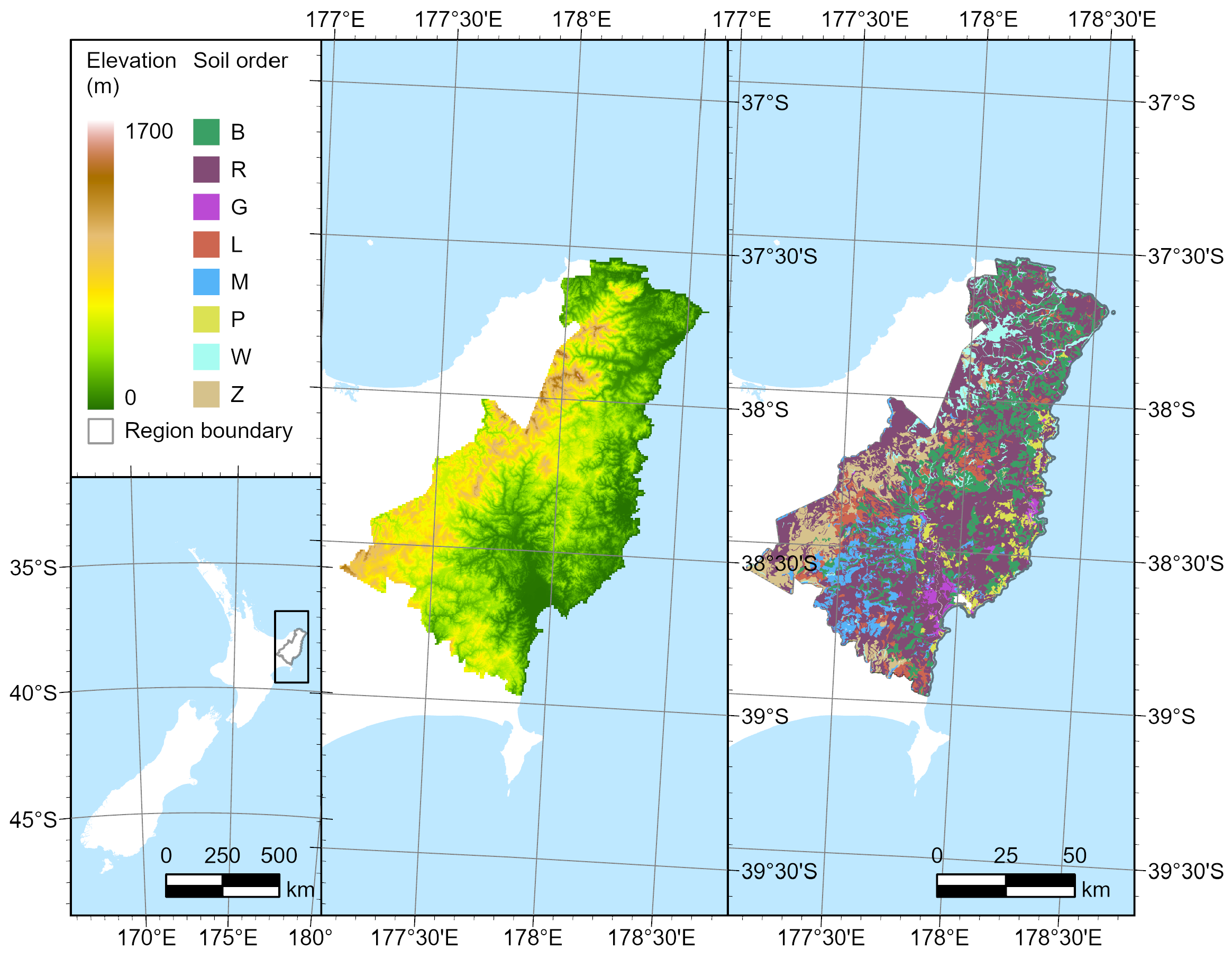
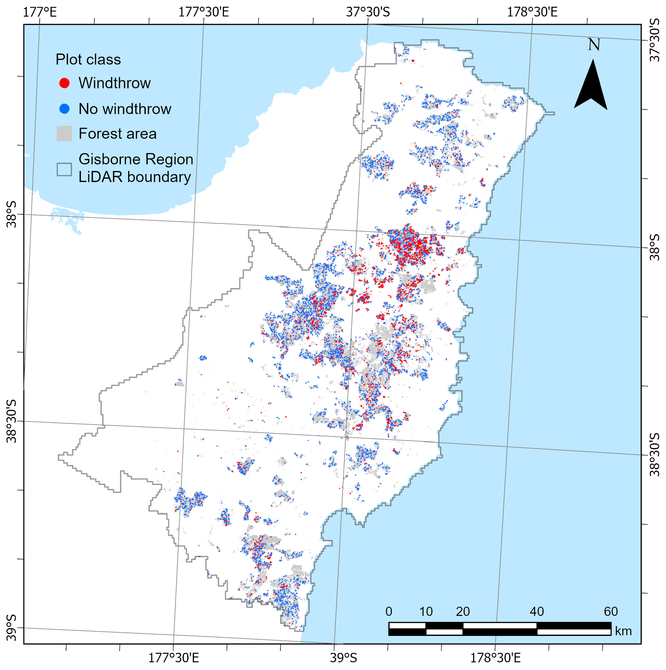
2.1. Study Region

The Gisborne Region was selected for this study because it has a substantial plantation resource that was severely affected by Cyclone Gabrielle, which impacted the North Island of New Zealand from 11 to 15 February 2023. This region covers a wide range in elevation, from the sea level along the eastern and northern coastlines to 1700 metres within western inland regions, with forests covering an elevation range of 1–1222 m (Figure 1). Among the affected North Island regions, rainfall was most intense within the Gisborne Region, which received a total of 531 mm during the event [56]. This is a high proportion of the mean annual rainfall of the region, which ranges from 987 mm in the southeast to 2355 mm/year in the west [57]. Rainfall rates steadily increased over 13 February, reaching a peak of 20–30 mm/h during the night of 13/14 February [56]. The average two-day rainfall accumulation of 230 mm within the Gisborne Region has only been matched once in the past forty years, during the passage of stalled ex-tropical cyclone Bola [55]. This high rainfall was accompanied by strong wind gusts of up to 93 km/h, which, in combination with the rain, caused substantial windthrow, the toppling of trees, and soil erosion. Cyclone Gabrielle was preceded by Cyclone Hale on 10/11 January 2023, with much of the North Island experiencing the wettest January on record [56].

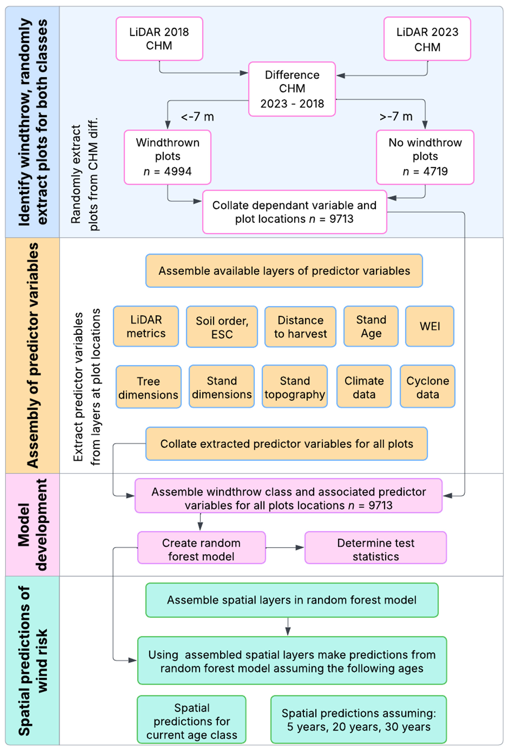
2.2. Overview of Method

The overall modelling workflow followed four main stages, as illustrated in Figure 2. The first stage involved the identification of windthrow areas by differencing pre- and post-cyclone LiDAR-derived canopy height models. Polygons representing areas of canopy loss were manually verified against high-resolution aerial imagery and classified into natural (storm-related), anthropogenic (harvest-related), and landslide features. These verified windthrow polygons were then used to extract plot-level data by randomly allocating points within both windthrown and unaffected forest areas, ensuring the balanced representation of both classes for model training.

In the second stage, a comprehensive set of predictor variables was assembled from remote sensing and ancillary spatial datasets. These included LiDAR-derived stand structure metrics, topography, climate, soils, and stand-level attributes such as age, height, and stand density. In the third stage, a random forest classification model of windthrow was developed using the selected predictors. The final stage involved applying the trained model across the Gisborne Region to generate high-resolution windthrow risk maps under current and simulated stand age scenarios. This structured approach facilitated both robust statistical analysis and operationally useful spatial predictions.

2.3. LiDAR Data

New Zealand initiated a nationally funded program to capture ALS data at a regional scale in 2018. All data are published by Land Information New Zealand (LINZ) and available in a public data repository (https://nz-elevation.s3-ap-southeast-2.amazonaws.com/catalog.json, accessed on 2 February 2025). The initial capture for the Gisborne Region occurred from 31 December 2018 to 9 September 2020, while a subsequent capture was undertaken from 11 September to 16 December 2023 to understand the impact of Cyclone Gabrielle. The specifications for the two captures included a minimum of 4 pulses/m², a vertical accuracy (95%) of ≤20 cm in non-vegetated areas, and a horizontal accuracy (95%) of ≤1 m. The 2018 to 2020 dataset was captured with an Optech Orion H300 LiDAR system (Teledyne Optech, Toronto, ON, Canada), with a scan angle of ±30 degrees, achieving 10.07 pts/m², while the later 2023 capture used a Leica Terrain Mapper (Leica Geosystems AG, St. Gallen, Switzerland), with a scan angle of ±20 degrees, which achieved 30.25 pts/m².

The earlier Gisborne tiles were processed using LAStools version 241106 (rapidlasso GmbH, Gilching, Germany). An automated pre-processing pipeline was applied to the pre-classified point clouds, consisting of the following steps: (i) denoising the raw point clouds using lasnoise; (ii) normalizing the ground of the point clouds with lasheight; and (iii) performing an additional denoising step to remove any remaining extreme points or small isolated clusters. Forest plot point clouds were extracted from the processed data at the end of step (iii) and were later used for individual tree detection and metric extraction.

The module lasnoise employs a noise detection algorithm based on point distribution, identifying points with few neighbours within a specified moving window size, centring the analysis on the respective point’s cell. The two key options were “-isolated”, which controls the number of neighbouring points (set to 5 for this study area), and “-step_size”, which defines the size of the moving window (set to 1 m). This process classified isolated points and small clusters with fewer than 5 points within the 1 m² area as ASPRS class 7 (low or high noise). The module lasheight utilized ground points (ASPRS class 2) to construct a ground Triangulated Irregular Network (TIN), which was then used to normalize point heights by replacing Z-values with ground-normalized heights. For this region, the height range was constrained to 0–80 m. The initial parameters were chosen based on domain knowledge of the forest types and characteristics in the study area, as well as point cloud specifications such as point density and minimum point distance. These parameters were then refined through trial and error by testing different settings in our previous study [58].

Standard LiDAR height metrics were calculated from the normalized point cloud using LAStools at a 10 m resolution. These included the total number of points (all), minimum (min), maximum (max), and mean (avg) heights, along with height distribution metrics such as skewness (skew), kurtosis (kur), and standard deviation (std.dev) within the specified grid. Percentile heights were also computed at the 10th (p10), 25th (p25), 50th (p50), 75th (p75), 90th (p90), 95th (p95), and 99th (p99) percentiles. Additionally, commonly used canopy gap metrics were derived. These included a gap in canopy cover > 2 m (cov.gap), which was calculated as the percentage of first returns above 2 m relative to all first returns. The gap in canopy density > 2 m (dns.gap) was also determined as the percentage of all points above 2 m relative to all returns.

Several LiDAR-derived surfaces describing terrain metrics, including aspect, slope, topographic position index (TPI), and terrain ruggedness index (TRI), were also produced using GDAL at a 10 m resolution. The variables TPI and TRI are measures of neighbourhood variability in elevation. TPI was determined as the difference between a cell value and the average elevation of the eight surrounding cells, with positive and negative values indicating a location is, respectively, higher and lower than its surroundings. TRI was determined as the mean absolute difference between a cell value and its eight surrounding cells, with higher values indicating more rugged terrain. A list of all the LiDAR metrics and variables derived from LiDAR metrics is given in the Appendix A as

Table A1. Variation in LiDAR variables and variables derived from LiDAR metrics for plots with windthrow and no windthrow. The mean and standard deviation (in brackets) and range are shown for plots with no windthrow (n = 4719) and windthrow (n = 4994). Also shown are Kruskal–Wallis ANOVA results, which show the H value followed by the significance category and eta squared (η²). Asterisks *** represent significance at p = 0.001; ns is not significant at p = 0.05. Variables were sorted in descending order of H index for each of the two categories.

Label	Variable	No Windthrow		Windthrow		ANOVA
		Mean (SD)	Range	Mean (SD)	Range	H Val.	η2
LiDAR variables
abv	Number of pixels > 2 m	1145 (669)	3.5–6387	1144 (636)	236–5136	0.080 ns	−9.5 × 10−5
all	Total number of points	1409 (742)	355–7192	1433 (754)	387–6312	1.4 ns	4.2 × 10−5
cov.gap	Gap in canopy cover > 2 m (%)	10.9 (14.4)	0–99.1	11.4 (9.77)	0–86.8	176 ***	0.0181
dns.gap	Gap in canopy density > 2 m (%)	20.7 (14.0)	0.078–99.2	21.2 (9.59)	0.35–82.0	113 ***	0.0115
min	Minimum height value (m)	5.65 (4.78)	0.448–25.2	5.95 (4.74)	2.0–25.4	24.8 ***	0.00245
max	Maximum height value (m)	28.9 (11.0)	0.909–53.8	34.4 (8.24)	9.86–54.3	669 ***	0.0688
avg	Average height value (m)	19.4 (8.43)	0.695–39.9	23.4 (6.7)	5.52–40.4	541 ***	0.0556
p10	10th percentile of height (m)	12.9 (7.14)	0.485–33.3	15.6 (6.7)	2.34–34.5	366 ***	0.0375
p25	25th percentile of height (m)	16.5 (7.92)	0.531–36.6	20.0 (6.75)	3.14–38.6	455 ***	0.0468
p50	50th percentile of height (m)	20.0 (8.8)	0.596–40.4	24.1 (7)	5.45–41.9	541 ***	0.0556
p75	75th percentile of height (m)	22.8 (9.54)	0.680–44.6	27.5 (7.38)	6.91–45.8	604 ***	0.0621
p90	90th percentile of height (m)	24.9 (10.1)	0.815–48.2	30.0 (7.72)	7.97–49.3	643 ***	0.0661
p95	95th percentile of height (m)	26 (10.3)	0.851–49.9	31.3 (7.9)	8.52–50.9	656 ***	0.0675
p99	99th percentile of height (m)	27.7 (10.7)	0.896–52.3	33.2 (8.15)	9.28–52.9	673 ***	0.0692
skew	Skewness of height values	−0.50 (0.54)	−2.56–1.22	−0.68 (0.512)	−2.9–1.31	279 ***	0.0286
kur	Kurtosis of height values	3.67 (1.54)	0.421–14.7	4.07 (1.86)	1.26–19.7	131 ***	0.0134
std.dev	Standard deviation, height (m)	4.76 (2.36)	0.083–15.9	5.72 (2.2)	1.52–16	532 ***	0.0547
LiDAR-derived variables
Aspect	Aspect (degrees)	179 (88.4)	4.7–352	168 (98.2)	2.09–358	39.1 ***	0.00392
Slope	Slope (degrees)	21.8 (7.73)	0.637–49.5	22.6 (8.28)	0.85–50.4	15.6 ***	0.00151
TPI	Topographic position index	0.035 (0.59)	−2.52–2.75	−0.082 (0.678)	−3.97–3.33	64.4 ***	0.00653
TRI	Terrain ruggedness index	11 (4.12)	0.386–30.1	11.2 (4.4)	0.528–30	0.35 ns	−6.6 × 10−5

.

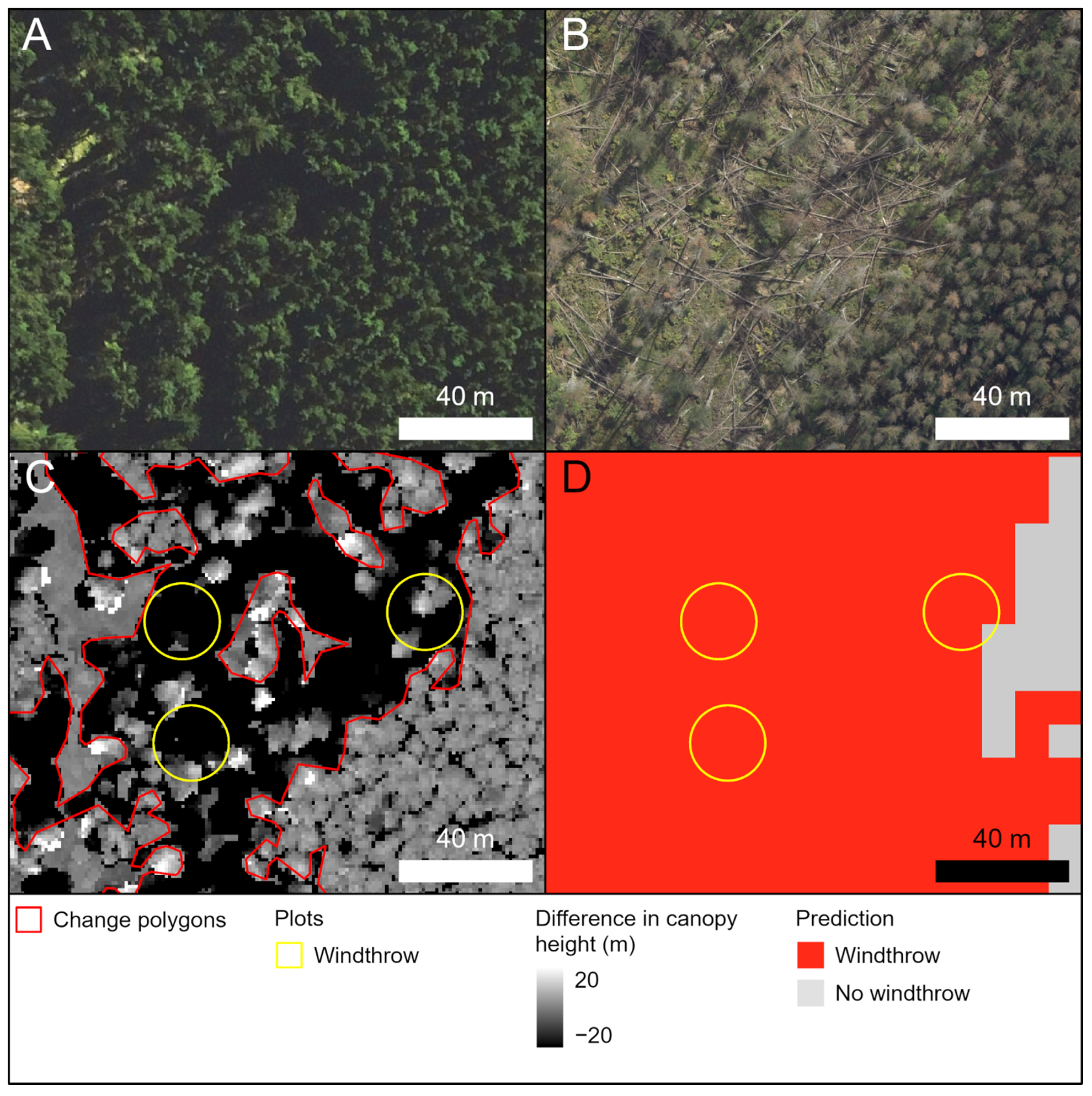
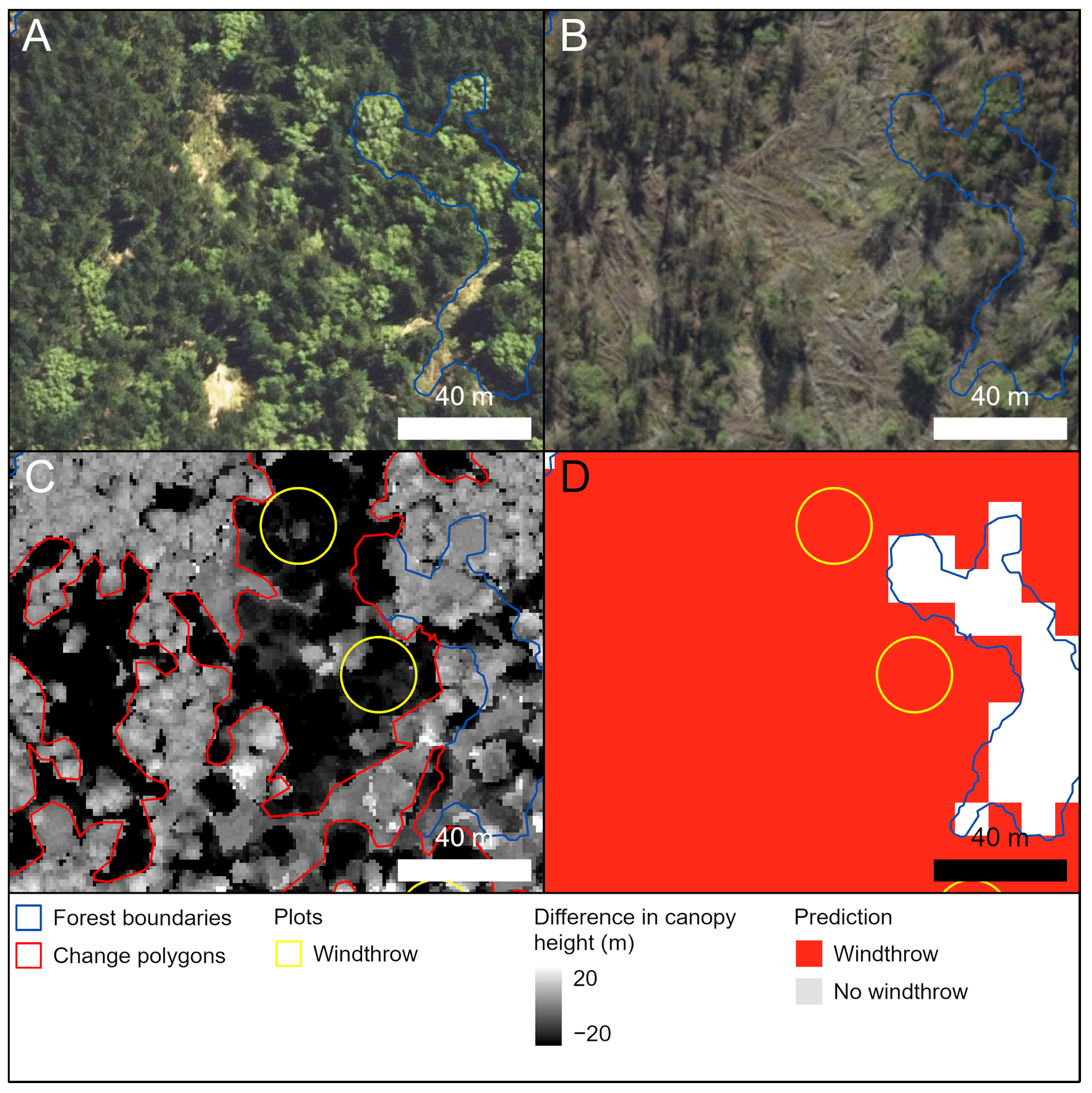
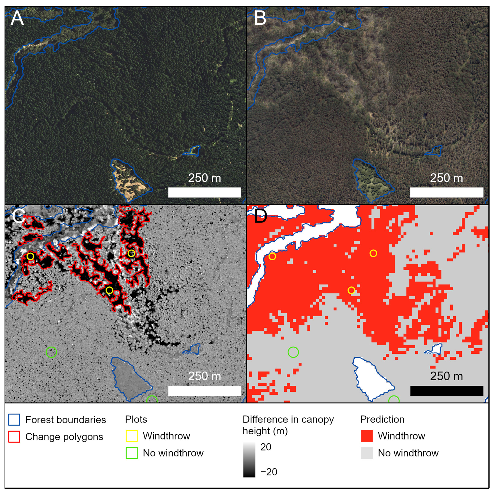
2.4. Plantation Identification and Windthrow Characterization

The base plantation area was identified using an existing forest boundary dataset derived from the earlier regional aerial capture and delineated using a deep learning model [58] (Figure 3A). These forest boundaries were obtained through training a deep learning model using two classes—radiata pine and juvenile plantations—that were pooled together in the final dataset. Although the juvenile plantation class likely comprised other exotic plantation species, the area of these exotic species in the current analysis was negligible, as (i) in total, 97% of plantation species in the Gisborne Region are radiata pine [59] and (ii) the juvenile plantation class represented a small percentage of stands, ranging from 2 to 4 years old [58]. The total identified forest area in the Gisborne Region was 139,336 ha.

Estimates of windthrow were determined using CHMs that were generated prior to and after the cyclone from the LiDAR data at a 1 m resolution. Windthrow was determined by subtracting the CHM of the earlier LiDAR capture from that of the later LiDAR capture using the ArcGIS Pro 3.4.0 raster calculator (ESRI, Redlands, CA, USA). In the resulting difference surface, positive values indicated growth, and negative values indicated a loss in forest height between the two captures, on either side of the cyclone (Figure 3C). By reviewing this difference surface against the post-storm aerial basemap, a loss of 7 m was used to denote windthrow. While the misclassification of windthrow due to using a fixed height loss threshold may occur, this value was considered conservative, as radiata pine stands under 7 m were considered unlikely to suffer from losses related to storms [52]. Additionally, the detected windthrow was reviewed in the later RGB imagery collection for moderate to large areas and appeared to capture windthrow locations well.

The difference surface was filtered in ArcGIS Pro 3.4.0 (majority filter, three rounds, 4 connected) and sieved in QGIS 3.28.6 (40 pixels, 4 connected) to remove noise. It was then converted to a vector, smoothed (PAEK, 8 m), and clipped by the forest boundaries (Figure 3C). Small features were iteratively absorbed into neighbours until a minimum feature size of 0.02 ha was reached. Remaining features were then reviewed by descending size against a subsequent regional aerial capture (2023–2024) (Figure 3B). Features were classed manually into natural (likely storm damage), anthropogenic (harvest activity, road cutting, etc.), and slips (features with no visible stems post-event and attached to existing, i.e., pre-2018–2020 slip features) to a minimum area of 0.6 ha, with the assumption that features below this size were unlikely to be the result of harvesting processes. A total of 3705 ha was identified as windthrown across the forest estate, representing 2.66% of the total forested area of 139,336 ha. Examples of windthrown areas and the resulting classification, showing stems lying on the ground, are shown in the Appendix A as Figure A1, Figure A2 and Figure A3.

The natural change features were then related back to the original forest boundaries, giving a combined dataset split into windthrow and no-windthrow classes. Following inverse buffering to ensure plots would remain entirely within the feature bounds, 5000 points were randomly distributed within both windthrow and no-windthrow classes (i.e., 10,000 plots in total). As the buffered areas were often quite narrow for areas affected by windthrow (Figure 3C), plots that were 400 m² in size were installed, which allowed a relatively large number to be placed across the region. As areas without windthrow were larger and more contiguous, the plot size was increased to 1000 m², which allowed more precise plot-level estimates to be made. An appropriate minimum spacing between points was used to prevent overlapping plots. After a number of plots were removed from the dataset due to the absence of data from predictive spatial layers, the total number of plots available for the modelling was 4994 plots with windthrow and 4719 plots without windthrow (Figure 4).

2.5. Assembly of Predictor Variables

2.5.1. Site Characterization

In addition to LiDAR metrics, data from a range of surfaces that characterized the site were extracted for all plot locations. Site quality was described using the radiata pine site index and the 300 Index. Site index is defined as the mean top height (MTH) at age 20, with MTH defined as the mean height of the 100 largest trees per hectare by diameter. The 300 Index is the mean annual increment in stem volume at age 30 years, for a stand density of 300 stems/ha [60]. Using methods fully described in [60], surfaces for both productivity metrics were developed using a dataset of 3676 nationally distributed permanent sample plots. The two models, which were developed from environmental covariates, had high accuracy on the 30% withheld test dataset for both site index (RMSE of 2.08 m and R² of 0.80) and 300 Index (RMSE of 3.45 m³/ha/yr and R² of 0.68).

Long-term climatic data were extracted from geospatial surfaces that described total rainfall [61], windspeed [61] and drainage [62]. Annual averages for these climatic variables were calculated, along with separate averages specifically for the summer period and individual summer months. Long-term monthly averages were focused on summer to link to the timing of Cyclone Gabrielle, which occurred in late summer.

Erosion susceptibility classification (ESC) is a national dataset that classifies land units into low, moderate, high, and very high risk for erosion and is used in consenting assessments for plantation forestry activities. This dataset was rasterized into a 10 m surface to match the origin and extent of the LiDAR surfaces [63]. Soil orders and potential rooting depth (PRD), derived from the Fundamental Soil Layers [64] were also rasterized. Potential rooting depth describes the depth to a layer that may impede root extension. This threshold layer may be defined by penetration resistance, poor aeration, or very low available water capacity, as described in [65]. Key soil orders within the study area were Brown (B), Gley (G), Allophanic (L), Pumice (M), Pallic (P), Recent (R), Raw (W), and Podzol (Z), with Recent and Brown underlaying 71% of the region area (Figure 1).

The Euclidean distance to harvest was calculated using a 10 m resolution raster distance surface, generated with the QGIS Proximity (raster distance) tool. This surface was derived from harvest features identified during the change detection feature review. The wind exposition index (WEI)—which is a dimensionless metric indicating wind sheltering (values < 1) or exposure (values > 1)—was calculated in SAGA GIS 7.8.2 [66]. A step size of 15 degrees and acceleration of 1.5 were held constant while the search distance was run at 1, 2, 5, and 10 km. Smaller step sizes were tested, but these had very little impact on values of WEI, and for instance, the mean absolute difference between step sizes of 5% and 15% was 0.002207. Comparisons of model performance using the four different search distances for WEI were made in the final two classification models.

2.5.2. Stand Age

Stand age was estimated at the time of the earlier LiDAR capture using a 10 m resolution version of the 2018–2020 CHM, segmented into patches of similar canopy height using the ArcGIS Pro Segment Mean Shift tool. After clipping to forest boundaries, percentile canopy heights (p5, p10, p15, p85, p90, and p95) were calculated per segment. The same height statistics were derived for internal stand data with known establishment years, and a random forest model was trained to predict establishment year for the LiDAR-derived segments based on percentile canopy heights. Using a withheld test dataset comprising 10% of all observations, the establishment year was accurately predicted with an R² value of 0.89 and a root mean square error (RMSE) of 2.88 years. To enhance prediction accuracy, the Hansen Global Forest Change dataset was incorporated where available, as it provides annual forest loss detections from 2001 onward based on loss detections via Landsat time series analysis [67]. The final combined dataset was rasterized to a 10 m resolution, with pixel values representing the estimated year of establishment. Accuracy for the final predictions was assessed by comparing establishment year predictions against the plot data described in Section 2.5.3. This comparison showed 66.7% of intersecting points were within 1 year of the true value, 89.5% within 2 years and 95.8% within 3 years. The stand age at the time of the cyclone (February 2023) was determined from the predicted establishment year for analyses. The method used to develop this spatially explicit age surface is novel and provides a valuable high-resolution input for wind risk modelling.

2.5.3. Stand Dimensions

Forest inventory data from a network of 560 plots, dispersed across the Gisborne Region, were provided by New Zealand Carbon Farming (Auckland, New Zealand) and Ngati Porou Forests Ltd. (Ruatoria, New Zealand) and used to develop models of important stand dimensions. The field data comprised plot locations, plot area, establishment year (used to calculate stand age at the time of analysis), and tree counts. Diameter at breast height (DBH) was recorded for all trees within the plots, and height was measured for a subset of trees in each plot. Measurements were made between 2015 and 2019. The plot data were interpolated into the industry standard software YTGen 3.12.4.0 (Silmetra Ltd., Putaruru, New Zealand) and grown forward in time, at the plot level, to immediately before the cyclone in February 2023, using the 300 Index growth model [68]. Among the generated outputs, variables that were useful for this study included stand density (density), mean diameter at breast height (DBH), and mean top height (MTH).

The dependent variables MTH, DBH, and stand density were predicted using previously described LiDAR and topographic data that were extracted to match the plot locations. All models were developed using R version 4.2.3 [69]. Variable selection was undertaken through randomly splitting the dataset, with 85% used for model fitting and 15% set aside and used for model testing. Multiple regression was used to create the three models from the training dataset using 1st- and 2nd-order polynomial forms for the predictor variables, using a ten-fold cross-validation, with five repeats.

Using an automated selection process, predictor variables were introduced one at a time into each model, starting with the variable that was most strongly related to the stand attribute. Following this initial step, residual values were extracted from the model, and the process was repeated to find the next most strongly correlated variable, with this step repeated until included variables were not significant or improvements in the R² were <0.01. The variance inflation factor (VIF) was used to assess multicollinearity between variables, with values of VIF < 5 indicating an acceptable level [70]. Model accuracy and fit was determined on the test dataset from the root mean square error (RMSE) and R².

Once the key predictor variables were identified, models for the tree dimensions were created using the full dataset. The model for DBH was refined at this stage through using a non-linear regression form to account for changes in DBH with increases in the LiDAR 95th percentile of height (p95) to ensure that DBH approached an asymptote as height increased (DBH = 1/(a + b (p95^−c)). Model statistics for this revised model were determined from the withheld test dataset before fitting the model using the full dataset. The final model formulations were used to estimate MTH, DBH, and stand density for the extracted dataset using the relevant extracted LiDAR and topographic variables. The variables that were included in the models and final model statistics are given in

Table 1. Variation in statistics for multiple regression models describing the three target variables, which include mean top height (MTH), diameter at breast height (DBH), and stand density (SD). Statistics were derived from predictions made on the test dataset and include the coefficient of determination (R²), root mean square error (RMSE), percentage RMSE (RMSE %), and mean bias error (MBE). The units for the RMSE and MBE follow those of the target variable. Also shown are the predictor variables included in each model, which are ranked in order of importance. The full names of these variables are given in Table 2 and Table A1. The variable DSM_SD is the stand density derived from a raster that predicts this variable from a digital surface model (DSM).

Target	Model Statistics				Model Variables
Variable	R2	RMSE	RMSE%	MBE
MTH (m)	0.918	2.65	8.02	0.414	p90
DBH (cm)	0.867	4.21	10.1	−0.506	p95, cov.gap, WEI1km, TRI, skew, TPI
SD (stems/ha)	0.640	179	37.3	−4.09	std.dev, dns.gap, DSMSD, min

. Stem slenderness was defined in units of m/m from these predictions as MTH/(DBH/100).

2.5.4. Tree Dimensions

The LiDAR-derived 1 m CHM was smoothed by applying a 3 × 3-pixel moving window. Individual tree peaks were detected on the smoothed CHM using a local maxima algorithm with a variable window size and a minimum height threshold of 2 m using the lidR package version 4.1.2 [71]. The variable window size was applied to account for varying tree spacing resulting from silvicultural operations, such as thinning, which occur as stands mature. The spacing was initially set to 3 m for points with a height of 2 m and increased by 0.05 times the tree height as the point height exceeded 2 m. This approach was determined through trial and error, starting with a multiplier of 0.01 times the tree height and visually inspecting tree peak detection results across randomly selected sample forest areas of different age classes. These tree peaks were then used as markers for delineating individual tree crowns.

Crown delineation was performed on the smoothed CHM using the “mcws” function within the ForestTools package version 1.0.2 in R [72], which utilizes a watershed algorithm. From the delineated tree crowns, tree height metrics (maximum, mean, and standard deviation) were calculated based on CHM pixels within each crown polygon. Additionally, the 2D crown area (CA) for each polygon was estimated. These metrics were computed for each individual tree polygon on the non-smoothed CHM using the terra package version 1.7-83 in R [73]. A tree stand density raster (DSM_SD) was also created by summing local-maxima-detected tree peaks within a 20 m grid and assigning the total as the pixel value. Predicted values of tree stand density (DSM_SD) and crown area (CA) were extracted for all plots from the layers described above.

2.5.5. Cyclone Characterization

Weather data used in this analysis were sourced from the Virtual Climate Station Network (VCSN), provided by the National Institute of Water and Atmospheric Research (NIWA). The VCSN provides nationwide coverage on a 5 km grid for various weather variables, estimated from data collected by 150 automatic climate stations managed by NIWA and the MetService. For this study, the relevant VCSN variables included daily rainfall, mean relative humidity, and mean windspeed, which have been estimated on a daily basis throughout the Gisborne Region for the duration of the cyclone (11–15 February 2023). As these data were available as points with 5 km spacing, Inverse Distance Weighting was applied in ArcGIS Pro 3.2.1 to create a continuous 10 m spatial surface for each variable for each of the five days of the cyclone (i.e., 15 surfaces). Values for each variable were subsequently extracted from these surfaces for plots with and without windthrow.

2.6. Data Analysis

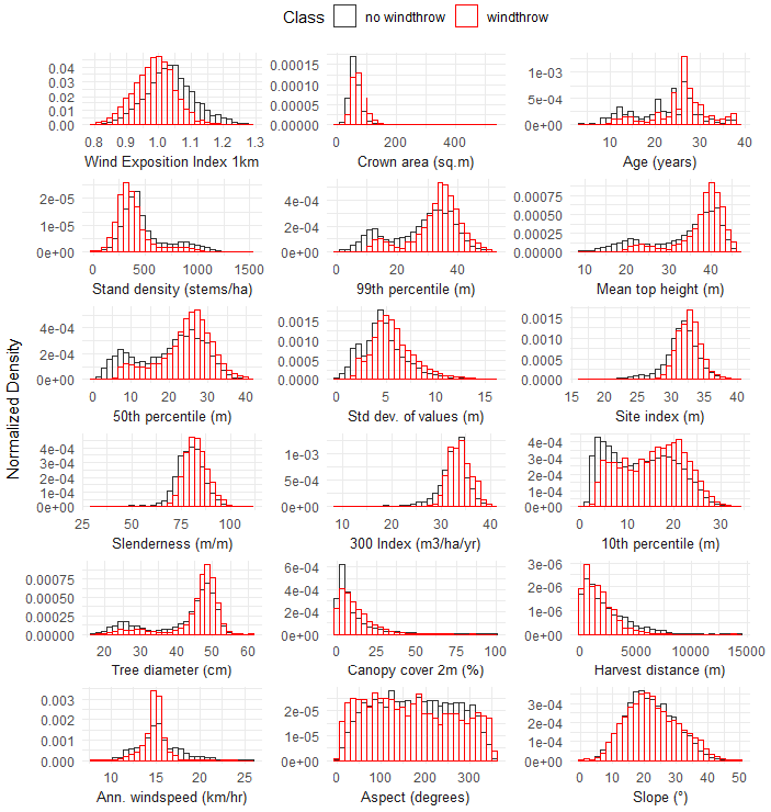
2.6.1. Influence of Individual Variables on Windthrow Classes

Analyses described in this section were undertaken using R version 4.2.3. [69]. Analysis of variance (ANOVA) was used to determine if key site and stand variables differed significantly between the two windthrow classes. As ANOVA relies on the assumptions of normality and homogeneity of variance, diagnostic tests were performed to evaluate the robustness of these assumptions. Specifically, the Shapiro–Wilk test [74] was applied to assess departures from normality, while Levene’s test [75] was used to evaluate the equality of variances across groups. Since all tested variables violated one or both assumptions, the Kruskal–Wallis test [76] was used. The Kruskal–Wallis test is a non-parametric method used to determine whether there are statistically significant differences between the medians of two or more independent groups, making it a robust alternative to ANOVA when the assumptions of normality or homogeneity of variances are violated. The output included the H value, which offers a measure of the overall group differences, and eta squared (η²), which quantifies the effect size, indicating the proportion of variance explained by the windthrow class.

Using chi-square, tests of significance were undertaken to assess whether windthrow class was impacted by the categorical variables soil order and the erosion susceptibility classification. Since a significant overall association does not indicate which specific groups differ from one another, a post hoc test was performed using the Bonferroni adjustment. This multiple range testing method controls for the increased risk of Type I errors when making several pairwise comparisons, ensuring that any detected differences are truly significant.

Histograms were used to visualize the distribution of all important variables. The distributions were plotted by windthrow class (windthrow and no-windthrow) and facetted by variable. For key variables, the relationship between each variable and the proportion of windthrow was explored to identify patterns or thresholds associated with increased windthrow risk. Most continuous variables were divided into 10 equal-sized groups (deciles) to facilitate comparison, while for categorical variables, groupings were created based on their respective classes. For each group, the mean percentage of windthrow plots and the average value of each variable were plotted to identify changes in windthrow with variation in the variable.

2.6.2. Classification Model

Random forest was used to classify the two windthrow classes (windthrow and no-windthrow) using scikit learn, version 0.23.2 [77], which was implemented in Python version 3.9.18. Random forest is an ensemble learning technique that constructs a collection of decision trees during the training process. Each tree is built using a bootstrap sample—a randomly selected subset of the training data with a replacement—and at each node, splits are determined based on a randomly chosen subset of features. This methodology promotes diversity among the trees, which helps mitigate overfitting and improves the model’s ability to generalize to new, unseen data. The final classification is determined by majority voting, where the class label predicted by the most trees is selected as the output. This process enhances both the accuracy and robustness of the model.

Two classification models were constructed. The first model included all site and stand dimensions. A number of relevant long-term climatic variables were also introduced into this first model, including windspeed, rainfall, and site drainage averaged at an annual level and over the summer period. The second model included all variables in the first model and the key characteristics of the cyclone. Given that the first model did not include specific weather information from the cyclone, this model was developed as a generalized method of estimating future potential wind risk in current forests and areas not afforested. The second model was developed to determine how much additional variance cyclone-related variables explained within the current forests.

Recursive feature elimination (RFE) was used for feature selection for both models, utilizing a random forest classifier with a stratified 10-fold cross-validation. The RFE process began with all variables in each dataset and iteratively reduced the feature set down to two variables. At each step, RFE retained the most important variables based on their importance scores while progressively excluding less relevant ones. To mitigate overfitting, pairwise correlations among predictor variables were evaluated, and variables with an absolute correlation coefficient (∣R∣ > 0.9) were flagged. Among highly correlated pairs, the variable with the lower importance score was excluded. Following this process, the variable subset with the highest mean accuracy was output as the optimal starting feature set for subsequent modelling.

After selecting features for the two models, the data were split into a training/test dataset. This division allocated 80% of the observations (3995 windthrown plots and 3775 no-windthrow plots) to a training dataset, while the remaining 20% (999 windthrown plots and 944 no-windthrow plots) were reserved for a test dataset. The random forest model was trained on the training dataset using five-fold cross-validation, and predictions from the trained model were evaluated on the independent test dataset. This procedure was repeated 49 additional times, each with a different train/test split, resulting in a total of 50 iterations. Performance metrics were averaged across all test datasets. This iterative process minimized potential bias from relying on a single train/test split, enabling a more robust assessment of the model’s true performance.

Three hyperparameter grids were evaluated for model fitting that varied in complexity, with the simplest using default parameters and the most complex optimizing model performance across a range of five hyperparameters (i.e., the number of estimators, max depth, min samples split, min samples leaf, and max features). The default hyperparameter grid was selected for the final models, as this had an identical or better accuracy than the models with the more complex hyperparameter grids for both classification models. This grid used 100 estimators, max depth = none, min samples split = 2, min samples leaf = 1, max features = √ (number of predictors), and Gini impurity; all other parameters remained at their default settings.

Using the mean predictions made on all 50 independent test datasets, a confusion matrix was constructed for the two models. The windthrown plots were designated positive, and values in the confusion matrix quantified the percentage of true positives (TPs), true negatives (TNs), false positives (FPs), and false negatives (FNs). Model performance was assessed on the test dataset using precision, recall, F1 score, and accuracy, which were calculated as follows:

$$\mathrm{P}\mathrm{r}\mathrm{e}\mathrm{c}\mathrm{i}\mathrm{s}\mathrm{i}\mathrm{o}\mathrm{n}={\displaystyle \frac{\mathrm{T}\mathrm{P}}{\mathrm{T}\mathrm{P}+\mathrm{F}\mathrm{P}}}$$

(1)

$$\mathrm{R}\mathrm{e}\mathrm{c}\mathrm{a}\mathrm{l}\mathrm{l}={\displaystyle \frac{\mathrm{T}\mathrm{P}}{\mathrm{T}\mathrm{P}+\mathrm{F}\mathrm{N}}}$$

(2)

$$\mathrm{F}1 \mathrm{s}\mathrm{c}\mathrm{o}\mathrm{r}\mathrm{e}=2\times {\displaystyle \frac{\mathrm{P}\mathrm{r}\mathrm{e}\mathrm{c}\mathrm{i}\mathrm{s}\mathrm{i}\mathrm{o}\mathrm{n}\times \mathrm{R}\mathrm{e}\mathrm{c}\mathrm{a}\mathrm{l}\mathrm{l}}{\mathrm{P}\mathrm{r}\mathrm{e}\mathrm{c}\mathrm{i}\mathrm{s}\mathrm{i}\mathrm{o}\mathrm{n}+\mathrm{R}\mathrm{e}\mathrm{c}\mathrm{a}\mathrm{l}\mathrm{l}}}$$

(3)

$$\mathrm{A}\mathrm{c}\mathrm{c}\mathrm{u}\mathrm{r}\mathrm{a}\mathrm{c}\mathrm{y}={\displaystyle \frac{\mathrm{T}\mathrm{P}+\mathrm{T}\mathrm{N}}{\mathrm{T}\mathrm{P}+\mathrm{F}\mathrm{P}+\mathrm{T}\mathrm{N}+\mathrm{F}\mathrm{N}}}$$

(4)

Precision quantifies the fraction of correct positive predictions, whereas recall identifies the fraction of true positives that were accurately detected. High values of precision mean there are few false positives, while high values of recall indicate low numbers of false negatives. The F1 score represents the harmonic mean of precision and recall, serving as a balanced measure of the model’s discriminatory power. F1 scores span a continuum from 0 to 1, with categorizations from 0.5 to 0.7, 0.7 to 0.8, 0.8 to 0.9, and >0.9 signifying poor, acceptable, excellent, and outstanding levels of discrimination, respectively. Accuracy was defined as the percentage of correctly predicted observations of the total observations.

The area under the receiving operating characteristic (AUC-ROC) curve was also used to evaluate model performance. The ROC curve plots the true positive rate (sensitivity) against the true negative rate (specificity) of the model with all possible classification thresholds. The AUC values represent the area under the ROC curve and measure the model’s ability to discriminate between the two classes. AUC values of 0.5 correspond to a situation where the classifier is no better than random (ROC curve along the diagonal), and a value of 1 corresponds to a situation where the model perfectly discriminates between windthrow and no windthrow. As a rule of thumb, AUC values over 0.7 are considered acceptable discrimination between classes, values over 0.8 are excellent, and values > 0.9 represent outstanding classification [78].

2.6.3. Spatial Prediction of Windthrow

Classification model 1 was used to make spatial predictions of windthrow for the entire region. As age was a significant variable within the model, predictions were made under three contrasting ages that included 5, 20, and 30 years. Maps were developed showing variation in wind risk for these three ages. Areas classified as windthrown were identified within the plantation estate, unplanted areas, and the entire region. Summary statistics of these areas were determined for each of the three simulated ages for these three areas and for the actual ages within the plantation estate.

3. Results

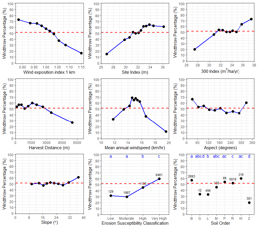
3.1. Variation in Site Characteristics Between Windthrow Classes

All site characteristics significantly varied between the two windthrow classes (

Table 2. Variation in key site, stand, and LiDAR variables for plots with windthrow and no windthrow. The mean and standard deviation (in brackets) and range are shown for plots with no windthrow (n = 4719) and windthrow (n = 4994). Also shown are Kruskal–Wallis ANOVA results, which show the H value followed by the significance category and eta squared (η²). Asterisks, *** and **, represent significance at p = 0.001 and 0.01, respectively. Variables were sorted in order of descending H index for each of the three categories.

Label	Variable	No Windthrow		Windthrow		ANOVA
		Mean (SD)	Range	Mean (SD)	Range	H Value	η2
Site variables
WEI1km	Wind exposition index 1 km	1.04 (0.077)	0.807–1.29	0.99 (0.064)	0.797–1.28	1081 ***	0.1110
SI	Site index (m)	31.5 (2.75)	16.3–39.5	32.7 (1.87)	17.6–40.1	520 ***	0.0535
300 Index	300 Index (m3/ha/yr)	32.4 (3.17)	8.84–40.8	33.8 (2.34)	12.2–40.9	408 ***	0.0419
HD	Harvest distance (m)	2124 (1919)	18.0–14330	1561 (1295)	13.2–13,991	135 ***	0.0138
WindAnn	Mean annual wind (km/h)	15.4 (2.57)	7.80–25.6	14.8 (1.37)	7.79–24.0	67.3 ***	0.0068
Aspect	Aspect (degrees)	179 (88.4)	4.7–352	168 (98.2)	2.09–358	39.1 ***	0.0039
Slope	Slope (degrees)	21.8 (7.73)	0.637–49.5	22.6 (8.28)	0.85–50.4	15.6 ***	0.0015
PRD	Potential rooting depth (m)	1.22 (0.157)	0.23–1.35	1.22 (0.171)	0.35–1.35	8.69 **	0.0008
Stand dimensions
CA	Crown area (m2)	61.4 (19)	2.5–191	74.8 (25.1)	29.3–536	880 ***	0.0905
Age	Age (years)	22.1 (7.01)	13,971	25.8 (6.11)	14,336	780 ***	0.0802
SD	Stand density (stems/ha)	490 (234)	20–1456	384 (189)	20–1534	760 ***	0.0782
MTH	Mean top height (m)	33.7 (8.56)	8.54–45.9	37.9 (5.73)	18–46.1	643 ***	0.0661
Slend.	Stem slenderness (m/m)	79.1 (8.19)	30–108	82.7 (5.98)	63.2–110	517 ***	0.0532
DBH	Tree diameter (cm)	42.4 (9.5)	17–56.2	45.9 (6.86)	17.9–61	315 ***	0.0324
Key LiDAR metrics
p99	99th percentile of height (m)	27.7 (10.7)	0.896–52.3	33.2 (8.15)	9.28–52.9	673 ***	0.0692
p50	50th percentile of height (m)	20 (8.8)	0.596–40.4	24.1 (7)	5.45–41.9	541 ***	0.0556
std.dev	Standard deviation of height (m)	4.76 (2.36)	0.083–15.9	5.72 (2.2)	1.52–16	532 ***	0.0547
p10	10th percentile of height (m)	12.9 (7.14)	0.485–33.3	15.6 (6.7)	2.34–34.5	366 ***	0.0375
cov.gap	Gap in canopy cover > 2 m (%)	10.9 (14.4)	0–99.1	11.4 (9.77)	0–86.8	176 ***	0.0181

). As evidenced by the η² value, differences were most marked for wind exposition index to 1 km (WEI_1km). There was a marked left shift in the distribution for windthrown sites, indicating these areas more frequently occurred within sheltered sites (Figure A4). As WEI_1km increased from 0.88 to 1.15, the percentage of windthrown plots declined from 73% to 16% (Figure 5). The two indices (i.e., site index and 300 Index) were the next strongest site variables. Windthrown plots more frequently occurred at higher values for both indices, with the percentages increasing from 20 to 72% across the 300 Index range and 15% to 61% across the site index range (Figure 5).

Harvest distance also strongly and significantly varied between windthrow classes. Mean harvest distances were 1561 and 2124 m, respectively, for plots with and without windthrow (Table 2). The percentage of windthrown plots mostly ranged from 53 to 60% across harvest distances ranging from 99 to 2638 m, above which this percentage dropped markedly to 27% as harvest distances further increased to 5511 m (Figure 5). Windthrow was significantly affected by mean annual windspeed, and the percentage of windthrown plots increased from 33% at low windspeed to broad maxima of 62–68% between windspeeds of 14.6–15.7 km/h before declining at windspeeds above this point (Figure 5). Windthrow was relatively invariant to slope across most of the range but increased markedly at very high slopes. The windthrow percentage reached a peak on north/northwest-facing aspects (Figure 5).

The two soil-related variables also significantly (p < 0.001) influenced windthrow percentage. There was a consistent increase in windthrow percentage as erosion susceptibility classification (ESC) increased (Figure 5). There was no significant difference in windthrow between lower–moderate-ESC groups, which had windthrow percentages ranging from 30 to 32%. However, windthrow percentage increased sharply to 45% for high-ESC sites and 60% for very high-ESC sites, with this latter class constituting the majority of the four classes (n = 6461 plots). Windthrow in both high- and very high-ESC sites was significantly higher than in lower–moderate-ESC sites, and very high-ESC sites were significantly higher than all other classes (Figure 5)

Among the eight soil orders present within the sampled plots, there were six that had more than 100 plots within the order (Figure 5). The largest departures from the expected class split of 51.4% (dashed red line, Figure 6) for these six soil orders were noted for the Podzols (19.3% windthrow), Allophanic (32.7% windthrow), and Pumice (45.3% windthrow) soil orders, which all had lower-than-expected windthrow. Multiple comparison testing showed windthrow percentage on Podzols to be significantly lower than that for the other soil orders (Figure 5). Conversely, more subtle increases above the expected windthrow percentage (51.4%) were noted for the Brown (56.9%) and Raw (59.7% windthrow) soil orders (Figure 5).

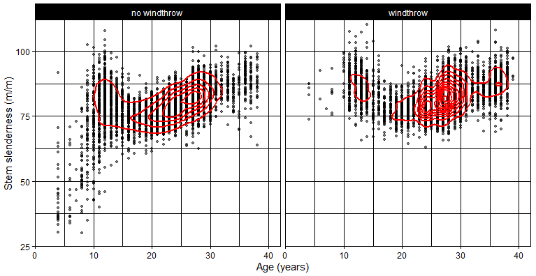
3.2. Variation in Stand Characteristics Between Windthrow Classes

All stand dimensions had a significant impact on windthrow (Table 2). Compared to the site characteristics, stand variables and LiDAR-derived proxies for stand characteristics were generally quite important, constituting 7 of the 10 variables that differed most between the two plot classes (Table 2, Figure A4). According to the η² value, crown area was the most important stand attribute (Table 2). Windthrown plots had a crown area that was on average 22% higher than plots without windthrow (74.8 vs. 61.4 m²) (Table 2). The windthrow percentage increased almost linearly across the range in crown area from 25% to 78% (Figure 6). The percentage of windthrow increased markedly with age from <20% at ages up to 10 years to >74% for stands with ages ≥ 38 years (Figure 6). There were marked reductions in windthrow percentage with stand density, which may largely reflect the increases in windthrow with stand age, as stand density declines markedly with stand age.

Of the standard tree dimensions, MTH was the strongest determinant of windthrow, followed by stem slenderness and then tree diameter (Table 2). Generally, windthrow percentage increased across the range of all three variables (Figure 6). Windthrow percentage reached a threshold of 60–65% at MTH > 40 m and similarly reached a peak of 57–59% at DBH values > 46 cm (Figure 6). However, windthrow percentage increased continuously from 20 to 65% across the entire 68–93 m/m range in stem slenderness (Figure 4). A plot of age against stem slenderness shows very little windthrow below ages of 10 years and stem slenderness values of 63 m/m (Figure 7). Similarly, the maximum data density for windthrown plots is located at higher values of age and stem slenderness than plots without windthrow (Figure 7, red contour lines).

3.3. Classification Models

Classification model 1, which included site- and stand-level characteristics, had excellent performance. Using mean values from 50 iterations on the test dataset, the accuracy and F1 score were, respectively, 0.835 and 0.841 (

Table 3. Confusion matrix and classification statistics for models 1 and 2. Abbreviations for the confusion matrix are as follows: true negative (TN), false positive (FP), false negative (FN), and true positive (TP). The classification statistics included accuracy, precision, recall, F1 score, and the area under the receiving operating characteristic curve (AUC).

Model	Confusion Matrix (%)				Classification Statistics
	TN	FP	FN	TP	Accuracy	Precision	Recall	F1 Score	AUC
1	39.8	8.8	7.7	43.7	0.835	0.832	0.851	0.841	0.913
2	40.1	8.5	7.3	44.1	0.841	0.838	0.857	0.847	0.917

). The precision and recall were 0.832 and 0.851, respectively, indicating that false positives were slightly more common than false negatives. Furthermore, the model achieved an AUC-ROC of 0.913, underscoring its exceptional ability to discriminate between classes (Table 3). A total of 10 continuous variables were included in the model (Appendix A,

Table A2. Variable importance scores for models 1 and 2. Model 1 included site- and stand-level variables, mean windspeed in February (Wind_Feb), and drainage during summer (Drain_Sum). Variables are sorted in descending order of variable importance, according to model 1.

Variables	Model 1	Model 2
WindFeb	0.154	0.103
WEI1km	0.143	0.135
DrainSum	0.106	0.078
Age	0.098	0.084
300 Index	0.097	0.076
Site index	0.090	0.068
Harvest distance	0.087	0.070
Aspect	0.079	0.070
Slope	0.072	0.065
Erosion susceptibility classification	0.034	0.028
Potential rooting depth	0.020	0.015
Recent soil order	0.0082	0.0060
Brown soil order	0.0078	0.0052
Allophanic soil order	0.0031	0.0025
14 February relative humidity		0.078
14 February windspeed		0.060
13 February rainfall		0.056

). The erosion susceptibility class was also included, as were categories for three of the soil orders.

Mean windspeed in February was the most important variable, followed by the wind exposition index and then mean drainage during summer (Table A2). Age was the fourth most important variable and the only stand variable in the model. The productivity surfaces, 300 Index, and site index were the next most important, followed by harvest distance, aspect and slope, erosion susceptibility classification, and potential rooting depth. The Recent, Brown, and Allophanic soil orders were of the least importance in the model (Table A2).

Classification model 2, which included data from spatial layers describing the cyclone, provided very little additional explanatory power over the first classification model. There were increases of less than 0.01 between these two models in accuracy (0.841 vs. 0.835), F1 score (0.847 vs. 0.841), and AUC-ROC scores (0.917 vs. 0.913) (Table 3). Model 2 included all variables in model 1 and three variables of moderate importance, describing total rainfall on 13 February 2023 (importance: 0.056), mean relative humidity (importance: 0.078), and mean windspeed (importance: 0.060) on 14 February 2023. With a few minor changes, the variable importance scores for all other variables in model 2 were very similar to those of model 1 (Table A2). For both classification models, the use of a 1 km search radius for wind exposition index (i.e., WEI_1km) generally yielded comparable or superior performance to other search distances. For instance, values of AUC-ROC for model 2 were, respectively, 0.917, 0.917, 0.916, and 0.916 for search distances of 1, 2, 5, and 10 km.

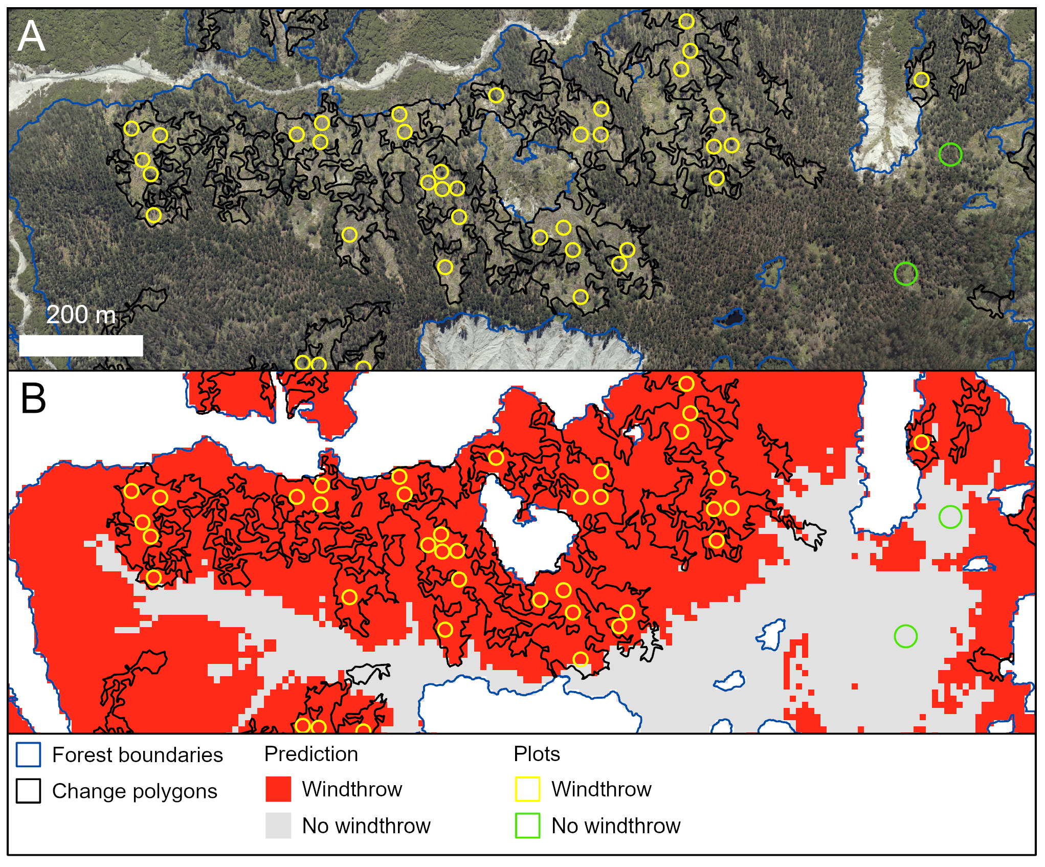
3.4. Predictions of Windthrow

As shown by the representative forest area in Figure 8, predictions from model 1 aligned closely with the plot data. The agreement between plot data and predictions was very high for both windthrow classes (Figure 8). Predictions for the windthrow class did extend beyond the areas that were windthrown in many areas, as can be seen by a comparison of the unaffected areas (Figure 8A) with model predictions (Figure 8B). This aligns with the higher number of false positives than false negatives found within the model, suggesting that model predictions are likely representative of areas that are subject to moderate to high wind risk.

Predictions of windthrow are shown as a percentage in

Table 4. Percentage of predicted windthrow within the plantation estate using the current age structure. Also shown are predictions within the current estate, unplanted area, and entire region, by simulated age classes of 5, 20, and 30 years. Shown for reference is the percentage area in the very high category of the erosion susceptibility classification (ESC) for each area.

Category	Current Estate	Unplanted Area	Entire Region
Age within current estate	23.9%
Simulated age
Age 5	1.5%	0.4%	0.6%
Age 20	20.2%	9.5%	11.2%
Age 30	34.3%	20.9%	23.1%
ESC very high category	55.4%	35.1%	38.3%

and spatially in Figure 9 for the current regional radiata pine estate (Figure 9A) and for the entire region, assuming plantation ages of 5 (Figure 9B), 20 (Figure 9C), and 30 (Figure 9D) years. Predictions of windthrow within the current plantation estate comprised 23.9% of the area. Predictions of windthrow for a given age showed a marked increase from 1.5% of the plantation estate at age 5 to 20.2% and 34.3%, respectively, at ages 20 and 30 years (Table 4, Figure 9).

In contrast, predictions of windthrow within the unplanted area were markedly lower for a given age than those within the plantation estate, increasing from 0.4% at age 5 to 9.5% and 20.9%, respectively, at ages 20 and 30 years (Table 4; Figure 9). Predicted values of windthrow for the entire region were intermediate between those for the current estate and unplanted area at the three ages examined (Table 4). However, it is worth noting that not all of these unplanted areas will be suitable for afforestation.

As a point of reference, predictions of windthrow were compared to the percentage of area covered by the very high-ESC category, which has been used to identify areas at risk of erosion within the region (Table 4). Model predictions of windthrow risk within the current estate were markedly lower than the percentage area covered by the very high-ESC category (23.9% vs. 55.4%). This was also the case for predictions simulated at age 30 for the current estate (34.3% vs. 55.4%), unplanted area (20.9% vs. 35.1%), or the entire region (23.1% vs. 38.3%).

4. Discussion

4.1. Use of Repeat LiDAR Captures to Identify Windthrow

This study demonstrates the effectiveness of repeat LiDAR coverage for identifying and characterizing windthrow at regional scales. Advances in LiDAR technology, including higher pulse densities and improved horizontal and vertical accuracy, have enabled the capture of more reliable, high-resolution data across large areas. By integrating pre- and post-windthrow LiDAR captures, this study provides a detailed assessment that accounts for baseline conditions, offering a significant advantage over single-capture approaches. Windthrow predictions were rigorously validated using post-cyclone aerial imagery, yielding an objective assessment of cyclone damage. The analysis conservatively estimated there to be at least 3705 hectares of windthrow, representing 2.66% of the total forested area. This spatial information is critical for insurance claims, policy decisions, and the strategic allocation of resources, particularly for the timely salvage of windthrown timber before sapstain reduces its value [79]. Importantly, this dataset establishes the first spatial baseline in New Zealand against which damage from future cyclones can be compared. The methodological framework presented here, leveraging multi-temporal LiDAR data, is applicable beyond New Zealand, providing a robust, scalable approach for assessing storm damage in forestry sectors internationally.

Remotely sensed data, extracted across broad spatial scales, was found to be a very valuable data source for the wind risk model developed in this study. Compared to traditional plot-based measurements, the use of remote sensing considerably reduces time, cost, and labour whilst improving the spatial description of affected areas. The method used here was particularly effective, as the pre-cyclone plantation boundaries were accurately delineated using deep learning [58], which reduced the volume of LiDAR that needed to be analyzed to detect windthrow.

Remotely sensed windthrow detection is both scalable and repeatable, making it well suited for comparing disturbance events over time. Regular LiDAR acquisitions are relatively unlikely at a regional scale within New Zealand due to cost constraints. However, the impacts of further cyclones could be determined by the height differencing approach through the acquisition of imagery, from either satellite or fixed-wing aircraft. These data can be used to determine tree height directly from the imagery [80] or through using photogrammetric point clouds [81]. The application of this method across regions and events could be readily used to assemble post-event data from a range of cyclones for the development of a meta-model of wind risk, which could establish a generalized framework for risk assessment. The regional retrieval of disturbance information has application beyond cyclone damage and has, for instance, been recently used to identify disease risk in the Gisborne Region [14].

Although this study successfully identifies the presence or absence of windthrow, distinguishing between different intensities or severities remains technically challenging. Current mechanistic wind risk models, such as ForestGALES using the Turning Moment Coefficient (TMC) method, have been used to quantify damage intensity [38] and damage to infrastructure [82]. Integrated frameworks like iLand, which incorporate ForestGALES, have also demonstrated this capability [83]. Despite this technical feasibility, widespread application is constrained primarily by difficulties in acquiring the necessary detailed input data. These input data include individual tree attributes, precise wind climate measurements [38,83], and, importantly, wind storm data, including wind speed and direction [82]. Future research could address these limitations by combining mechanistic modelling with multi-scale remote sensing methods, including LiDAR and high-resolution optical or multispectral imagery and detailed wind storm data, to improve the accuracy with which windthrow intensity can be detected.

4.2. Wind Risk Model

The wind risk model developed in this study demonstrated excellent performance, underscoring its reliability for practical applications. It is difficult to directly compare the accuracy of our model with previous empirical models due to variations in reported statistics, the types of forests and spatial scale, and the resolution of predictions. However, the accuracy of our modelling approach (0.84) was relatively high compared to previous approaches, which report accuracies ranging from 0.73 to 0.81 [44,51]. Similarly, the AUC scores for both random forest models (0.913–0.917) generally exceeded those of previous studies that mostly range from 0.51 to 0.90 [44,46,52,84] but were less than in one study where the AUC reached values of 0.99 [45]. Our results aligned with other studies comparing modelling methods that show random forest provides robust and accurate predictions of storm damage [44,45,46]. An innovative element within this study was the use of 50 random train/test splits, which provided an unbiased evaluation of model performance and an uncommon level of rigour for empirical wind risk modelling.

The approach used here has a number of advantages. Even if the specific model that was developed is not generalizable, the procedures for data source identification, data gathering and processing, and interpretation are of great value and are themselves applicable to other situations. Through the compilation of these datasets, the second strength of this approach is that it allows the identification and estimation of the importance of key variables. Further research should use the framework developed here during future storm events to compare the relative contribution of different predictors and therefore assess the generalizability of the model. At the very least, it is likely that the accumulation of data from many storm events will provide the opportunity to develop a more generally applicable meta-model. The strong model performance in this study highlights the value of combining machine learning with spatially explicit remotely sensed data to support regional-scale wind risk assessments worldwide. The identified influential variables—such as wind exposure, stand age, and site productivity—are commonly available across global plantation forestry systems. This widespread availability suggests that similar predictor frameworks could be effectively employed in other regions susceptible to cyclones or severe wind events.

4.3. Important Factors Influencing Wind Risk

The variables highlighted by the model have been found to be useful predictors of wind risk. Of greatest importance were the long-term mean February windspeed and the site topographic exposure, as characterized by the WEI. The increasing levels of damage up to medium windspeeds were expected. The reductions in damage that occurred from medium to high windspeeds may reflect adaptation by trees to high windspeeds, which has been shown to reduce stem slenderness [85,86,87,88] and stabilize root systems [89]. This observation was consistent with the response of windthrow to topographic exposure as characterized by WEI_1km. There was a significant negative relationship between WEI_1km and stem slenderness (p < 0.001; R² = 0.18), which agreed with previous research [90], indicating that trees in sheltered areas had significantly higher slenderness and were therefore less adapted to high windspeeds than those located in areas with high WEI, such as ridges.

The windthrow patterns from Cyclone Gabrielle align with established stand-level wind risk factors, e.g., [47]. Among the stand-level metrics, canopy area emerged as the best predictor of damage, most probably as it integrates the key factors of tree height, diameter, and stand density. This finding highlights the utility of individual tree canopy metrics derived from LiDAR for regional wind risk assessments. Stand age, the second most important factor, is a convenient risk metric, often available from forest inventories. Stands younger than 10 years rarely experienced windthrow (Figure 6), reinforcing the link between stand age and height, a well-known wind risk factor [91]. Tree height influences wind damage both directly and indirectly through related metrics like stem slenderness, which was a strong risk indicator—trees with lower height–DBH ratios were at reduced risk, which is consistent with the literature [92,93,94].

Stand density also played a significant role, with denser stands exhibiting lower windthrow risk. This relationship is complex, depending on stand age, silvicultural history, and prior disturbances. Denser stands have been found to reduce wind penetration and lower wind loading and subsequent risk [95]. Previous studies have found that heavy or late thinning increases the short-term susceptibility of a stand to wind damage [96,97]. The initial increase in tree vulnerability after thinning declines with time as the crown recovers [98] and the stem and roots respond to the new wind environments and changes in soil moisture [99].

Aspect, slope, and erosion risk were also significant but less important predictors of wind damage. Most damage was noted for trees on NNW aspects, which is the direction of the prevailing wind in the Gisborne Region. Trees facing this aspect had likely acclimated to that wind direction through developing root systems in windward and leeward directions to maximize anchorage to withstand NNW winds, which is a previously noted response [89]. Consequently, the predominant ESE direction of the storm would have caused significant strain to these trees, resulting in higher rates of windthrow. The risk was further increased on steep slopes and sites with high soil erosion, where limited rooting depth most likely compromised tree stability.

Soil characteristics had a significant influence on wind damage. Windthrow severity varied by soil type, with the most damage observed on Raw, Brown, Pallic, Recent, and Pumice soils, decreasing in that order. In this study, we were unable to differentiate between the two modes of whole-tree damage (stem breakage or tree uprooting), which might introduce some uncertainty in the interpretation of the impact of soil type when discriminating between damaged and undamaged areas. This is because when tree anchorage is poor (e.g., in waterlogged soils or soils with low shear strength), uprooting is typically observed as the type of damage [100]. Conversely, stem breakage is observed more frequently where soils of high shear strength provide better tree stability [101].

Raw soils, often shallow and found on slopes with high water tables, with advanced erosion and rocks at shallow depths, often limit stable root development. When characterized by high water tables, e.g., near rivers, they easily become fluid and consequently have very low soil shear strength, affecting tree stability. One of the early phases of windthrow is related to the slippage of the root–soil plate when soil shear strength is low [100]. Pallic soils pose similar constraints with regard to rooting depth, as they are prone to erosion and waterlogging. Brown and Recent soils, which are both highly fertile, support vigorous growth, increasing windthrow risk. Tree anchorage in brown earth soils is typically solid, due to the high shear strength [102]. In a static tree-pulling study of radiata pine grown on various soil types, Moore [54] reported that trees established on yellow-brown earths exhibited superior anchorage compared to those on other soils. The experiments in Moore [54] were performed in dry conditions, when the shear strength of brown earth soils is not reduced. During Cyclone Gabrielle and the weeks preceding the event, extremely high precipitation was recorded in the Gisborne Region, likely reducing the shear strength of cohesive soils such as brown earths. Similarly, Pumice soils, characterized by low strength, may weaken further under heavy rainfall.

Windthrow was less prevalent on Gley, Allophanic, and Podzol soils (Figure 5). These soils typically do not support vigorous growth, reducing vulnerability to wind damage. Allophanic soils, in particular, allow deep rooting and experience lower erosion, enhancing stability. Surprisingly, Gley soils, which often have high water tables and restrict rooting depth, and whose shear strength is reduced under waterlogged conditions, exhibited less damage—but the low damage on these soils was most likely due to an insufficient sample size (n = 12 plots) to characterize the response.

Edge effects are known to influence wind damage dynamics in forest stands. This occurs both through changes in wind speed profiles at transitions between land use types with differing surface roughness [103] and through the acclimation of edge trees to the harsher wind conditions typically found along upwind stand boundaries [104]. When a stand edge is exposed following the removal of an adjacent stand (e.g., from harvesting or a natural disturbance), wind damage risk to the retained stand increases significantly while the newly exposed edge trees acclimate to their new wind climate [91]. We did not include the impact of edge effects in our wind damage models because of the considerable additional complexity of mapping recent harvests across the landscape. This omission might have impacted the predictive power of our random forest modelling, and future modelling efforts should seek to incorporate edge and acclimation effects [103].

4.4. Planning and Management Implications

From a forest planning perspective, the model and risk maps developed here enhance climate resilience by providing a tool to mitigate the impacts of severe storm events, which are likely to become more frequent [20]. By identifying areas most prone to windthrow, the research informs future planting decisions and plantation layout guidelines. In high-risk zones, alternative windfirm species such as redwood [105] or more robust silvicultural regimes such as continuous cover forestry [106] could be considered as a way to reduce the risk of future forest area losses. The approach used here refines the current erosion susceptibility classification (ESC) red zone class, designated as high risk for future afforestation. This red zone class is improved by incorporating more than just topographic and soil data, reducing the overall risk area while maintaining spatial agreement with existing layers. Predictions of wind risk shown here could support the development of a more targeted planting risk surface beyond ESC and are complementary to the Landslide Susceptibility and Connectivity surface recently commissioned to guide future planting locations.

Management interventions are crucial to mitigating risks, as findings indicate that rotation lengths exceeding 30 years significantly increase vulnerability. This has implications for long-rotation forests and stranded assets, such as those identified within the Gisborne Region in [58], which are likely to be at high risk of windthrow. The creation of detailed risk maps can help identify areas requiring targeted management strategies. For example, coordinating harvest schedules across multiple forest growers and strategically opening harvest areas adjacent to older stands can help reduce exposure. Additionally, implementing early thinning reduces overall risk as younger stands are less vulnerable and have time to readjust to the environment before reaching a more vulnerable stand age. As younger stands have lower value, this strategy also avoids exposure of older, higher-value stands to significant risk. In high-risk areas, reducing rotation lengths and incorporating riparian plantings could further strengthen resilience against windthrow. The management strategies and interventions discussed here, such as rotation shortening and targeted thinning, are universally applicable strategies for forest managers aiming to mitigate windthrow risks in plantation forests. These approaches are particularly valuable in areas across the globe undergoing rapid plantation expansion or facing increasing climatic uncertainties.

Our approach could be made more repeatable, scalable, and useful to managers through the development of methods to continuously monitor changes in forest dynamics and windthrow. NASA’s Global Ecosystem Dynamics Investigation (GEDI) is a LiDAR sensor, attached to the International Space Station, based on the principles of LiDAR that acquires discontinuous data along tracks with a footprint size of 25 m [107]. Through fusing GEDI data with information from other earth observation satellites (e.g., Landsat 8 OLI), global wall-to-wall maps of canopy height at fine spatial resolution have been produced, and similar maps for aboveground biomass density (AGBD) are underway that will provide a global benchmark with well-characterized uncertainty [108,109]. GEDI data are freely available, and if estimates of height could be calibrated using regional LiDAR, then predictions from GEDI could form part of a regular monitoring programme.

While GEDI provides valuable canopy height and structure data at ~25 m resolution, it may not capture small-scale windthrow events. However, it remains a useful tool for detecting larger windthrow-affected areas that may warrant further investigation using higher-resolution data sources or targeted field assessments. Integrating satellite LiDAR with targeted airborne or UAV-based LiDAR could help bridge scale gaps and significantly enhance long-term assessments of biomass change, windthrow impact, and forest recovery. However, the relatively low sampling densities of current spaceborne LiDAR systems—and the resulting need for hybrid approaches—are likely to persist even with recently launched or upcoming platforms such as China’s Gao Fen-7 and Japan’s MOLI [108,110]. Looking ahead, future LiDAR missions may offer improved resolution and revisit frequency, enabling finer-scale change detection and more comprehensive monitoring.

Digital aerial photogrammetry (DAP), from overlapping images, has also been highlighted as a promising technique for large-scale forest inventory [111,112]. When combined with ALS-derived digital terrain models, DAP point clouds have been shown to produce comparable results to ALS at substantially reduced costs, even when scaled to large areas [113,114]. DAP has the added advantage that it can be generated from appropriately designed aerial imagery campaigns [114], potentially providing both high-resolution imagery and 3D data. Photogrammetric point clouds from satellites such as Pléiades have also been used to predict both height and volume in radiata pine with an accuracy similar to that of ALS [81], which showcases the potential value of this method for large-scale regular monitoring. Alternatively, a monocular depth estimation foundation model trained on imagery—called depth anything—has been developed recently, allowing predictions of height from single RGB images [115]. Using this method, a deep learning model could be developed to infer canopy height from either aerial or satellite imagery using regional LiDAR as a ground truth reference. This method could provide a scalable and inexpensive solution for regular regional canopy height estimation.

The development and implementation of these methods for characterizing changes in tree height and biomass would facilitate the continuous monitoring of forest dynamics and wind damage over time. With consistent monitoring using calibrated satellite remote sensing, insights could be obtained quickly for early damage assessments, allowing for mitigation of further damage in areas at risk and faster responses to windthrown areas. This type of real-time information is critical after events such as Cyclone Gabrielle, where road blockages and health and safety issues delayed access to many stands.

4.5. Study Limitations and Further Research

There were a number of limitations within this study. The complex nature of wind damage can make it difficult to automate the identification of windthrow within discrete polygons. Consequently, our predictions of actual wind damage, which amounted to 2.66% of the plantation estate, may be an underestimate as they most likely omitted very small areas of damage. In contrast, the predictions of wind damage from the random forest model, which constituted 23.9% of the estate, were an overestimate, and the model predictions of windthrow often extended beyond the observed damage (Figure 8B). While many of these false positives did not correspond to actual windthrow, they may still reflect areas of moderate to high future windthrow risk.

The reliance on LiDAR captures that were scheduled 3–5 years apart may omit some of the finer resolution temporal dynamics of windthrow. Although most damage captured by the LiDAR differencing was likely attributable to the cyclone (see Appendix A Figure A1, Figure A2 and Figure A3), it is possible that there were smaller windthrow events outside of the cyclone that were also included in analyses. Additionally, this time difference also required several years of simulated tree growth to reconstruct the pre-cyclone condition, which increased the error around predictions of stand dimensions. A possible improvement to the study would be an assessment of windthrow severity and the development of a corresponding continuous surface. This would likely require field observation to verify the LiDAR predictions, particularly for smaller areas where such verification is difficult using optical aerial imagery.

A number of variables were not well characterized, which may have limited the predictive power of the model. Potential rooting depth is not that well characterized in New Zealand, while the model’s reliance on average daily weather data did fully capture the finer temporal dynamics of the cyclone, such as maximum windspeed, gust duration, or turbulence effects. We made assumptions surrounding the factors not included in the model, and the impacts of genetics, silvicultural practices, and micro-environmental variation were not explicitly included. Despite this, the high predictive accuracy of the developed model does suggest that the key explanatory variables were included, and that the refinement of existing variables or the inclusion of new variables would not greatly improve model performance.

Predictions from this empirical model are likely to be most closely linked to the impacts of Cyclone Gabrielle. However, it is worth noting the high accuracy of the base model, which did not include cyclone-specific weather variables. In addition, predictions of damage were not that affected by the inclusion of aspect in the model, which is important as wind direction, and, therefore, the most affected aspect, is likely to change between cyclones. The low impact of these cyclone-specific variables strongly suggests that this model would provide a reasonable indication of likely damage from further cyclones.

We did not include gap metrics in our analysis. A universally recognized key driver of wind damage is the presence and length of upwind gaps, especially when recently established [116,117]. The presence of upwind gaps has been found to facilitate the penetration of wind gusts in forest stands, increasing wind loading and therefore windthrow risk [103]. Identifying upwind gaps from remote sensing data and determining their length is a complex task, and current efforts in the wind risk modelling community are seeking to address this and automate the procedure.

During future research, it would be useful to define the volume, biomass, and carbon loss from windthrow events such as Cyclone Gabrielle. Although this would require additional analyses, it would be technically feasible. For instance, previous research has shown that stem volume can be predicted accurately at regional scales from relatively simple LiDAR metrics [118]. The application of these equations to sequential LiDAR captures where windthrow has been delineated could be used to provide estimates of stem volume losses. These estimates of stem volume in combination with spatial predictions of wood density—determined from growth predictions and mean annual air temperature [119,120]—provide inputs for models developed in New Zealand that can predict radiata pine biomass and carbon [121,122]. This methodology could be applied to sequential LiDAR captures to predict losses in biomass and carbon for radiata pine.

Further research should use the predictor variables outlined in this study to run process-based models such as ForestGALES [36,42] and compare the results with the empirical modelling approach used in this study. The refinements described above should also be included, where possible, in future modelling, including potentially the use of more accurate cyclone simulations. Future research should explore the integration of gap detection techniques derived from remote sensing data to enhance the accuracy and comprehensiveness of these models. Field measurements should be undertaken at a smaller scale to provide mechanistic explanations for increased windthrow in trees that are acclimated to a wind direction different from that of storms. These studies should also investigate how different radiata pine genotypes influence wind risk to determine the likely impact of this factor on regional predictions.

5. Conclusions

Using an extensive regional dataset that combined LiDAR-derived observations of windthrow from Cyclone Gabrielle with a diverse set of primarily remote sensing-based predictors, this study developed a highly accurate random forest model to assess wind risk. The model had an accuracy of 0.835, an F1 score of 0.841, and an AUC of 0.913, identifying windspeed, exposure, site drainage, stand age, two productivity indices, harvest distance, aspect, and slope as the most influential factors. Notably, incorporating weather conditions during the cyclone had minimal impact on model accuracy. Predictions from the model agreed well with observed windthrow and showed a marked increase in wind risk with stand age. At age 30, a larger proportion of currently afforested areas (34.3%) were predicted to be at greater risk from cyclones than unplanted areas (20.9%). Although the model performed well for this single cyclone, further validation across multiple storm events is needed to assess its transferability to varying wind directions and intensities. Nonetheless, the findings and associated risk maps offer forest planners a practical framework for evaluating management interventions aimed at enhancing resilience to windthrow. While the current findings directly inform risk management practices for radiata pine plantations in New Zealand, the predictive modelling approach and derived insights have broad international applicability, providing a valuable framework for global forestry sectors confronting similar storm risks. This study contributes several innovations to the field of forest disturbance modelling, including the fusion of multi-temporal LiDAR, spatial predictors, and ensemble machine learning to produce fine-scale windthrow risk surfaces with practical relevance for forest planning.

References

1. Schütz, J.-P.; Götz, M.; Schmid, W.; Mandallaz, D. Vulnerability of spruce (Picea abies) and beech (Fagus sylvatica) forest stands to storms and consequences for silviculture. Eur. J. For. Res. 2006, 125, 291–302. [Google Scholar] [CrossRef]
2. Duan, F.; Wan, Y.; Deng, L. A novel approach for coarse-to-fine windthrown tree extraction based on unmanned aerial vehicle images. Remote Sens. 2017, 9, 306. [Google Scholar] [CrossRef]
3. Joyce, M.J.; Erb, J.D.; Sampson, B.A.; Moen, R.A. Detection of coarse woody debris using airborne light detection and ranging (LiDAR). For. Ecol. Manag. 2019, 433, 678–689. [Google Scholar] [CrossRef]
4. Senf, C.; Seidl, R. Storm and fire disturbances in Europe: Distribution and trends. Glob. Change Biol. 2021, 27, 3605–3619. [Google Scholar] [CrossRef]
5. Tamura, Y.; Cao, S. International group for wind-related disaster risk reduction (IG-WRDRR). J. Wind Eng. Ind. Aerodyn. 2012, 104, 3–11. [Google Scholar] [CrossRef]
6. Seidl, R.; Thom, D.; Kautz, M.; Martin-Benito, D.; Peltoniemi, M.; Vacchiano, G.; Wild, J.; Ascoli, D.; Petr, M.; Honkaniemi, J. Forest disturbances under climate change. Nat. Clim. Chang. 2017, 7, 395–402. [Google Scholar] [CrossRef]
7. Patacca, M.; Lindner, M.; Lucas-Borja, M.E.; Cordonnier, T.; Fidej, G.; Gardiner, B.; Hauf, Y.; Jasinevičius, G.; Labonne, S.; Linkevičius, E.; et al. Significant increase in natural disturbance impacts on European forests since 1950. Glob. Change Biol. 2023, 29, 1359–1376. [Google Scholar] [CrossRef]
8. Gardiner, B.; Schuck, A.R.T.; Schelhaas, M.-J.; Orazio, C.; Blennow, K.; Nicoll, B. Living with Storm Damage to Forests; European Forest Institute Joensuu: Joensuu, Finland, 2013; Volume 3. [Google Scholar]
9. Xi, W.; Peet, R.K.; Urban, D.L. Changes in forest structure, species diversity and spatial pattern following hurricane disturbance in a Piedmont North Carolina forest, USA. J. Plant Ecol. 2008, 1, 43–57. [Google Scholar] [CrossRef]
10. Mitchell, J.C.; Kashian, D.M.; Chen, X.; Cousins, S.; Flaspohler, D.; Gruner, D.S.; Johnson, J.S.; Surasinghe, T.D.; Zambrano, J.; Buma, B. Forest ecosystem properties emerge from interactions of structure and disturbance. Front. Ecol. Environ. 2023, 21, 14–23. [Google Scholar] [CrossRef]
11. Nguyen, T.A.; Ehbrecht, M.; Camarretta, N. Application of point cloud data to assess edge effects on rainforest structural characteristics in tropical Sumatra, Indonesia. Landsc. Ecol. 2023, 38, 1191–1208. [Google Scholar] [CrossRef]
12. Hlásny, T.; König, L.; Krokene, P.; Lindner, M.; Montagné-Huck, C.; Müller, J.; Qin, H.; Raffa, K.F.; Schelhaas, M.-J.; Svoboda, M. Bark beetle outbreaks in Europe: State of knowledge and ways forward for management. Curr. For. Rep. 2021, 7, 138–165. [Google Scholar] [CrossRef]
13. Dun, H.F.; MacKay, J.J.; Green, S. Expansion of natural infection of Japanese larch by Phytophthora ramorum shows trends associated with seasonality and climate. Plant Pathol. 2024, 73, 419–430. [Google Scholar] [CrossRef]
14. Watt, M.S.; Holdaway, A.; Watt, P.; Pearse, G.D.; Palmer, M.E.; Steer, B.S.C.; Camarretta, N.; McLay, E.; Fraser, S. Early Prediction of Regional Red Needle Cast Outbreaks Using Climatic Data Trends and Satellite-Derived Observations. Remote Sens. 2024, 16, 1401. [Google Scholar] [CrossRef]
15. Abram, N.J.; Henley, B.J.; Gupta, A.S.; Lippmann, T.J.R.; Clarke, H.; Dowdy, A.J.; Sharples, J.J.; Nolan, R.H.; Zhang, T.; Wooster, M.J.; et al. Connections of climate change and variability to large and extreme forest fires in southeast Australia. Commun. Earth Environ. 2021, 2, 1–17. [Google Scholar] [CrossRef]
16. Hashim, J.H.; Hashim, Z. Climate change, extreme weather events, and human health implications in the Asia Pacific region. Asia Pac. J. Public Health 2016, 28 (Suppl. S2), 8S–14S. [Google Scholar] [CrossRef]
17. Korznikov, K.; Kislov, D.; Doležal, J.; Petrenko, T.; Altman, J. Tropical cyclones moving into boreal forests: Relationships between disturbance areas and environmental drivers. Sci. Total Environ. 2022, 844, 156931. [Google Scholar] [CrossRef]
18. Kossin, J.P.; Knapp, K.R.; Olander, T.L.; Velden, C.S. Global increase in major tropical cyclone exceedance probability over the past four decades. Proc. Natl. Acad. Sci. USA 2020, 117, 11975–11980. [Google Scholar] [CrossRef]
19. Janda, P.; Ukhvatkina, O.N.; Vozmishcheva, A.S.; Omelko, A.M.; Doležal, J.; Krestov, P.V.; Zhmerenetsky, A.A.; Song, J.S.; Altman, J. Tree canopy accession strategy changes along the latitudinal gradient of temperate Northeast Asia. Glob. Ecol. Biogeogr. 2021, 30, 738–748. [Google Scholar] [CrossRef]
20. Aldridge, J.; Bell, R.G. Climate change impacts to extreme weather events associated with insured losses in New Zealand: A review. Environ. Res. Clim. 2024, 4, 012001. [Google Scholar] [CrossRef]
21. Potterf, M.; Eyvindson, K.; Blattert, C.; Burgas, D.; Burner, R.; Stephan, J.G.; Mönkkönen, M. Interpreting wind damage risk–how multifunctional forest management impacts standing timber at risk of wind felling. Eur. J. For. Res. 2022, 141, 347–361. [Google Scholar] [CrossRef]
22. Cremer, K.W.; Borough, C.J.; McKinnell, F.H.; Carter, P.R. Effects of stocking and thinning on wind damage in plantations. N. Z. J. For. Sci. 1982, 12, 245–268. [Google Scholar]
23. Zubizarreta-Gerendiain, A.; Pukkala, T.; Peltola, H. Effects of wind damage on the optimal management of boreal forests under current and changing climatic conditions. Can. J. For. Res. 2017, 47, 246–256. [Google Scholar] [CrossRef]
24. Heinonen, T.; Pukkala, T.; Ikonen, V.P.; Peltola, H.; Venäläinen, A.; Dupont, S. Integrating the risk of wind damage into forest planning. For. Ecol. Manag. 2009, 258, 1567–1577. [Google Scholar] [CrossRef]
25. Einzmann, K.; Immitzer, M.; Böck, S.; Bauer, O.; Schmitt, A.; Atzberger, C. Windthrow detection in European forests with very high-resolution optical data. Forests 2017, 8, 21. [Google Scholar] [CrossRef]
26. Jarron, L.R.; Coops, N.C.; MacKenzie, W.H.; Dykstra, P. Detection and quantification of coarse woody debris in natural forest stands using airborne LiDAR. For. Sci. 2021, 67, 550–563. [Google Scholar] [CrossRef]
27. Vaglio Laurin, G.; Puletti, N.; Tattoni, C.; Ferrara, C.; Pirotti, F. Estimated biomass loss caused by the Vaia windthrow in Northern Italy: Evaluation of active and passive remote sensing options. Remote Sens. 2021, 13, 4924. [Google Scholar] [CrossRef]
28. Giannetti, F.; Pecchi, M.; Travaglini, D.; Francini, S.; D’Amico, G.; Vangi, E.; Cocozza, C.; Chirici, G. Estimating VAIA windstorm damaged forest area in Italy using time series Sentinel-2 imagery and continuous change detection algorithms. Forests 2021, 12, 680. [Google Scholar] [CrossRef]
29. Panagiotidis, D.; Abdollahnejad, A.; Surový, P.; Kuželka, K. Detection of fallen logs from high-resolution UAV images. N. Z. J. For. Sci. 2019, 49, 2. [Google Scholar] [CrossRef]
30. Francini, S.; McRoberts, R.E.; D’Amico, G.; Coops, N.C.; Hermosilla, T.; White, J.C.; Wulder, M.A.; Marchetti, M.; Mugnozza, G.S.; Chirici, G. An open science and open data approach for the statistically robust estimation of forest disturbance areas. Int. J. Appl. Earth Obs. Geoinf. 2022, 106, 102663. [Google Scholar] [CrossRef]
31. Chirici, G.; Bottalico, F.; Giannetti, F.; Del Perugia, B.; Travaglini, D.; Nocentini, S.; Kutchartt, E.; Marchi, E.; Foderi, C.; Fioravanti, M. Assessing forest windthrow damage using single-date, post-event airborne laser scanning data. For. Int. J. For. Res. 2018, 91, 27–37. [Google Scholar] [CrossRef]
32. Bohlin, I.; Olsson, H.; Bohlin, J.; Granström, A. Quantifying post-fire fallen trees using multi-temporal lidar. Int. J. Appl. Earth Obs. Geoinf. 2017, 63, 186–195. [Google Scholar] [CrossRef]
33. Nyström, M.; Holmgren, J.; Fransson, J.E.S.; Olsson, H. Detection of windthrown trees using airborne laser scanning. Int. J. Appl. Earth Obs. Geoinf. 2014, 30, 21–29. [Google Scholar] [CrossRef]
34. Leitold, V.; Morton, D.C.; Martinuzzi, S.; Paynter, I.; Uriarte, M.; Keller, M.; Ferraz, A.; Cook, B.D.; Corp, L.A.; González, G. Tracking the rates and mechanisms of canopy damage and recovery following Hurricane Maria using multitemporal lidar data. Ecosystems 2022, 25, 892–910. [Google Scholar] [CrossRef]
35. Gardiner, B.; Peltola, H.; Kellomaki, S. Comparison of two models for predicting the critical wind speeds required to damage coniferous trees. Ecol. Model. 2000, 129, 1–23. [Google Scholar] [CrossRef]
36. Hale, S.E.; Gardiner, B.; Peace, A.; Nicoll, B.; Taylor, P.; Pizzirani, S. Comparison and validation of three versions of a forest wind risk model. Environ. Model. Softw. 2015, 68, 27–41. [Google Scholar] [CrossRef]
37. Nicoll, B.C.; Achim, A.; Mochan, S.; Gardiner, B.A. Does steep terrain influence tree stability? A field investigation. Can. J. For. Res. 2005, 35, 2360–2367. [Google Scholar]
38. Costa, M.; Gardiner, B.; Locatelli, T.; Marchi, L.; Marchi, N.; Lingua, E. Evaluating wind damage vulnerability in the Alps: A new wind risk model parametrisation. Agric. For. Meteorol. 2023, 341, 109660. [Google Scholar] [CrossRef]
39. Suárez, J.C.; Gardiner, B.A.; Quine, C.P. A comparison of three methods for predicting wind speeds in complex forested terrain. Meteorol. Appl. 1999, 6, 329–342. [Google Scholar] [CrossRef]
40. Blennow, K.; Olofsson, E. The probability of wind damage in forestry under a changed climate. Clim. Chang. 2008, 87, 347–360. [Google Scholar] [CrossRef]
41. Gardiner, B.A.; Quine, C.P. Management of forests to reduce the risk of abiotic damage—A review with particular reference to the effects of strong winds. For. Ecol. Manag. 2000, 135, 261–277. [Google Scholar] [CrossRef]
42. Locatelli, T.; Gardiner, B.; Hale, S.; Nicoll, B. fgr: The R Version of the ForestGALES Wind Risk Model. R Package Version 1.0. 2021. Available online: https://www.forestresearch.gov.uk/tools-and-resources/fthr/forestgales/fgr-the-forestgales-r-package/ (accessed on 10 February 2025).
43. Hale, S.E.; Gardiner, B.A.; Wellpott, A.; Nicoll, B.C.; Achim, A. Wind loading of trees: Influence of tree size and competition. Eur. J. For. Res. 2012, 131, 203–217. [Google Scholar] [CrossRef]
44. Hart, E.; Sim, K.; Kamimura, K.; Meredieu, C.; Guyon, D.; Gardiner, B. Use of machine learning techniques to model wind damage to forests. Agric. For. Meteorol. 2019, 265, 16–29. [Google Scholar] [CrossRef]
45. Albrecht, A.T.; Jung, C.; Schindler, D. Improving empirical storm damage models by coupling with high-resolution gust speed data. Agric. For. Meteorol. 2019, 268, 23–31. [Google Scholar] [CrossRef]
46. Kabir, E.; Guikema, S.; Kane, B. Statistical modeling of tree failures during storms. Reliab. Eng. Syst. Saf. 2018, 177, 68–79. [Google Scholar] [CrossRef]
47. Albrecht, A.; Hanewinkel, M.; Bauhus, J.; Kohnle, U. How does silviculture affect storm damage in forests of south-western Germany? Results from empirical modeling based on long-term observations. Eur. J. For. Res. 2012, 131, 229–247. [Google Scholar]
48. Hanewinkel, M.; Peltola, H.; Soares, P.; González-Olabarria, J.R. Recent approaches to model the risk of storm and fire. For. Syst. 2011, 3, 30–47. [Google Scholar] [CrossRef]
49. Krejci, L.; Kolejka, J.; Vozenilek, V.; Machar, I. Application of GIS to empirical windthrow risk model in mountain forested landscapes. Forests 2018, 9, 96. [Google Scholar] [CrossRef]
50. Hanewinkel, M.; Hummel, S.; Albrecht, A. Assessing natural hazards in forestry for risk management: A review. Eur. J. For. Res. 2011, 130, 329–351. [Google Scholar] [CrossRef]
51. Saarinen, N.; Vastaranta, M.; Honkavaara, E.; Wulder, M.A.; White, J.C.; Litkey, P.; Holopainen, M.; Hyyppä, J. Using multi-source data to map and model the predisposition of forests to wind disturbance. Scand. J. For. Res. 2016, 31, 66–79. [Google Scholar] [CrossRef]
52. Suvanto, S.; Peltoniemi, M.; Tuominen, S.; Strandström, M.; Lehtonen, A. High-resolution mapping of forest vulnerability to wind for disturbance-aware forestry. For. Ecol. Manag. 2019, 453, 117619. [Google Scholar] [CrossRef]
53. Watson, A.; O’loughlin, C. Structural root morphology and biomass of three age-classes of Pinus radiata. N. Z. J. For. Sci. 1990, 20, 97–110. [Google Scholar]
54. Moore, J.R. Differences in maximum resistive bending moments of Pinus radiata trees grown on a range of soil types. For. Ecol. Manag. 2000, 135, 63–71. [Google Scholar] [CrossRef]
55. Stone, D.A.; Noble, C.J.; Bodeker, G.E.; Dean, S.M.; Harrington, L.J.; Rosier, S.M.; Rye, G.D.; Tradowsky, J.S. Cyclone Gabrielle as a design storm for northeastern Aotearoa New Zealand under anthropogenic warming. Earth Future 2024, 12, e2024EF004772. [Google Scholar] [CrossRef]
56. Harrington, L.J.; Dean, S.M.; Awatere, S.; Rosier, S.; Queen, L.; Gibson, P.B.; Barnes, C.; Zachariah, M.; Philip, S.; Kew, S. The Role of Climate Change in Extreme Rainfall Associated with Cyclone Gabrielle Over Aotearoa New Zealand’s East Coast; Imperial College London: London, UK, 2023. [Google Scholar]
57. Chappell, P.R. The Climate and Weather of Gisborne, 2nd ed.; NIWA Science and Technology Series Number 70; NIWA Science and Technology: Auckland, New Zealand, 2016. [Google Scholar]
58. Pearse, G.D.; Jayathunga, S.; Camarretta, N.; Palmer, M.E.; Steer, B.S.C.; Watt, M.S.; Watt, P.; Holdaway, A. Developing a forest description from remote sensing: Insights from New Zealand. Sci. Remote Sens. 2025, 11, 100183. [Google Scholar] [CrossRef]
59. Ministry for Primary Industries. National Exotic Forest Description, as at 1 April 2023; Ministry of Primary Industries: Wellington, New Zealand, 2024. [Google Scholar]
60. Watt, M.S.; Palmer, D.J.; Leonardo, E.M.C.; Bombrun, M. Use of advanced modelling methods to estimate radiata pine productivity indices. For. Ecol. Manag. 2021, 479, 118557. [Google Scholar] [CrossRef]
61. Wratt, D.S.; Tait, A.; Griffiths, G.; Espie, P.; Jessen, M.; Keys, J.; Ladd, M.; Lew, D.; Lowther, W.; Mitchell, N.; et al. Climate for crops: Integrating climate data with information about soils and crop requirements to reduce risks in agricultural decision-making. Meteorol. Appl. 2006, 13, 305–315. [Google Scholar] [CrossRef]
62. Leathwick, J.; Morgan, F.; Wilson, G.; Rutledge, D.; McLeod, M.; Johnston, K. Land Environments of New Zealand: A Technical Guide; Ministry for the Environment and Manaaki Whenua Landcare Research: Auckland, New Zealand, 2002; p. 184. [Google Scholar]
63. Ministry for Primary Industries. Erosion Susceptibility Classification (March 2018); Ministry for Primary Industries: Wellington, New Zealand, 2018; Available online: https://data-mpi.opendata.arcgis.com/datasets/MPI::erosion-susceptibility-classification-march-2018-1/explore (accessed on 13 February 2015).
64. Landcare Research. FSL Potential Rooting Depth. 2025. Available online: https://doi.org/10.26060/TRMT-VT34 (accessed on 13 February 2025).
65. Webb, T.H.; Wilson, A.D. A Manual of Land Characteristics for Evaluation of Rural Land; Landcare Research Science Series 10; Manaaki Whenua Press: Lincoln, New Zealand, 1995; 32p. [Google Scholar]
66. Conrad, O.; Bechtel, B.; Bock, M.; Dietrich, H.; Fischer, E.; Gerlitz, L.; Wehberg, J.; Wichmann, V.; Böhner, J. System for automated geoscientific analyses (SAGA) v. 2.1. 4. Geosci. Model Dev. 2015, 8, 1991–2007. [Google Scholar] [CrossRef]
67. Hansen, M.C.; Potapov, P.V.; Moore, R.; Hancher, M.; Turubanova, S.A.; Tyukavina, A.; Thau, D.; Stehman, S.V.; Goetz, S.J.; Loveland, T.R. High-resolution global maps of 21st-century forest cover change. Science 2013, 342, 850–853. [Google Scholar] [CrossRef]
68. Kimberley, M.O.; West, G.; Dean, M.; Knowles, L. Site Productivity: The 300 Index—A volume productivity index for radiata pine. N. Z. J. For. 2005, 50, 13–18. [Google Scholar]
69. R Core Team. R: A Language and Environment for Statistical Computing; R Foundation for Statistical Computing: Vienna, Austria, 2023; Available online: https://www.R-project.org/ (accessed on 10 December 2024).
70. Akinwande, M.O.; Dikko, H.G.; Samson, A. Variance inflation factor: As a condition for the inclusion of suppressor variable (s) in regression analysis. Open J. Stat. 2015, 5, 754. [Google Scholar] [CrossRef]
71. Roussel, J.-R.; Auty, D.; Coops, N.C.; Tompalski, P.; Goodbody, T.R.H.; Meador, A.S.; Bourdon, J.-F.; De Boissieu, F.; Achim, A. lidR: An R package for analysis of Airborne Laser Scanning (ALS) data. Remote Sens. Environ. 2020, 251, 112061. [Google Scholar] [CrossRef]
72. Plowright, A.; Roussel, J. Tools for Analyzing Remote Sensing Forest Data. 2021. Available online: https://cran.r-project.org/package=ForestTools (accessed on 27 November 2024).
73. Hijmans, R. terra: Spatial Data Analysis. R Package Version 8–9. 2025. Available online: https://github.com/rspatial/terra (accessed on 27 November 2024).
74. Shapiro, S.S.; Wilk, M.B. An analysis of variance test for normality (complete samples). Biometrika 1965, 52, 591–611. [Google Scholar] [CrossRef]
75. Levene, H. Robust Tests for Equality of Variances. In Contributions to Probability and Statistics; Olkin, I., Ed.; Stanford University Press: Redwood City, CA, USA, 1960; pp. 278–292. [Google Scholar]
76. Kruskal, W.H.; Wallis, W.A. Use of ranks in one-criterion variance analysis. J. Am. Stat. Assoc. 1952, 47, 583–621. [Google Scholar] [CrossRef]
77. Pedregosa, F.; Varoquaux, G.; Gramfort, A.; Michel, V.; Thirion, B.; Grisel, O.; Blondel, M.; Prettenhofer, P.; Weiss, R.; Dubourg, V. Scikit-learn: Machine Learning in Python. J. Mach. Learn. Res. 2011, 12, 2825–2830. [Google Scholar]
78. Hosmer, D.W., Jr.; Lemeshow, S.; Sturdivant, R.X. Applied Logistic Regression; John Wiley & Sons: Hoboken, NJ, USA, 2013; Volume 398. [Google Scholar]
79. McCarthy, J.K.; Hood, I.A.; Brockerhoff, E.G.; Carlson, C.A.; Pawson, S.M.; Forward, M.; Walbert, K.; Gardner, J.F. Predicting sapstain and degrade in fallen trees following storm damage in a Pinus radiata forest. For. Ecol. Manag. 2010, 260, 1456–1466. [Google Scholar] [CrossRef]
80. Tolan, J.; Yang, H.-I.; Nosarzewski, B.; Couairon, G.; Vo, H.V.; Brandt, J.; Spore, J.; Majumdar, S.; Haziza, D.; Vamaraju, J. Very high resolution canopy height maps from RGB imagery using self-supervised vision transformer and convolutional decoder trained on aerial lidar. Remote Sens. Environ. 2024, 300, 113888. [Google Scholar] [CrossRef]
81. Pearse, G.D.; Dash, J.P.; Persson, H.J.; Watt, M.S. Comparison of high-density LiDAR and satellite photogrammetry for forest inventory. ISPRS J. Photogramm. Remote Sens. 2018, 142, 257–267. [Google Scholar] [CrossRef]
82. Gardiner, B.; Lorenz, R.; Hanewinkel, M.; Schmitz, B.; Bott, F.; Szymczak, S.; Frick, A.; Ulbrich, U. Predicting the risk of tree fall onto railway lines. For. Ecol. Manag. 2024, 553, 121614. [Google Scholar] [CrossRef]
83. Seidl, R.; Rammer, W.; Blennow, K. Simulating wind disturbance impacts on forest landscapes: Tree-level heterogeneity matters. Environ. Model. Softw. 2014, 51, 1–11. [Google Scholar] [CrossRef]
84. Kamimura, K.; Gardiner, B.; Dupont, S.; Guyon, D.; Meredieu, C. Mechanistic and statistical approaches to predicting wind damage to individual maritime pine (Pinus pinaster) trees in forests. Can. J. For. Res. 2016, 46, 88–100. [Google Scholar] [CrossRef]
85. Telewski, F.W.; Jaffe, M.J. Thigmomorphogenesis: Anatomical, morphological and mechanical analysis of genetically different sibs of Pinus taeda in response to mechanical perturbation. Physiol. Plant. 1986, 66, 219–226. [Google Scholar] [CrossRef] [PubMed]
86. Telewski, F.W.; Jaffe, M.J. Thigmomorphogenesis: Field and laboratory studies of Abies fraseri in response to wind or mechanical perturbation. Physiol. Plant. 1986, 66, 211–218. [Google Scholar] [CrossRef] [PubMed]
87. Telewski, F.W. Structure and function of flexure wood in Abies fraseri. Tree Physiol. 1989, 5, 113–121. [Google Scholar] [CrossRef]
88. Jacobs, M.R. The effect of wind sway on the form and development of Pinus radiata D. Don. Aust. J. Bot. 1954, 2, 35–51. [Google Scholar] [CrossRef]
89. Nicoll, B.C.; Dunn, A.J. The Effects of Wind Speed and Direction on Radial Growth of Structural Roots. In The Supporting Roots of Trees and Woody Plants: Form, Function and Physiology; Springer: Berlin/Heidelberg, Germany, 2000; pp. 219–225. [Google Scholar]
90. Watt, M.S.; Kirschbaum, M.U.F. Moving beyond simple linear allometric relationships between tree height and diameter. Ecol. Model. 2011, 222, 3910–3916. [Google Scholar] [CrossRef]
91. Gardiner, B. Wind damage to forests and trees: A review with an emphasis on planted and managed forests. J. For. Res. 2021, 26, 248–266. [Google Scholar] [CrossRef]
92. Quine, C.; Coutts, M.; Gardiner, B.; Pyatt, G. Forests and Wind: Management to Minimise Damage; Forestry Commission Bulletin 114, HMSO: London, UK, 1995; 27p. [Google Scholar]
93. Slodicak, M.; Novak, J. Silvicultural measures to increase the mechanical stability of pure secondary Norway spruce stands before conversion. For. Ecol. Manag. 2006, 224, 252–257. [Google Scholar] [CrossRef]
94. Zubizarreta-Gerendiain, A.; Pellikka, P.; Garcia-Gonzalo, J.; Ikonen, V.-P.; Peltola, H. Factors affecting wind and snow damage of individual trees in a small management unit in Finland: Assessment based on inventoried damage and mechanistic modelling. Silva Fenn. 2012, 46, 181–196. [Google Scholar] [CrossRef]
95. Gardiner, B.A.; Stacey, G.R.; Belcher, R.E.; Wood, C.J. Field and wind tunnel assessments of the implications of respacing and thinning for tree stability. For. Res. 1997, 70, 233–252. [Google Scholar] [CrossRef]
96. Skovsgaard, J.P.; Johansson, U.; Holmström, E.; Tune, R.M.; Ols, C.; Attocchi, G. Effects of thinning practice, high pruning and slash management on crop tree and stand growth in young even-aged stands of planted silver birch (Betula pendula Roth). Forests 2021, 12, 225. [Google Scholar] [CrossRef]
97. Somerville, A. Wind stability: Forest layout and silviculture. N. Z. J. For. Sci. 1980, 10, 476–501. [Google Scholar]
98. Tabbush, P.M.; White, I.M. Canopy closure in Sitka spruce-the relationship between crown width and stem diameter for open grown trees. For. Int. J. For. Res. 1988, 61, 23–27. [Google Scholar] [CrossRef]
99. Urban, S.T.; Lieffers, V.J.; MacDonald, S.E. Release in radial growth in the trunk and structural roots of white spruce as measured by dendrochronology. Can. J. For. Res. 1994, 24, 1550–1556. [Google Scholar] [CrossRef]
100. Coutts, M.P. Components of tree stability in Sitka spruce on peaty gley soil. For. Int. J. For. Res. 1986, 59, 173–197. [Google Scholar] [CrossRef]
101. Fraser, A.I. The soil and roots as factors in tree stability. For. Int. J. For. Res. 1962, 35, 117–127. [Google Scholar] [CrossRef]
102. Anderson, C.J.; Campbell, D.J.; Ritchie, R.M.; Smith, D.L.O. Soil shear strength measurements and their relevance to windthrow in Sitka spruce. Soil Use Manag. 1989, 5, 62–66. [Google Scholar] [CrossRef]
103. Dupont, S.; Ikonen, V.-P.; Väisänen, H.; Peltola, H. Predicting tree damage in fragmented landscapes using a wind risk model coupled with an airflow model. Can. J. For. Res. 2015, 45, 1065–1076. [Google Scholar] [CrossRef]
104. Gardiner, B.; Berry, P.; Moulia, B. Wind impacts on plant growth, mechanics and damage. Plant Sci. 2016, 245, 94–118. [Google Scholar] [CrossRef]
105. Watt, M.S.; Kimberley, M.O. Financial Comparison of Afforestation Using Redwood and Radiata Pine within New Zealand for Regimes That Derive Value from Timber and Carbon. Forests 2023, 14, 2262. [Google Scholar] [CrossRef]
106. Bown, H.E.; Watt, M.S. Financial Comparison of Continuous-Cover Forestry, Rotational Forest Management and Permanent Carbon Forest Regimes for Redwood within New Zealand. Forests 2024, 15, 344. [Google Scholar] [CrossRef]
107. Dubayah, R.; Armston, J.; Healey, S.P.; Bruening, J.M.; Patterson, P.L.; Kellner, J.R.; Duncanson, L.; Saarela, S.; Ståhl, G.; Yang, Z. GEDI launches a new era of biomass inference from space. Environ. Res. Lett. 2022, 17, 095001. [Google Scholar] [CrossRef]
108. Potapov, P.; Li, X.; Hernandez-Serna, A.; Tyukavina, A.; Hansen, M.C.; Kommareddy, A.; Pickens, A.; Turubanova, S.; Tang, H.; Silva, C.E. Mapping global forest canopy height through integration of GEDI and Landsat data. Remote Sens. Environ. 2021, 253, 112165. [Google Scholar] [CrossRef]
109. Lang, N.; Jetz, W.; Schindler, K.; Wegner, J.D. A high-resolution canopy height model of the Earth. Nat. Ecol. Evol. 2023, 7, 1778–1789. [Google Scholar] [CrossRef]
110. Aguilar, F.J.; Rodríguez, F.A.; Aguilar, M.A.; Nemmaoui, A.; Álvarez-Taboada, F. Forestry applications of space-borne LiDAR sensors: A worldwide bibliometric analysis. Sensors 2024, 24, 1106. [Google Scholar] [CrossRef]
111. Fassnacht, F.E.; White, J.C.; Wulder, M.A.; Næsset, E. Remote sensing in forestry: Current challenges, considerations and directions. For. Int. J. For. Res. 2024, 97, 11–37. [Google Scholar] [CrossRef]
112. White, J.C.; Coops, N.C.; Wulder, M.A.; Vastaranta, M.; Hilker, T.; Tompalski, P. Remote sensing technologies for enhancing forest inventories: A review. Can. J. Remote Sens. 2016, 42, 619–641. [Google Scholar] [CrossRef]
113. Strunk, J.; Packalen, P.; Gould, P.; Gatziolis, D.; Maki, C.; Andersen, H.-E.; McGaughey, R.J. Large area forest yield estimation with pushbroom digital aerial photogrammetry. Forests 2019, 10, 397. [Google Scholar] [CrossRef]
114. Strunk, J.L.; Gould, P.J.; Packalen, P.; Gatziolis, D.; Greblowska, D.; Maki, C.; McGaughey, R.J. Evaluation of pushbroom DAP relative to frame camera DAP and lidar for forest modeling. Remote Sens. Environ. 2020, 237, 111535. [Google Scholar] [CrossRef]
115. Yang, L.; Kang, B.; Huang, Z.; Xu, X.; Feng, J.; Zhao, H. Depth anything: Unleashing the power of large-scale unlabeled data. In Proceedings of the IEEE/CVF Conference on Computer Vision and Pattern Recognition 2024, Seattle WA, USA, 17–21 June 2024. [Google Scholar]
116. Mitchell, S.J.; Hailemariam, T.; Kulis, Y. Empirical modeling of cutblock edge windthrow risk on Vancouver Island, Canada, using stand level information. For. Ecol. Manag. 2001, 154, 117–130. [Google Scholar] [CrossRef]
117. Scott, R.E.; Mitchell, S.J. Empirical modelling of windthrow risk in partially harvested stands using tree, neighbourhood, and stand attributes. For. Ecol. Manag. 2005, 218, 193–209. [Google Scholar] [CrossRef]
118. Watt, P.; Watt, M.S. Development of a national model of Pinus radiata stand volume from LiDAR metrics for New Zealand. Int. J. Remote. Sens. 2013, 34, 5892–5904. [Google Scholar] [CrossRef]
119. Beets, P.; Kimberley, M.; McKinley, R. Predicting wood density of Pinus radiata annual growth increments. N. Z. J. For. Sci. 2007, 37, 241–266. [Google Scholar]
120. Kimberley, M.O.; Cown, D.J.; McKinley, R.B.; Moore, J.R.; Dowling, L.J. Modelling variation in wood density within and among trees in stands of New Zealand-grown radiata pine. N. Z. J. For. Sci. 2015, 45, 22. [Google Scholar] [CrossRef]
121. Beets, P.N.; Roberston, K.A.; Ford-Robertson, J.B.; Gordon, J.; Maclaren, J.P. Description and validation of C_Change: A model for simulating carbon content in managed Pinus radiata stands. N. Z. J. For. Sci. 1999, 29, 409–427. [Google Scholar]
122. Watt, M.S.; Kimberley, M.O. Spatial comparisons of carbon sequestration for redwood and radiata pine within New Zealand. For. Ecol. Manag. 2022, 513, 120190. [Google Scholar] [CrossRef]
Figure 1. Overview of study area showing (left) the region’s boundary within New Zealand and variation in (middle) elevation and (right) soil order within the study region. Shown soil orders are Brown (B), Recent (R), Gley (G), Allophanic (L), Pumice (M), Pallic (P), Raw (W), and Podzol (Z).
Remotesensing 17 01777 g001
Figure 2. Overview of method used to spatially predict wind risk, showing the four stages, which include (i) identification of windthrow, followed by random allocation and extraction of plots for both windthrow classes; (ii) assembly of predictor variables; (iii) model development; and (iv) spatial predictions of wind risk.
Remotesensing 17 01777 g002
Figure 3. (A) Pre-event aerial capture, 2017–2019, and (B) post-event aerial capture, 2023–2024, showing an area of wind loss. The difference between the pre- and post-event canopy height is shown in (C), with darker and lighter colours symbolizing a loss and gain in canopy height, respectively. The derived change polygons are shown in red, with smaller features removed by filtering with an inverse buffer. Plots for windthrow and no windthrow are yellow and green, respectively. The final model prediction is shown in (D), with the plots overlain. Regional high-resolution (30 cm) aerial imagery of the region was provided by LINZ, captured in similar pre- and post-event date windows (2017–2019 and 2023–2024, respectively) to the LiDAR captures.
Remotesensing 17 01777 g003
Figure 4. Distribution of plots with windthrow (red points) and no windthrow (blue points) extracted from within the radiata pine forested areas (grey area) of the Gisborne Region.
Remotesensing 17 01777 g004
Figure 5. Relationship between windthrow percentage and site-related variables. The variables have been sorted in order of importance from left to right and top to bottom. The number of sampled plots is given above each of the points for the two categorical variables. Soil orders are Brown (B), Gley (G), Allophanic (L), Pumice (M), Pallic (P), Recent (R), Raw (W), and Podzol (Z). Multiple range testing results are shown for the two categorical variables (Erosion Susceptibility Classification and Soil Order). Groups that do not share a letter differ significantly at p < 0.05. Values above the red dashed line have a higher-than-expected windthrow percentage.
Remotesensing 17 01777 g005
Figure 6. Relationship between windthrow percentage and stand-related variables. The variables have been sorted in order of importance from left to right and top to bottom. Values above the red dashed line have a higher-than-expected windthrow percentage.
Remotesensing 17 01777 g006
Figure 7. Relationship between stand age and stem slenderness by the two windthrow classes. The red contours indicate areas of similar data density. Data density decreases with increasing distance from the centre of a contour cluster.
Remotesensing 17 01777 g007
Figure 8. Comparison of LiDAR difference-derived polygons (black outlines) with plot data for both windthrow classes, overlaid on (A) post-event aerial images captured from 2023 to 2024 and (B) predicted model results.
Remotesensing 17 01777 g008
Figure 9. Model predictions using the (A) current plantation age structure. Also shown are predictions with age held constant at (B) 5 years, (C) 20 years, and (D) 30 years.
Remotesensing 17 01777 g009