Abstract
This work addresses the issue of closely spaced multi-target localization in distributed MIMO radars using bistatic range (BR) and angle of arrival (AOA) measurements. We propose a two-step method, decomposing the problem into measurement association and individual target localization. The measurement association poses a significant challenge, particularly when targets are closely spaced along with the existence of both false alarms and missed alarms. To tackle this challenge, we formulate it as a clustering problem and we propose a novel clustering algorithm. By carefully defining the distance metric and the set of neighboring estimated points (EPs), our method not only produces accurate measurement association, but also provides reliable initial values for the subsequent individual target localization. Single-target localization remains challenging due to the involved nonlinear and nonconvex optimization problems. To address this, we formulate the objective function as a form of the product of certain local functions, and we design a factor graph-based iterative message-passing algorithm. The message-passing algorithm dynamically approximates the complex local functions involved in the problem, delivering excellent performance while maintaining low complexity. Extensive simulation results demonstrate that the proposed method not only achieves highly efficient association but also outperforms state-of-the-art algorithms and exhibits superior consistency with the Cramer–Rao lower bound (CRLB).
1. Introduction
Recently, multiple-input multiple-output (MIMO) radar systems have drawn significant attention. Based on the antenna configurations, MIMO radar systems can be categorized into distributed and collocated ones. The former employs widely distributed antennas to exploit spatial diversity of the target, leading to enhanced performance in target detection and parameter estimation [1,2,3,4,5,6,7]. The latter uses closely spaced antennas and exploits the waveform diversity to achieve improved capabilities of parameter identification and resolution [8]. Target localization is a fundamental task for the MIMO radar. In this work, we focus on multiple-target localization in distributed MIMO radar systems.
Target localization in distributed MIMO radars can be accomplished with different types of measurements, such as bistatic range (BR) [9,10], Doppler shift (DS) [11,12], angel of arrival (AOA) [13,14], and their combinations [15,16,17,18]. Target localization, even in the case of single targets, is a nontrivial task as it gives rise to a nonlinear and nonconvex optimization problem [19,20]. In [15], time delay (TD) and DS measurements are combined to estimate target location and velocity together, where the formulated nonconvex problem is approximated as a convex one and solved using the semidefinite relaxation (SDR) technique. However, this method exhibits high computational complexity owing to the involved SDR problem. In [16], a closed-form weighted least-squares-based method is presented for hybrid TD and AOA localization, where AOA measurements are utilized to linearize nonlinear TD equations. To further improve the localization accuracy at high noise levels, an efficient semi-closed-form method for hybrid TD and AOA is proposed in [17], where the problem is approximated as a convex problem and the solution is obtained by polynomial root finding. More recently, target localization with the consideration of systematic error, e.g., antenna uncertainty and time synchronization error, has also been studied [18,21]. Compared to single-target scenarios, multi-target localization presents greater challenges due to the involved complex measurement-to-target association problem. In [22], a novel multi-target localization method with BR measurements in distributed MIMO radar systems is proposed, where a mixed-integer optimization problem is formulated, which is then approximated as a convex one. Nevertheless, the computational complexity can still be a concern, which is proportional to (K is the number of targets, M and N denote the numbers of transmitter and receiver antennas, respectively). Moreover, it is assumed in [22] that each target can be successfully detected in all observation channels, i.e., there are no false alarms or missed detections, which is hard to be guaranteed in practice. Additionally, the authors in [23] propose a novel BR grouping algorithm to localize multiple targets, where the geometric property of BR measurements are utilized to achieve computationally efficient and robust localization. It is noted that there are some limitations for multi-target localization with only BR measurements, e.g., the receiver is unable to distinguish two targets when they locate at the same range bin. In addition to data-level multi-target localization methods, some multi-target localization methods based on signal-level fusion have been proposed [24,25], yet these methods have stringent requirements for system synchronization, signal transmission, and computational capabilities, posing many limitations in practical applications.
In this paper, we tackle the localization of closely spaced targets (e.g., formation targets) using BR and AOA measurements, while also considering the presence of false alarms and missed detections. Compared to widely separated multi-target localization, the localization of closely spaced multi-target poses greater challenges due to the increased difficulty in measurement association. To the best of our knowledge, there have been few research reports on data-level closely spaced multi-target association and localization in such scenarios. To tackle this thorny problem, a two-stage strategy is adopted, i.e., in the first stage, we first associate measurements with targets so that multi-target localization is reduced to multiple single-target localization, which is performed in the second stage. The measurement association is a crucial task as any association errors propagate to the second stage. We note that we can extract a target coordinate estimated point (EP) based on each pair of BR and AOA measurements, motivating the use of clustering techniques for measurements’ association. However, the EP is coarse as it is obtained based on a single pair of BR and AOA measurements. Therefore, it becomes intractable for closely positioned targets cases, where the coarse EPs belong to different targets cannot be well separated or even be mixed together. To this end, we meticulously define the distance metric and the neighboring EPs set, subsequently proposing a novel clustering algorithm. Our algorithm achieves high accuracy association for closely spaced targets, taking into account both false alarms and missed alarms, and it also provides appropriate initial points for subsequent single-target localization.
After measurement association, single-target localization with associated BR and AOA measurements is still difficult as it is required to solve a nonlinear and nonconvex optimization problem. To address this, we propose to employ the factor graph techniques [26,27] to solve it. We first convert the maximum likelihood estimation (MLE) objective function into a form of the product of certain local functions, enabling the use of graphical models to solve the problem. However, the involved nonlinear factor nodes make message calculation intractable. To solve the problem, we design an iterative estimation strategy to dynamically approximate the complex local factors, which is crucial to achieving high performance while maintaining low complexity. This leads to an iterative message-passing localization algorithm. Extensive numerical simulations are conducted to corroborate the effectiveness of the proposed method.
The contribution of this paper is summarized as follows:
- A novel two-stage approach is proposed to address the challenging problem of closely spaced multi-target localization. The first stage performs measurement association by employing a specially designed clustering algorithm, decomposing the multi-target localization into multiple single-target localization problems, which are then solved in the second stage.
- An innovative clustering-based method is developed for accurate and robust measurement association in closely spaced target scenarios, considering both false alarms and missed detections. The method meticulously defines the distance metric and neighboring EP set, leading to efficient association and providing suitable initial points for subsequent single-target localization.
- The nonlinear and nonconvex single-target localization problem is reformulated as a product of carefully designed local functions, which enables effective representation and inference with factor graph techniques. Leveraging the factor graph framework, an efficient message-passing algorithm is designed, which dynamically approximates the complex local functions to achieve excellent performance while maintaining low complexity.
- Extensive numerical simulations demonstrate the effectiveness of the proposed method. It is shown that the clustering algorithm achieves highly efficient measurement association, while the message-passing localization algorithm outperforms state-of-the-art algorithms and attains the CRLB over a wider range of noise levels with significantly reduced computational complexity.
The remainder of this paper is organized as follows: In Section 2.1, we introduce the measurement model and the formulation of multi-target localization in distributed MIMO radar systems. In Section 2.2, the clustering method is proposed for measurement association, with the consideration of missed alarms and false alarms. In Section 2.3, we present a message-passing algorithm to achieve efficient singe-target localization. Numerical simulations are provided in Section 3, followed by conclusions, which are drawn in Section 5.
2. Methodology
2.1. Measurement Model and Problem Formulation
We consider a distributed MIMO radar system consisting of M transmitters and N receivers, and each receiver antenna is equipped with an array, enabling the measurement of the AOAs of targets. The positions of the transmitters and receivers are known and denoted as and , respectively. We aim to localize K targets, with the true location of the kth target being denoted by .
At each receiver, the signals transmitted from different transmitters can be separated through matched filtering [6,28], and there are a total of observation channels with M receivers. In each channel, a target may be successfully detected, but there is also a risk of missed alarms and false alarms. For the pair consisting of the mth transmitter and the nth receiver (the corresponding channel is called the th channel hereafter), the true BR and AOA of the target are given by
and
where denotes the four-quadrant arc-tangent function. When the target is successfully detected in the th channel, the corresponding BR and AOA measurements can be expressed as
and
where and denote the errors of BR and AOA measurements, respectively. We assume that and obey zero-mean Gaussian distributions with known variances and , respectively [16,22,29]. In practice, and can be derived based on the SNR of the received signals and radar parameters [30,31,32].
In the case of a false alarm, the measured BR and AOA in the th channel can be modeled as
and
where represents the uniform distribution ranging from a to b, and denotes the maximum detection range.
To localize multiple targets, the first step is to associate BR and AOA measurements of each channel with different targets. For the th channel, we organize the measurements in a specific sequence. The qth pair of BR and AOA measurements is denoted as , where the variances of and are, respectively, given by and . Note that, to avoid confusion, we use subscript k in and to denote the serial number of the target, and we use the superscript q in and to indicate the qth measurement observed in the th channel. The aim of measurement association is to associate the observations from various channels that pertain to the same target.
After that, the measurements associated with the same target can be used to determine its location, and different targets can be located independently. Let denote the measurement set for the kth target, where and , respectively, denote the BR and AOA measurement vectors that have been associated with the kth target. Then, the location of the kth target can be estimated by maximizing the likelihood function
It is noted that measurement association poses a significant challenge, specifically being an NP-hard problem where computational complexity increases exponentially as the number of targets and observation channels grows [22]. The second challenge is to solve the problem (7), which is both highly nonlinear and nonconvex. To address these challenges, we devise a novel clustering-based approach for measurement association and present an iterative message-passing algorithm for efficient target localization.
2.2. Measurement Association Through Clustering with Coarse EPs
In general, measurement-to-target association is a nontrivial task. Fortunately, we note that each induces an ellipse with the transmitter and receiver as its foci, and determines a half-line originating from the receiver . Therefore, each determines a unique EP of target coordinate , which can be calculated by solving the following equations:
Note that (8) has a closed-form solution, which is derived in Appendix A. Let denote the set of all EPs. Due to the independence between different observation channels [6,28] and the unbiased nature of each EP, the EPs are independent of each other and naturally cluster around their respective true target positions, inspiring us to employ clustering techniques for measurement association.
However, a single EP is often coarse, as it is obtained based on a single pair of BR and AOA measurements. Consequently, EPs belonging to the same target may be scattered widely, while EPs of different targets may mix together when targets are closely spaced. Furthermore, both missed alarms and false alarms complicate the determination of the number of targets K, as well as the number of EPs per cluster. Therefore, we need to devise a clustering algorithm that operates independently of prior knowledge about K and the number of EPs per cluster. Moreover, it should also be able to discriminate the EPs of different targets when they are situated closely.
As previously mentioned, EPs belonging to each target typically cluster around the true target locations. From an intuitive perspective, the EP that is closer to its neighboring EPs than others can be considered as a potential cluster center. In this context, the distance metric between one EP and its neighbors, as well as the identification of neighboring EPs, are two crucial aspects for determining cluster centers. To improve the clustering accuracy in complex scenarios, such as closely spaced targets, missed alarms and false alarms, we propose to employ a suitable metric to measure distances between two EPs, along with a well-defined neighboring EP set to determine the neighbors of each EP.
(1) The distance metric between one EP and its neighbors: It is noted that the accuracy of different EP varies. Although the Euclidean distance is commonly employed as a metric to measure distance, it fails to capture the accuracy difference among different neighboring EPs.
Recognize that, for each EP, we can derive a probability distribution of the corresponding target location. Taking as an example, the mean of its corresponding target location probability distribution is , and the covariance is determined by the error distributions of and . Based on this, the proximity between one EP and its neighboring EP can be considered as the distance between to the distribution derived from .
Since the Mahalanobis distance [33] is a suitable measure of the distance between a point and a probability distribution, we employ the Mahalanobis distance to measure the distance between an EP with its neighboring EP , i.e.,
where is the covariance of the . We note that the CRLB provides the theoretical lower bound on the covariance of any unbiased estimator, making it an appropriate characterization of the uncertainty for EPs. Consequently, we characterize the covariance matrix by the CRLB of , with the complete derivation presented in Appendix B.
(2) The definition of the neighboring EP set: To identify the neighbors of an EP’s accuracy, we consider two aspects. Firstly, we note that any two EPs within one observation channel inherently belong to different targets, and they cannot be deemed neighbors of each other or classified in one cluster. Taking the EP as an example, supposing all targets are successfully detected across all channels, the EP in each channel that is closest to should belong to the same cluster with . Based on this premise, for a specified , we first find the EP in each channel that exhibits the minimum distance with , thereby forming a candidate neighboring EP set for , i.e.,
However, when the target corresponding to is not successfully detected in certain channels, the nearest EPs to in these channels should no longer be classified in the same cluster with .
To tackle this problem, we incorporate the second aspect of consideration by removing unreasonable neighboring EPs from the candidate set by eliminating outliers. Given that the BR and AOA measurements follow Gaussian distributions, according to the properties of Gaussian distribution, measurements should fall within three standard deviations of the mean with 99.7% probability. Therefore, an observed value can be considered as an outlier if it deviates from the mean by more than three times the standard deviation. This criterion is widely used and recognized as a Pauta criterion, also known as criterion [34]. Based on this criterion, we discard those EPs in that exhibit an error with respect to exceeding three times the standard deviation, whether in terms of BR or AOA. Specifically, in order to determine whether is an outlier of , we first calculate the corresponding BR and AOA of with respect to the th channel, and then we compare them with the corresponding BR and AOA of . If the errors in both their BR and AOA measurements are less than three times the corresponding standard deviations, then is considered as a candidate for the neighboring EP of . Based on this, we can define another candidate neighboring EP set for , i.e.,
Considering the above two aspects, the neighboring EP set of is ultimately defined by
where ∩ denotes the operation of taking the intersection. It is worth noting that when determining the neighbors for one EP, we do not merely choose EPs that are close to it. Instead, we use (10) to ensure that the neighboring EPs satisfy the constraints of the observation model. Additionally, (11) is also employed to mitigate the effects of false alarms and missed alarms.
With the distance metric in (9) and the neighboring EPs set defined in (12), we can introduce the neighboring distance score (NDS) as a metric to quantify the proximity between a given EP and its neighboring EPs, which is given by
where denotes the number of neighboring EPs of .
Based on (9)–(13), we can calculate the NDS of each EP to quantify its proximity to its neighboring EPs. The EP in with the minimum NDS will be selected as the first cluster center. Let denote the set consisting of the pth selected cluster center along with its neighboring EPs. Before identifying the th cluster center, to prevent the previous cluster centers and their neighboring EPs from being chosen as the subsequent cluster center, we first exclude from , resulting in the updated candidate set, i.e., . After that, we proceed to select the next cluster center and its neighboring EPs from the new candidate set in the same manner.
(3) The determination of target number K: We select the EP with the smallest NDS and its neighboring EPs to form the first cluster, and then we apply the same rule to find the next cluster from the updated set . This process is repeated sequentially to determinate each cluster center and its corresponding neighboring EPs. To prevent false alarms from being identified as cluster centers, EPs that do not have neighbors satisfying the criteria in (12) should not be clustered in any cluster. The clustering process terminates when all EPs have been clustered or until only those EPs without neighboring EPs (i.e., isolated EPs) remain unclustered. Upon completion of clustering, each , consisting of the center and corresponding neighboring EPs, forms a cluster. The total number of clusters corresponds to the target number K. The proposed clustering method is summarized in Algorithm 1.
| Algorithm 1 The proposed clustering-based measurement association. |
|
Remark 1.
We would like to highlight that Algorithm 1 is different from existing clustering methods. By leveraging the characteristics of the observation model, we propose to use a more reasonable distance metric and carefully define the neighboring EP set of each EP, enabling high-accuracy clustering without relying on prior information of target number K and the number of EPs for each cluster. It not only effectively addresses the issue of both false alarms and missed alarms but also provides appropriate prior information for further precise localizations.
2.3. Iterative Message Passing for Target Location Refinement
Upon completion of the measurement association, multi-target localization can be reduced to multiple single-target localization with the corresponding BR and AOA measurements by maximizing (7). However, as we mentioned before, the involved Euclidean norm term and inverse tangent function render it highly nonlinear and nonconvex, posing significant challenges for solving it efficiently.
A factor graph can be used as a way to visualize the factorization of a global function into a product of certain local functions. By exploiting the structure of the graph’s representation, message-passing algorithms can be designed to achieve efficient inference [26]. The objective function in (7) presents significant challenges due to its highly nonlinear and nonconvex nature, stemming from the Euclidean norm terms and inverse tangent functions. This complexity makes direct optimization computationally demanding. The factor graph serves as an efficient tool to address these challenges. By factorizing the original problem and representing it through a graphical model, we can decompose complex problems into multiple local computations and perform low-complexity inference through message passing. These advantages make factor graphs particularly suitable for solving distributed estimation and inference problems like target localization in distributed radar systems. In the next subsection, we employ factor techniques and design a message-passing algorithm for the kth target localization with its associated measurements , as well as those for other targets can be localized similarly.
2.3.1. Factor Graph Representation
Although (7) is already in the form of the product of certain local functions, it is still tricky to handle the involved nonlinearity. To facilitate subsequent message computation, we introduce variables and . Then, (7) can be further decomposed into
where is the prior form of . We observe that the clustering center obtained in the previous stage can provide prior information for . However, this prior information is essentially extracted from the measurement set . To prevent information reuse in the subsequent process, we propose to express using a Gaussian distribution with a mean equal to the corresponding clustering center coordinate and a variance that tends to be infinite. In this way, serves solely as an initial point for subsequent message-passing calculation, without contributing to any improvement in location accuracy. Based on the relationship between and , we use hard constraint functions to express , i.e.,
where denotes the Dirac delta function. Similarly, the hard constraint functions are adopted to describe , i.e.,
Next, based on the Gaussian error model, we can define local functions and to signify and , respectively, where
and
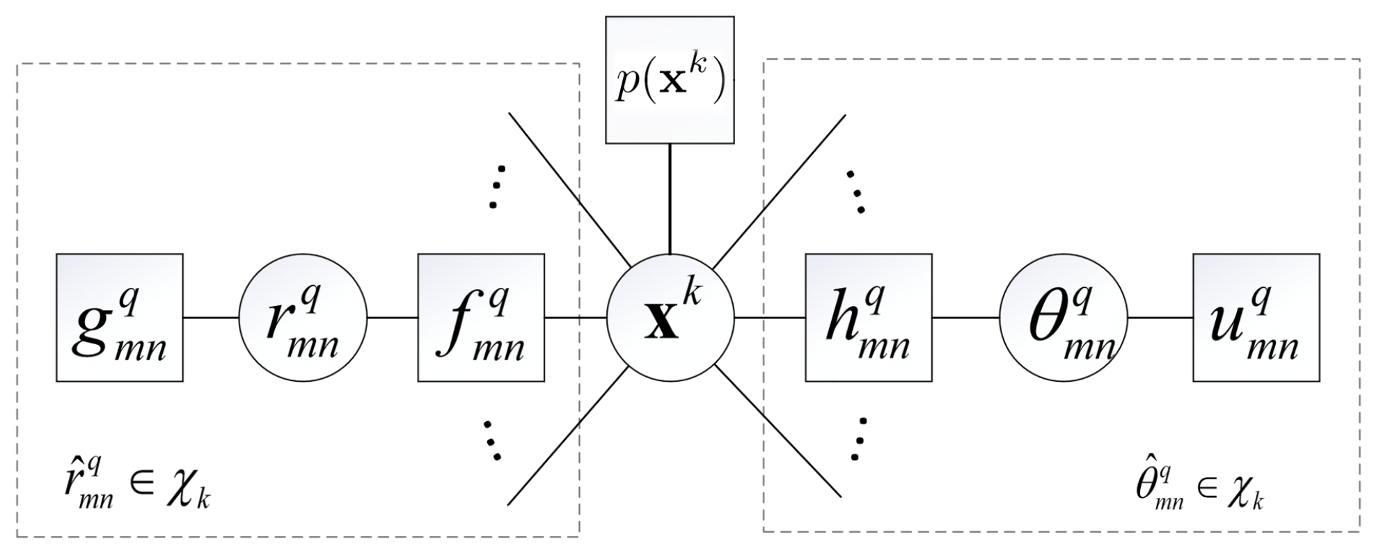
Thus far, we have factorized the optimization problem (19) as a product of multiple local functions. We employ a circle to represent a variable node and a square to represent a function node. By connecting variable nodes with their corresponding function nodes, we can obtain the factor graph representation of (7), as illustrated in Figure 1. Note that we omit the variables of the functions for the convenience of notation.
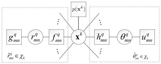
Figure 1.
Factor graph representation of (19).
The factor graph shown in Figure 1 illustrates the factorization of the optimization problem. There are three kinds of branches connected to the central node : the BR observation branches (left side), the AOA observation branches (right side), and the target location prior at the top. To achieve inference on the factor graph, we need to calculated messages in two directions: from factor nodes to variable nodes and from variable nodes to factor nodes, both of which can be efficiently derived using the sum-product algorithm (SPA) framework [35]. Due to the complexity of (19), it is still intractable to find to maximize it. However, the factor graph in Figure 1 provides us with a possible way to find an approximation of , denoted by , which is expected to be easily calculated and maximized. Next, we will utilize message-passing techniques to find .
2.3.2. Message-Passing Algorithm Design
It is observed from Figure 1 that the factor graph has a central variable node with messages flowing from both BR and AOA observation branches towards this central node. For such a factor graph model, the most reasonable message-passing schedule is that messages are passed from two types of branches and fused at the central node : one encompasses BR observation branches (the left half of Figure 1) and the other encompasses AOA observation branches (the right half of Figure 1).
Based on the established factor graph, the belief of can be given by
where denotes the message passed from Node A to Node B, which is a function of . In the following, for these two kinds of branches, we will take and as examples, respectively, to derive the message computations, and those for others can be carried out similarly in parallel.
(1) Message Calculation for BR Observation Branches: For the BR observation branch, based on the Gaussian error model in (5) and the SPA [35], the message from the factor node to the variable node reads
where denotes a Gaussian distribution of x with mean m and variance V.
Based on the structure of the factor graph, we observe that the variable node is connected to two factor nodes and . According to the principles of belief propagation and the SPA, it is not hard to obtain that the outgoing message from to is equivalent to the message , i.e.,
According to the SPA [35], the message can be calculated by the product of and , followed by an integral over , i.e.,
However, the nonlinear function makes unable to be calculated analytically. Although a numerical calculation can be applied to calculate it, it will suffer from a high computation cost and will make the subsequent message calculation intractable. Since is in the Gaussian form, in (23) will remain Gaussian if implies a linear relationship between and . Inspired by extended Kalman filtering [36], we use an iterative message-passing scheme to approximate , i.e., we expand with a first-order Taylor expansion at the estimate of . Then, can be approximated by
where
Note that in (25) and (26) is initialized to the location of the corresponding cluster center for the first iteration. In subsequent iterations, it adopts the estimated value obtained from the last iteration. Leveraging the iterative process, can be dynamically approximated, with the approximation error decreasing gradually. After approximating with , it is not hard to show that
where the weight matrix and mean vector can be calculated directly by the Gaussian message-passing rules [26] with a closed-form, i.e.,
and
So far, we have calculated the BR messages , which are Gaussian functions. Next, we derive the AOA messages in a similar way.
(2) Message Calculation for AOA Observation Branches: Based on the Gaussian error model (6), the message from to can be expressed by
According to the structure of the factor graph, the message is forwarded to , i.e.,
Then, based on SPA, it is not hard to show that can be calculated by the product of and , followed by an integral over , i.e.,
To tackle the above nonlinear integral, we use the same technique to approximate , i.e., we expand at the estimate of , which leads to
where
Note that in (34) and (35) is initialized to the location of the corresponding cluster center for the first iteration, and it adopts the estimated value obtained from the last iteration in subsequent iterations. Using the linear approximation in (33), the message in (32) can be approximated by
with its weight matrix and mean vector being given by
and
Up until now, we have derived the messages of BR and AOA observation branches, both of which are Gaussian functions. Since the product of Gaussian functions is still Gaussian, the in (20) remains Gaussian, i.e., , where and are, respectively, given by [26]
and
Thanks to the Gaussian form of , it can be easily maximized at its mean , i.e., the estimate of is . The proposed localization algorithm is summarized in Algorithm 2.
| Algorithm 2 Target location refinement with message passing. |
|
2.3.3. Complexity Analysis
In this subsection, we analyze the complexity of the proposed method. For Algorithm 1, we first need to calculate all EPs by the closed form solution (8) and their corresponding NDSs by (13). Note that these can be performed in parallel and that the computational complexity of this step is proportional to . After that, we need to calculate the distance between each pair of EPs, with the computational complexity being proportional to . Subsequently, we sequentially perform K searches to obtain K cluster centers, with the complexity of each search and the computational complexity of this step being proportional to . For Algorithm 2, the computation complexity per iteration is dominated by (39) and (40). Note that although matrix inversion is involved in (40), is a small (only 2 × 2) matrix, so the mean and variance of each message can be obtained through linear complexity addition and multiplication operations efficiently. Moreover, the computation complexity per iteration for each target is proportional to . Overall, the computation complexity of the proposed method is proportional to . To the best of our knowledge, this is the first work investigating data-level multi-target association and localization with range and angle measurements in distributed radars. Thus, we cannot make a comparison with existing methods. From the perspective of existing state-of-the-art single-target localization approaches [17,18], their complexity is proportional to due to matrix inversion operations, being significantly higher than our message-passing-based single-target localization method .
3. Results
In this section, extensive Monte Carlo simulations are conducted to verify the performance of the proposed method. We consider a MIMO radar system with transmitters located at m, m, m, m, and m, and receivers located at m, m, m, m, and m. Multiple targets are arranged in an evenly spaced manner on a circle with a radius R and centered at the origin.
Given that both and are inversely proportional to the SNR, there exists a linear relationship between and . In our simulation, we set . Following [16,17,18] and without the loss of generality, we further assume that both and are identical for each observation channel. Additionally, the detection probability for each channel is formulated as , where denotes the complementary error function and denotes the probability of a false alarm [37]. Note that the false alarm rate is typically set to between to . In our simulation, we set the of each observation channel to . Thus, the false alarm rate of overall system will still be much lower than . The iteration process is limited to a maximum of 15 cycles, and target location convergence is deemed achieved when the residual falls below 0.001 m.
We consider an EP as accurately associated if it is correctly matched to a target or correctly identified as a false alarm. The average association accuracy rate is denoted by . Furthermore, is used to denote the probability that a normal EP is misclassified as a false alarm, and represents the probability of correctly identifying the number of targets. The target localization performance is evaluated using the RMSE, which is defined as , where is the estimate of for the lth trial and is the number of trials. To the best of our knowledge, multi-target localization with BR and AOA measurements in distributed radars has not been adequately studied. Therefore, we compare our clustering-based measurement association method with four well-known clustering algorithms, including K-means [38], Mahalanobis distance-based K-means [39], DBSCAN [40] and GMM-based clustering [41]. After that, we employ the proposed method to perform measurement association and then compare the RMSE performance of the proposed method with state-of-the-art algorithms, including the convex solution [17] and algebraic solution [18].
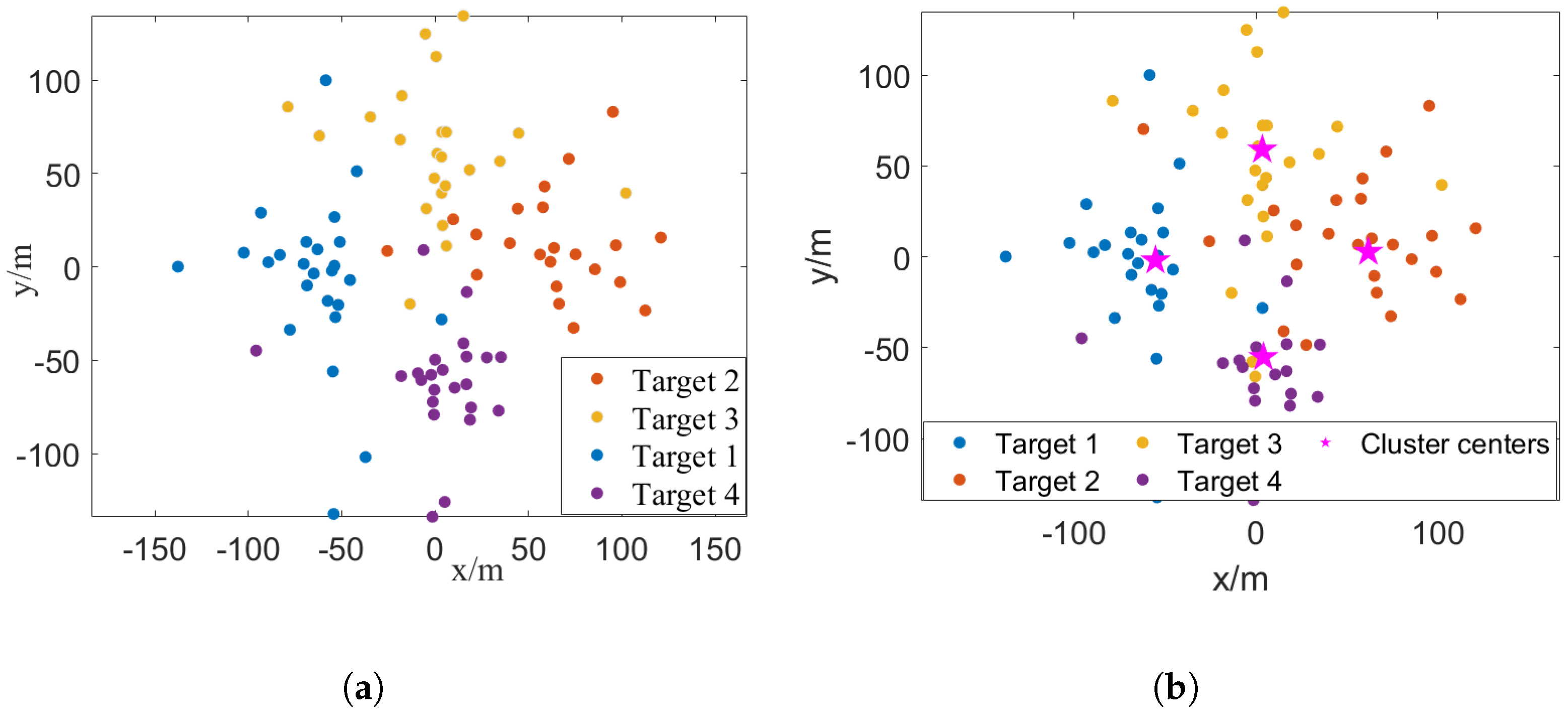
Scenario 1: We first investigate the localization performance under different SNRs, where the corresponding SNRs, and are listed in Table 1. Consider a scenario with four targets arranged at equal angular intervals around a circular path of radius R = 60 m centered at the origin. We first take a specific example in the case of SNR = 10 dB and illustrate the distribution of EPs and corresponding association results in Figure 2a and Figure 2b, respectively. In this specific example, it is noteworthy that the proposed method attains a remarkable association accuracy = 94%, even when EPs from different targets are somewhat mixed and intuitively difficult to cluster.

Table 1.
The SNR range and corresponding and .
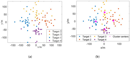
Figure 2.
A specific example of the distribution of EPs and the association results in Scenario 1, where SNR = 10 dB, , R = 60 m. (a) The distribution of EPs. (b) The association results in this specific example, where the proposed measurement association method achieves .
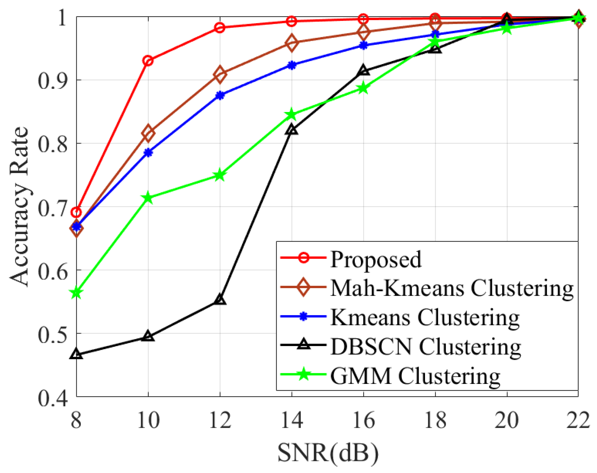
In Figure 3, our investigation of the association performance under different SNRs is illustrated. As observed in Figure 3, the proposed method exhibits significantly higher accuracy compared to directly adopting [38,39,40,41]. The results also demonstrate the effectiveness of the utilized distance metric and the designed set of neighboring EPs. Additionally, in Table 2, we present the probability of identifying a normal EP as a false alarm, denoted by , as well as the probability of correctly identifying the number of targets, denoted by , across different SNR levels. It is demonstrated that remains at a very small value and gradually decreases with an increasing SNR. Moreover, the proposed method can accurately identify K under different SNR levels.
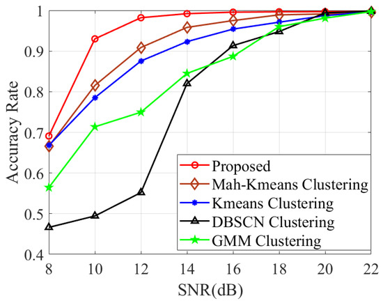
Figure 3.
Association accuracy comparison of various methods with varying SNRs.
Table 2.
The probabilities and under different SNR levels in Scenario 1.
In Figure 4, we compare the localization performance of the proposed method with the convex solution [17] and algebraic solution [18]. Since these methods do not account for a multi-target case, we first employ the proposed method to perform measurement association and then compare the RMSE of different methods. Notably, the proposed method demonstrated superior localization accuracy compared to [17,18], particularly in low-SNR conditions. It is also evident that the localization results from the second stage exhibit notably smaller errors than those of the clustering centers obtained in the first stage.
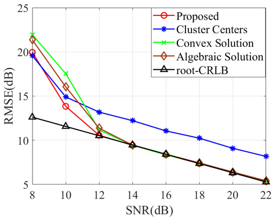
Figure 4.
RMSE comparison of various methods with varying SNRs.
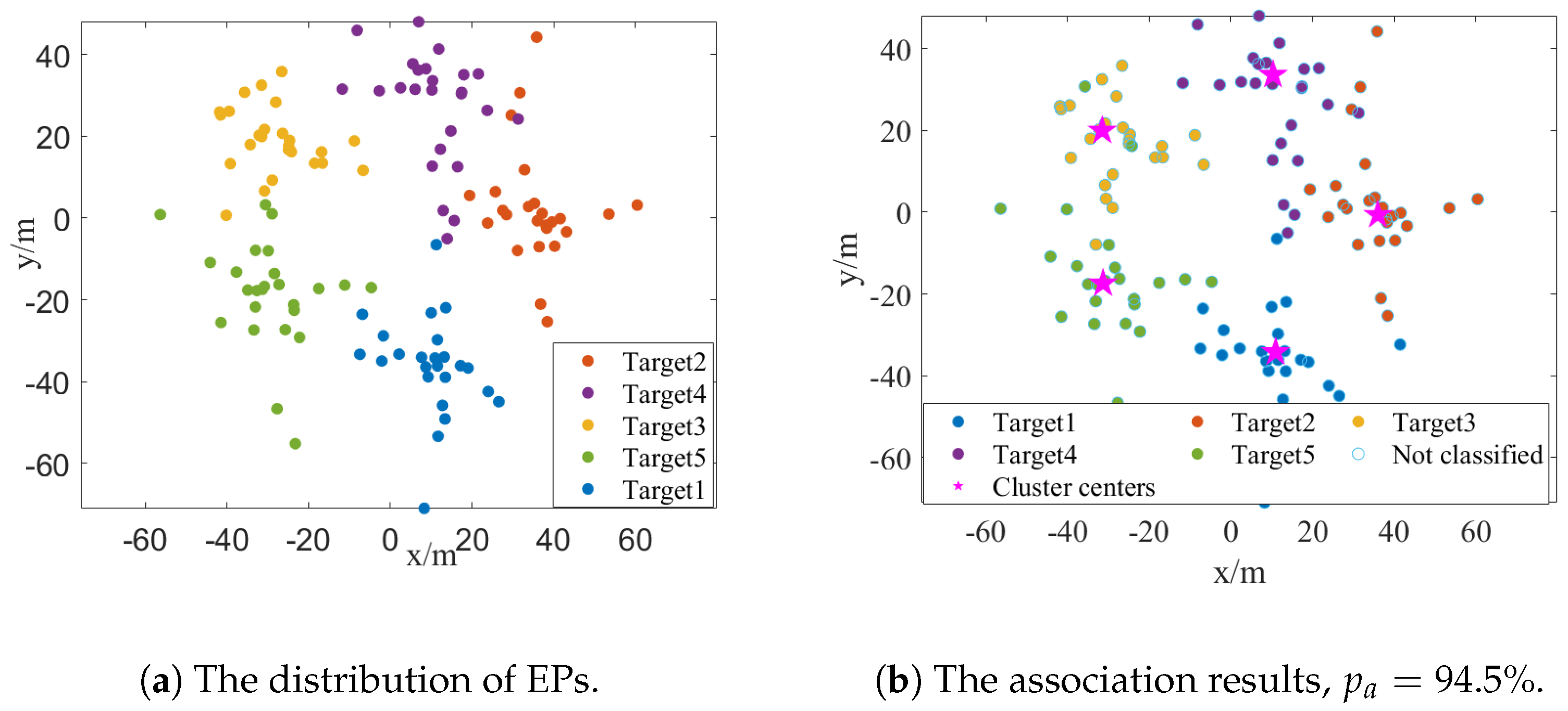
Scenario 2: In the second scenario, we investigate the impact of target spacing on measurement association and target localization performance. Specifically, we set the SNR to 18 dB and arrange five targets uniformly distributed along a circular, with radii R varying from 25 m to 95 m. We also first present an illustrative example of the distribution of the EPs and the association results where R is 35 m, as depicted in Figure 5a and Figure 5b, respectively. Despite the noticeable overlap among the EPs of different targets, the proposed clustering method still attains an impressive association accuracy of 94.5% in this specific example.
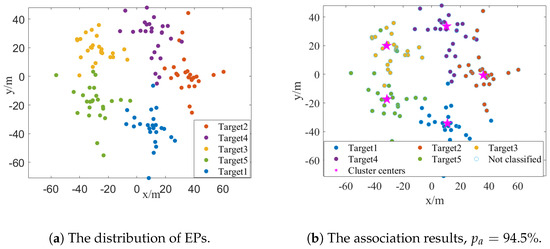
Figure 5.
A specific example of the distribution of EPs and the association results in Scenario 2, where SNR = 18 dB, , R = 35 m. (a) The distribution of EPs. (b) The association results in this specific example, where the proposed measurement association method achieves .
The comparison of measurement association accuracy across different target spacings is presented in Figure 6. It is apparent that the proposed method significantly surpasses other clustering methods, achieving nearly 100% accuracy when the radius R exceeds 55 m. In Table 3, we present and across different R values. It is shown that gradually declines as target spacing increases. Additionally, the proposed clustering algorithm demonstrates a remarkable ability to correctly identify the number of targets K, with an accuracy of 99.4% when R = 25 m.
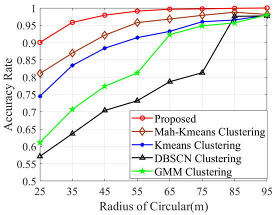
Figure 6.
Association accuracy comparison of various methods with varying radii R.
Table 3.
The probabilities and under different R in Scenario 2.
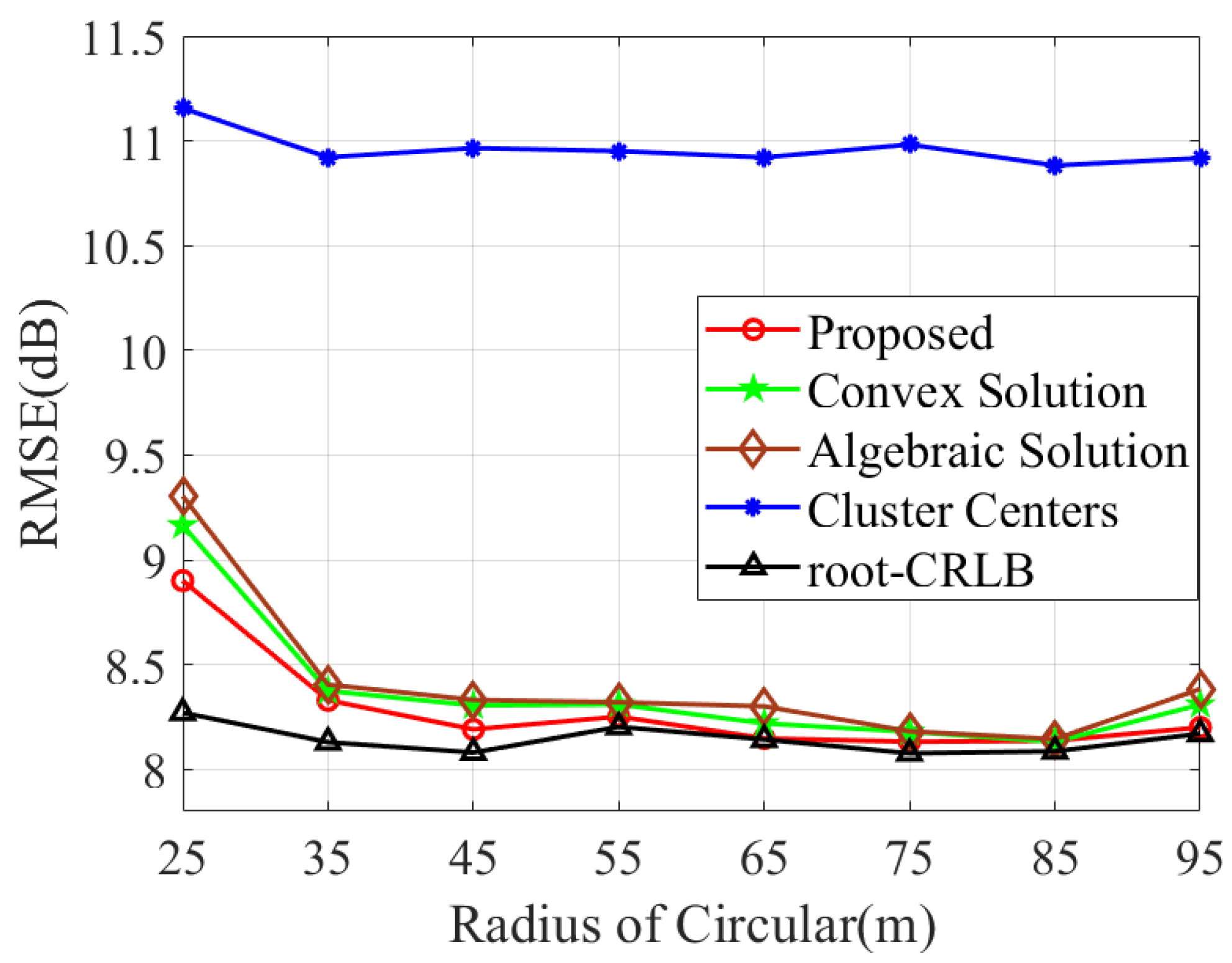
Furthermore, we apply the proposed method to accomplish measurement association and compare the RMSE performance with [17,18]. As illustrated in Figure 7, the proposed method outperforms [17,18], and it also exhibits a superior consistency with CRLB over a broad range of target spacings.
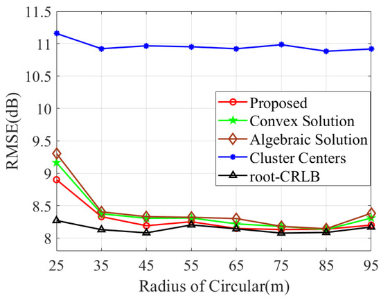
Figure 7.
RMSE comparison of various methods with varying target distribution radii R.
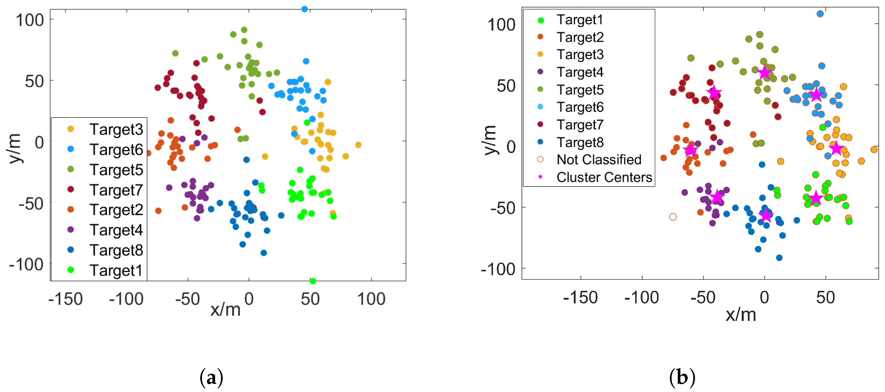
Scenario 3: In the third scenario, we investigate the impact of the number of targets K on localization performance. We set the radius R to 60 m, the SNR to 16 dB, and gradually increase K from 3 to 9. Taking the case of eight targets as an example, we depict the distribution of the EPs and the results after clustering in Figure 8a and Figure 8b, respectively. It can be observed that the EPs corresponding to different targets no longer have clear boundaries and are difficult to separate visually. However, even in this scenario, the proposed method still attains a association accuracy of 95.2%, demonstrating its robustness and effectiveness.

Figure 8.
A specific example of the distribution of EPs and the association results in Scenario 3, where SNR = 16 dB and K = 8, m. (a) The distribution of EPs. (b) The association results in this specific example, where the proposed measurement association achieves . The pink stars represent the cluster centers obtained by the proposed method.
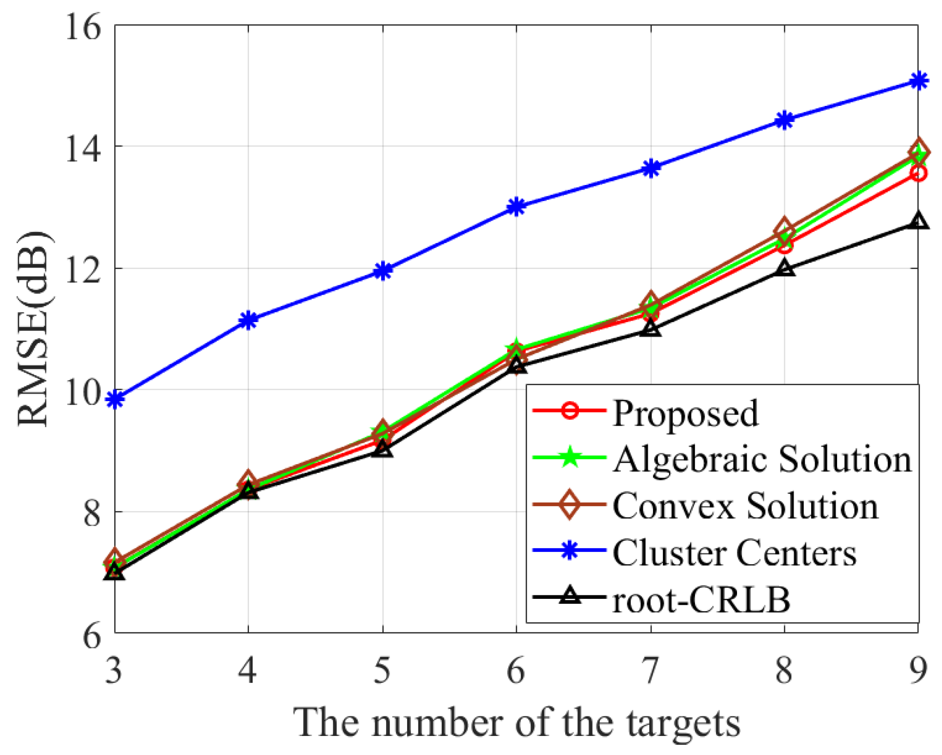
The comparison of association accuracy among different methods is illustrated in Figure 9. It can be observed that the association accuracy of the proposed method is notably higher than that of [38,39,40,41]. In Table 4, we present and across K. It is shown that gradually increases as K increases. Additionally, the proposed clustering algorithm is capable of accurately identifying the exact target number when . Lastly, the RMSE of target location across varying numbers of targets is presented in Figure 10. It can be seen that the proposed algorithm outperforms both [17,18] in terms of the RMSE across different target counts while achieving a closer approximation to the CRLB.
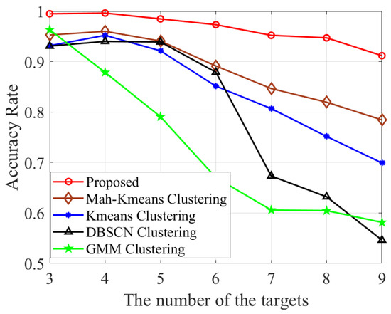
Figure 9.
Association accuracy comparison of various methods with varying K.
Table 4.
The probabilities and for varying number of targets K in Scenario 3.
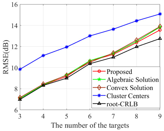
Figure 10.
RMSE comparison of various methods with varying target distribution radii R.
At the end of this section, to clearly illustrate the characteristics and performance of different algorithms, we provide a comparison in Table 5 to quickly grasp the advantages of the proposed approach compared to existing techniques.
Table 5.
Comparison of different methods for multi-target localization.
4. Discussion
The simulation results presented in this study demonstrate several important findings regarding measurement association and target localization in distributed MIMO radar systems. The proposed two-stage approach consistently outperformed traditional clustering methods and state-of-the-art localization algorithms across various scenarios involving closely spaced targets.
The clustering-based measurement association method exhibited remarkable robustness, achieving high accuracy even in challenging conditions. Specifically, the method maintained superior performance when targets were closely spaced (e.g., radius R = 35 m), when the number of targets increased, and when operating at lower SNR levels. This robust performance can be attributed to the careful definition of distance metrics and neighboring EP sets, which effectively handle both false alarms and missed detections. The probability of correctly identifying the target number also remained consistently high across different scenarios, demonstrating its practical reliability. Our approach successfully maintained the association accuracy above 90% in most test cases, while competitive methods showed significant degradation as conditions worsened.
From a localization perspective, the message-passing algorithm demonstrated excellent consistency with the CRLB over a wider range of conditions compared to existing methods. The algorithm dynamically approximated complex local functions, proving particularly effective in reducing the computational complexity while maintaining high accuracy. This computational efficiency is particularly valuable for real-time applications. Additionally, our approach showed greater resilience to low-SNR conditions, a critical advantage in practical radar systems where signal quality may vary.
These findings suggest that the proposed method offers a promising solution to the challenging problem of closely spaced multi-target localization in distributed MIMO radar systems. These findings suggest that the capability of the proposed method to maintain high performance across various operational conditions while minimizing computational requirements makes it particularly suitable for practical deployments in various applications, such as formation target tracking, where targets may be closely spaced and accurate localization is essential.
5. Conclusions
In this work, we have presented an efficient multi-target localization method with BR and AOA measurements. We first transformed the intractable measurement association problem into a clustering problem. Then, we developed an efficient clustering approach. After that, we applied the factor graph techniques for single-target localization. The iterative message-passing strategy was adopted to dynamically approximate the complex local factors, leading to high localization accuracy while maintaining low complexity. Extensive simulation results demonstrated that the proposed method can achieve efficient measurement association and localization for closely spaced targets for missed alarms and false alarms. It also should be noted that the performance of our approach may be affected when the SNR is particularly low or when the number of targets in a given area is high. Furthermore, our approach relies on the multi-channel structure of receivers for AOA measurements and assumes Gaussian measurement errors, which may not always hold in practice. Future work could focus on extending the proposed framework to accommodate non-Gaussian error distributions, developing techniques that function with limited measurement types, and enhancing the robustness of the proposed approach in challenging environments.
Author Contributions
Conceptualization, Z.Y.; methodology Z.Y. and Q.G.; formal analysis, Z.Y.; software, Z.Y. and Z.J.; writing—original draft preparation, Z.Y. and Z.J.; investigation, T.S.; validation, T.S.; supervision, J.D., J.L. and Q.G. All authors have read and agreed to the published version of the manuscript.
Funding
This research was funded by the National Natural Science Foundation of China (grant numbers 62401438 and 62171350).
Data Availability Statement
The raw data supporting the conclusions of this article will be made available by the authors on request.
Conflicts of Interest
The authors declare no conflicts of interest.
Appendix A. The Solution of (8)
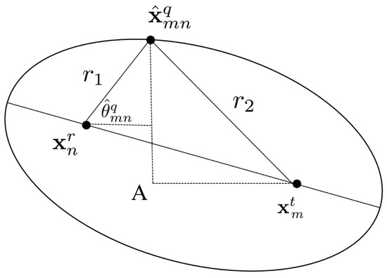
Figure A1.
The illustration of the solution of (8).
Figure A1.
The illustration of the solution of (8).
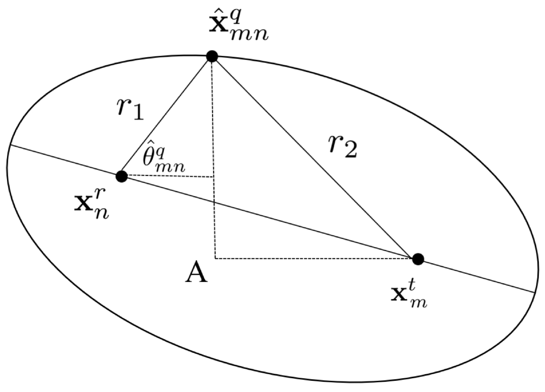
In this appendix, we derive the closed-form solution of (8). As shown in Figure A1, we denote , and . The horizontal line (parallel to the x-axis) passing through intersects with the vertical line (parallel to the y-axis) passing through at point A. It is clear that . In the triangle , according to the Pythagorean theorem, we have
By squaring both sides of (A1) and performing some polynomial calculations, we can obtain
Then, it is not hart to obtain
Appendix B. The Derivation of the CRLB of
In this appendix, we derive the CRLB of an EP . Based on the BR and AOA measurements’ pair and the Gaussian noise model, the CRLB of is given by
where is the Fisher information matrix (FIM). It is calculated by
where
and
References
- Chen, P.; Zheng, L.; Wang, X.; Li, H.; Wu, L. Moving Target Detection Using Colocated MIMO Radar on Multiple Distributed Moving Platforms. IEEE Trans. Signal Process. 2017, 65, 4670–4683. [Google Scholar] [CrossRef]
- Yu, Z.; Li, J.; Guo, Q.; Ding, J. Efficient Direct Target Localization for Distributed MIMO Radar with Expectation Propagation and Belief Propagation. IEEE Trans. Signal Process. 2021, 69, 4055–4068. [Google Scholar] [CrossRef]
- Zhao, H.; Zhang, Z.; Chen, Z.; Fan, H.; Lv, Z.; Bi, J. A Multiple-Input Multiple-Output Synthetic Aperture Radar Echo Separation and Range Ambiguity Suppression Processing Framework for High-Resolution Wide-Swath Imaging. Remote Sens. 2025, 17, 609. [Google Scholar] [CrossRef]
- Li, H.; Wang, Z.; Liu, J.; Himed, B. Moving Target Detection in Distributed MIMO Radar on Moving Platforms. IEEE J. Sel. Top. Signal Process. 2015, 9, 1524–1535. [Google Scholar] [CrossRef]
- Liu, H.; Li, Y.; Cheng, W.; Dong, L.; Yan, B. Sensing-Efficient Transmit Beamforming for ISAC with MIMO Radar and MU-MIMO Communication. Remote Sens. 2024, 16, 3028. [Google Scholar] [CrossRef]
- He, Q.; Blum, R.S.; Haimovich, A.M. Noncoherent MIMO Radar for Location and Velocity Estimation: More Antennas Means Better Performance. IEEE Trans. Signal Process. 2010, 58, 3661–3680. [Google Scholar] [CrossRef]
- Abtahi, A.; Azghani, M.; Marvasti, F. An Adaptive Iterative Thresholding Algorithm for Distributed MIMO Radars. IEEE Trans. Aerosp. Electron. Syst. 2019, 55, 523–533. [Google Scholar] [CrossRef]
- Zhou, J.; Li, H.; Cui, W. Low-Complexity Joint Transmit and Receive Beamforming for MIMO Radar with Multi-Targets. IEEE Signal Process. Lett. 2020, 27, 1410–1414. [Google Scholar] [CrossRef]
- Liang, J.; Wang, D.; Su, L.; Chen, B.; Chen, H.; So, H.C. Robust MIMO radar target localization via nonconvex optimization. Signal Process. 2016, 122, 33–38. [Google Scholar] [CrossRef]
- Liang, J.; Chen, Y.; So, H.C.; Jing, Y. Circular/hyperbolic/elliptic localization via Euclidean norm elimination. Signal Process. 2018, 148, 102–113. [Google Scholar] [CrossRef]
- Nguyen, N.H.; Dogancay, K. Closed-Form Algebraic Solutions for 3-D Doppler-Only Source Localization. IEEE Trans. Wirel. Commun. 2018, 17, 6822–6836. [Google Scholar] [CrossRef]
- Wielgo, M.; Krysik, P.; Misiurewicz, J.; Kulpa, K. Doppler-only localization problem solution for PCL radar. In Proceedings of the 2015 16th International Radar Symposium (IRS), Dresden, Germany, 24–26 June 2015; pp. 60–64. [Google Scholar]
- Chen, X.; Wang, G.; Ho, K. Semidefinite Relaxation Method for Unified Near-Field and Far-Field Localization by AOA. Signal Process. 2021, 181, 107916. [Google Scholar] [CrossRef]
- Wang, G.; Ho, K.C.; Chen, X. Bias Reduced Semidefinite Relaxation Method for 3-D Rigid Body Localization Using AOA. IEEE Trans. Signal Process. 2021, 69, 3415–3430. [Google Scholar] [CrossRef]
- Amiri, R.; Behnia, F.; Noroozi, A. Efficient Joint Moving Target and Antenna Localization in Distributed MIMO Radars. IEEE Trans. Wirel. Commun. 2019, 18, 4425–4435. [Google Scholar] [CrossRef]
- Amiri, R.; Behnia, F.; Zamani, H. Efficient 3-D Positioning Using Time-Delay and AOA Measurements in MIMO Radar Systems. IEEE Commun. Lett. 2017, 21, 2614–2617. [Google Scholar] [CrossRef]
- Kazemi, S.A.R.; Amiri, R.; Behnia, F. Efficient Convex Solution for 3-D Localization in MIMO Radars Using Delay and Angle Measurements. IEEE Commun. Lett. 2019, 23, 2219–2223. [Google Scholar] [CrossRef]
- Kazemi, S.A.R.; Amiri, R.; Behnia, F. Efficient Closed-Form Solution for 3-D Hybrid Localization in Multistatic Radars. IEEE Trans. Aerosp. Electron. Syst. 2021, 57, 3886–3895. [Google Scholar] [CrossRef]
- Jabbari, M.R.; Taban, M.R.; Gazor, S. A robust TSWLS localization of moving target in widely separated MIMO radars. IEEE Trans. Aerosp. Electron. Syst. 2022, 59, 897–906. [Google Scholar] [CrossRef]
- Jabbari, M.R.; Taban, M.R.; Gazor, S.; Kaimasi, M. Asymptotically Efficient Moving Target Localization in Distributed Radar Networks. IEEE Trans. Signal Inf. Process. Over Netw. 2023, 9, 569–580. [Google Scholar] [CrossRef]
- Song, H.; Wen, G.; Liang, Y.; Zhu, L.; Luo, D. Target Localization and Clock Refinement in Distributed MIMO Radar Systems with Time Synchronization Errors. IEEE Trans. Signal Process. 2021, 69, 3088–3103. [Google Scholar] [CrossRef]
- Kazemi, S.A.R.; Amiri, R.; Behnia, F. Data Association for Multi-Target Elliptic Localization in Distributed MIMO Radars. IEEE Commun. Lett. 2021, 25, 2904–2907. [Google Scholar] [CrossRef]
- Kang, S.; Shin, H.; Chung, W. A novel geometric-based bistatic range grouping algorithm for multi-target localization in distributed MIMO radar systems. Expert Syst. Appl. 2024, 253, 124269. [Google Scholar] [CrossRef]
- Zhu, L.; Wen, G.; Liang, Y.; Luo, D.; Jian, H. Multitarget enumeration and localization in distributed MIMO radar based on energy modeling and compressive sensing. IEEE Trans. Aerosp. Electron. Syst. 2023, 59, 4493–4510. [Google Scholar] [CrossRef]
- Zhou, Q.; Yuan, Y.; Venturino, L.; Yi, W. Direct Target Localization for Distributed Passive Radars with Direct-Path Interference Suppression. IEEE Trans. Signal Process. 2024, 72, 3611–3625. [Google Scholar] [CrossRef]
- Loeliger, H. An introduction to factor graphs. IEEE Signal Process. Mag. 2004, 21, 28–41. [Google Scholar] [CrossRef]
- Loeliger, H.; Dauwels, J.; Hu, J.; Korl, S.; Ping, L.; Kschischang, F.R. The Factor Graph Approach to Model-Based Signal Processing. Proc. IEEE 2007, 95, 1295–1322. [Google Scholar] [CrossRef]
- Haimovich, A.M.; Blum, R.S.; Cimini, L.J. MIMO Radar with Widely Separated Antennas. IEEE Signal Process. Mag. 2008, 25, 116–129. [Google Scholar] [CrossRef]
- Amiri, R.; Behnia, F.; Maleki Sadr, M.A. Efficient Positioning in MIMO Radars with Widely Separated Antennas. IEEE Commun. Lett. 2017, 21, 1569–1572. [Google Scholar] [CrossRef]
- Ma, F.; Guo, F.; Yang, L. Low-complexity TDOA and FDOA localization: A compromise between two-step and DPD methods. Digit. Signal Process. 2020, 96, 102600. [Google Scholar] [CrossRef]
- Skolnik, M.I. Radar Handbook, 3rd ed.; McGraw-Hill: New York, NY, USA, 2008. [Google Scholar]
- Panwar, K.; Babu, P.; Stoica, P. Maximum likelihood algorithm for time-delay based multistatic target localization. IEEE Signal Process. Lett. 2022, 29, 847–851. [Google Scholar] [CrossRef]
- De Maesschalck, R.; Jouan-Rimbaud, D.; Massart, D.L. The mahalanobis distance. Chemom. Intell. Lab. Syst. 2000, 50, 1–18. [Google Scholar] [CrossRef]
- Grafarend, E.W. Linear and Nonlinear Models: Fixed Effects, Random Effects, and Mixed Models; de Gruyter: Vienna, Austria, 2006. [Google Scholar]
- Kschischang, F.R.; Frey, B.J.; Loeliger, H. Factor graphs and the sum-product algorithm. IEEE Trans. Inf. Theory 2001, 47, 498–519. [Google Scholar] [CrossRef]
- Julier, S.J.; Uhlmann, J.K. Unscented filtering and nonlinear estimation. Proc. IEEE 2004, 92, 401–422. [Google Scholar] [CrossRef]
- Mahafza, B.R. Radar Systems Analysis and Design Using MATLAB; Chapman and Hall/CRC: Boca Raton, FL, USA, 2005. [Google Scholar]
- Hartigan, J.A.; Wong, M.A. A k-means clustering algorithm. Appl. Stat. 1979, 28, 100–108. [Google Scholar] [CrossRef]
- Brown, P.O.; Chiang, M.C.; Guo, S.; Jin, Y.; Leung, C.K.; Murray, E.L.; Pazdor, A.G.; Cuzzocrea, A. Mahalanobis distance based k-means clustering. In Proceedings of the International Conference on Big Data Analytics and Knowledge Discovery, Vienna, Austria, 22–24 August 2022; Springer: Cham, Switzerland, 2022; pp. 256–262. [Google Scholar]
- Ester, M.; Kriegel, H.P.; Sander, J.; Xu, X. A density-based algorithm for discovering clusters in large spatial databases with noise. In Proceedings of the KDD, Portland, OR, USA, 2–4 August 1996; Volume 96, pp. 226–231. [Google Scholar]
- Shanmugam, R. Finite Mixture Models. Technometrics 2002, 44, 82. [Google Scholar] [CrossRef]


Disclaimer/Publisher’s Note: The statements, opinions and data contained in all publications are solely those of the individual author(s) and contributor(s) and not of MDPI and/or the editor(s). MDPI and/or the editor(s) disclaim responsibility for any injury to people or property resulting from any ideas, methods, instructions or products referred to in the content. |
© 2025 by the authors. Licensee MDPI, Basel, Switzerland. This article is an open access article distributed under the terms and conditions of the Creative Commons Attribution (CC BY) license (https://creativecommons.org/licenses/by/4.0/).