An Automated Framework for Interaction Analysis of Driving Factors on Soil Salinization in Central Asia and Western China

Abstract

Soil salinization is a global ecological and environmental problem, which is particularly serious in arid areas. The formation process of soil salinity is complex, and the interactive effects of natural causes and anthropogenic activities on soil salinization are elusive. Therefore, we propose an automated machine learning framework for predicting soil salt content (SSC), which can search for the optimal model without human intervention. At the same time, post hoc interpretation methods and graph theory knowledge are introduced to visualize the nonlinear interactions of variables related to SSC. The proposed method shows robust and adaptive performance in two typical arid regions (Central Asia and Xinjiang Province in western China) under different environmental conditions. The optimal algorithms for the Central Asia and Xinjiang regions are Extremely Randomized Trees (ET) and eXtreme Gradient Boosting (XGBoost), respectively. Moreover, precipitation and minimum air temperature are important feature variables for salt-affected soils in Central Asia and Xinjiang, and their strongest interaction effects are latitude and normalized difference water index. In both study areas, meteorological factors exhibit the greatest effect on SSC, and demonstrate strong spatiotemporal interactions. Soil salinization intensifies with long-term climate warming. Regions with severe SSC variation are mainly distributed around the irrigation water source and in low-terrain basins. From 1950 to 2100, the regional mean SSC (g/kg) varies by +20.94% and +64.76% under extreme scenarios in Central Asia and Xinjiang, respectively. In conclusion, our study provides a novel automated approach for interaction analysis of driving factors on soil salinization in drylands.

1. Introduction

Soil salinization is a global ecological and environmental problem [1,2,3]. It refers to the process by which salts from deep soil or groundwater are transported to the surface through capillary action, and the salts accumulate on the soil surface after evaporation [4,5]. Salt-affected soils hinder plant growth and occur globally, especially in drylands [6]. According to the Global Map of Salt-Affected Soils released by the Food and Agriculture Organization of the United Nations (FAO), the area of global soil salinization is over 1381 Mha (10.7 percent of the total area of the earth). A total of 7.4 percent of land in Asia is affected, including 94 Mha in Kazakhstan, 41 Mha in Uzbekistan, and 36 Mha in China [7]. Soil salinization is caused by natural environmental factors (e.g., scarce precipitation, intense evaporation, and a high groundwater table) and human activities (e.g., excessive water use due to irrigation and grazing activities, and the improper application of fertilizers) [6,7,8,9,10,11,12]. It has been proved that salt moves with water [13,14]. In recent years, global warming has significantly affected the terrestrial water cycle, leading to increasingly severe soil salinization [15,16]. Salt-affected soils not only contribute to soil degradation but also poses a significant threat to global food security and the balance of ecosystems [10,17]. Therefore, investigations of the spatiotemporal variations and underlying driving mechanisms of soil salinization hold substantial strategic and practical importance for safeguarding agricultural productivity and achieving sustainable development [13,18].

The complex nature of soil salinity formation makes its dynamic monitoring a challenging task [2,19]. Traditional methods, which integrate field sampling with laboratory simulation, tend to be time-intensive and laborious [20,21]. Consequently, numerical simulation models have become an essential tool for quantitatively studying soil salinity. Models such as HYDRUS, SWAP, DRAINMOD, and SWAT, which are based on solute transport mechanisms in unsaturated soils, rely on clear physical principles to capture realistic dynamic changes in soil salinity [22,23,24]. However, the nonlinear behavior of water movement in unsaturated soils increases the complexity of model parameters, thereby limiting the applicability of these numerical approaches in large-scale regions [1,25,26].

With the transition from data scarcity to data abundance, artificial intelligence technology has garnered significant attention in the realms of remote sensing and eco-geography [27]. Digital Soil Mapping (DSM) has emerged as a novel and efficient approach for representing the spatial distribution of soils [28,29]. At the same time, remote sensing technology, leveraging its long-term Earth observation capabilities, provides a comprehensive and diverse dataset for large-scale soil salinity mapping [3,11]. Data-driven machine learning methods, with their advantages of processing high-dimensional data and capturing nonlinear relationships, are extensively applied in DSM [18,20]. Several studies have compared the effectiveness of various data-driven algorithms in mapping soil properties, such as Support Vector Machine, neural network, and tree-based models, and the performance of the models varies across different studies [23,30,31,32]. It has been proved that the selection of appropriate algorithms and the fine-tuning of hyperparameters are crucial steps in enhancing the performance of machine learning models [32,33,34]. It is challenging to establish a fixed model that is universally applicable across all scenarios [35,36]. Currently, most research relies on semi-automated machine learning approaches, where the modeling process still requires substantial manual involvement. For example, this process requires the user to (1) manually adjust the multiple parameters of a single model, and (2) make multiple modeling approaches based on various algorithms, with the performance meticulously debugged through iterative comparison and experimentation. Such semi-automated methods make it difficult to achieve the dynamic updating of the model, and have poor transferability for studies with spatiotemporal heterogeneity. Therefore, to avoid the influence of human subjective factors on the results, it is crucial to explore fully automated and adaptive soil salinity prediction models.

The SCORPAN model stands as the predominant framework in DSM, rooted in the Dokuchaev–Jenny principle that soil properties are the result of the interactions among soil-forming factors over time [28,37]. The SCORPAN framework suggests that soil characteristics are influenced by the environmental factors of soil, climate, organisms, relief (terrain attributes), parent material, age (time of the soil), and spatial position [29,37]. Soil salinity is a key issue in the soil–plant–atmosphere system [16,26]. The performances of this relationship vary with different environmental conditions [15,33,38]. To reveal the interactive relationship between soil salinity and environmental variables, early studies mainly used a statistical analysis method, such as Pearson correlation analysis, linear regression, and geographically weighted regression [19]. These statistical methods have the advantages of simple modeling, easy implementation, and high efficiency, but they can only describe the linear correlation among various factors [33,39]. Machine learning can capture the nonlinear relationship between variables, but as a black box model, its results are difficult to intuitively represent. In 2017, the Defense Advanced Research Projects Agency released the Explainable Artificial Intelligence program, which aims to enable users to better understand, trust, and effectively manage artificial intelligence [40,41]. In this context, several post hoc interpretation algorithms are widely employed, such as the SHapley Additive explanation (SHAP) [42], Local Interpretable Model-Agnostic Explanations (LIME) [43], and Partial Dependence Plots (PDP) [44], etc. Therefore, combining machine learning models with post hoc interpretation algorithms to visualize the interaction between research objects and relevant factors is a hot topic in the eco-geographic field.

In this paper, we propose an automated framework for interaction analysis of driving factors on soil salinization. Our contribution is as follows: (a) building an SSC prediction model that can automatically search for the best combination of algorithm, hyperparameters, and features; (b) visualizing the nonlinear interactions between variables related to the SSC based on the model interpretation method and graph theory knowledge; and (c) using long-term climate change factors as driven data to explore the spatial and temporal variation of SSC under different scenarios from 1950 to 2100. In summary, the whole workflow of our study can be seen in Figure 1.

2. Materials and Methods

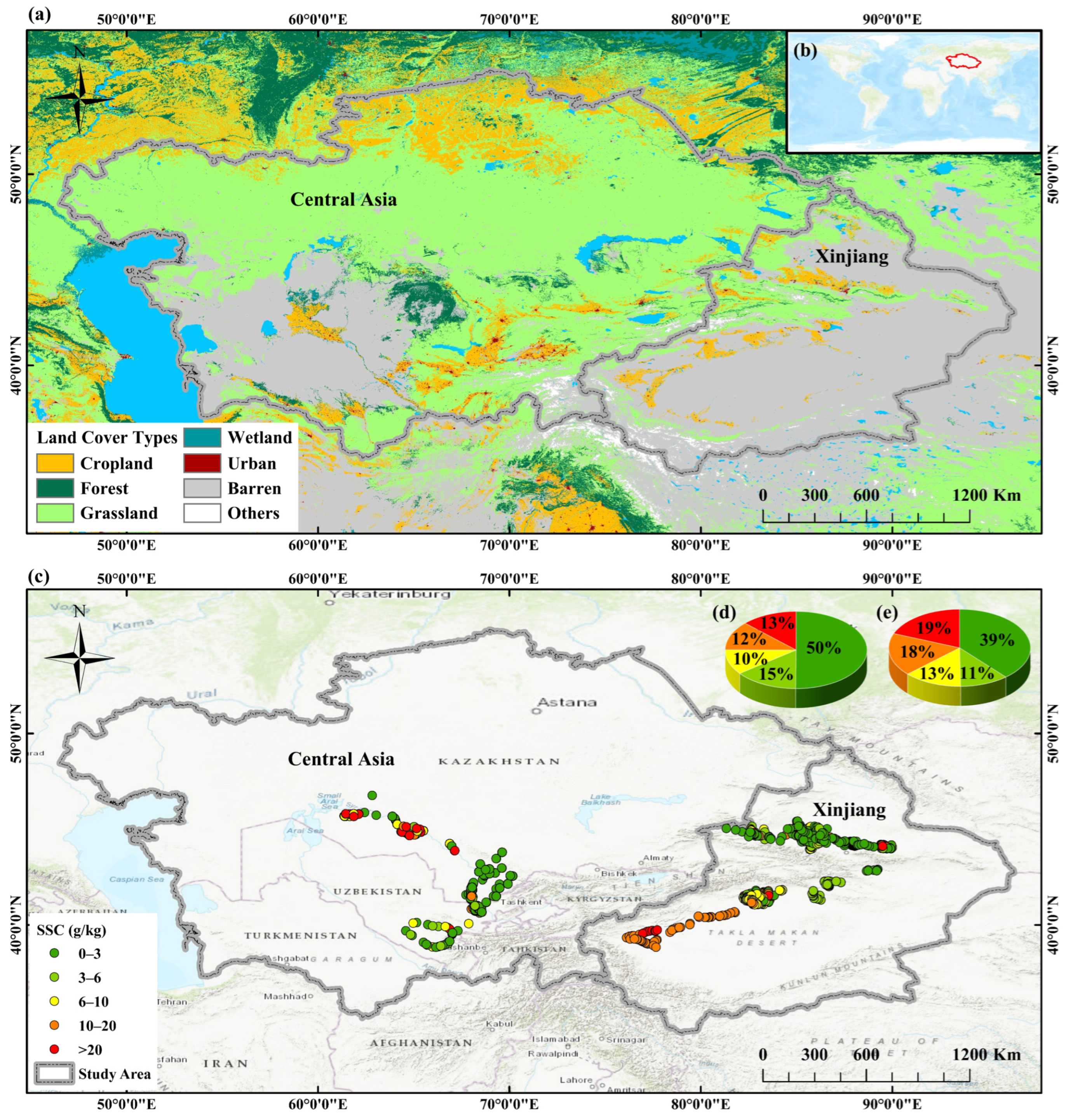
2.1. Study Areas

Central Asia (35°N to 55°N and 46°E to 87°E, Figure 2) comprises five countries—Kazakhstan, Kyrgyzstan, Tajikistan, Uzbekistan, and Turkmenistan—located in the middle of the Eurasian continent [45]. It boasts a unique geographical position, particularly with its southeastern high mountains blocking the warm and moist air currents from the Indian and Pacific Oceans, resulting in an arid, high-temperature, and continental climate in the region. In most areas, the annual precipitation is below 300 mm, with high evaporation rates of approximately 1500–2000 mm/year [46]. Summers are hot, with temperatures reaching above 40 °C, while winters are cold, with minimum temperatures dropping below −20 °C [46,47]. The Aral Sea basin, the Ob Basin, and the Balkhash Basin are the important water systems in Central Asia [48].

Xinjiang (34°N to 49°N and 73°E to 96°E, Figure 2), located in the northwest of China, holds a significant position in the Silk Road Economic Belt. With the Altai Mountains on the north boundary and the Kunlun Mountains on the south boundary, the Tianshan Mountains in the middle divide Xinjiang into two parts, North Xinjiang and South Xinjiang [49]. To the north of the Tianshan Mountains lies China’s second-largest basin, the Junggar Basin, and to the south is the world’s largest inland basin, the Tarim Basin. The region experiences a typical arid continental climate, with an average annual precipitation of about 150 mm (less than 50 mm in the Tarim Basin) and an evaporation rate as high as 2000–3000 mm/year [4,8,50]. The diurnal temperature variation is significant, and the region enjoys long sunshine hours, with annual sunshine duration ranging from approximately 2500 to 3500 h [51].

Central Asia and Xinjiang are typical drylands which have an arid climate and limited water resources [21,36]. The land cover mainly includes croplands, grasslands, forests, bare areas, snow and ice, water bodies, and urban areas. This vulnerable environment seriously restricts the development of the local economy and society [14,52]. Due to the influence of natural conditions and human activities, the soil salination phenomenon is common in Central Asia and Xinjiang [17,19].

2.2. Ground Sampling Data Acquisition

In this paper, the observed values of SSC were obtained by field investigation from 2008 to 2018. The specific sampling process was as follows: (1) make routes in advance, and try to select diverse soil types to ensure that the samples were representative of the regional characteristics. (2) Three topsoil samples (the soil depth was approximately 20 cm) were randomly selected near the site, and mixed into one bag. The geographic location of each site was recorded using the hand-held GPS device. (3) The soil samples brought back to the laboratory were air-dried, ground, and sifted with a 2 mm sifter. The total soil salt content was finally measured based on the 1:5 soil–water extraction solution. The sampling points were primarily located in the oasis croplands along the Syr Darya and Amu Darya rivers in Central Asia (518 samples) and at the foothills of the Tianshan Mountains in Xinjiang (978 samples). The spatial distribution of the samples in the study areas is shown in Figure 2c. It can be seen from the statistics (Figure 2d,e) that non-saline soil (SSC < 3 g/kg) has the highest proportion in Central Asia and Xinjiang, while the proportion of extremely saline soil (SSC > 20 g/kg) in Xinjiang is higher than that in Central Asia.

2.3. Environmental Variable Extraction

Based on the formation conditions of soil salinization in the soil–plant–atmosphere system, six groups of 37 environmental variables were extracted in our study, including spatiotemporal indicator, meteorological factor, vegetation index, topographic factor, soil factor, and human activity indicator (

Table 1. Information of salinization-related predictor variable.

Group	Feature	Source	Temporal/Spatial Resolution
Spatiotemporal Indicator	Year, Latitude (Lat), Longitude (Lon)	Field Investigation	—
Meteorological Factor	Mean Air Temperature (Tmean)	GEE ‘NASA/GDDP-CMIP6’	daily/0.25°
	Maximum Air Temperature (Tmax)	ditto	ditto
	Minimum Air Temperature (Tmin)	ditto	ditto
	Precipitation (Prcp)	ditto	ditto
	Wind Speed (WindS)	ditto	ditto
	Relative Humidity (RH)	ditto	ditto
	Specific Humidity (SH)	ditto	ditto
	Vapor Pressure Deficit (VPD)	$6.108 \times {\mathrm{e}}^{{\displaystyle \frac{17.27\times \mathrm{Ta\_mean}}{\mathrm{Ta\_mean}+273.3}}}\times \left(1-\mathrm{RH}\right)$	ditto
	Evapotranspiration (ET)	GEE ‘NASA/FLDAS/NOAH01/C/GL/M/V001’	monthly/0.1°
Vegetation Index	Normalized Difference Vegetation Index (NDVI)	(NIR − Red)/(NIR + Red)	daily/500 m
	Enhanced Vegetation Index (EVI)	2.5 × ((NIR − Red)/(NIR + 6 × Red − 7.5 × Blue + 1))	ditto
	Normalized Difference Water Index (NDWI)	(Green − NIR)/(Green + NIR)	ditto
	Land Surface Water Index (LSWI)	(NIR − SWIR1)/(NIR + SWIR1)	ditto
	Leaf Area Index (LAI)	GEE ‘MODIS/061/MCD15A3H’	4-day/500 m
	Fraction of Photosynthetically Active Radiation (FPAR)	ditto	ditto
	Standardized Precipitation Evapotranspiration Index (SPEI)	GEE ‘CSIC/SPEI/2_9’	monthly/0.5°
Topographic Factor	Elevation, Slope, Aspect, Roughness	GEE ‘USGS/SRTMGL1_003’	Static/30 m
Soil Factor	Soil Moisture (SM)	GEE ‘NASA/FLDAS/NOAH01/C/GL/M/V001’	daily/0.1°
	Soil Temperature (Tsoil)	ditto	ditto
	Soil Bulk Density (Bulk)	Harmonized World Soil Database	static/1 km
	Soil Texture (Texture)	ditto	ditto
	Soil pH (PH)	ditto	ditto
	Soil Organic Carbon (SOC)	ditto	ditto
	Soil Clay Fraction (Clay)	ditto	ditto
	Soil Sand Fraction (Sand)	ditto	ditto
	Soil Silt Fraction (Silt)	ditto	ditto
Human Activity Indicator	Land-use/Land-cover (LULC)	GEE ‘MODIS/061/MCD12Q1’	yearly/500 m
	Global Livestock Distribution (Livestock)	FAO Livestock Systems	static/5 arc-minutes
	Cultivated Area (CA)	World Bank Open Data	Statistic
	Per Capita GDP (GDP)	ditto	ditto
	Population Density (Population)	ditto	ditto

). Google Earth Engine (GEE) is a comprehensive cloud platform with a large number of data resources, big data processing tools, and high-performance computing capabilities [18,39]. In this paper, multi-source remote sensing data were obtained based on the GEE platform, including the images from the NASA Earth Exchange Global Daily Downscaled dataset (NEX-GDDP-CMIP6), ERA5-Land reanalysis dataset, MODIS collections products, Landsat surface reflectance dataset, FLDAS dataset, SPEI database, and Digital Elevation Model.

The NEX-GDDP-CMIP6 dataset contains historical and future projections for 1950–2100 based on output from CMIP6 [53,54]. Additionally, several variables from three greenhouse gas emissions scenarios known as Shared Socioeconomic Pathways (SSPs) (historical, SSP2-4.5, and SSP5-8.5) are provided from thirty-four global climate models [54]. The bias-correction spatial disaggregation (BCSD) technique was utilized to downscale the dataset to a resolution of 0.25° [55,56]. Based on the average of thirty-four global climate models provided by the NEX-GDDP-CMIP6 dataset, mean air temperature (Tmean), maximum air temperature (Tmax), minimum air temperature (Tmin), precipitation (Prcp), wind speed (WindS), relative humidity (RH), specific humidity (SH), and vapor pressure deficit (VPD) were selected as meteorological factors. In this study, evapotranspiration (ET) provided by the FLDAS dataset is considered as a meteorological variable. The FLDAS dataset also provides the soil moisture (SM) and soil temperature (Tsoil) data. The NDVI, EVI, NDWI, and LSWI were calculated using established formulas applied to the Moderate Resolution Imaging Spectroradiometer (MODIS) surface reflectance images (MOD09GA) with cloud cover of less than 20%. Leaf Area Index (LAI) and Fraction of Photosynthetically Active Radiation (FPAR) were provided by the MCD15A3H product. The Global SPEI database (SPEIbase) offers robust long-time information about drought conditions at the global scale, with a 0.5° pixel size and monthly cadence. The topographic factors were derived from the Shuttle Radar Topography Mission (SRTM), and several soil factors were sourced from the Harmonized World Soil Database (HWSD).

Human activities have progressively intensified in both scope and magnitude, significantly influencing land-use and land-cover (LULC) changes [45,56]. Livestock grazing is a significant and widespread LULC practice in drylands [57]. LULC changes and overgrazing have a major impact on soil salinization [58,59]. Therefore, this study incorporates factors related to human activities, encompassing LULC, livestock distribution, cultivated area, and socioeconomic indicators such as per capita GDP and population density. Global LULC maps were obtained from the MODIS Land Cover Type product (MCD12Q1), and were reclassified into seven classes: cropland, forests, grassland, wetland, building, desert, and others. The Gridded Livestock of the World (GLW) was published by the FAO, which includes the global livestock distributions of sheep, goats, cattle, buffaloes, horses, pigs, chickens, and ducks [60]. Different types of data were synthesized into comprehensive livestock maps according to the conversion criteria released by the Ministry of Agriculture and Rural Affairs, PRC: 1 goat $\approx$ 0.9 sheep, 1 cattle $\approx$ 6 sheep, 1 buffalo $\approx$ 6.6 sheep, 1 horse $\approx$ 6 sheep, 1 pig $\approx$ 2 sheep, 1 chicken $\approx$ 0.05 sheep, and 1 duck $\approx$ 0.05 sheep. The World Bank Open Data website provides open access global statistic data. We linked the obtained statistics to the global vector map, and then converted the vector layer into the GeoTIFF files.

Finally, all the acquired data were processed on the GEE platform. Prcp and ET were processed as annual sums, and all other variables were processed as annual averages. To ensure data consistency, a spatial resolution of 500 m was chosen when constructing the training feature set sampled from remote sensing images.

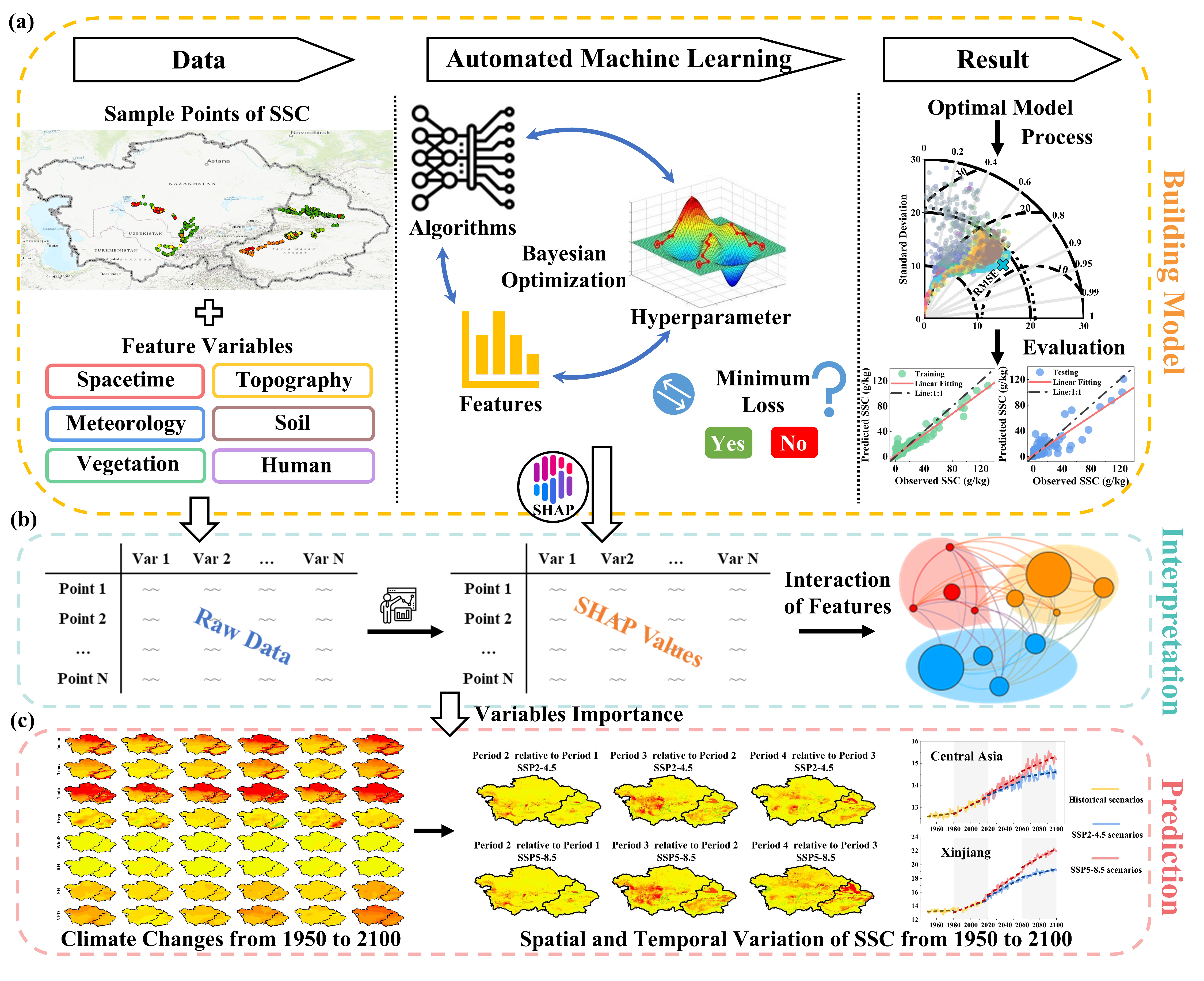
2.4. Automated Soil Salinization Prediction Model

In machine learning, different combinations of algorithms and hyperparameters will affect the model performance. An automated model can be realized by using machine learning instead of manual methods to complete decisions made in the modeling process. Bayesian optimization is an algorithm for parameter optimization based on prior information [61]. Compared with the methods such as random search, grid search, and particle swarm optimization, the Bayesian optimization algorithm can find the global optimal solution within fewer iterations [27,34]. Therefore, this paper proposes an automated soil salinization prediction model which achieves the joint optimization of algorithms and hyperparameters in the Bayesian optimization framework. The objective of this study is to rapidly iterate among multiple models through an automated process and select the optimal model based on the characteristics of the input data. The proposed model can try multiple algorithms simultaneously in a single trial and find the optimal combination of the algorithm and its hyperparameters by minimizing the objective function (Figure 1a). Twelve models were selected from the python package: Elastic Net, Support Vector Machine (SVM), K-Nearest Neighbor (KNN), Decision Tree (DT), Random Forest (RF), Extremely Randomized Trees (ET), Adaptive Boosting (AdaBoost), Gradient Boosting Decision Tree (GBDT), eXtreme Gradient Boosting (XGBoost), Light Gradient Boosting Machine (LightGBM), Categorical Boosting (CatBoost), and Multilayer Perceptron (MLP). The models and their hyperparameters are shown in

Table 2. Information of selected models and their hyperparameters.

Model	Hyperparameters
Elastic Net	alpha, L1_ratio
Support Vector Machine	C, kernel
K-Nearest Neighbor	n_neighbors, weights, p
Decision Tree	max_depth, min_samples_leaf, min_samples_split, max_features
Random Forest	n_estimators, max_depth, max_leaf_nodes, min_samples_leaf, min_samples_split, max_features
Extremely Randomized Trees	n_estimators, max_depth, min_samples_leaf, min_samples_split, max_features
Adaptive Boosting	n_estimators, learning_rate, loss
Gradient Boosting Decision Tree	n_estimators, subsample, max_depth, learning_rate, min_samples_leaf, min_samples_split, max_features
eXtreme Gradient Boosting	n_estimators, subsample, max_depth, learning_rate, colsample_bytree, gamma, reg_alpha, reg_lambda
Light Gradient Boosting Machine	num_leaves, n_estimators, subsample, max_depth, learning_rate, colsample_bytree, min_child_weight, min_child_samples, reg_alpha, reg_lambda
Categorical Boosting	subsample, learning_rate, l2_leaf_reg, colsample_bylevel, depth, min_data_in_leaf, one_hot_max_size
Multilayer Perceptron	hidden_layer_sizes, activation, alpha, learning_rate, learning_rate_init

, and the hyperparameter configuration space during the modeling process is provided in the Table S1.

2.5. Relationship Analysis Between SSC and Environmental Variables

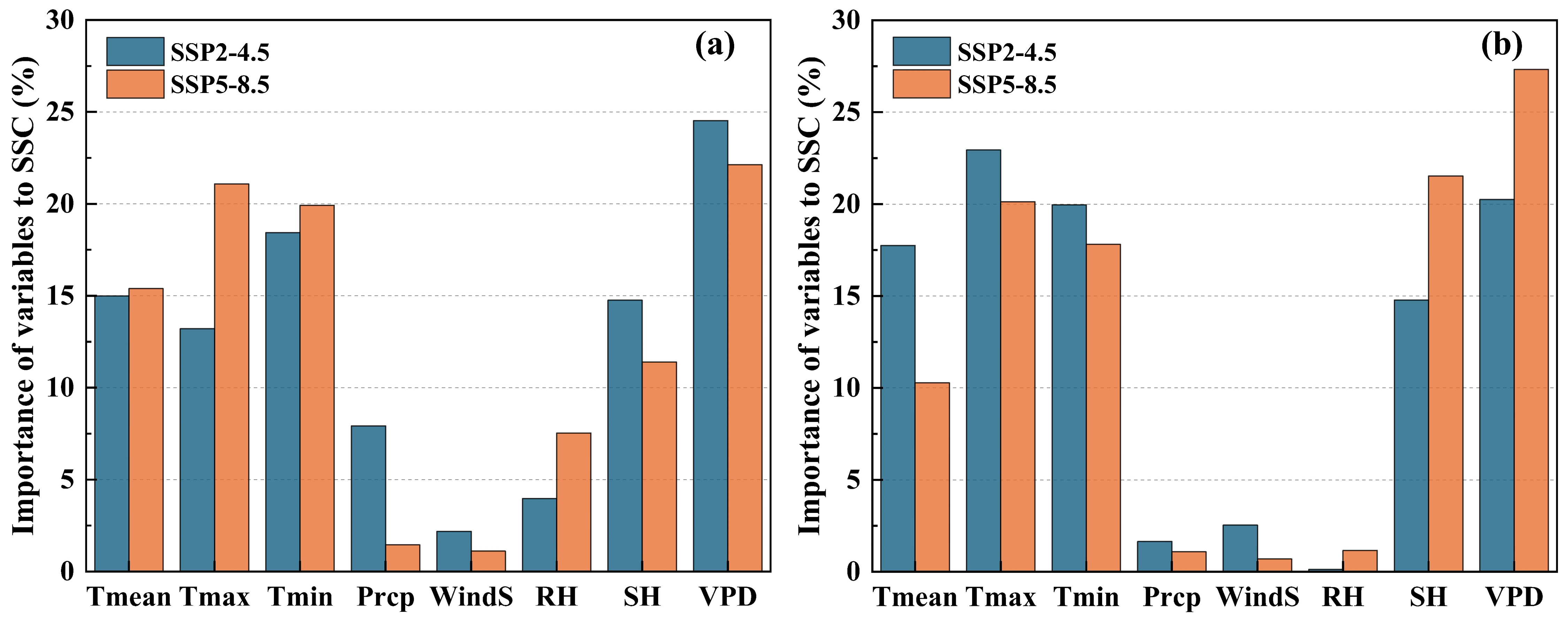
2.5.1. Model Interpretation Based on the Post Hoc Interpretation Algorithm

The SHAP originates from game theory, and it is a post hoc interpretation algorithm that can explain the prediction process and feature importance of machine learning models [42,62]. Compared with other algorithms, the SHAP provides model interpretation from both local and global perspectives [42]. Therefore, a combination of the automated machine learning model and the SHAP algorithm can effectively identify key features and explore the interactive relationship between the variables (Figure 1b). The feature set composed of environmental variables related to SSC is denoted as $\mathrm{M}=\left\{{\mathrm{x}}_{1,}{\mathrm{x}}_{2, \dots ,}{\mathrm{x}}_{\mathrm{m}}\right\}$, and m is the number of features. The SHAP value of feature ${\mathrm{x}}_{\mathrm{i}}$ can be expressed as,

$$\mathrm{SHAP}\left({\mathrm{x}}_{\mathrm{i}}\right)=\sum _{\mathrm{S}\subseteq \left\{{\mathrm{x}}_{1,}{\mathrm{x}}_{2, \dots ,}{\mathrm{x}}_{\mathrm{m}}\right\}\backslash \left\{{\mathrm{x}}_{\mathrm{i}}\right\}}{\displaystyle \frac{\left|\mathrm{S}\right|!\left(\mathrm{m}-\left|\mathrm{S}\right|-1\right)!}{\mathrm{m}!}}\times \left[\mathrm{f}\left(\mathrm{S}\cup \left\{{\mathrm{x}}_{\mathrm{i}}\right\}\right)-\mathrm{f}\left(\mathrm{S}\right)\right]$$

(1)

where S represents an arbitrary subset excluding ${\mathrm{x}}_{\mathrm{i}}$, and $\left|\mathrm{S}\right|$ is the size of the subset S; $\mathrm{f}\left(\mathrm{S}\right)$ is the output of the model corresponding to the subset S, and $\mathrm{f}\left(\mathrm{S}\cup \left\{{\mathrm{x}}_{\mathrm{i}}\right\}\right)$ is the output of the model corresponding to the set that adds ${\mathrm{x}}_{\mathrm{i}}$ into the subset S. Features with a larger sum of absolute SHAP values have more impact on the predicted value of the model [63]. Moreover, SHAP interaction values were developed to describe the contributions of features in terms of their main effects and interaction effects [41,63].

$$\mathrm{SHAP}\left({\mathrm{x}}_{\mathrm{i},\mathrm{j}}\right)={\sum }_{\mathrm{S}\subseteq \left\{{\mathrm{x}}_{1,}{\mathrm{x}}_{2, \dots ,}{\mathrm{x}}_{\mathrm{m}}\right\}\backslash \left\{{\mathrm{x}}_{\mathrm{i}},{\mathrm{x}}_{\mathrm{ij}}\right\}}{\displaystyle \frac{\left|\mathrm{T}\right|!\left(\mathrm{m}-\left|\mathrm{T}\right|-2\right)!}{\mathrm{m}!}}\times \left[\mathrm{f}\left(\mathrm{T}\cup \left\{{\mathrm{x}}_{\mathrm{i}},{\mathrm{x}}_{\mathrm{j}}\right\}\right)-\mathrm{f}\left(\mathrm{T}\cup \left\{{\mathrm{x}}_{\mathrm{i}}\right\}\right)-\mathrm{f}\left(\mathrm{T}\cup \left\{{\mathrm{x}}_{\mathrm{j}}\right\}\right)+\mathrm{f}\left(\mathrm{T}\right)\right]$$

(2)

$$\mathrm{SHAP}\left({\mathrm{x}}_{\mathrm{i},\mathrm{i}}\right)=\mathrm{SHAP}\left({\mathrm{x}}_{\mathrm{i}}\right)-\sum _{\mathrm{j}\ne \mathrm{i}}\mathrm{SHAP}\left({\mathrm{x}}_{\mathrm{i},\mathrm{j}}\right)$$

(3)

where $\mathrm{SHAP}\left({\mathrm{x}}_{\mathrm{i},\mathrm{j}}\right)$ represent the SHAP interaction effect of features ${\mathrm{x}}_{\mathrm{i}}$ and ${\mathrm{x}}_{\mathrm{j}}$; T is an arbitrary subset not containing ${\mathrm{x}}_{\mathrm{i}}$ and ${\mathrm{x}}_{\mathrm{j}}$; $\mathrm{f}\left(\mathrm{T}\right)$ is the output of the model corresponding to the subset T; $\mathrm{f}\left(\mathrm{T}\cup \left\{{\mathrm{x}}_{\mathrm{i}}\right\}\right)$, $\mathrm{f}\left(\mathrm{T}\cup \left\{{\mathrm{x}}_{\mathrm{j}}\right\}\right),$ and $\mathrm{f}\left(\mathrm{T}\cup \left\{{\mathrm{x}}_{\mathrm{i}},{\mathrm{x}}_{\mathrm{j}}\right\}\right)$ are the output of the model corresponding to the set that adds ${\mathrm{x}}_{\mathrm{i}}$, ${\mathrm{x}}_{\mathrm{j}}$, and both ${\mathrm{x}}_{\mathrm{i}}$ and ${\mathrm{x}}_{\mathrm{j}}$ into the subset T, respectively; $\mathrm{SHAP}\left({\mathrm{x}}_{\mathrm{i},\mathrm{i}}\right)$ represents the main effect of feature ${\mathrm{x}}_{\mathrm{i}}$.

2.5.2. Correlation Visualization Based on Knowledge Graph

Based on the SHAP, the effect of each group on soil salinization can be further evaluated. However, the intricate relationship between the components limits their visual expression. The knowledge graph describes multiple entities and their relationships in the form of graphs, providing a better way to organize, manage, and utilize huge amounts of information [64]. The quality of the graph visualization depends on the effectiveness of the layout algorithm [65]. In the graph with a better layout, important nodes are more prominent and nodes with high association are closer, enabling users to quickly focus on the required information. The force-directed algorithm is widely used in visualization research, which is simple in principle and easy to implement [66,67]. It is mainly based on the action of mechanical gravity and repulsion to transform the complex network structure into a two-dimensional spatial graph [64,67]. Therefore, ForceAtlas2, a force-directed layout algorithm, was used to visualize the interactive relationship between multiple groups of variables related to soil salinization.

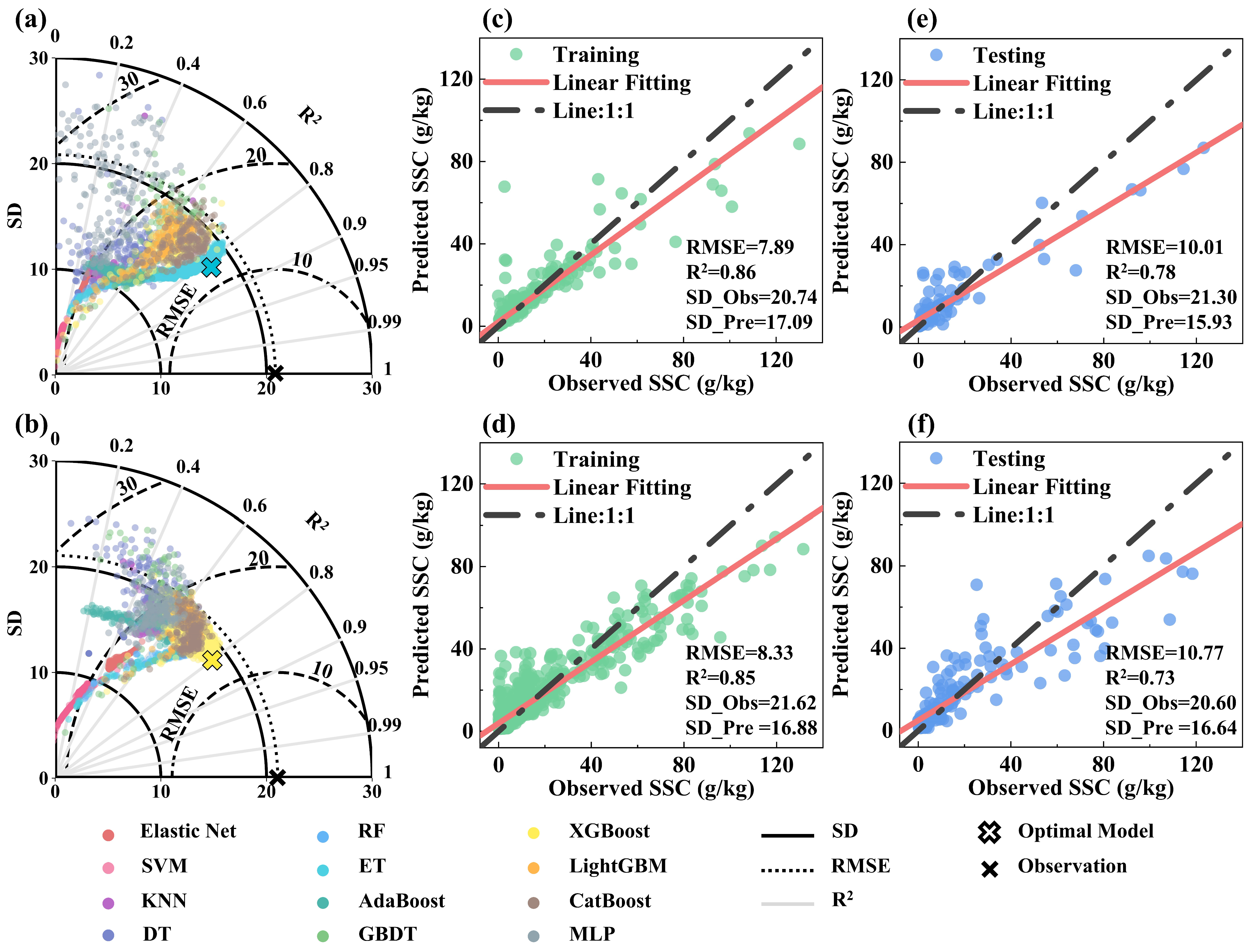
2.6. Model Evaluation

In our study, two statistical metrics were selected to evaluate the accuracy of model prediction, including the root mean square error (RMSE) and determination coefficient (${\mathrm{R}}^2$). The model shows better performance when the RMSE is closer to 0, and the ${\mathrm{R}}^2$ is closer to 1. The formula used to calculate the RMSE and ${\mathrm{R}}^2$ is as follows,

$$\mathrm{RMSE}=\sqrt{{\displaystyle \frac{1}{\mathrm{N}}}\sum _{\mathrm{i}=1}^{\mathrm{N}}{\left({\mathrm{y}}_{\mathrm{i}}-\widehat{{\mathrm{y}}_{\mathrm{i}}}\right)}^2}$$

(4)

$${\mathrm{R}}^2=1-{\displaystyle \frac{\frac{1}{\mathrm{N}}{\sum }_{\mathrm{i}=1}^{\mathrm{N}}{\left({\mathrm{y}}_{\mathrm{i}}-\widehat{{\mathrm{y}}_{\mathrm{i}}}\right)}^2}{\frac{1}{\mathrm{N}}{\sum }_{\mathrm{i}=1}^{\mathrm{N}}{\left({\mathrm{y}}_{\mathrm{i}}-\overline{\mathrm{y}}\right)}^2}}$$

(5)

where N is the number of observations; ${\mathrm{y}}_{\mathrm{i}}$ is the observed value of the SSC; $\widehat{{\mathrm{y}}_{\mathrm{i}}}$ is the predicted SSC of the model; and $\overline{\mathrm{y}}$ is the mean value of the observations. In the experiment, all data were split into 5 folds for cross-validation to avoid model overfitting. The proportion of the training set and the testing set was 4:1.

3. Results

3.1. Accuracy Evaluation of the Automated Model

The algorithm and the hyperparameters jointly affect the results of the model. The proposed model can be automatically updated until the objective function converges. In this paper, the objective function is the mean RMSE of 5-fold cross-validation. The minimum value of the objective function corresponds to the optimal algorithm and the hyperparameter combination. We selected 12 algorithms and conducted a total of 5000 iterations, with each iteration testing a specific algorithm and its hyperparameter combination. The automated optimization process is illustrated in Figure 3a,b. In the figure, each point represents the evaluation result of one experiment, and different algorithms are represented by distinct colors. Within the Bayesian optimization framework, the model consistently progresses towards minimizing the objective value, culminating in the identification of the optimal model within the most densely concentrated region. The optimal models for the Central Asia and Xinjiang regions are ET and XGBoost, respectively, which both have a high R², and the standard deviation (SD) of the model-predicted SSC is close to the observed values. Our results show that the tree-based ensemble learning algorithm performs better than the other algorithms. Furthermore, we evaluated the accuracy of the model on the training and testing sets (Figure 3c–f). According to the sampling points, the soil salinization in the two regions is serious, and the SSC has strong variability. The fitting results show that the optimal models all have an R² that is higher than 0.70 in different scenarios. It indicates that our proposed automated model is robust and adaptive, and performs very well in different study areas.

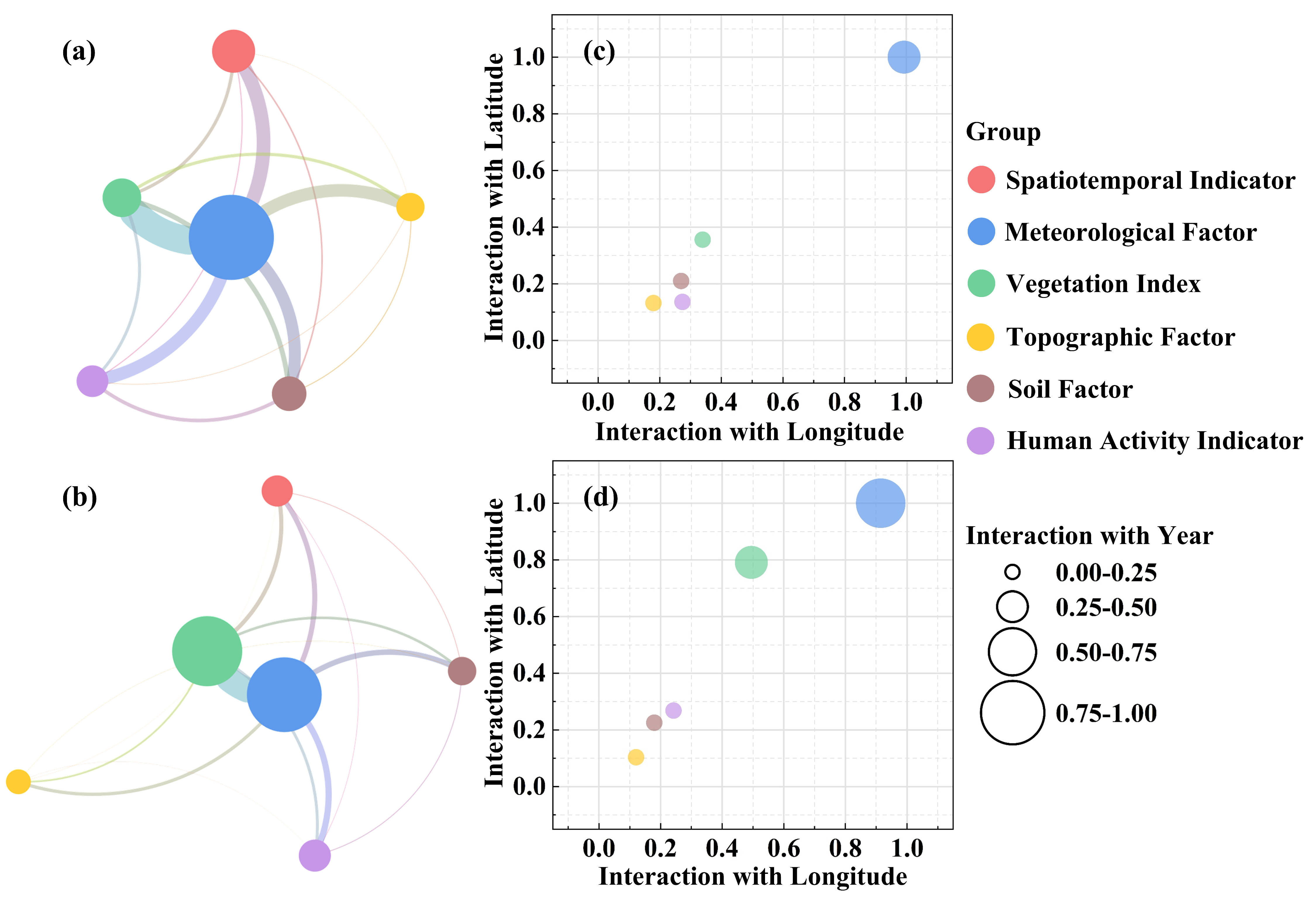
3.2. Interaction Effects Visualization Between the Individual Environmental Variables

In this paper, the contribution of individual features and the interactions between each feature to SSC were calculated using the SHAP value. To facilitate the comparison, we set the sum of the importance of all features and their interactions as 100 percent, and expressed the importance as a percentage. When a feature or interaction with a larger SHAP value appears, this indicates that it has a great positive or negative effect. Figure 4a,b show the top 15 important main effects and their interaction effects in Central Asia and Xinjiang, respectively. The features have a different importance in the two regions, and usually the main effect is larger than its interaction effects. In Central Asia, the top three features that are important to the SSC are Prcp, LULC, and Lat, respectively. While in Xinjiang, the top three important features are Tmin, NDWI, and LSWI, respectively. The interaction dependency graph visualized the nonlinear relationship of features related to SSC. Moreover, it can show the relationship between two features, thus discovering the regularity of the action of a pair of features on SSC. To observe more details of the interaction effect, we plotted an interaction-dependent graph of the most important feature and its strongest interaction effect. The model-predicted value was obtained by summing the average SSC of the training samples and the SHAP values of all its corresponding features. In central Asia, Prcp is the most influential feature on SSC. As the precipitation gradually increases, the SSC gradually decreases (Figure 4c). The cut-off value of the effect of Prcp on SSC is about 200 mm. That is, it promotes the SSC to a level higher than the sample average when Prcp is less than 200 mm, and it suppresses the SSC to a level lower than the sample average when Prcp is greater than 200 mm. Low Prcp is mostly distributed in high latitudes. When the Prcp remains constant, the higher the latitude, the higher the SSC. In Xinjiang, Tmin has the greatest contribution to SSC. Additionally, SSC gradually increases as Tmin increases (Figure 4d). The cut-off value of the effect of Tmin on SSC is about 7 °C. When Tmin is less than 7 °C, it has a positive effect on SSC, and when Tmin is greater than 7 °C, it has a negative effect on SSC. The NDWI index is used to reflect the distribution of water bodies and vegetation, and its values range between −1 and 1. The closer the NDWI of the pixel is to 1, the higher the probability that it is a water body. The closer the NDWI is to −1, the higher the likelihood that the pixel represents vegetation. NDWI values close to 0 indicate that its corresponding pixel is more likely to be bare land. Due to there being fewer water bodies in Xinjiang, the value of the NDWI is mostly negative. When Tmin remains constant, SSC is more sensitive to a high NDWI. That is, the SSC varies significantly in areas with lower water content.

3.3. Interaction Effects Visualization Between the Group Environmental Variables

The interaction between six groups was visualized using the graph layout algorithm. The sum of the importance of all groups and their interaction effect was set as 100 percent. For Central Asia, the layout of the graph is clustered (Figure 5a). The meteorological factor is located at the center of the graph, and all the other groups close toward it. Therefore, the group composed of meteorological factors has the greatest effect on SSC, and it has a strong interaction effect with several other groups. For Xinjiang, the layout of the graph is scattered (Figure 5b). The meteorological factor and vegetation index are located at the center of the graph and the other feature groups are around them. Among them, the topographical factor was the farthest from the other groups. It indicates that the meteorological factor and vegetation index have a large impact on SSC, and there is a significant interaction between them. The topographical factor only interacted with the meteorological factor and vegetation index, and weakly with the other groups. Furthermore, we evaluated the interaction relationships of different feature groups and spatial and temporal indicators (longitude, latitude, and year) (Figure 5c,d). The maximum interaction value was set to 1, and the results were normalized. The results show that the meteorological factor is the strongest spatiotemporal interaction group in both Central Asia and Xinjiang, followed by vegetation index. Additionally, the topographic factor has minimal spatiotemporal interaction. In comparison, the meteorological factor has strong spatial effects in both regions, while it has weaker temporal effects in Central Asia than in Xinjiang. Thus, the effects of meteorological factors on SSC under temporal variations are greater in Xinjiang than in Central Asia.

3.4. Spatiotemporal Variation of SSC in Historical and Future Under Climate Change

According to the importance analysis based on SHAP values, meteorological factors have great effects on SSC in Central Asia and Xinjiang. Multiple studies have shown that climate change may become a major factor affecting soil salinization [32,52], posing significant challenges for soil health and sustainable development in the future. Therefore, we selected the Tmean, Tmax, Tmin, Prcp, WindS, RH, SH, and VPD from 1950 to 2100 provided by CMIP6 as driving data. Based on the feature data in 2020, the automated model was used to explore the spatiotemporal variation of SSC under climate change in historical (1950–2014) and future (2015–2100) periods (Figure 1c). Our results include two scenarios based on the future, SSP2-4.5 and SSP5-8.5 From 1950–2100 is divided into four periods: from 1950 to 1980 is Period 1, from 1981 to 2020 is Period 2, from 2021 to 2060 is Period 3, and from 2061 to 2100 is Period 4.

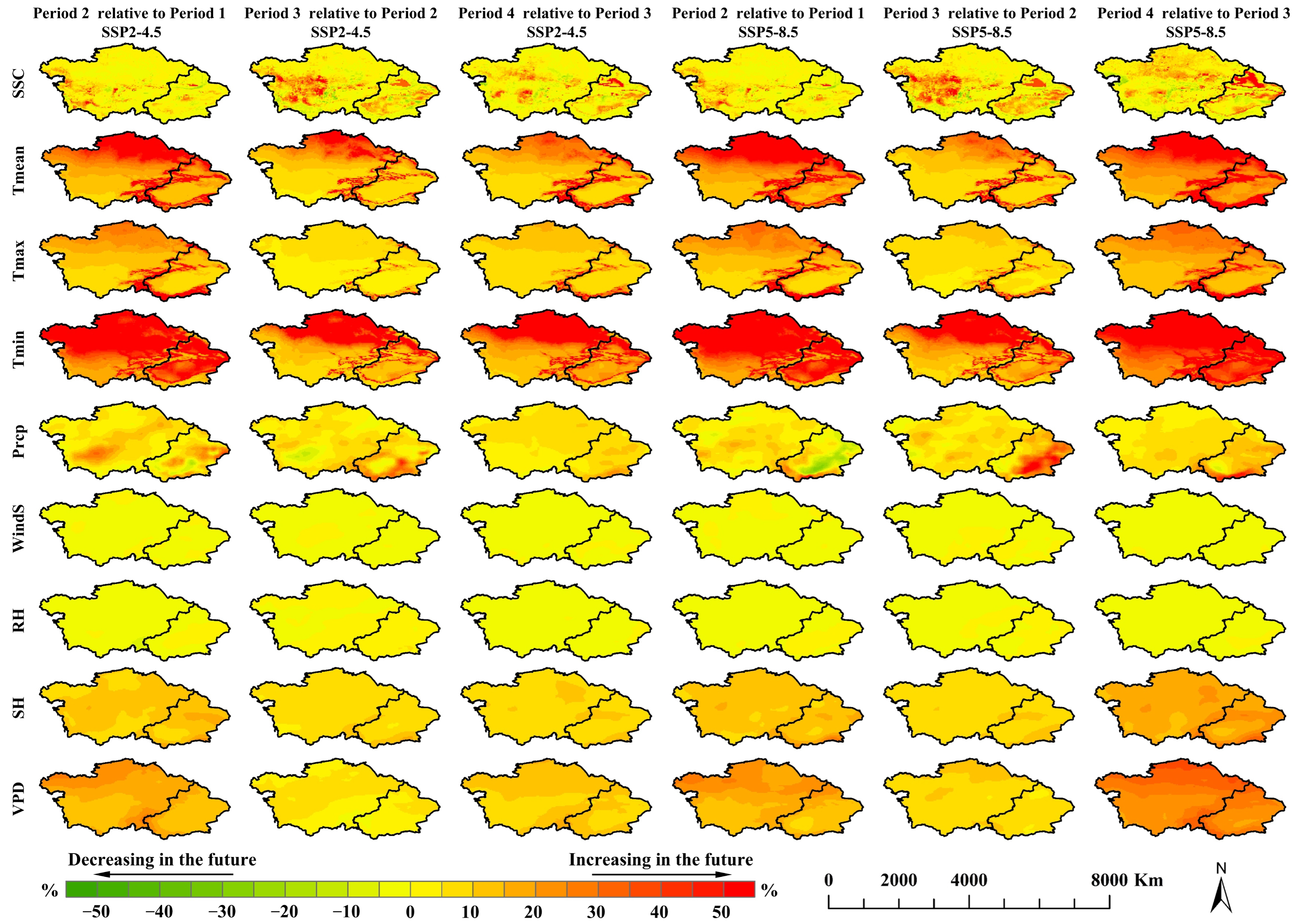
3.4.1. Spatial Variation in Multiple Periods Under Different Scenarios

The relative spatial variation of factors is expressed based on the difference of mean value between two periods. As can be seen from Figure 6, the great variation in climate factors is temperature (including Tmean, Tmax, and Tmin), which shows a significant increasing trend in all periods, especially Tmin. The regions with large temperature changes are mainly distributed in Kazakhstan in northern Central Asia, the Altai Mountains, Tianshan Mountains, and Kunlun Mountains. This is followed by Prcp, SH, and VPS, whose relative rate of change is mainly distributed between 10% and 30%. WindS and RH change the least; their relative rate of change is almost less than 5%, and shows a large range of decreasing trends. In both SSP2-4.5 and SSP5-8.5 scenarios, SSC shows an increasing trend in the study area. Regions with severe SSC variation in Central Asia are mainly distributed around the Caspian Sea, Aral Sea, and Lake Balkashgar. Higher temperatures make these water bodies gradually shrink, so that the salt content in the water increases [68]. As the main irrigation water source in Central Asia, they will further increase the soil salinity of the surrounding cropland [12]. In Xinjiang, the areas with large SSC changes are mainly located in the Zhungeer Basin and the Tarim Basin. This may be due to the overall temperature increase in the study area and the increased precipitation in the mountainous area. The salt in the alpine soil flows into the low-elevation basin with precipitation, making the SSC in the basin increase [5,68]. Additionally, the soil salinity at the junction of mountains and basins is more severe.

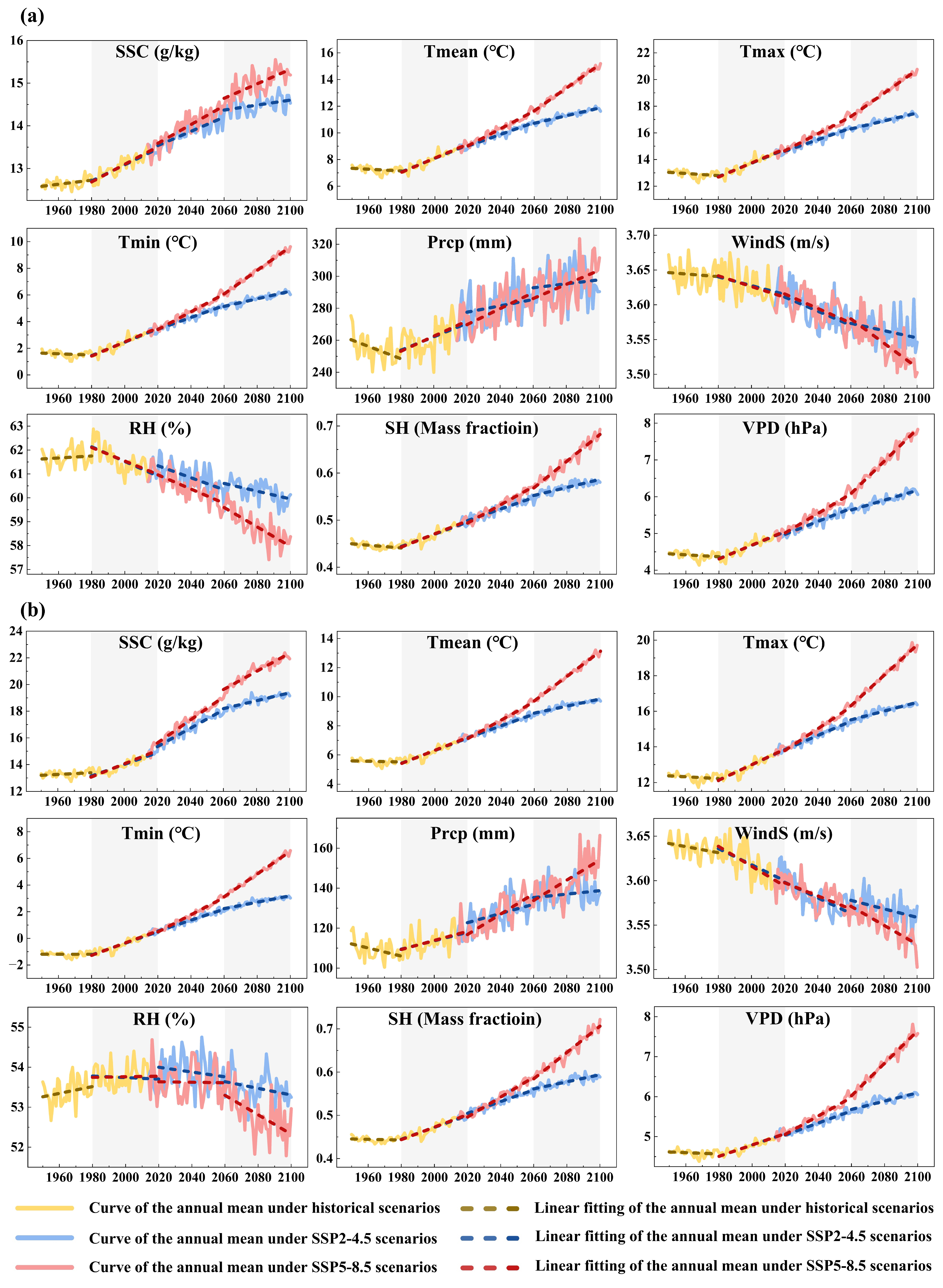
3.4.2. Long-Term Variation of the Study Area Under Different Scenarios

In this paper, temporal variations of factors are described by the annual mean value of the region. It is evident that from Period 2 to Period 4, temperature, Prcp, VPD, and SH exhibit an increasing trend in both study areas, while WindS and RH display a decreasing trend (Figure 7). This is opposite to their performance at Period 1. According to the range of SSC values, soil salinization in Xinjiang is more severe than in Central Asia. Comparing the two regions, Central Asia has higher temperatures, Prcp, and RH than Xinjiang. Therefore, these five associated features can be considered as the main climate factors causing the differences in SSC between the two regions. From 1950 to 2100, the mean SSC (g/kg) in Central Asia varies by +15.68% and +20.94% under the SSP2-4.5 and SSP5-8.5 scenarios, respectively (Figure 7a). At the same time, the eight climate factors (ordered by Tmean (℃), Tmax (℃), Tmin (℃), Prcp (mm), WindS (m/s), RH (%), SH (Mass fraction), and VPD (hPa)) vary by +53.50%, +30.45%, +209.23%, +5.47%, −3.27%, −3.06%, +26.09%, and +35.27% under the SSP2-4.5 scenario, while they vary by +97.36%, +54.55%, +386.15%, +15.13%, −3.81%, −5.88%, +56.52%, and +65.85% under the SSP5-8.5 scenario. In Xinjiang, the mean SSC from 1950 to 2100 varies by +43.88% and +64.76% under the SSP2-4.5 and SSP5-8.5 scenarios, respectively (Figure 7b). At the same time, the eight climate factors vary by +67.82%, +30.86%, +418.95%, +15.94%, −1.92%, −0.71%, +28.26%, and +30.70% under the SSP2-4.5 scenario, while they vary by +127.51%, +57.55%, +792.63%, +35.08%, −3.85%, −1.25%, +56.52%, and +63.71% under the SSP5-8.5 scenario. These climate change phenomena indicate that Central Asia and Xinjiang gradually dried out from 1950 to 2100 [69,70]. In general, under the influence of long-term climate warming, the soil salinization in drylands is continuously severe [1,53]. Additionally, the soil salinity in Xinjiang changes more significantly than that in Central Asia.

4. Discussion

4.1. Importance of Long-Term Climate Change on Salt-Affected Soils at Regional Scale

The spatial distribution (Figure 6) and temporal variation (Figure 7) of soil salinization under long-term climate change in Central Asia and Xinjiang were obtained based on an automated modeling framework. Our results revealed an increasing trend in soil salinization in Central Asia and Xinjiang under two scenarios. As the climate warms, the surface water evaporation intensifies, making the SH and VPD gradually increase [69], while the RH gradually decreases. At the same time, the decrease in WindS makes it difficult for the moisture of water bodies to be transmitted to other areas [70]. Since climate change under the SSP5-8.5 scenario is more extreme, its spatial variation of SSC is more pronounced than in the SSP2-4.5 scenarios [53]. To reveal the response of soil salinization to climate factors at the regional scale, this study quantitatively assessed the importance of temporal variations in individual climate factors on regional salt-affected soils from 1950 to 2100 (Figure 8). The contribution patterns of climate factors to SSC were similar in Central Asia and Xinjiang. Temperature, VPD, and SH were more important to SSC at a regional scale. High temperatures exacerbate soil water evaporation, leading to the accumulation of salts on the surface and accelerating soil salinization [31,71]. Rising VPD means that the amount of water vapor lost to the atmosphere through plant transpiration and soil evaporation increases, which will raise the risk of vegetation being subjected to drought stress [72,73]. Studies have shown that soil salinity is negatively correlated with vegetation coverage [6]. SH is the indicator of atmospheric dryness. The drought climate characteristic is the main cause of soil salinization [51]. The proportion of the importance of the variables to the soil salinity changes in different scenarios varied in the two study areas. Compared with the SSP2-4.5 scenario, temperature is more sensitive to SSC under the SSP5-8.5 scenario in Central Asia, while SH and VPD exhibit a greater contribution under the SSP5-8.5 scenario in Xinjiang. Moreover, Prep and RH are relatively important in Central Asia. Changes to Prcp and RH have the potential to further aggravate water scarcity [50]. Due to limited freshwater supplies, food production in drylands often depends on irrigation with high-salinity water, including treated wastewater and saline groundwater [48,74]. Climate change can lead to significant alterations in the frequency, magnitude, and spatial extent of soil moisture movement [51]. Therefore, research on the dynamic changes of soil salinization needs to focus more on the mechanisms by which terrestrial water cycle processes influence SSC.

4.2. The Prospects and Limitations of This Automated Soil Salinity Study

4.2.1. Uncertainty of the Data-Driven Model

Machine learning has shown robust performance and high accuracy in solving complex soil salinization problems. In our study, ET and XGBoost were identified as the better-performing algorithms. However, the differences in algorithm performance only reflect their adaptability in specific scenarios [35,36]. Each algorithm has its own advantages [23,30,31], making it essential to implement an automated modeling process that can automatically match the optimal algorithm and hyperparameter combination based on the unique characteristics of the data. This study employs the RMSE as the objective function to search for the optimal model, a metric that is widely applied in regression tasks for soil salinity modeling [27,31,32]. There are several metrics that take into account both model complexity and goodness of fit. For example, the Akaike Information Criterion (AIC), the Bayesian Information Criterion (BIC), and the corrected AIC (AICc), which are based on the maximum likelihood method, focus on the impact of the number of hyperparameters or sample size on the model outcomes [75,76]. Later studies may consider integrating different evaluation parameters to conduct unbiased assessments. Moreover, it should be noted that the training data will directly affect the prediction results of the machine learning model [8,35]. For large-scale studies (such as global research), it is more challenging for locations and time nodes with a small number of sample data. Machine learning models have data-driven properties, so they can predict results as long as there is a data input [27]. As a mathematical model, the machine learning model ignores the mechanistic process of soil salinization formation. Most mechanistic models require idealized assumptions and complex parameters, which limit their application at different scales [25,26]. At present, the combination of a machine learning model and a mechanistic model to construct a hybrid model has become a research hotspot in many fields [23]. Remote sensing is limited to capturing surface information [20]; thus, integrating the solute transport process from mechanistic models into machine learning frameworks could enable a more comprehensive exploration of the vertical distribution of salt in deep soils.

4.2.2. Uncertainty of the Feature Selection Process

One of the objectives of this study was to identify features that are significant for soil salinization. Generally, feature selection methods can be categorized into filter methods, wrapper methods, and embedded methods [77,78,79]. This paper employs the embedded feature selection method, which integrates the feature selection process with the learning process, thereby selecting features concurrently with model training [77]. For instance, Elastic Net combines the L1 LASSO penalty and the L2 penalty of Ridge regression [80,81]. Insignificant feature coefficients are reduced to zero through L1 regularization, while feature coefficients are penalized via L2 regularization to mitigate overfitting and collinearity issues [80,81]. These steps are primarily achieved by leveraging the hyperparameters of Elastic Net, specifically the regularization strength (alpha) and the weight ratio of the L1 and L2 regularization terms (L1_ratio). Other notable examples of embedded feature selection models are tree-based models [78,79], such as DT, RF, XGBoost, and CatBoost. These algorithms measure feature importance primarily through metrics such as gain, entropy, information gain, and information gain ratio [79]. Soil salinization is a major environmental risk caused by natural or human activities that is especially pronounced in drylands [6,7,8,9,10,11,12]. We have selected as many related environmental factors as possible, such as climate change, soil moisture, livestock, etc., but some factors are still excluded. One of the components of the SCORPAN framework is the parent material (weathered rock or deposit from which the soil is formed) [28,29,37], which could be incorporated to enhance our model in future studies. Water–salt movement is an important process in the formation of soil salinization, so the variation in SSC has a strong correlation with the water cycle [22,24]. There are studies that have shown that, as the carrier of soil salt, groundwater and irrigation water are closely related to soil water and salt transport [9,25,68], but access to these data at the regional scale is limited and difficult. Additionally, salt-affected soils are crucially affected by irrigation systems (drip, sprinkler, and surface irrigation) and fertilizer application [47,48].

4.2.3. Scale Effects of Soil Salinization

Soil salinization is susceptible to environmental factors and exhibits significant spatiotemporal heterogeneity [82]. The interaction effects exhibit remarkable characteristics at different scales [82,83]. Multi-source remote sensing imagery possesses multi-resolution (multi-scale) characteristics, and the richness of ground object information varies significantly at different scales. With historical and future climate changes, we use long-term climate data provided by CMIP6 to predict spatiotemporal variation of SSC from 1950 to 2100. The spatial resolution of CMIP6 is relatively coarse (0.25°) [1,55]. Although the bilinear interpolation method was employed to standardize the image resolution, this statistical resampling approach cannot fully capture the complexity of the climate system. Additionally, the effectiveness of the interpolation results has not been assessed. This problem may be resolved by integrating downscaling methods to produce long-term climate data with a higher spatial resolution in the future. Furthermore, soil salinization exhibits scale dependence, where certain patterns are only discernible at specific scales [83,84]. In our results, the importance of climate factors for SSC differs at the pixel (Figure 4) and regional scales (Figure 8). It has been proved that the influence of natural factors was mainly concentrated at large-scale salt-affected soils, while the impact of human activities was more obvious on the small scale [49,84]. Therefore, determining the optimal scale for soil salinization research in different study areas deserves further attention. Moreover, this paper predicts the long-term spatial distribution of regional soil salinization based on multi-year soil sampling data. Soil salinization exhibits distinct seasonal variation patterns, which varied with vegetation type and water application [38,51]. Therefore, we will next focus on the seasonal variations of soil salinity in the horizontal and vertical directions by comparing datasets collected in different seasons.

5. Conclusions

In this study, an automated machine learning framework was developed utilizing years of field-collected soil samples, which are capable of predicting SSC without the need for manual intervention. This framework also identified key driving factors, encompassing natural causes and human actions, that significantly influence soil salinization. Our results indicate that, at the pixel scale, precipitation and temperature are significant factors on SSC in Central Asia and Xinjiang, respectively. Meanwhile, meteorological factors have the greatest influence on the spatial and temporal variations of soil salinization in the two studied areas. Soil salinization intensifies with long-term climate warming. From 1950 to 2100, temperature, VPD, and SH exhibit significance for SSC at the regional scale. In conclusion, our study provides an automated framework for interaction analysis of driving factors on salt-affected soils in drylands, which has shown a robust and adaptive performance in different study areas.

References

1. Hassani, A.; Azapagic, A.; Shokri, N. Global predictions of primary soil salinization under changing climate in the 21st century. Nat. Commun. 2021, 12, 6663. [Google Scholar] [CrossRef]
2. Wang, J.Z.; Ding, J.L.; Yu, D.L.; Ma, X.K.; Zhang, Z.P.; Ge, X.Y.; Teng, D.X.; Li, X.H.; Liang, J.; Lizag, A.; et al. Capability of Sentinel-2 MSI data for monitoring and mapping of soil salinity in dry and wet seasons in the Ebinur Lake region, Xinjiang, China. Geoderma 2019, 353, 172–187. [Google Scholar] [CrossRef]
3. Zhao, W.J.; Ma, H.; Zhou, C.; Zhou, C.Q.; Li, Z.L. Soil Salinity Inversion Model Based on BPNN Optimization Algorithm for UAV Multispectral Remote Sensing. IEEE J. Sel. Top. Appl. Earth Obs. Remote Sens. 2023, 16, 6038–6047. [Google Scholar] [CrossRef]
4. Wang, N.; Peng, J.; Xue, J.; Zhang, X.L.; Huang, J.Y.; Biswas, A.; He, Y.; Shi, Z. A framework for determining the total salt content of soil profiles using time-series Sentinel-2 images and a random forest-temporal convolution network. Geoderma 2022, 409, 115656. [Google Scholar] [CrossRef]
5. Castro, F.C.; Araújo, J.F.; dos Santos, A.M. Susceptibility to soil salinization in the quilombola community of Cupira—Santa Maria da Boa Vista—Pernambuco—Brazil. Catena 2019, 179, 175–183. [Google Scholar] [CrossRef]
6. Mukhopadhyay, R.; Sarkar, B.; Jat, H.S.; Sharma, P.C.; Bolan, N.S. Soil salinity under climate change: Challenges for sustainable agriculture and food security. J. Environ. Manag. 2021, 280, 111736. [Google Scholar] [CrossRef]
7. FAO. Global Status of Salt-Affected Soils; Food and Agriculture Organization of the United Nations: Rome, Italy, 2024; Available online: https://openknowledge.fao.org/handle/20.500.14283/cd3044en (accessed on 15 December 2024).
8. Wang, Z.; Zhang, X.L.; Zhang, F.; Chan, N.W.; Kung, H.T.; Liu, S.H.; Deng, L.F. Estimation of soil salt content using machine learning techniques based on remote-sensing fractional derivatives, a case study in the Ebinur Lake Wetland National Nature Reserve, Northwest China. Ecol. Indic. 2020, 119, 106869. [Google Scholar] [CrossRef]
9. Zhang, Y.T.; Hou, K.; Qian, H.; Gao, Y.Y.; Fang, Y.; Xiao, S.; Tang, S.Q.; Zhang, Q.Y.; Qu, W.A.; Ren, W.H. Characterization of soil salinization and its driving factors in a typical irrigation area of Northwest China. Sci. Total Environ. 2022, 837, 155808. [Google Scholar] [CrossRef]
10. Gorji, T.; Sertel, E.; Tanik, A. Monitoring soil salinity via remote sensing technology under data scarce conditions: A case study from Turkey. Ecol. Indic. 2017, 74, 384–391. [Google Scholar] [CrossRef]
11. Li, Y.S.; Chang, C.Y.; Wang, Z.R.; Zhao, G.X. Upscaling remote sensing inversion and dynamic monitoring of soil salinization in the Yellow River Delta, China. Ecol. Indic. 2023, 148, 110087. [Google Scholar] [CrossRef]
12. Masoud, A.A.; Koike, K.; Atwia, M.G.; El-Horiny, M.M.; Gemail, K.S. Mapping soil salinity using spectral mixture analysis of landsat 8 OLI images to identify factors influencing salinization in an arid region. Int. J. Appl. Earth Obs. Geoinf. 2019, 83, 101944. [Google Scholar] [CrossRef]
13. Zhang, X.D.; Shu, C.J.; Wu, Y.J.; Ye, P.; Du, D.W. Advances of coupled water-heat-salt theory and test techniques for soils in cold and arid regions: A review. Geoderma 2023, 432, 116378. [Google Scholar] [CrossRef]
14. Li, W.H.; Kang, S.Z.; Du, T.S.; Ding, R.S.; Zou, M.Z. Optimal groundwater depth and irrigation amount can mitigate secondary salinization in water-saving irrigated areas in arid regions. Agric. Water Manag. 2024, 302, 109007. [Google Scholar] [CrossRef]
15. Salcedo, F.P.; Cutillas, P.P.; Cabañero, J.J.A.; Vivaldi, A.G. Use of remote sensing to evaluate the effects of environmental factors on soil salinity in a semi-arid area. Sci. Total Environ. 2022, 815, 152524. [Google Scholar] [CrossRef]
16. Tang, H.; Du, L.; Xia, C.C.; Luo, J. Bridging gaps and seeding futures: A synthesis of soil salinization and the role of plant-soil interactions under climate change. Iscience 2024, 27, 110804. [Google Scholar] [CrossRef]
17. Bai, J.D.; Wang, N.; Hu, B.F.; Feng, C.H.; Wang, Y.Z.; Peng, J.; Shi, Z. Integrating multisource information to delineate oasis farmland salinity management zones in southern Xinjiang, China. Agric. Water Manag. 2023, 289, 108559. [Google Scholar] [CrossRef]
18. Ma, S.L.; He, B.Z.; Xie, B.Q.; Ge, X.Y.; Han, L.J. Investigation of the spatial and temporal variation of soil salinity using Google Earth Engine: A case study at Werigan-Kuqa Oasis, West China. Sci. Rep. 2023, 13, 2754. [Google Scholar] [CrossRef] [PubMed]
19. Du, D.Y.; He, B.Z.; Luo, X.F.; Ma, S.L.; Song, Y.N.; Yang, W. Spatio-Temporal Variation Analysis of Soil Salinization in the Ougan-Kuqa River Oasis of China. Sustainability 2024, 16, 2706. [Google Scholar] [CrossRef]
20. Wang, N.; Xue, J.; Peng, J.; Biswas, A.; He, Y.; Shi, Z. Integrating Remote Sensing and Landscape Characteristics to Estimate Soil Salinity Using Machine Learning Methods: A Case Study from Southern Xinjiang, China. Remote Sens. 2020, 12, 4118. [Google Scholar] [CrossRef]
21. Xu, H.T.; Chen, C.B.; Zheng, H.W.; Luo, G.P.; Yang, L.; Wang, W.S.; Wu, S.X.; Ding, J.L. AGA-SVR-based selection of feature subsets and optimization of parameter in regional soil salinization monitoring. Int. J. Remote Sens. 2020, 41, 4470–4495. [Google Scholar] [CrossRef]
22. Devkota, K.P.; Devkota, M.; Rezaei, M.; Oosterbaan, R. Managing salinity for sustainable agricultural production in salt-affected soils of irrigated drylands. Agric. Syst. 2022, 198, 103390. [Google Scholar] [CrossRef]
23. Dong, L.M.; Lei, G.Q.; Huang, J.S.; Zeng, W.Z. Improving crop modeling in saline soils by predicting root length density dynamics with machine learning algorithms. Agric. Water Manag. 2023, 287, 108425. [Google Scholar] [CrossRef]
24. Bailey, R.T.; Tavakoli-Kivi, S.; Wei, X.L. A salinity module for SWAT to simulate salt ion fate and transport at the watershed scale. HESS 2019, 23, 3155–3174. [Google Scholar] [CrossRef]
25. Ren, D.Y.; Wei, B.Y.; Xu, X.; Engel, B.; Li, G.Y.; Huang, Q.Z.; Xiong, Y.W.; Huang, G.H. Analyzing spatiotemporal characteristics of soil salinity in arid irrigated agro-ecosystems using integrated approaches. Geoderma 2019, 356, 113935. [Google Scholar] [CrossRef]
26. Karimzadeh, S.; Hartman, S.; Chiarelli, D.D.; Rulli, M.C.; D’Odorico, P. The tradeoff between water savings and salinization prevention in dryland irrigation. AdWR 2024, 183, 104604. [Google Scholar] [CrossRef]
27. Wang, L.Y.; Hu, P.; Zheng, H.W.; Liu, Y.; Cao, X.W.; Hellwich, O.; Liu, T.; Luo, G.P.; Bao, A.M.; Chen, X. Integrative modeling of heterogeneous soil salinity using sparse ground samples and remote sensing images. Geoderma 2023, 430, 116321. [Google Scholar] [CrossRef]
28. Lozbenev, N.; Yurova, A.; Smirnova, M.; Kozlov, D. Incorporating process-based modeling into digital soil mapping: A case study in the virgin steppe of the Central Russian Upland. Geoderma 2021, 383, 114733. [Google Scholar] [CrossRef]
29. Belkadi, W.H.; Drias, Y.; Drias, H.; Dali, M.; Hamdous, S.; Kamel, N.; Aksa, D. A SCORPAN-based data warehouse for digital soil mapping and association rule mining in support of sustainable agriculture and climate change analysis in the Maghreb region. Expert Syst. 2024, 41, e13464. [Google Scholar] [CrossRef]
30. Brungard, C.W.; Boettinger, J.L.; Duniway, M.C.; Wills, S.A.; Edwards, T.C. Machine learning for predicting soil classes in three semi-arid landscapes. Geoderma 2015, 239, 68–83. [Google Scholar] [CrossRef]
31. Zhang, M.L.; Fan, X.L.; Gao, P.; Guo, L.; Huang, X.R.; Gao, X.W.; Pang, J.P.; Tan, F. Monitoring Soil Salinity in Arid Areas of Northern Xinjiang Using Multi-Source Satellite Data: A Trusted Deep Learning Framework. Land 2025, 14, 110. [Google Scholar] [CrossRef]
32. Liu, Y.N.; Han, X.D.; Zhu, Y.; Li, H.; Qian, Y.Z.; Wang, K.; Ye, M. Spatial mapping and driving factor Identification for salt-affected soils at continental scale using Machine learning methods. J. Hydrol. 2024, 639, 131589. [Google Scholar] [CrossRef]
33. Wang, J.Z.; Ding, J.L.; Yu, D.L.; Teng, D.X.; He, B.; Chen, X.Y.; Ge, X.Y.; Zhang, Z.P.; Wang, Y.; Yang, X.D.; et al. Machine learning-based detection of soil salinity in an arid desert region, Northwest China: A comparison between Landsat-8 OLI and Sentinel-2 MSI. Sci. Total Environ. 2020, 707, 136092. [Google Scholar] [CrossRef]
34. Xu, S.X.; Zhao, Y.C.; Wang, Y.Y. Optimizing machine learning models for predicting soil pH and total P in intact soil profiles with visible and near-infrared reflectance (VNIR) spectroscopy. Comput. Electron. Agric. 2024, 218, 108643. [Google Scholar] [CrossRef]
35. Han, Y.; Ge, H.T.; Xu, Y.P.; Zhuang, L.J.; Wang, F.Y.; Gu, Q.Y.; Li, X.J. Estimating Soil Salinity Using Multiple Spectral Indexes and Machine Learning Algorithm in Songnen Plain, China. IEEE J. Sel. Top. Appl. Earth Obs. Remote Sens. 2023, 16, 7041–7050. [Google Scholar] [CrossRef]
36. Chen, B.L.; Zheng, H.W.; Luo, G.P.; Chen, C.B.; Bao, A.M.; Liu, T.; Chen, X. Adaptive estimation of multi-regional soil salinization using extreme gradient boosting with Bayesian TPE optimization. Int. J. Remote Sens. 2022, 43, 778–811. [Google Scholar] [CrossRef]
37. McBratney, A.B.; Santos, M.L.M.; Minasny, B. On digital soil mapping. Geoderma 2003, 117, 3–52. [Google Scholar] [CrossRef]
38. Perri, S.; Molini, A.; Hedin, L.O.; Porporato, A. Contrasting effects of aridity and seasonality on global salinization. Nat. Geosci. 2022, 15, 375–381. [Google Scholar] [CrossRef]
39. Zhang, Y.; Wu, H.Q.; Kang, Y.L.; Fan, Y.M.; Wang, S.S.; Liu, Z.; He, F.F. Mapping the Soil Salinity Distribution and Analyzing Its Spatial and Temporal Changes in Bachu County, Xinjiang, Based on Google Earth Engine and Machine Learning. Agriculture 2024, 14, 630. [Google Scholar] [CrossRef]
40. Dwivedi, R.; Dave, D.; Naik, H.; Singhal, S.; Omer, R.; Patel, P.; Qian, B.; Wen, Z.Y.; Shah, T.; Morgan, G.; et al. Explainable AI (XAI): Core Ideas, Techniques, and Solutions. Acm Comput. Surv. 2023, 55, 1–33. [Google Scholar] [CrossRef]
41. Li, Z.Q. Extracting spatial effects from machine learning model using local interpretation method: An example of SHAP and XGBoost. Comput. Environ. Urban Syst. 2022, 96, 101845. [Google Scholar] [CrossRef]
42. Lundberg, S.M.; Lee, S.I. A Unified Approach to Interpreting Model Predictions. In Proceedings of the 31st Annual Conference on Neural Information Processing Systems (NIPS), Long Beach, CA, USA, 4–9 December 2017. [Google Scholar]
43. Ribeiro, M.T.; Singh, S.; Guestrin, C.; Assoc Comp, M. “Why Should I Trust You?” Explaining the Predictions of Any Classifier. In Proceedings of the 22nd ACM SIGKDD International Conference on Knowledge Discovery and Data Mining (KDD), San Francisco, CA, USA, 13–17 August 2016; pp. 1135–1144. [Google Scholar]
44. Friedman, J.H. Greedy function approximation: A gradient boosting machine. Ann. Stat. 2001, 29, 1189–1232. [Google Scholar] [CrossRef]
45. Measho, S.; Li, F.D.; Pellikka, P.; Tian, C.; Hirwa, H.; Xu, N.; Qiao, Y.F.; Khasanov, S.; Kulmatov, R.; Chen, G. Soil Salinity Variations and Associated Implications for Agriculture and Land Resources Development Using Remote Sensing Datasets in Central Asia. Remote Sens. 2022, 14, 2501. [Google Scholar] [CrossRef]
46. Suska-Malawska, M.; Vyrakhamanova, A.; Ibraeva, M.; Poshanov, M.; Sulwinski, M.; Toderich, K.; Metrak, M. Spatial and In-Depth Distribution of Soil Salinity and Heavy Metals (Pb, Zn, Cd, Ni, Cu) in Arable Irrigated Soils in Southern Kazakhstan. Agronomy 2022, 12, 1207. [Google Scholar] [CrossRef]
47. Ayana, D.; Yermekkul, Z.; Issakov, Y.; Mirobit, M.; Ainura, A.; Yerbolat, K.; Ainur, K.; Kairat, Z.; Zhu, K.; Dávid, L.D. The possibility of using groundwater and collector-drainage water to increase water availability in the Maktaaral district of the Turkestan region of Kazakhstan. Agric. Water Manag. 2024, 301, 108934. [Google Scholar] [CrossRef]
48. Liu, C.; Liu, H.; Yu, Y.; Zhao, W.Z.; Zhang, Z.; Guo, L.; Yetemen, O. Mapping groundwater-dependent ecosystems in arid Central Asia: Implications for controlling regional land degradation. Sci. Total Environ. 2021, 797, 149027. [Google Scholar] [CrossRef] [PubMed]
49. Zhang, W.T.; Wu, H.Q.; Gu, H.B.; Feng, G.L.; Wang, Z.; Sheng, J.D. Variability of Soil Salinity at Multiple Spatio-Temporal Scales and the Related Driving Factors in the Oasis Areas of Xinjiang, China. Pedosphere 2014, 24, 753–762. [Google Scholar] [CrossRef]
50. Han, L.J.; Ding, J.L.; Zhang, J.Y.; Chen, P.P.; Wang, J.Z.; Wang, Y.H.; Wang, J.J.; Ge, X.Y.; Zhang, Z.P. Precipitation events determine the spatiotemporal distribution of playa surface salinity in arid regions: Evidence from satellite data fused via the enhanced spatial and temporal adaptive reflectance fusion model. Catena 2021, 206, 105546. [Google Scholar] [CrossRef]
51. Wang, J.; Xue, L.Q.; Liu, H.L.; Cao, B.; Bai, Y.A.; Xiang, C.G.; Li, X.H. Patterns of salt transport and factors affecting typical shrub in desert-oases transition areas. Environ. Res. 2023, 236, 116804. [Google Scholar] [CrossRef]
52. Khasanov, S.; Kulmatov, R.; Li, F.D.; van Amstel, A.; Bartholomeus, H.; Aslanov, I.; Sultonov, K.; Kholov, N.; Liu, H.G.; Chen, G. Impact assessment of soil salinity on crop production in Uzbekistan and its global significance. Agric. Ecosyst. Environ. 2023, 342, 108262. [Google Scholar] [CrossRef]
53. Dong, X.; Ding, J.L.; Ge, X.Y. Future changes in soil salinization across Central Asia under CMIP6 forcing scenarios. Land Degrad. Dev. 2024, 35, 3981–3998. [Google Scholar] [CrossRef]
54. Thrasher, B.; Wang, W.L.; Michaelis, A.; Melton, F.; Lee, T.; Nemani, R. NASA Global Daily Downscaled Projections, CMIP6. Sci. Data 2022, 9, 262. [Google Scholar] [CrossRef]
55. Wu, F.; Jiao, D.L.; Yang, X.L.; Cui, Z.Y.; Zhang, H.S.; Wang, Y.H. Evaluation of NEX-GDDP-CMIP6 in simulation performance and drought capture utility over China—Based on DISO. Hydrol. Res. 2023, 54, 703–721. [Google Scholar] [CrossRef]
56. Chen, G.Z.; Li, X.; Liu, X.P. Global land projection based on plant functional types with a 1-km resolution under socio-climatic scenarios. Sci. Data 2022, 9, 125. [Google Scholar] [CrossRef]
57. Kolluru, V.; John, R.; Saraf, S.; Chen, J.Q.; Hankerson, B.; Robinson, S.; Kussainova, M.; Jain, K. Gridded livestock density database and spatial trends for Kazakhstan. Sci. Data 2023, 10, 839. [Google Scholar] [CrossRef] [PubMed]
58. Fick, S.E.; Belnap, J.; Duniway, M.C. Grazing-Induced Changes to Biological Soil Crust Cover Mediate Hillslope Erosion in Long-Term Exclosure Experiment. Rangel. Ecol. Manag. 2020, 73, 61–72. [Google Scholar] [CrossRef]
59. Macheroum, A.; Sayada, N.; Chenchouni, H. Restoration of soil quality and improvement of physicochemical properties through grazing exclusion in arid and semi-arid rangelands. Catena 2025, 249, 108646. [Google Scholar] [CrossRef]
60. Gilbert, M.; Nicolas, G.; Cinardi, G.; Van Boeckel, T.P.; Vanwambeke, S.O.; Wint, G.R.W.; Robinson, T.P. Global distribution data for cattle, buffaloes, horses, sheep, goats, pigs, chickens and ducks in 2010. Sci. Data 2018, 5, 180227. [Google Scholar] [CrossRef]
61. Shahriari, B.; Swersky, K.; Wang, Z.Y.; Adams, R.P.; de Freitas, N. Taking the Human Out of the Loop: A Review of Bayesian Optimization. Proc. IEEE 2016, 104, 148–175. [Google Scholar] [CrossRef]
62. Strumbelj, E.; Kononenko, I. Explaining prediction models and individual predictions with feature contributions. Knowl. Inf. Syst. 2014, 41, 647–665. [Google Scholar] [CrossRef]
63. Lundberg, S.M.; Erion, G.; Chen, H.; DeGrave, A.; Prutkin, J.M.; Nair, B.; Katz, R.; Himmelfarb, J.; Bansal, N.; Lee, S.I. From local explanations to global understanding with explainable AI for trees. Nat. Mach. Intell. 2020, 2, 56–67. [Google Scholar] [CrossRef]
64. Wang, S.Z.; Li, W.W.; Gu, Z.N. GeoGraphViz: Geographically constrained 3D force-directed graph for knowledge graph visualization. Trans. Gis 2023, 27, 931–948. [Google Scholar] [CrossRef]
65. Hua, J.; Wang, G.H.; Xu, Y.Q. Adopting Centrality Measure Models in Visualized Financial Datasets. In Proceedings of the 2nd the International Conference on Image and Video Processing, and Artificial Intelligence (IPVAI), Shanghai, China, 23–25 August 2019. [Google Scholar]
66. Jacomy, M.; Venturini, T.; Heymann, S.; Bastian, M. ForceAtlas2, a Continuous Graph Layout Algorithm for Handy Network Visualization Designed for the Gephi Software. PLoS ONE 2014, 9, e98679. [Google Scholar] [CrossRef] [PubMed]
67. Gouvêa, A.; da Silva, T.S.; Macau, E.E.N.; Quiles, M.G. Force-directed algorithms as a tool to support community detection. Eur. Phys. J. -Spec. Top. 2021, 230, 2745–2763. [Google Scholar] [CrossRef]
68. Liu, W.L.; Jiang, L.L.; Jiapaer, G.; Wu, G.M.; Li, Q.J.; Yang, J. Monitoring the salinization of agricultural land and assessing its drivers in the Altay region. Ecol. Indic. 2024, 167, 112678. [Google Scholar] [CrossRef]
69. Dai, A.G.; Zhao, T.B.; Chen, J. Climate Change and Drought: A Precipitation and Evaporation Perspective. Curr. Clim. Change Rep. 2018, 4, 301–312. [Google Scholar] [CrossRef]
70. Gimeno-Sotelo, L.; Sorí, R.; Nieto, R.; Vicente-Serrano, S.M.; Gimeno, L. Unravelling the origin of the atmospheric moisture deficit that leads to droughts. Nat. Water 2024, 2, 242–253. [Google Scholar] [CrossRef]
71. Khosravichenar, A.; Aalijahan, M.; Moaazeni, S.; Lupo, A.R.; Karimi, A.; Ulrich, M.; Parvian, N.; Sadeghi, A.; von Suchodoletz, H. Assessing a multi-method approach for dryland soil salinization with respect to climate change and global warming-The example of the Bajestan region (NE Iran). Ecol. Indic. 2023, 154, 110639. [Google Scholar] [CrossRef]
72. Zhong, Z.Q.; He, B.; Wang, Y.P.; Chen, H.W.; Chen, D.L.; Fu, Y.H.; Chen, Y.N.; Guo, L.L.; Deng, Y.; Huang, L.; et al. Disentangling the effects of vapor pressure deficit on northern terrestrial vegetation productivity. Sci. Adv. 2023, 9, eadf3166. [Google Scholar] [CrossRef]
73. Yuan, W.P.; Zheng, Y.; Piao, S.L.; Ciais, P.; Lombardozzi, D.; Wang, Y.P.; Ryu, Y.; Chen, G.X.; Dong, W.J.; Hu, Z.M.; et al. Increased atmospheric vapor pressure deficit reduces global vegetation growth. Sci. Adv. 2019, 5, eaax1396. [Google Scholar] [CrossRef]
74. Kramer, I.; Peleg, N.; Mau, Y. Climate change shifts risk of soil salinity and land degradation in water-scarce regions. Agric. Water Manag. 2025, 307, 109223. [Google Scholar] [CrossRef]
75. Bhadani, V.; Singh, A.; Kumar, V.; Gaurav, K. Nature-inspired optimal tuning of input membership functions of fuzzy inference system for groundwater level prediction. Environ. Model. Softw. 2024, 175, 105995. [Google Scholar] [CrossRef]
76. Singh, A.; Gaurav, K.; Rai, A.K.; Beg, Z. Machine Learning to Estimate Surface Roughness from Satellite Images. Remote Sens. 2021, 13, 3794. [Google Scholar] [CrossRef]
77. Jenul, A.; Schrunner, S.; Liland, K.H.; Indahl, U.G.; Futsaether, C.M.; Tomic, O. RENT-Repeated Elastic Net Technique for Feature Selection. IEEE Access 2021, 9, 152333–152346. [Google Scholar] [CrossRef]
78. Ferhatoglu, C.; Miller, B.A. Choosing Feature Selection Methods for Spatial Modeling of Soil Fertility Properties at the Field Scale. Agronomy 2022, 12, 1786. [Google Scholar] [CrossRef]
79. Guo, W.D.; Zhou, Z.Z. A comparative study of combining tree-based feature selection methods and classifiers in personal loan default prediction. J. Forecast. 2022, 41, 1248–1313. [Google Scholar] [CrossRef]
80. Zou, H.; Hastie, T. Regularization and variable selection via the elastic net. J. R. Stat. Soc. Ser. B-Stat. Methodol. 2005, 67, 301–320. [Google Scholar] [CrossRef]
81. Qaraad, M.; Amjad, S.; Manhrawy, I.I.M.; Fathi, H.; Hassan, B.A.; El Kafrawy, P. A Hybrid Feature Selection Optimization Model for High Dimension Data Classification. IEEE Access 2021, 9, 42884–42895. [Google Scholar] [CrossRef]
82. Chen, H.F.; Wu, J.W.; Xu, C. Monitoring Soil Salinity Classes through Remote Sensing-Based Ensemble Learning Concept: Considering Scale Effects. Remote Sens. 2024, 16, 642. [Google Scholar] [CrossRef]
83. Wei, Y.; Ding, J.L.; Yang, S.T.; Wang, F.; Wang, C. Soil salinity prediction based on scale-dependent relationships with environmental variables by discrete wavelet transform in the Tarim Basin. Catena 2021, 196, 104939. [Google Scholar] [CrossRef]
84. Zhu, C.M.; Ding, J.L.; Zhang, Z.P. Revealing the scale- and location-specific variation and control factors of soil salinity using bi-dimensional empirical modal decomposition. Land Degrad. Dev. 2022, 33, 3446–3460. [Google Scholar] [CrossRef]
Figure 1. Workflows. (a) Automated modeling for SSC. First, soil field samples and multivariate environmental factors were obtained for model training. Then, a method was built that could automatically search for the best combination of algorithm, hyperparameters, and features in the Bayesian optimization framework. Finally, the performance of the optimal model was evaluated using statistical metrics. (b) Nonlinear interactions analysis between SSC-related variables based on SHAP value and graph layout algorithm. (c) Exploration of the spatial and temporal variation of SSC with long-term climate change.
Remotesensing 17 00987 g001
Figure 2. The geographical location of the study area and sample points. (a) Represents the land-cover types in the study area, (b) is the location of the study area, (c) represents the distribution of sampling points and the ranges of Central Asia and Xinjiang, respectively, the basemap layer is from the ArcGIS online map, and (d,e) are the proportions of different SSCs in Central Asia and Xinjiang, respectively.
Remotesensing 17 00987 g002
Figure 3. Performance of the automated model in two study areas. (a,b) are the automatic search processes for the optimal model in Central Asia and Xinjiang, respectively. (c,e) are the accuracy evaluations of model predicted values versus observed values of SSC on the training and testing sets in Central Asia. (d,f) are the accuracy evaluation of model predicted values versus observed values of SSC on the training and testing sets in Xinjiang. The SD is abbreviated for the standard deviation.
Remotesensing 17 00987 g003
Figure 4. Importance interpretation of the input features based on the SHAP value. (a,b) are the top 15 important main features and their interaction effects in Central Asia and Xinjiang, respectively. (c,d) are the interaction-dependent graphs of the most important feature and its strongest interaction effect in the two study areas, respectively. The horizontal axis represents the observed value of the main feature and the vertical axis represents the SHAP value of the main feature. Each point represents a sample whose color characterizes the observed values of the interaction features. When SHAP > 0, the current corresponding feature has a positive effect on SSC, while when SHAP < 0, it indicates that the feature has a negative effect on SSC. The closer the SHAP value is to zero, the slighter the effect the feature has on SSC.
Remotesensing 17 00987 g004
Figure 5. Importance visualization of feature groups in the study areas. (a,b) are the layout graphs of the interaction relationships between the feature groups in Central Asia and Xinjiang, respectively. In the figure, the circle color indicates the feature group category, and the circle size indicates the importance of the feature group. Larger circles indicate greater contributions of the feature group to the SSC. Lines represent the interaction between groups, and the stronger the interaction, the thicker the lines. Groups with strong interaction were relatively close and those with weak interaction were relatively far away. (c,d) are the interaction graphs of feature groups and spatial and temporal indicators in Central Asia and Xinjiang, respectively. The horizontal axis represents the interaction between feature groups and longitude, and the vertical axis represent the interactions between feature groups and latitude. The circle size represents the interactions between feature groups and year.
Remotesensing 17 00987 g005
Figure 6. Spatial variation of soil salinity and eight climate factors in Central Asia and Xinjiang. The spatial relative changes are calculated based on the mean SSC for multiple periods using the formula (Future mean − Previous mean)/abs (Previous mean). The value of each pixel represents the percentage of relative changes and is presented by the color map. Positive values indicate an increase in SSC while the negative values are indicative of a decreasing trend.
Remotesensing 17 00987 g006
Figure 7. Long-term variation of soil salinity and eight climate factors in the study areas. (a,b) are regional mean changes from 1950 to 2100 in Central Asia and Xinjiang, respectively. The background color is used to divide the different periods. Solid lines represent the regional annual mean, dashed lines indicate the fitted variation trends. Different scenarios are presented by the colored lines.
Remotesensing 17 00987 g007
Figure 8. The importance of long-term climate factor variations to SSC at a regional scale. (a,b) illustrate the importance of temporal variations in individual climate factors on regional SSC under different scenarios in Central Asia and Xinjiang, respectively.
Remotesensing 17 00987 g008