SFIDM: Few-Shot Object Detection in Remote Sensing Images with Spatial-Frequency Interaction and Distribution Matching

Abstract

Few-shot object detection (FSOD) in remote sensing images (RSIs) faces challenges such as data scarcity, difficulty in detecting small objects, and underutilization of frequency-domain information. Existing methods often rely on spatial-domain features, neglecting the complementary insights from low- and high-frequency characteristics. Additionally, their performance in detecting small objects is hindered by inadequate feature extraction in cluttered backgrounds. To tackle these problems, we propose a novel detection framework of Spatial-Frequency Interaction and Distribution Matching (SFIDM), which significantly enhances FSOD performance in RSIs. SFIDM focuses on rapid adaptation to target datasets and efficient fine-tuning with limited data. First, to improve feature representation, we introduce the Spatial-Frequency Interaction (SFI) module, which leverages the complementarity between low-frequency and high-frequency information. By decomposing input images into their frequency components, the SFI module extracts features critical for classification and precise localization, enabling the framework to capture fine details essential for detecting small objects. Secondly, to resolve the limitations of traditional label assignment strategies when dealing with small bounding boxes, we construct the Distribution Matching (DM) module, which models bounding boxes as 2D Gaussian distributions. This allows for the accurate detection of subtle offsets and overlapping or non-overlapping small objects. Moreover, to leverage the learned base-class information for improved performance on novel class detection, we employ a feature reweighting module, which adaptively fuses features extracted from the backbone network to generate representations better suited for downstream detection tasks. We conducted extensive experiments on two benchmark FSOD datasets to demonstrate the effectiveness and performance improvements achieved by the proposed SFIDM framework.

1. Introduction

With the rapid advancement of satellite technology and the proliferation of large-scale image datasets [1,2,3], deep learning has become a cornerstone of remote sensing images (RSIs) interpretation, encompassing key tasks such as object detection [4,5,6], image classification [7,8,9], object recognition [10,11,12], image segmentation [13,14,15], and object tracking [16]. Among these, object detection (OD) serves as a foundational task in RSI analysis by providing instance-level information on object categories and locations, thereby supporting downstream applications such as environmental monitoring [17], urban planning [15], and disaster management [18].

Although recent advances in computer vision have greatly enhanced the analytical capabilities of RSIs, these achievements typically rely on large-scale annotated datasets [19]. In the remote sensing domain, the acquisition of such datasets is constrained by high costs and labor-intensive annotation processes, further limiting the construction of large, high-quality datasets [20,21]. Moreover, the increasing complexity of object detection models necessitates even larger datasets to fully exploit their potential. This disparity between the scarcity of RSI data and the demands of modern models poses a significant challenge, often leading to overfitting or performance degradation, especially for the OD task.

To tackle the unique challenges of remote sensing images (RSIs), including large intra-class variance, high inter-class similarity, scale variations, sparse annotations, and imbalanced data distributions, researchers have explored innovative approaches such as advanced feature extraction, optimized model architectures, and customized training strategies [22,23,24,25,26]. Despite these efforts, the complexity of RSIs and the scarcity of labeled data continue to hinder the progress of object detection (OD) in this domain, often resulting in feature misalignment, incomplete supervision, and attention biases. Few-Shot Object Detection (FSOD) has emerged as a promising solution, enabling models to generalize to new categories with minimal labeled examples by leveraging knowledge from data-rich base categories. Fine-tuning-based FSOD methods, in particular, have garnered significant attention [27,28,29] due to their streamlined architectures, minimized dependency on structured data, and enhanced practical applicability. These methods typically involve a two-stage process: training on base categories to learn generalizable feature representations, followed by fine-tuning novel categories with limited samples. However, directly applying FSOD techniques to remote sensing images (RSIs) presents additional challenges due to the significant variability in object sizes within the same scene. Objects in RSIs can range from small vehicles to large infrastructure, making it challenging for models to effectively capture features across such diverse scales. Notably, its extreme case—One-Shot Object Detection (OSOD)—further intensifies the challenge when only a single annotated instance is available, especially under RSIs’ inherent scale variations [30,31,32,33,34]. Integrating segmentation methods has also emerged as a direction in few-shot object detection [35,36,37,38,39,40]. Incorporating segmentation-assisted modules has shown promise in few-shot object detection by providing pixel-level foreground guidance to suppress background noise and enhance feature discriminability [41]. While segmentation-guided approaches could theoretically benefit both FSOD and OSOD scenarios, such methods often require additional segmentation annotations during training, which may introduce higher annotation costs or depend on weakly supervised approximations. Furthermore, existing FSOD and OSOD methods often fail to fully explore how frequency-domain information can be effectively integrated with spatial-domain features to improve detection performance. These challenges underscore the need for FSOD models specifically tailored to the unique scale variations and characteristics of RSIs, by incorporating domain-specific optimizations to enhance detection accuracy under data-limited conditions.

Building on these advancements, we propose a novel FSOD framework tailored for RSIs: Spatial-Frequency Interaction and Distribution Matching (SFIDM). Our approach integrates spatial and frequency-domain interactions with a robust distribution matching mechanism to address the unique challenges of FSOD in RSIs. We summarize our contributions as follows:

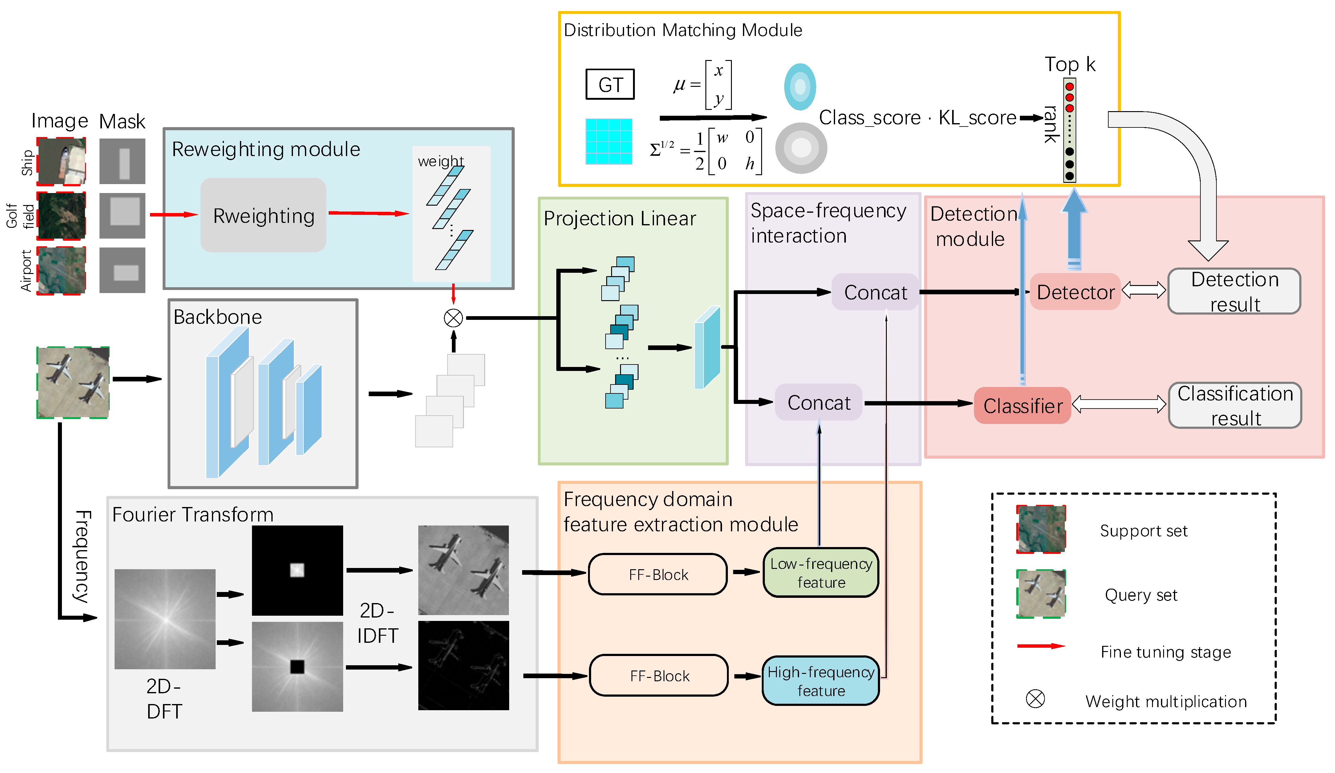
• To effectively leverage complementary frequency information, we introduce a mechanism that decomposes images into low-frequency and high-frequency components. Low-frequency components capture global structural patterns essential for classification, while high-frequency components focus on fine details crucial for precise localization. This design enhances the detection of small objects, particularly in complex backgrounds where traditional methods struggle.
• To improve label assignment, we employ a novel strategy of distribution matching that models bounding boxes as 2D Gaussian distributions. By utilizing Kullback–Leibler (KL) divergence [42] as a localization metric, this approach overcomes the limitations of traditional IoU-based heuristics, enabling accurate detection of subtle offsets and addressing the challenges posed by small or overlapping objects.
• We conducted experiments on publicly available datasets, DIOR and NWPU VHR-10, and performed comparative analyses between our proposed method and previous approaches. The results demonstrate the effectiveness and superiority of SFIDM. Furthermore, as a plug-and-play model, SFIDM can be seamlessly integrated with different backbone networks and detection frameworks, showcasing its versatility and adaptability.

The rest of this paper is organized as follows: Section 2 reviews the related work, focusing on few-shot object detection (FSOD) and its application in remote sensing scenarios. Section 3 presents our proposed method, detailing the overall framework and the design of its individual modules. Section 4 discusses the experimental results, highlighting the performance of our approach on the NWPU VHR-10 and DIOR datasets. Finally, Section 5 concludes the paper, summarizing the key contributions and findings.

2. Related Work

2.1. Few-Shot Object Detection in Natural Images

Few-Shot Object Detection (FSOD) aims to identify new or previously unseen object categories using only a small number of labeled examples. The primary challenge of FSOD lies in efficiently transferring existing knowledge to scenarios with limited data while maintaining strong generalization capabilities [29,43,44,45]. Currently, FSOD methods can be broadly categorized into three approaches: transfer learning-based methods, metric learning-based methods, and meta-learning-based methods.

2.1.1. Transfer Learning-Based Methods

Transfer learning-based methods fine-tune pre-trained models by transferring object detection models trained on base-class datasets to new classes [46,47,48,49]. The main advantage of this approach is that it eliminates the need to design complex training tasks, instead optimizing detection performance for new classes by leveraging transferred knowledge. Specifically, these methods utilize model parameters pre-trained on large-scale base-class datasets and transfer them to new-class data, enabling efficient object detection under few-shot conditions.

For example, LSTD [50], one of the early transfer learning methods, significantly improved detection accuracy by extracting rich features from base-class data and effectively transferring these features to target data. Meanwhile, TFA [51] simplified the training process by only fine-tuning the classification head and normalizing features using cosine similarity, successfully reducing intra-class variance and improving detection performance for new classes. Additionally, FSCE [52] introduced contrastive loss and optimized proposal encoding, further enhancing the discriminative ability of new-class features.

Although transfer learning methods show promising results, several challenges remain in few-shot object detection. Mostly, reducing category confusion between new and base classes and enhancing feature representations for new classes remain critical issues. Another significant challenge is how to ensure that base-class performance is maintained while improving new-class detection at the same time. Therefore, further research is urged to address issues such as category confusion and feature degradation, ensuring that improvements in new-class detection do not come at the expense of base-class performance.

2.1.2. Metric Learning-Based Methods

Metric learning-based methods aim to improve the ability to differentiate between various object categories by learning their similarities in the feature space, especially for the bounding-box classification tasks. These methods frame FSOD as a few-shot classification problem, employing a “comparison” strategy to address the issue of data scarcity. The core idea is to optimize feature representations through metric learning, providing effective classification cues for object detection. Optimization primarily focuses on three aspects: (1) enhancing the feature representation of support set images through class prototype representations [53,54], (2) improving inter-class separability and enhancing intra-class consistency through improved metric mechanisms [55,56], and (3) designing suitable loss functions to further optimize the model’s learning ability [32,57].

Note that object detection not only requires accurate classification but also precise localization of the target regions. Effective class comparison can only occur once the target’s location is determined. Therefore, metric learning-based detection must integrate target region capture mechanisms into the traditional metric learning framework. For instance, RepMet [55] models categories using Gaussian Mixture Models and optimizes the intra-class and inter-class distance differences through embedding loss, enhancing inter-class separability. Attention RPN [58] leverages support features to enhance region proposal generation, significantly reducing background noise interference. Although metric learning-based methods show significant advantages in feature representation and inter-class distinction, their performance still depends on the optimization of prototype design, metric mechanisms, and loss functions. Therefore, combining target localization techniques while retaining the advantages of metric learning remains an important direction in this line.

2.1.3. Meta-Learning-Based Methods

Meta-learning-based methods play a crucial role in FSOD. The core idea is to simulate a series of similar few-shot tasks, transferring prior knowledge learned from data-rich base classes to data-scarce new classes, thus addressing the issue of insufficient samples. In the meta-learning framework, the model is trained on tasks, typically by sampling both tasks and data to construct diverse new few-shot tasks. This strategy enables the model to quickly update parameters using a few support-set samples, achieving rapid generalization to new tasks, and, in some cases, even eliminating the need for further fine-tuning.

Meta-learning methods have shown significant success in FSOD. For example, MetaYOLO [43] improves the model’s adaptability to new classes by generating weight coefficients from support samples and dynamically adjusting the weight of query features. FsDetView [59] proposed a feature aggregation strategy that combines query and support features in a weighted manner, effectively enhancing detection performance for new classes. However, meta-learning methods are typically complex in design, requiring dynamic adjustments of multiple tasks during training. This may lead to convergence difficulties during iterations, limiting their practical application. Additionally, although these methods perform well in few-shot tasks, they are often constrained by low training efficiency and limited generalization ability.

Generally, few-shot object detection is a challenging research area, with ongoing advancements in methods and the combination of various strategies, such as integrating transfer learning with metric learning, to enhance the model’s ability to learn features for new classes. Other challenges include optimizing training efficiency, reducing category confusion, etc. Addressing these issues will be crucial to advancing the field of FSOD.

2.2. Few-Shot Object Detection in Remote Sensing Images

Remote sensing images (RSIs) have distinct characteristics, such as complex backgrounds, multi-directional objects, and significant scale variations, making the detection of small objects from these images a formidable challenge. Due to the significant differences between remote sensing and natural image acquisition principles, traditional object detection methods designed for natural images often struggle in remote sensing scenarios, especially when dealing with small objects and large-scale variations. Small objects are particularly prominent in remote sensing images and are often obscured by complex background information, making their detection difficult [60,61,62].

Focusing on data augmentation strategy, several studies have presented different solutions to small object detection in remote sensing images. For instance, Zhang et al. [63] introduced a directional feature enhancement method based on a dual-pipeline solution. This method enhances features by rotating single samples at multiple angles, which alleviates the issue of excessive intra-class variability. Cheng et al. [64] proposed a data augmentation strategy by randomly rotating each object instance five times at different angles, aiming to increase the diversity of the samples. However, while these methods somewhat mitigate the problem, the effectiveness of this augmentation approach is limited because the rotated samples still bear significant similarities to the original samples. In another line, several studies [65,66] integrated multi-scale feature fusion techniques to detect objects at various scales and enrich the diversity of feature representations. Attention mechanisms and learning strategies have been widely researched in few-shot settings. Huang et al. [67] proposed a few-shot fine-tuning network with a shared attention module (SAM) for object detection in remote sensing images. Xiao et al. [68] proposed a few-shot object detection method with a self-adaptive attention network (SAAN) tailored for remote sensing images. Liu et al. [69] proposed a novel few-shot object detection method that addresses inconsistent labeling by introducing a coarse-to-fine regression method (Gradual RPN) to enhance region proposal network (RPN) recall. Li et al. [70] proposed MM-RCNN, a meta-memory-based few-shot object detection approach that uses a memory module to store category-specific knowledge and memory-based external attention (MEA) to aggregate information. Zhang et al. [71] proposed ST-FSOD, a self-training-based few-shot object detection method using a two-branch RPN and a student-teacher mechanism to include confident unlabeled targets as pseudo-labels. Zang et al. [72] proposed a Gaussian-scale enhancement (GSE) strategy and a multi-branch patch-embedding attention aggregation (MPEAA) module for cross-scale few-shot object detection in remote sensing images. Meanwhile, small sample detection in RSIs has also spurred innovative approaches, including weakly supervised learning to reduce annotation costs and cross-modal fusion to compensate for limited training data [73,74,75,76,77,78,79,80]. Despite their positive impact on enhancing sample diversity and detection capabilities, these methods mostly remain limited by spatial domain features.

Building on the above observations, we propose the Spatial-Frequency Interaction and Distribution Matching (SFIDM) network to address the challenges of FSOD in remote sensing images. SFIDM leverages spatial-frequency interactions and a KL-divergence-based selection mechanism to enhance few-shot detection accuracy, particularly for small objects in complex scenes. By effectively utilizing low- and high-frequency information for recognition and localization, SFIDM outperforms existing methods, offering a robust solution for few-shot detection tasks.

3. Our Method

3.1. Preliminary Knowledge

In the task of few-shot object detection (FSOD) in remote sensing images, the dataset is divided into two parts: the base class set ${\mathcal{S}}_{\mathrm{b}}=\left\{\right({\mathrm{x}}_{\mathrm{i}},{\mathrm{y}}_{\mathrm{i}})\mid {\mathrm{y}}_{\mathrm{i}}\in {\mathcal{C}}_{\mathrm{b}}{\}}_{\mathrm{i}=1}^{\mathrm{M}}$ and the novel class set ${\mathcal{S}}_{\mathrm{n}}=\left\{\right({\mathrm{x}}_{\mathrm{j}},{\mathrm{y}}_{\mathrm{j}})\mid {\mathrm{y}}_{\mathrm{j}}\in {\mathcal{C}}_{\mathrm{n}}{\}}_{\mathrm{j}=1}^{\mathrm{T}}$. Here, $\mathrm{x}$ represents the input data, and $\mathrm{y}$ denotes the corresponding labels. The categories of the base class set ${\mathcal{C}}_{\mathrm{b}}$ and the novel class set ${\mathcal{C}}_{\mathrm{n}}$ are disjoint, i.e., ${\mathcal{C}}_{\mathrm{b}}\cap {\mathcal{C}}_{\mathrm{n}}=\mathrm{\varnothing }$.

The training process involves two stages. In the first stage, the model is trained on the base class set ${\mathcal{S}}_{\mathrm{b}}$ to learn generalizable feature representations and initialize model parameters. In the second stage, $k$ samples (i.e., $k$-shot) are randomly selected from ${\mathcal{S}}_{\mathrm{b}}$ and ${\mathcal{S}}_{\mathrm{n}}$ for each category to fine-tune the model, enabling it to adapt to novel class detection tasks. This two-stage training framework allows the model to fully utilize the labeled data of the base classes and transfer the learned features to the novel classes. This protocol provides an effective solution to the few-shot object detection challenges in remote sensing images.

3.2. General Architecture

The overall structure of SFIDM, illustrated in Figure 1, emphasizes the interaction between the spatial and frequency-domain information through the integration of respective modules to enhance feature expressiveness. The framework begins with two feature extraction branches. Spatial features are extracted by a backbone network, while the frequency module decomposes the images into high-frequency and low-frequency components by a 2D discrete Fourier transform (2D-DFT). These components, capturing edge details and smooth regions, respectively, are then reconstructed via a 2D inverse discrete Fourier transform (2D-IDFT). Through further feature extractors, the output high-frequency features enhance localization accuracy, and low-frequency features improve classification stability. Frequency-domain features are concatenated with spatial features to provide complementary information for subsequent detection modules. Moreover, in the distribution matching module, a Kullback–Leibler Divergence (KLD) [42] sample selection mechanism is exploited to address biases in traditional label assignment strategies, ensuring fair and precise label assignment. For the detector, we utilize YOLO’s detection and localization capabilities to implement the solution. During base class training, the reweighting module is not applied, while in the few-shot fine-tuning phase, this reweighting network generates weight vectors from base class images, adapting channel features of few-shot images to emphasize critical meta-features for novel object detection. Leveraging these innovative strategies, SFIDM excels in detecting both large and small objects, achieving superior accuracy, adaptability, and generalization in diverse scenarios. The following sections detail the design and implementation of each module.

3.3. Frequency-Domain Feature Extraction Module

Frequency domain information is the key to understanding image structure and texture. By analyzing high- and low-frequency components, they can enhance detail recovery and image denoising, providing an effective and influential tool for image processing and analysis. In our SFIDM network, we design the frequency-domain feature extraction Module to extract frequency-domain features, which highlight the different contributions from low-frequency and high-frequency components. By means of transforming the input image using DFT to obtain its frequency domain representation. A threshold is then applied to separate the high-frequency and low-frequency components. These components are reconstructed into low-frequency and high-frequency images through IDFT. The extracted low-frequency features, representing global structural information from data, are used for target classification, while high-frequency features, capturing fine image details, are leveraged for precise target localization.

FF-Block is the core component of the frequency domain feature extraction module. In this module, the reconstructed high-frequency and low-frequency images are processed by their respective FF-Block for feature extraction. These extracted features are then integrated into the Spatial-Frequency Interaction module, where they are concatenated and interact with the corresponding spatial information. The structural design of the FF-Block is illustrated in Figure 2. Mathematically, the features produced by the FF-Block can be represented as:

$$f\left(x\right)=IDFT\left(DFT\left(x\right)\right),$$

(1)

$$F_{\mathrm{low}}\left(x\right)=F_{ff}\left(f_{\mathrm{l}\mathrm{o}\mathrm{w}}\left(x\right)\right),$$

(2)

$$F_{\mathrm{h}\mathrm{i}\mathrm{g}\mathrm{h}}\left(x\right)=F_{ff}\left(f_{\mathrm{h}\mathrm{i}\mathrm{g}\mathrm{h}}\left(x\right)\right),$$

(3)

In the FF-Block, the process begins with the Fourier-transformed features $f\left(x\right)$, which is separated by the threshold as $f_{\mathrm{low}}$ and $f_{\mathrm{h}\mathrm{i}\mathrm{g}\mathrm{h}}$. The low-frequency features $F_{\mathrm{low}}$ is obtained through the low-frequency feature extractor, while the high-frequency features $F_{\mathrm{high}}$ is extracted using the high-frequency feature extractor.

The FF-Block processes single-channel images using a combination of convolution layers, Batch Normalization (BatchNorm), ReLU activation, Bottleneck layers, and Squeeze-and-Excitation (SE) modules [81] to efficiently extract and represent features. The Bottleneck layers compress intermediate dimensions, reducing model parameters while preserving critical information. The SE modules enhance feature extraction by dynamically recalibrating channel-wise feature responses, focusing on inter-channel dependencies to highlight meaningful features. To ensure compatibility with the backbone, input images in both the low-frequency and high-frequency domains undergo downsampling, aligning the dimensions of their feature maps with those of the backbone. Notably, the FF-Block parameters for low- and high-frequency features are independent, allowing the network to tailor low-frequency features for robust classification and high-frequency features for precise localization. In the final Spatial-Frequency Interaction stage, the spatial feature extracted from the backbone is concatenated with low-frequency and high-frequency features, respectively. This comprehensive fusion enhances the model’s capacity to handle diverse classification and localization tasks, significantly improving its performance in object detection.

3.4. Distribution Matching Module

According to natural observation, the distribution of foreground and background pixels in small objects is often concentrated near the center and edges of their bounding boxes. Unlike IoU and other region-based positioning metrics, which struggle to evaluate both overlapping and non-overlapping bounding boxes, a distribution matching module is presented in this paper to assess positioning quality. To better capture the distribution in the feature space, we transform the parameterized bounding box into a two-dimensional Gaussian distribution, encoding both the center and boundary variations. This approach ensures that the results of bounding box regression are independent of the target size, addressing the limitations of traditional allocation strategies that tend to favor larger targets. Furthermore, this module effectively measures the offsets in non-overlapping bounding boxes and improves small target detection performance during training.

The probability density function (PDF) of the two-dimensional Gaussian distribution is defined as follows:

$$P\left(x;\mu ,\mathsf{\Sigma }\right)={\displaystyle \frac{1}{\sqrt{\left(2\pi {)}^d\right|\mathsf{\Sigma }|}}}\exp \left(-{\displaystyle \frac{1}{2}}(x-\mu {)}^{\mathrm{\top }}{\mathsf{\Sigma }}^{-1}(x-\mu )\right),$$

(4)

where $x$ represents the coordinates of the bounding box (e.g., the center point) and d is its dimensionality. $\mathsf{\mu }$ is the mean vector of the two-dimensional Gaussian distribution, representing the center position of the bounding box. $\mathsf{\Sigma }$ is the covariance matrix of the two-dimensional Gaussian distribution, describing the boundary shape (e.g., width and height) and variations.

Using this formulation, the bounding box is modeled as a probabilistic distribution to describe the spatial relationship between predicted and ground truth bounding boxes. When $\mu$ and $\mathsf{\Sigma }$ are fixed, the formula is related only to $x$.

$$y_t=(x-\mu {)}^T{U}_t$$

(5)

Here, ${\mathrm{y}}_{\mathrm{t}}$ is the result obtained after transformation by matrix ${\mathrm{U}}_{\mathrm{t}}$, commonly used for simplifying bounding box position calculations.

$$1=\sum _{i=1}^d {\displaystyle \frac{y_i^2}{{\lambda }_i}},$$

(6)

where ${\lambda }_i$ represents the eigenvalues that measure the positional differences between predicted and ground truth bounding boxes, and $d$ denotes the dimensionality.

Note that in special case of $d=2$:

$$1={\displaystyle \frac{y_1^2}{{\lambda }_1}}+{\displaystyle \frac{y_2^2}{{\lambda }_2}}.$$

(7)

Now the Gaussian distribution projects as an ellipse on the $xOy$ plane, where the major and minor axes are proportional to ${\lambda }_i$.

In bounding box representation, a horizontal box $\mathrm{B}=\{x,w,h\}$ (center coordinates, width, and height) can be modeled as a 2D Gaussian distribution $\mathcal{N}(\mu ,\mathsf{\Sigma })$ with:

$$\mu =\left[\begin{array}{c}x\\ y\end{array}\right],{\mathsf{\Sigma }}^{1/2}={\displaystyle \frac{1}{2}}\left[\begin{array}{cc}w& 0\\ 0& h\end{array}\right].$$

(8)

Although earlier research used Wasserstein distance (GWD) to measure distribution differences, its lack of scale invariance limits localization capabilities. Here, we use Kullback–Leibler Divergence (KLD) [42] to measure the difference between the two distributions ${\mathcal{N}}_{\mathrm{p}}({\mu }_p,{\mathsf{\Sigma }}_{\mathrm{p}})$ and ${\mathcal{N}}_{\mathrm{g}}({\mu }_g,{\mathsf{\Sigma }}_{\mathrm{g}})$ as:

$$D_{KL}({\mathcal{N}}_p||{\mathcal{N}}_g)={\displaystyle \frac{1}{2}}\left[\mathrm{Tr}({\mathsf{\Sigma }}_g^{-1}{\mathsf{\Sigma }}_p)+({\mu }_p-{\mu }_g{)}^{\mathrm{\top }}{\mathsf{\Sigma }}_g^{-1}({\mu }_p-{\mu }_g)-\mathrm{l}\mathrm{o}\mathrm{g}{\displaystyle \frac{\det \left({\mathsf{\Sigma }}_p\right)}{\det \left({\mathsf{\Sigma }}_g\right)}}-d\right].$$

(9)

The terms ${\mu }_p$ and ${\mu }_g$ represent the mean vectors of the predicted and ground truth bounding boxes, respectively, while ${\mathsf{\Sigma }}_p$ and ${\mathsf{\Sigma }}_g$ denote their covariance matrices. The determinant of a matrix is indicated by “det”, and the trace operator, “Tr”, sums the diagonal elements of the matrix.

This equation quantitatively measures positional and shape differences between the predicted and ground truth bounding boxes. By calculating KLD, the difference between two Gaussian distributions is effectively represented. Although IoU is still widely used as a baseline for evaluation, it is primarily a simplified metric. In this work, the adoption of KLD measure demonstrates the advantages of precise distribution matching, especially for small and complex objects.

3.5. Reweighting Module

Our feature reweighting module aims to extract meta-knowledge from support images. To achieve this, we designed a lightweight convolutional neural network (CNN) that maps each support image to a set of reweighting vectors, with each scale corresponding to one reweighting vector. These reweighting vectors are used to adjust the contributions of meta-features, highlighting the features that are crucial for detecting new targets.

Assume that the support samples come from $N$ object categories. Our feature reweighting module takes $N$ support images and their masks as inputs. For each of the $N$ categories, a single support image $I_i^b$ and its corresponding bounding box annotation $M_i$ are randomly selected from the support set. Then, our feature reweighting module maps them to a category-specific representation $V_{ij}\in {\mathbb{R}}^{\mathrm{m}}$, where $V_{ij}=\mathcal{M}({\mathrm{I}}_{\mathrm{i}}^{\mathrm{b}},{\mathrm{M}}_{\mathrm{i}})$. The reweighting vector $V_{ij}$ is used to reweight the meta-features, emphasizing information relevant to the scale and category.

Table 1. Detailed layers and blocks of reweighting module.

Sequence	Type	Filter/Pooling Size	Convolution Kernel Size and Stride	Output Dimensions
1	Convolutional Layers	32	3 × 3, stride 1	512 × 512
2	Convolutional Layers	32	3 × 3, stride 1	512 × 512
3	Maxpooling	-	2 × 2, stride 2	256 × 256
4	Convolutional Layers	64	3 × 3, stride 1	256 × 256
5	Residual Block	64	-	256 × 256
6	Maxpooling	-	2 × 2, stride 2	128 × 128
7	Convolutional Layers	128	3 × 3, stride 1	128 × 128
8	Dilated Convolution	128	3 × 3, dilation 2	128 × 128
9	Residual Block	128	-	128 × 128
10	Maxpooling	-	2 × 2, stride 2	64 × 64
11	Convolutional Layers	256	3 × 3, stride 1	64 × 64
12	Dilated Convolution	256	3 × 3, dilation 2	64 × 64
13	Residual Block	256	-	64 × 64
14	Convolutional Layers	512	3 × 3, stride 1	64 × 64
15	GlobalMax	-	-	1 × 1
16	Convolutional Layers	8	1 × 1, stride 1	64 × 64
17	Residual Block	8	-	64 × 64
18	Convolutional Layers	1024	3 × 3, stride 1	32 × 32
19	Maxpooling	-	2 × 2, stride 2	16 × 16
20	GlobalMax	-	-	1 × 1

presents the network architecture of our feature reweighting module. The output reweighting vectors are obtained from each Global MaxPooling layer, and each reweighting vector matches the dimensions of the corresponding meta-feature. After obtaining the meta-features $F_i$ and reweighting vectors $V_{ij}$, the category-specific reweighted feature map $F_{ij}^b$ is calculated using the following formula:

$$F_b^{ij}=F_i\otimes V_{ij},$$

(10)

where $\otimes$ denotes element-wise multiplication. $V_{ij}$ is the convolutional weight, whose range is from 0 to 1. The reweighting coefficients focus on weight calibration from the support feature set, dynamically adjusting the feature importance. After the reweighting stage, the feature map $F_b^{ij}$ generated by the reweighting module is assigned to the corresponding object category $j$ within the support images.

The reweighting module in our framework is designed to dynamically adjust feature importance across multiple scales to enhance the detection of small and diverse objects. It incorporates a hierarchical structure of convolutional layers, max-pooling layers, dilated convolutions, residual blocks, and global pooling operations. The convolutional layers extract features at various resolutions, while max-pooling layers reduce spatial dimensions, enabling the network to capture contextual information. Dilated convolutions expand the receptive field without increasing the number of parameters, which is crucial for capturing fine-grained details in small objects. Residual blocks ensure efficient gradient flow and allow the network to learn deeper representations. Furthermore, the inclusion of global max pooling aggregates global information, ensuring robust feature recalibration and better feature representation across channels. This multi-layered approach ensures that the reweighting module effectively integrates local and global information, enhancing the overall detection performance in handling complex and cluttered scenes.

3.6. Loss

The total loss function of the model includes classification loss, regression loss, and DFL (Distribution Focal Loss).

3.6.1. Classification Loss

The classification loss is calculated using the cross-entropy loss. Cross-entropy loss measures the difference between the predicted and ground truth labels for each category. Specifically, for each target in detection, the model predicts the confidence of each category, and the cross-entropy loss compares these predictions with the ground truth labels.

The calculation formula is as follows:

$$L_{class}=-\left[{\displaystyle \frac{1}{N}}{\displaystyle \sum _{i=1}^N{\displaystyle \sum _{c=1}^C{y}_{i,c}}}\log ({\widehat{y}}_{i,c})\right]$$

(11)

where $N$ is the total number of samples, $C$ is the total number of categories, y_i,c is the ground truth label, ${\widehat{y}}_{i,c}$ is the predicted confidence of sample $i$ belonging to category $c$, and $\mathrm{l}\mathrm{o}\mathrm{g}$ denotes natural logarithm. If sample $i$ belongs to category $c$, then $y_{i,c}=1$; otherwise $y_{i,c}=0$.

3.6.2. Regression Loss

The regression loss $L_{reg}$ is calculated using Distance-IoU (DIoU) Loss [82], which is defined as:

$$L_{reg}=1-\mathrm{I}\mathrm{o}\mathrm{U}+{\displaystyle \frac{{\rho }^2\left(b,b_{gt}\right)}{c^2}},$$

(12)

where $b$ and $b_{gt}$ represent the center positions of the predicted bounding box and the ground truth (GT) bounding box, respectively. $\rho (b,b_{gt})$ denotes the Euclidean distance between the two centers. $c$ is diagonal length of the smallest enclosing box covering both the predicted and ground truth bounding boxes. By adding the penalty term ${\displaystyle \frac{{\rho }^2(b,b_{gt})}{c^2}}$, DIoU explicitly optimizes the positional relationship of bounding boxes, leading to better localization accuracy, especially for small objects.

3.6.3. DFL (Distribution Focal Loss)

Distribution Focal Loss (DFL) [83] is used to encourage the predicted bounding box to quickly focus on the ground truth. Each feature map unit predicts the distance between it and the ground truth bounding box, where the distance is treated as a probability for that unit. The calculation formula is as follows:

$$DFL=-{\displaystyle \frac{1}{N}}{\displaystyle \sum }_{i=1}^N\left[(y_{i+1}-y)\log ({\widehat{y}}_i)+(y-y_i)\log ({\widehat{y}}_{i+1})\right],$$

(13)

where $N$ represents the number of samples participating in the calculation, corresponding to the number of feature map units. $y$ denotes the ground truth center coordinate. $y_i$ and $y_{i+1}$ are the two integers closest to $y$, where $y_i$ is the smaller integer and $y_{i+1}$ is the larger integer. ${\widehat{y}}_i$ and ${\widehat{y}}_{i+1}$ indicate the predicted probabilities of the feature map units closest to $y_i$ and $y_{i+1}$, respectively. The natural logarithm, denoted as “log”, measures the model’s confidence in the predicted values. The DFL loss function encourages the predicted bounding box to iteratively refine its distance toward the ground truth boundary by minimizing deviations. Its core objective is to use the fractional information of the ground truth center to optimize the predicted bounding box’s location. By leveraging distance-based penalties, DFL ensures more accurate boundary localization.

3.6.4. Total Loss Function

The total loss function is defined as:

$$L=L_{class}+{\lambda }_{reg}{L}_{reg}+{\lambda }_{DFL}\mathrm{DFL},$$

(14)

where ${\lambda }_{reg}$ and ${\lambda }_{DFL}$ are weighting parameters that balance the impacts of classification loss, regression loss, and DFL. A higher ${\lambda }_{reg}$ leads to more emphasis on improving bounding box accuracy, especially for complex or small objects. A higher ${\lambda }_{DFL}$ enhances classification by leveraging distance-based refinements, effectively addressing imbalanced class distributions and focusing on challenging cases. By considering these losses simultaneously, the total loss $L$ combines the classification loss $L_{class}$, regression loss $L_{reg}$ and DFL to ensure the model achieves precise classification while refining bounding box localization.

3.7. Algorithm Description

The specific workflow of our SFIDM, coined Algorithm 1, is shown in the following table. The training process of our algorithm consists of two main stages:

Base Class Training Stage: The model learns the target features of base categories by combining spatial and frequency-domain features. KL divergence is introduced to optimize bounding box selection, improving localization accuracy.

Few-Shot Fine-Tuning Stage: The model incorporates the feature reweighting module, leveraging support samples from novel categories. By combining spatial and frequency-domain features, the model performs detection tasks for novel categories. KL divergence is further used to optimize bounding box regression, and the loss function is adjusted to enhance performance on novel categories.

Table 2. Description of used variables in algorithm workflow.

$X_{\mathrm{train}}^B$:	Base category training images.
$X_{\mathrm{test}}^N$:	Novel category test images.
$S^N$:	Support images, i.e., the few-shot samples of novel categories.
$W_j^N$:	Class-specific weights generated by the feature reweighting module.
$F\left(X\right)$:	Feature representation of image $X$.
$M_B$ and $M_N$:	Models for base and novel categories, respectively.
$B_{\mathrm{test}}^N$:	Novel category bounding box detection results.
$L(M_N,X_{\mathrm{test}}^N)$:	Loss function for the novel category model.

describes the meaning of the variables involved in the training and testing process of our algorithm.

Algorithm 1: SFIDM Algorithm
1:	Initialization: Set up initial training dataset ${\mathrm{X}}_{\mathrm{train}}$ and model ${\mathrm{M}}_{\mathrm{B}}$. Define KL divergence threshold ${\mathsf{\delta }}_{\mathrm{KL}}$ for bounding box optimization.
2:	Base Training Phase: for each iteration in the base training phase do (a) Input ${\mathrm{X}}_{\mathrm{train}}$ into the backbone network to extract spatial features; (b) Extract frequency-domain features ${\mathrm{F}}_{\mathrm{freq}}$ using 2D-DFT for high-frequency and low-frequency components; (c) Train ${\mathrm{M}}_{\mathrm{B}}$ using extracted features ${\mathrm{F}}_{\mathrm{spatial}}$ and ${\mathrm{F}}_{\mathrm{freq}}$ to classify base categories; (d) Optimize bounding box regression with KL divergence to refine boundary predictions;
3:	Few-shot Fine-tuning Phase: for each support image ${\mathrm{S}}_{\mathrm{N}}$ and test image ${\mathrm{X}}_{\mathrm{test}}^{\mathrm{N}}$ do (a) Extract initial features $\mathrm{F}\left(\mathrm{X}\right)$ using the backbone network; (b) Generate reweighting vectors ${\mathrm{W}}^{\mathrm{N}}$ from support images to recalibrate features; (c) Fuse reweighted features ${\mathrm{F}}_{\mathrm{weight}}\left({\mathrm{X}}_{\mathrm{test}}^{\mathrm{N}}\right)$ with frequency-domain features ${\mathrm{F}}_{\mathrm{freq}}\left({\mathrm{X}}_{\mathrm{test}}^{\mathrm{N}}\right)$; (d) Use fused features ${\mathrm{F}}_{\mathrm{fused}}\left({\mathrm{X}}_{\mathrm{test}}^{\mathrm{N}}\right)$ for classification and bounding box prediction;
4:	Testing Phase: for each test image ${\mathrm{X}}_{\mathrm{test}}$ do (a) Extract spatial and frequency-domain features without reweighting; (b) Predict bounding boxes and refine localization using KL divergence; (c) Evaluate performance metrics such as mAP;
5:	Output: Final detection model with optimized performance for few-shot object detection in remote sensing images.

In summary, our algorithm starts from performing foundational learning on base category object detection tasks, followed by rapid adaptation to novel category detection with limited data through few-shot fine-tuning. Specifically, in the foundational learning stage, the model is trained on base category data and extracts the general features of the objects. Subsequently, in the few-shot fine-tuning stage, the model is quickly fine-tuned with a small amount of novel category data, further improving its detection capability on new categories. Note that the reweighting module is only used in the fine-tuning stage. In the test stage, the model only uses the backbone network to extract spatial features, then combines the frequency domain features extracted by the frequency domain feature extraction module and finally conducts detection and classification.

4. Experiments

4.1. Benchmark Datasets

The experiments were conducted using the NWPU VHR-10 dataset and DIOR dataset. NWPU VHR-10 is a high-resolution remote sensing image dataset released by [1], specifically designed to advance research in object detection within remote sensing images. This dataset consists of 800 remote sensing images obtained from Google Earth and the ISPRS Vaihingen dataset. Among these, 140 images contain no target objects and are classified as “negative samples”, while the remaining 640 images contain at least one target object and are categorized as “positive samples”. The NWPU VHR-10 dataset covers 10 typical target categories: airplanes, baseball fields, basketball courts, bridges, tennis courts, athletic fields, harbors, ships, storage tanks, and vehicles. These categories represent common object types across diverse geographical and environmental scenarios, providing valuable materials for testing and improving object detection algorithms.

DIOR dataset [19], on the other hand, is a larger-scale benchmark dataset for remote sensing object detection, designed to provide more challenging test scenarios. The dataset consists of 23,463 images obtained from Google Earth, encompassing 20 target categories with a total of 192,472 object instances. The categories include airplanes, airports, baseball fields, basketball courts, bridges, chimneys, dams, highway service areas, highway toll stations, harbors, golf courses, athletic fields, overpasses, ships, stadiums, storage tanks, tennis courts, train stations, vehicles, and wind turbines. The image resolution ranges from 0.4 m to 30 m, and the image dimensions are 800 × 800 pixels. Due to its diverse geographical settings and significant variations in object sizes, this dataset comprehensively evaluates the robustness and generalization capabilities of object detection models.

4.2. Experimental Setup and Implementation Details

To comprehensively evaluate the performance of the proposed SFIDM model in few-shot object detection tasks, each dataset was divided into base and novel categories. All input images were cropped to square dimensions to meet the input requirements of the model. The DIOR dataset, where the original image size is 800 × 800, was kept unchanged as it already aligns with the required input dimensions, as suggested in [84]. During the cropping process, object instances with an overlap area of less than 70% relative to the original instances were excluded to reduce noise and ensure the accuracy and consistency of the training process. The cropped patches were then resized to the predefined scales for network training. The detection performance was evaluated using the mean Average Precision (mAP) metric under the PASCAL VOC2007 benchmark [85]. Specifically, predictions were considered true positives when the Intersection over Union (IoU) between detected and ground-truth bounding boxes exceeded a threshold of 0.5, balancing localization rigor and practical applicability. For each object category, the Average Precision (AP) was computed using the 11-point interpolation method: precision values were sampled at 11 equally spaced recall levels (0.0 to 1.0 in 0.1 increments), and the AP was derived as the mean of the maximum precision values at these recall points. The final mAP score, representing the model’s overall detection accuracy, was obtained by averaging AP values across all categories. This protocol ensures robustness against precision–recall curve fluctuations while maintaining consistency with widely adopted evaluation standards for object detection tasks. During inference, Non-Maximum Suppression (NMS) was applied with a confidence threshold of 0.05 and an IoU threshold of 0.5. Additionally, our method utilizes YOLOv3’s backbone network, detector, and locator as the foundational framework.

The proposed method was implemented using the PyTorch (1.12.1) framework. During the base training phase, the model was optimized by 20,000 iterations with an initial learning rate of 0.001, while in the fine-tuning phase, the initial learning rate remained at 0.001, and the optimization was performed over 10,000 iterations. The batch size, which represents the number of images processed in a single iteration, was set to 16 to achieve robust results while optimizing computational efficiency. The optimization process utilized the Adam optimizer with stochastic gradient descent. The experiments were conducted on a system equipped with an Intel i9-12900k processor (Intel, Santa Clara, CA, USA), an NVIDIA RTX 3090 GPU with 24 GB of memory (NVIDIA, Santa Clara, CA, USA), and 32 GB of RAM.

4.3. Experimental Results on the NWPU VHR-10 Dataset

For the NWPU VHR-10 dataset, three target categories, i.e., airplanes, baseball diamonds, and tennis courts, are selected as novel classes, while the remaining seven categories are designated as base classes. We chose these three classes because they are commonly adopted as reference standards for evaluating detection algorithms, as evidenced by [84,86,87,88]. We evaluate the performance of the proposed SFIDM model with several state-of-the-art few-shot object detection approaches. Specifically, the representative works are Meta R-CNN [89], a meta-learning-based approach; FsDetView [59], which leverages viewpoint consistency; FSFR [43], focusing on feature reweighting strategies; DAnA [86], a domain adaptation network; and DCFS [87], which integrates dense contrastive feature selection. We also include FSODM [84], a few-shot object detection method utilizing object modeling, MFDC [48], which applies multi-faceted distillation, FSCE [52], which incorporates contrastive proposal encoding, and MLII-FSOD [88], a method emphasizing multi-level information integration. These comparative approaches represent diverse strategies for tackling few-shot object detection, providing a comprehensive benchmark to evaluate the effectiveness of our proposed SFIDM model. It should be noted that the number of compared methods varies across cases, as we exclusively report results available in the literature. For instance, FSFR [43] and FSODM [84] are excluded from the 5-shot case because their original publications only provided 3-shot and 10-shot experimental results.

The quantitative results in

Table 3. Experimental results (mAP50) on the NWPU VHR-10 test set for each novel class under 3, 5, and 10 settings. Results in black denote the best performance. Note that our results are averaged over multiple runs.

Shot	Method	AL (Airplane)	BD (Baseball Diamond)	TC (Tennis Court)	mAP(%)
3	Meta RCNN [89]	6.9	7.2	5.8	6.6
	FsDetView [59]	9.1	19.7	6.8	11.9
	FSFR [43]	13	12	11	12.0
	DAnA [86]	16.2	10.3	13.5	13.3
	DCFS [87]	18.4	38.2	17.3	25
	FSODM [84]	14	47	24	28.3
	MFDC [48]	31.8	36.9	17.7	28.8
	FSCE [52]	29.1	51.6	25	35.2
	MLII-FSOD [88]	42.3	57.5	30.2	43.3
	SFIDM (ours)	20.4	66.3	34.6	40.4
5	Meta RCNN [89]	12.3	21.7	19.9	12
	FsDetView [59]	14.3	26.8	10.8	17.3
	DAnA [86]	15.6	14.5	12.9	14.3
	DCFS [87]	34.6	70.2	18.5	41.1
	MFDC [48]	50.2	57.3	21.6	43
	FSCE [52]	42.8	66	26.3	45.1
	MLII-FSOD [88]	52.4	71.3	47.7	57.1
	SFIDM (ours)	65.7	88.5	26.4	60.3
10	Meta RCNN [89]	11.5	22.4	12.5	15.5
	FsDetView [59]	16.1	20.1	16.4	17.5
	FSFR [43]	27.7	24.4	19.6	23.9
	DAnA [86]	20	74	26	40.0
	DCFS [87]	52.8	80.7	36.2	56.6
	FSODM [84]	62.4	69.1	26.8	52.7
	MFDC [48]	60.7	76.8	33	56.8
	FSCE [52]	60	88	48	65.3
	MLII-FSOD [88]	74.2	72.1	52	66.1
	SFIDM (ours)	68.4	92.3	43.9	68.2

demonstrate the remarkable improvements achieved by the proposed SFIDM model over existing SOTA (State-of-the-Art) methods in few-shot object detection across all shot settings. Specifically, (1) In the 3-shot case, SFIDM achieves noticeable gains over competing methods, particularly excelling in complex categories such as baseball diamond. This indicates the model’s ability to effectively integrate multi-scale features and capture fine-grained details in a few-shot setting. (2) In the 5-shot case, SFIDM outperforms the previous best-performing method by more than 5% in mAP. This improvement is further reflected in its balanced performance across diverse novel classes, showcasing its robustness and versatility. (3) In the 10-shot case, SFIDM achieves an additional improvement of over 3% in mAP compared to the next-best method. This demonstrates the model’s scalability to the higher-shot settings. Across all scenarios, SFIDM consistently delivers better results. By integrating frequency-domain information with spatial features strategy, it can handle objects of varying sizes and appearances effectively.

Table 4. Detection results (mAP50) for each base class in the NWPU VHR-10 dataset.

Class	YOLOv3 [90]	FSFR [43]	FSODM [84]	SFIDM (Ours)
ship	0.71	0.77	0.72	0.74
storage tank	0.68	0.80	0.71	0.95
basketball court	0.62	0.41	0.72	0.54
ground track field	0.94	0.94	0.91	0.96
harbor	0.84	0.86	0.87	0.96
bridge	0.80	0.77	0.76	0.83
vehicle	0.77	0.68	0.76	0.77
mean	0.77	0.76	0.78	0.82

presents the detection results for each base class in the NWPU VHR-10 dataset, while Figure 3 illustrates the PR curve of our method on the same dataset. The results demonstrate the effectiveness of the proposed SFIDM in few-shot object detection on the base classes. It achieves the highest mean Average Precision (mAP) of 0.82, outperforming YOLOv3 (0.77), FSFR (0.76), and FSODM (0.78). Specifically, SFIDM excels in challenging categories such as storage tank and harbor, achieving significant improvements of 15% and 10%, respectively, compared to FSODM. This highlights SFIDM’s ability to effectively capture features in categories with complex structures and varying object scales. In other categories, such as ground track field and bridge, SFIDM also demonstrates competitive performance, achieving the highest precision of 0.97 and 0.83, respectively. For simpler categories like ship and vehicle, SFIDM maintains comparable performance with YOLOv3 and FSODM, reflecting its consistency and robustness across different object types.

The detection performance of the proposed SFIDM, as illustrated in Figure 4, Figure 5, Figure 6 and Figure 7, demonstrates its exceptional capability across various target categories and scenarios. The results show that SFIDM successfully detects objects of different scales, shapes, and categories such as airplanes, ships, storage tanks, and bridges. We use different color boxes to represent them. Even in complex scenarios like densely populated port areas or urban regions with high object variability, the model maintains precise detection with minimal false positives. For challenging categories such as baseball fields and tennis courts, the model accurately identifies objects even when they are small or partially occluded. Additionally, for large structures such as bridges and ground track fields, SFIDM effectively captures the spatial extent of the objects, demonstrating strong generalization capabilities.

4.4. Experimental Results on the DIOR Datasets

In the DIOR dataset, we designate five categories—airplane, baseball field, tennis court, train station, and windmill—as novel classes, while treating the remaining 15 categories as base classes. As in Section 4.3, we chose these five classes here because they are widely adopted for evaluating detection algorithms on this dataset. This partitioning enables a focused assessment of the model’s ability to generalize across known and novel categories. The results, presented in

Table 5. Experimental results (mAP50) on the DIOR test set for each novel class under 3, 5, 10, and 20 settings. Results in black denote the best performance. Note that our results are averaged over multiple runs.

Shot	Method	Windmill	Airplane	Tennis Court	Train Station	Baseball Field	mAP(%)
3	Meta RCNN [89]	9.1	15.1	31.8	7.1	5.2	13.7
	FsDetView [59]	9.1	9.7	22.8	6.9	4.3	10.6
	DAnA [86]	0.3	1.9	19.4	14.1	19.3	11.0
	FSCE [52]	9.1	9.1	9.1	6.6	27.3	12.4
	DCFS [87]	9.1	11.7	23.6	3.5	37.0	17.0
	MFDC [48]	11.2	10.1	35.2	7.0	40.1	20.8
	MLII-FSOD [88]	10.4	19.2	22.5	15.6	36.8	20.9
	SFIDM (ours)	13.2	12.4	46.2	13.9	24.3	22.0
5	Meta RCNN [89]	9.1	17.0	33.2	8.9	7.2	13.0
	FsDetView [59]	9.1	22.3	26.2	5.2	2.3	15.1
	DAnA [86]	2.4	11.4	26.8	12.5	36.5	17.9
	FSCE [52]	15.6	9.1	40.6	10.2	41.9	23.5
	DCFS [87]	13.1	15.8	39.5	8.5	43.5	24.1
	MFDC [48]	14.8	13.4	40.5	10.5	45.5	24.9
	MLII-FSOD [88]	12.8	21.9	30.2	23.4	38.4	25.3
	SFIDM (ours)	23.5	14.2	62.4	17.7	31.4	29.8
10	Meta RCNN [89]	11.4	33.5	32.4	14.0	3.5	18.9
	FsDetView [59]	11.2	20.4	25.6	7.0	6.1	14.1
	DAnA [86]	6.5	21.1	27.9	15.9	25.5	19.4
	FSCE [52]	27.5	9.1	38.8	14.7	47.2	27.5
	FSFR [43]	18	14	44	7	44	25.4
	DCFS [87]	15.9	18.9	48.8	14.4	46.9	29.0
	MFDC [48]	15.6	17.8	47.7	16.4	49.0	29.3
	FSODM [84]	24	16	60	14	46	32.0
	MLII-FSOD [88]	27.7	20.5	38.4	26.2	47.8	32.1
	SFIDM (ours)	27.2	21.6	66.3	21.8	49.7	37.3
20	Meta RCNN [89]	10.2	34.5	35.4	13.7	8.5	20.5
	FsDetView [59]	16.2	31.7	25.8	11.1	6.1	18.2
	DAnA [86]	10.4	14.3	28.6	16.5	38.5	21.7
	FSCE [52]	34.1	20.1	49.1	13.5	51.1	33.6
	DCFS [87]	14.0	19.2	49.7	16.7	49.7	29.9
	MFDC [48]	16.0	18.3	48.3	16.6	45.9	29.0
	FSODM [84]	29	22	66	16	40	34.6
	MLII-FSOD [88]	35.2	34.2	39.1	26.5	48.2	36.6
	SFIDM (ours)	32.6	26.8	68.5	23.5	49.7	40.8

and

Table 6. Detection results (mAP50) for each base class in the DIOR dataset.

Class	FSODM [84]	FSFR [43]	YOLOv3 [90]	SFIDM (Ours)
airport	0.63	0.49	0.49	0.78
basketball court	0.80	0.74	0.83	0.83
bridge	0.32	0.29	0.28	0.35
chimney	0.72	0.70	0.68	0.76
dam	0.44	0.42	0.39	0.63
expressway service area	0.63	0.63	0.68	0.65
expressway toll station	0.60	0.48	0.47	0.54
golf course	0.61	0.61	0.63	0.74
ground track field	0.61	0.44	0.70	0.65
harbor	0.43	0.42	0.43	0.60
overpass	0.46	0.49	0.43	0.52
ship	0.40	0.33	0.64	0.72
stadium	0.44	0.42	0.43	0.68
storage tank	0.43	0.26	0.46	0.58
vehicle	0.39	0.29	0.41	0.37
mean	0.54	0.50	0.54	0.62

, along with Figure 8, highlight the effectiveness of the proposed SFIDM model in addressing this challenging scenario. It should be noted that the number of compared methods varies across cases, as we exclusively report results available in the literature. For instance, FSFR [43] is included only in the 10-shot case because the original paper provided only 10-shot experimental results.

Table 5 verifies that SFIDM has significant performance improvements over other state-of-the-art methods across all settings. Particularly in the challenging 3-shot and 5-shot cases, SFIDM exhibits remarkable generalization capabilities, consistently outperforming methods such as Meta R-CNN, FSCE, and MLII-FSOD, with mAP improvements exceeding 10%. As the number of training samples increases, the advantages of SFIDM become more pronounced. In the 5-shot setting, SFIDM achieves substantial improvements across multiple categories, particularly in complex scenarios such as “tennis court” and “train station”. Similarly, in the 10-shot and 20-shot settings, SFIDM maintains its superiority, achieving notable performance gains over methods that leverage contrastive learning, feature reweighting, or domain adaptation. These consistent improvements demonstrate SFIDM’s ability to fully exploit spatial-frequency interactions and distribution-matching mechanisms to deliver robust few-shot object detection performance.

Table 6 shows that SFIDM outperforms FSODM, FSFR, and YOLOv3 across most base categories in the DIOR dataset. It achieves notable improvements in challenging categories like “airport”, “dam” and “ship” while also performing well in complex environments such as “bridge”, “harbor” and “stadium”. In some categories like “basketball court” and “expressway service area” SFIDM matches the best-performing methods, but with better results than mAP50. Figure 8 presents the PR curve of our method, while Figure 9 and Figure 10 illustrate the detection results of the proposed SFIDM model on various categories from the DIOR dataset. These include a diverse range of object types such as airplanes, baseball fields, tennis courts, train stations, windmills, chimneys, dams and expressway service areas. We use different color boxes to represent different categories. The visualizations demonstrate the model’s ability to detect objects across different scales, densities, and complexities, highlighting its effectiveness in real-world remote sensing scenarios.

4.5. Convergence Analysis

To validate the effectiveness of the model during the base class training and few-shot fine-tuning stages, we analyze its convergence behavior. As shown in the loss curves in Figure 11 and Figure 12, the model exhibits good convergence in both stages on the DIOR dataset. During the base class training phase, the loss value is initially high but gradually decreases and stabilizes as the number of iterations increases. This indicates that the model effectively learns meaningful features, and the training process is stable. In the fine-tuning phase, the loss decreases significantly faster, demonstrating that the fine-tuning process leverages the pre-trained features to quickly adapt to new few-shot tasks. The loss eventually stabilizes at a low level, indicating good convergence without significant oscillations or overfitting. Overall, the loss curves in both stages clearly highlight the model’s capability for effective learning and stable convergence.

4.6. Parameter Sensitivity

SFIDM includes two hyperparameters: ${\mathsf{\lambda }}_{\mathrm{reg}}$ and${\mathsf{\lambda }}_{\mathrm{DFL}}$. In this section, we analyze the impact of these parameters on the model using a controlled variable approach. The analysis focuses on ${\mathsf{\lambda }}_{\mathrm{DFL}}$ and ${\mathsf{\lambda }}_{\mathrm{reg}}$, with their values set to 0.6, 0.8, 1.0, 1.2, and 1.4, respectively. Under each combination, the performance of SFIDM on the NWPU VHR-10 dataset is reported. Other experimental settings are consistent with Section 4.2.

The results in

Table 7. Object detection results of our method on the NWPU VHR-10 dataset with different parameter combinations.

mAP(%)		λreg
		0.6	0.8	1.0	1.2	1.4
λDFL	0.6	78.2	79.4	80.1	79.8	79.3
	0.8	79.6	80.8	81.4	81.2	80.7
	1.0	80.4	81.7	81.6	81.3	81.2
	1.2	80.9	82.3	82.1	81.8	81.4
	1.4	80.4	81.9	81.7	81.4	80.9

show that SFIDM achieves the best object detection performance, with a mAP of 82.3%, when ${\mathsf{\lambda }}_{\mathrm{reg}}=0.8$ and ${\mathsf{\lambda }}_{\mathrm{DFL}}=1.2$. This combination balances the contributions of regression loss and distribution-focused loss, enhancing detection accuracy. Extreme values for ${\mathsf{\lambda }}_{\mathrm{reg}}$ and ${\mathsf{\lambda }}_{\mathrm{DFL}}$, whether too high or too low, result in suboptimal performance, emphasizing the importance of careful hyperparameter tuning. Accordingly, ${\mathsf{\lambda }}_{\mathrm{reg}}=0.8$ and ${\mathsf{\lambda }}_{\mathrm{DFL}}=1.2$ are selected as the final parameter settings. This analysis highlights the robustness of SFIDM and provides valuable insights into its optimal configuration for specific datasets.

4.7. Ablation Study

To better validate the effectiveness of each module in the SFIDM model, an ablation study is conducted on the NWPU VHR-10 dataset. This involves removing or retaining specific modules in the SFIDM framework to assess their contributions. Based on different module combinations, experimental configurations are named M1, M2, etc., with parameter settings consistent with those used in Section 4.2.

The ablation experiment results are presented in

Table 8. Results of SFIDM ablation experiment (√ indicates that the module is used).

Method	Low-Frequency Feature Extraction	High-Frequency Feature Extraction	Distribution Matching Module	mAP(%)
M1	√			77.8
M2	√		√	80.4
M3		√		78.6
M4		√	√	81.2
M5	√	√		79.5
M6	√	√	√	82.3

, which highlights the contributions of individual components in the SFIDM model. When only the low-frequency or high-frequency feature extraction is performed, the model’s performance drops down to 80% below, indicating their complementary nature in capturing critical image information. Integrating the distribution matching module with either low- or high-frequency features significantly improves the performance to 80% above, showing that this module enhances the model’s ability to handle sample diversity and scale differences. When all components are involved, the final model achieves the highest performance. These results indicate the potential of the proposed spatial-frequency interaction and distribution matching mechanisms in enhancing RSI object detection.

4.8. Extended Experiment

In this experiment, we further validate the adaptability of the SFIDM network by replacing the backbone from YOLOv3 to YOLOv8. As a representative efficient object detector in recent years, YOLOv8 is known for its strong feature extraction capabilities and lightweight design. Specifically, we employ the YOLOv8 backbone to extract spatial features and perform final detection, while the rest modules are kept unchanged. We name this new version as SFIDM-L, since it uses a larger backbone.

As presented in

Table 9. Experimental results of few-shot detection methods on the DIOR dataset. The best result in each column is bolded.

Method	5-Shot (mAP)			10-Shot (mAP)			20-Shot (mAP)			Params (M)	GFLOPs
	Base	Novel	Total	Base	Novel	Total	Base	Novel	Total
Meta R-CNN [89]	-	0.154	-	-	0.199	-	-	-	-	-	-
TFA [51]	0.518	0.226	0.445	0.604	0.255	0.517	0.535	0.375	0.495	58.2	154.7
FSCE [52]	-	0.282	-	-	0.346	-	-	-	-	-	-
GE-FSOD [91]	-	0.348	-	-	0.380	-	-	0.431	-	59.9	352.4
G-FSDet [60]	-	0.31	-	-	0.37		0.71	0.42	-	74.1	-
SAGS-TFS [21]	-	0.34	-		0.37		-	0.42	-	49.6	327.2
CIR-FSD [92]	-	0.33	-	-	0.38	-	-	0.43	-	63.3	159.0
FSODM [84]	0.535	0.246	0.463	0.535	0.32	0.482	0.535	0.366	0.493	81.2	216.4
PAMS-Det [93]	0.651	0.282	0.559	0.651	0.328	0.57	0.651	0.384	-	-	-
FCDGF [61]	-	0.36	-	-	0.41	-	0.74	0.47	-	65.0	197.9
TINet [94]	0.578	0.286	0.505	0.574	0.384	0.527	0.621	0.432	0.574	-	-
Two-Stage BOSS [95]	0.744	0.37	0.65	0.754	0.409	0.668	0.753	0.478	0.684	-	-
SFIDM (ours)	0.628	0.298	0.546	0.623	0.373	0.561	0.614	0.408	0.563	66.0	225.3
SFIDM-L (ours)	0.758	0.366	0.660	0.752	0.421	0.669	0.746	0.485	0.681	15.7	35.7

, which compares the performance of related few-shot methods on the DIOR dataset, SFIDM-L (based on YOLOv8s) outperform the existing approaches in most cases. Notably, our model has fewer parameters and lower computational complexity, while maintaining competitive detection accuracy. Regarding detection performance on base class or novel class, we can find that SFIDM-L has significant improvements in novel class detection, achieving competitive or superior mAP compared to other methods, particularly in the 10-shot and 20-shot settings. However, it is interesting to note as the number of novel samples increases, this improvement is accompanied by a slight decline in base class detection, with base mAP decreasing from 0.758 (5-shot) to 0.746 (20-shot). Consequently, while SFIDM-L achieves the highest total mAP in the 5-shot and 10-shot settings, it does not achieve the best total performance in the 20-shot setting. This is because, during novel class fine-tuning, base classes are only used as a support set. The focus is primarily on extracting features for the novel classes to train the classifier and detector, which results in a slight decline in base class performance. Although fine-tuning introduces a trade-off with a small decline in base class performance, it ensures significant improvements in novel class detection, which is more desirable for few-shot tasks.

4.9. Limitation

Generally, according to the above experiments, SFIDM-L demonstrates strong adaptability and effectiveness in novel class detection, with consistent improvements in total mAP as the number of novel samples increases. This highlights the model’s ability to extract meaningful features and optimize performance for novel categories, outperforming the standard SFIDM and most state-of-the-art methods in the 5-shot and 10-shot settings. However, the observed trade-off between novel and base class performance indicates a limitation. It can be found that the decline in base class mAP with increasing novel samples prevents SFIDM-L from achieving optimal total mAP in the 20-shot setting. While SFIDM-L excels in novel-class detection, how to refine the network to balance the base and novel category detection needs to be further studied.

5. Conclusions

This paper presents the SFIDM network, a novel FSOD framework that integrates spatial-frequency interaction and distribution matching to address challenges in remote sensing object detection. By incorporating the FF block, SFIDM separates and processes low-frequency and high-frequency information to enhance classification and localization, particularly for small objects. The inclusion of KL divergence further improves boundary box precision for handling both overlapping and non-overlapping objects. Additionally, a reweighting network fuses channel features from the backbone, generating discriminative features that boost detection performance. Experimental results demonstrate SFIDM’s significant improvements in few-shot and small-object detection tasks, outperforming traditional methods and showcasing its potential for practical remote sensing applications. In future work, other detectors and backbone networks can be adopted to further enhance the performance. We also hope to integrate the promising modules of our SFIDM with other state-of-the-art networks for RSI-related tasks, such as multimodal object detection, target tracking, and scene classification.

References

1. Cheng, G.; Han, J.; Zhou, P.; Guo, L. Multi-class geospatial object detection and geographic image classification based on collection of part detectors. ISPRS J. Photogramm. Remote Sens. 2014, 98, 119–132. [Google Scholar] [CrossRef]
2. Sun, X.; Wang, P.; Yan, Z.; Xu, F.; Wang, R.; Diao, W.; Chen, J.; Li, J.; Feng, Y.; Xu, T.; et al. FAIR1M: A benchmark dataset for fine-grained object recognition in high-resolution remote sensing imagery. ISPRS J. Photogramm. Remote Sens. 2022, 184, 116–130. [Google Scholar] [CrossRef]
3. Cheng, G.; Lang, C.; Wu, M.; Xie, X.; Yao, X.; Han, J. Feature enhancement network for object detection in optical remote sensing images. J. Remote Sens. 2021, 2021, 9805389. [Google Scholar] [CrossRef]
4. Xie, X.; Cheng, G.; Wang, J.; Yao, X.; Han, J. Oriented R-CNN for object detection. In Proceedings of the IEEE/CVF International Conference on Computer Vision (ICCV), Montreal, BC, Canada, 11–17 October 2021; pp. 3520–3529. [Google Scholar]
5. Cheng, G.; Han, J.; Lu, X. Remote sensing image scene classification: Benchmark and state of the art. Proc. IEEE 2017, 105, 1865–1883. [Google Scholar] [CrossRef]
6. Hu, J.; Wei, Y.; Chen, W.; Zhi, X.; Zhang, W. CM-YOLO: Typical Object Detection Method in Remote Sensing Cloud and Mist Scene Images. Remote Sens. 2025, 17, 125. [Google Scholar] [CrossRef]
7. Peng, Y.; Li, H.; Zhang, W.; Zhu, J.; Liu, L.; Zhai, G. Underwater Sonar Image Classification with Image Disentanglement Reconstruction and Zero-Shot Learning. Remote Sens. 2025, 17, 134. [Google Scholar] [CrossRef]
8. Cheng, G.; Li, Q.; Wang, G.; Xie, X.; Min, L.; Han, J. SFRNet: Fine-grained oriented object recognition via separate feature refinement. IEEE Trans. Geosci. Remote Sens. 2023, 61, 5610510. [Google Scholar] [CrossRef]
9. Al Hinai, A.A.; Guida, R. Confidence-Aware Ship Classification Using Contour Features in SAR Images. Remote Sens. 2025, 17, 127. [Google Scholar] [CrossRef]
10. Cheng, G.; Lai, P.; Gao, D.; Han, J. Class attention network for image recognition. Sci. China Inf. Sci. 2023, 66, 132105. [Google Scholar] [CrossRef]
11. Luo, B.; Cao, H.; Cui, J.; Lv, X.; He, J.; Li, H.; Peng, C. SAR-PATT: A Physical Adversarial Attack for SAR Image Automatic Target Recognition. Remote Sens. 2025, 17, 21. [Google Scholar] [CrossRef]
12. Kemker, R.; Salvaggio, C.; Kanan, C. Algorithms for semantic segmentation of multispectral remote sensing imagery using deep learning. ISPRS J. Photogramm. Remote Sens. 2018, 145, 60–77. [Google Scholar] [CrossRef]
13. Jia, H.; Lang, C.; Oliva, D.; Song, W.; Peng, X. Dynamic Harris hawks optimization with mutation mechanism for satellite image segmentation. Remote Sens. 2019, 11, 1421. [Google Scholar] [CrossRef]
14. Lai, P.; Cheng, G.; Zhang, M.; Ning, J.; Zheng, X.; Han, J. NCSiam: Reliable matching via neighborhood consensus for siamese-based object tracking. IEEE Trans. Image Process. 2023, 32, 6168–6182. [Google Scholar] [CrossRef] [PubMed]
15. Zhang, H.; Liu, S.; Liu, H. Lightweight Multi-Scale Network for Segmentation of Riverbank Sand Mining Area in Satellite Images. Remote Sens. 2025, 17, 227. [Google Scholar] [CrossRef]
16. Lv, Z.; Huang, H.; Li, X.; Zhao, M.; Benediktsson, J.A.; Sun, W.; Falco, N. Land cover change detection with heterogeneous remote sensing images: Review, progress, and perspective. Proc. IEEE 2022, 110, 1976–1991. [Google Scholar] [CrossRef]
17. Gautam, D.; Mawardi, Z.; Elliott, L.; Loewensteiner, D.; Whiteside, T.; Brooks, S. Detection of Invasive Species (Siam Weed) Using Drone-Based Imaging and YOLO Deep Learning Model. Remote Sens. 2025, 17, 120. [Google Scholar] [CrossRef]
18. Chen, K.; Chen, J.; Xu, M.; Wu, M.; Zhang, C. DRAF-Net: Dual-Branch Residual-Guided Multi-View Attention Fusion Network for Station-Level Numerical Weather Prediction Correction. Remote Sens. 2025, 17, 206. [Google Scholar] [CrossRef]
19. Li, K.; Wan, G.; Cheng, G.; Meng, L.; Han, J. Object detection in optical remote sensing images: A survey and a new benchmark. ISPRS J. Photogramm. Remote Sens. 2020, 159, 296–307. [Google Scholar] [CrossRef]
20. Xia, G.-S.; Hu, J.; Hu, F.; Shi, B.; Bai, X.; Zhong, Y.; Zhang, L.; Lu, X. AID: A benchmark dataset for performance evaluation of aerial scene classification. IEEE Trans. Geosci. Remote Sens. 2017, 55, 3965–3981. [Google Scholar] [CrossRef]
21. Zhang, Y.; Zhang, B.; Wang, B. Few-Shot Object Detection with Self-Adaptive Global Similarity and Two-Way Foreground Stimulator in Remote Sensing Images. IEEE J. Sel. Top. Appl. Earth Obs. Remote Sens. 2022, 15, 7263–7276. [Google Scholar] [CrossRef]
22. Li, C.; Cheng, G.; Han, J. Boosting knowledge distillation via intra-class logit distribution smoothing. IEEE Trans. Circuits Syst. Video Technol. 2024, 34, 4190–4201. [Google Scholar] [CrossRef]
23. Cheng, X.; He, X.; Qiao, M.; Li, P.; Chang, P.; Zhang, T.; Guo, X.; Wang, J.; Tian, Z.; Zhou, G. Multi-view graph convolutional network with spectral component decompose for remote sensing images classification. IEEE Trans. Circuits Syst. Video Technol. 2022, 35, 3–18. [Google Scholar] [CrossRef]
24. Geng, J.; Song, S.; Jiang, W. Dual-path feature aware network for remote sensing image semantic segmentation. IEEE Trans. Circuits Syst. Video Technol. 2024, 34, 3674–3686. [Google Scholar] [CrossRef]
25. Lang, C.; Wang, J.; Cheng, G.; Tu, B.; Han, J. Progressive parsing and commonality distillation for few-shot remote sensing segmentation. IEEE Trans. Geosci. Remote Sens. 2023, 61, 5613610. [Google Scholar] [CrossRef]
26. Xie, X.; Cheng, G.; Li, Q.; Miao, S.; Li, K.; Han, J. Fewer is more: Efficient object detection in large aerial images. Sci. China Inf. Sci. 2023, 67, 112106. [Google Scholar] [CrossRef]
27. Yan, C.; Chang, X.; Luo, M.; Liu, H.; Zhang, X.; Zheng, Q. Semantics-guided contrastive network for zero-shot object detection. IEEE Trans. Pattern Anal. Mach. Intell. 2024, 46, 1530–1544. [Google Scholar] [CrossRef]
28. Chen, H.; Wang, Q.; Xie, K.; Lei, L.; Lin, M.G.; Lv, T.; Liu, Y.; Luo, J. SD-FSOD: Self-distillation paradigm via distribution calibration for few-shot object detection. IEEE Trans. Circuits Syst. Video Technol. 2024, 34, 5963–5976. [Google Scholar] [CrossRef]
29. Huang, J.; Cao, J.; Lin, L.; Zhang, D. IRA-FSOD: Instant-response and accurate few-shot object detector. IEEE Trans. Circuits Syst. Video Technol. 2023, 33, 6912–6923. [Google Scholar] [CrossRef]
30. Li, L.; Yao, X.; Cheng, G.; Xu, M.; Han, J.; Han, J. Solo-to-Collaborative Dual-Attention Network for One-Shot Object Detection in Remote Sensing Images. IEEE Trans. Geosci. Remote Sens. 2021, 60, 5607811. [Google Scholar] [CrossRef]
31. Li, X.; Zhang, L.; Chen, Y.P.; Tai, Y.W.; Tang, C.K. One-Shot Object Detection without Fine-Tuning. arXiv 2020, arXiv:2005.03819. [Google Scholar]
32. Hsieh, T.-I.; Lo, Y.-C.; Chen, H.-T.; Liu, T.-L. One-shot object detection with co-attention and co-excitation. Proc. Conf. Adv. Neural Inform. Process. Syst. 2019, 32, 2725–2734. [Google Scholar]
33. Zhao, Y.; Guo, X.; Lu, Y. Semantic-Aligned Fusion Transformer for One-Shot Object Detection. In Proceedings of the IEEE/CVF Conference on Computer Vision and Pattern Recognition (CVPR), New Orleans, LA, USA, 19–24 June 2022; pp. 7601–7611. [Google Scholar]
34. Chen, D.J.; Hsieh, H.Y.; Liu, T.L. Adaptive Image Transformer for One-Shot Object Detection. In Proceedings of the IEEE/CVF Conference on Computer Vision and Pattern Recognition (CVPR), Nashville, TN, USA, 19–25 June 2021; pp. 12247–12256. [Google Scholar]
35. Michaelis, C.; Ustyuzhaninov, I.; Bethge, M.; Ecker, A.S. One-Shot Instance Segmentation. arXiv 2018, arXiv:1811.11507. [Google Scholar]
36. Wang, H.; Liu, J.; Liu, Y.; Maji, S.; Sonke, J.J.; Gavves, E. Dynamic Transformer for Few-Shot Instance Segmentation. In Proceedings of the 30th ACM International Conference on Multimedia, Lisboa, Portugal, 10–14 October 2022; pp. 2969–2977. [Google Scholar]
37. Nguyen, K.; Todorovic, S. FAPIS: A Few-Shot Anchor-Free Part-Based Instance Segmenter. In Proceedings of the IEEE/CVF Conference on Computer Vision and Pattern Recognition (CVPR), Nashville, TN, USA, 19–25 June 2021; pp. 11099–11108. [Google Scholar]
38. Ganea, D.A.; Boom, B.; Poppe, R. Incremental Few-Shot Instance Segmentation. In Proceedings of the IEEE/CVF Conference on Computer Vision and Pattern Recognition (CVPR), Nashville, TN, USA, 19–25 June 2021; pp. 1185–1194. [Google Scholar]
39. Wei, S.; Wei, X.; Ma, Z.; Dong, S.; Zhang, S.; Gong, Y. Few-Shot Online Anomaly Detection and Segmentation. Knowl.-Based Syst. 2024, 300, 112168. [Google Scholar] [CrossRef]
40. Li, A.; Danielczuk, M.; Goldberg, K. One-Shot Shape-Based Amodal-to-Modal Instance Segmentation. In Proceedings of the 2020 IEEE 16th International Conference on Automation Science and Engineering (CASE), Hong Kong, China, 20–21 August 2020; IEEE: Piscataway, NJ, USA, 2020; pp. 1375–1382. [Google Scholar]
41. Zhang, J.; Hong, Z.; Chen, X.; Li, Y. Few-Shot Object Detection for Remote Sensing Imagery Using Segmentation Assistance and Triplet Head. Remote Sens. 2024, 16, 3630. [Google Scholar] [CrossRef]
42. Kullback, S.; Leibler, R.A. On Information and Sufficiency. Ann. Math. Statist. 1951, 22, 79–86. [Google Scholar] [CrossRef]
43. Kang, B.; Liu, Z.; Wang, X.; Yu, F.; Feng, J.; Darrell, T. Few-shot object detection via feature reweighting. In Proceedings of the IEEE/CVF International Conference on Computer Vision, Seoul, Republic of Korea, 27 October–2 November 2019; pp. 8419–8428. [Google Scholar]
44. Wu, X.; Sahoo, D.; Hoi, S. Meta-RCNN: Meta learning for few-shot object detection. In Proceedings of the 28th ACM International Conference on Multimedia, Seattle, WA, USA, 12–16 October 2020; pp. 1679–1687. [Google Scholar]
45. Han, G.; Huang, S.; Ma, J.; He, Y.; Chang, S.-F. Meta Faster R-CNN: Towards accurate few-shot object detection with attentive feature alignment. Proc. AAAI Conf. Artif. Intell. 2022, 36, 780–789. [Google Scholar] [CrossRef]
46. Qiao, L.; Zhao, Y.; Li, Z.; Qiu, X.; Wu, J.; Zhang, C. DeFRCN: Decoupled faster R-CNN for few-shot object detection. In Proceedings of the 2021 IEEE/CVF International Conference on Computer Vision (ICCV), Montreal, BC, Canada, 11–17 October 2021; pp. 8681–8690. [Google Scholar]
47. Tang, Y.; Cao, Z.; Yang, Y.; Liu, J.; Yu, J. Semi-supervised few-shot object detection via adaptive pseudo labeling. IEEE Trans. Circuits Syst. Video Technol. 2024, 34, 2151–2165. [Google Scholar] [CrossRef]
48. Wu, S.; Pei, W.; Mei, D.; Chen, F.; Tian, J.; Lu, G. Multi-faceted distillation of base-novel commonality for few-shot object detection. In European Conference on Computer Vision; Springer Nature: Cham, Switzerland, 2022; pp. 578–594. [Google Scholar]
49. Amoako, P.Y.O.; Cao, G.; Shi, B.; Yang, D.; Acka, B.B. Orthogonal Capsule Network with Meta-Reinforcement Learning for Small Sample Hyperspectral Image Classification. Remote Sens. 2025, 17, 215. [Google Scholar] [CrossRef]
50. Chen, H.; Wang, Y.; Wang, G.; Qiao, Y. LSTD: A low-shot transfer detector for object detection. Proc. AAAI Conf. Artif. Intell. 2018, 32, 2836–2843. [Google Scholar] [CrossRef]
51. Wang, X.; Huang, T.E.; Darrell, T.; Gonzalez, J.E.; Yu, F. Frustratingly simple few-shot object detection. arXiv 2020, arXiv:2003.06957. [Google Scholar]
52. Sun, B.; Li, B.; Cai, S.; Yuan, Y.; Zhang, C. FSCE: Few-shot object detection via contrastive proposal encoding. In Proceedings of the 2021 IEEE/CVF Conference on Computer Vision and Pattern Recognition (CVPR), Nashville, TN, USA, 20–25 June 2021; pp. 7352–7362. [Google Scholar]
53. Lee, H.; Lee, M.; Kwak, N. Few-shot object detection by attending to per-sample-prototype. In Proceedings of the 2022 IEEE/CVF Winter Conference on Applications of Computer Vision (WACV), Waikoloa, Hi, USA, 3–8 January 2022; pp. 2445–2454. [Google Scholar]
54. Zhang, B.; Li, X.; Ye, Y.; Huang, Z.; Zhang, L. Prototype completion with primitive knowledge for few-shot learning. In Proceedings of the 2021 IEEE/CVF Conference on Computer Vision and Pattern Recognition (CVPR), Nashville, TN, USA, 19–25 June 2021; pp. 3754–3762. [Google Scholar]
55. Karlinsky, L.; Karlinsky, L.; Shtok, J.; Harary, S.; Marder, M.; Pankanti, S.; Bronstein, A.M. RepMet: Representative-based metric learning for classification and few-shot object detection. In Proceedings of the 2019 IEEE/CVF Conference on Computer Vision and Pattern Recognition (CVPR), Long Beach, CA, USA, 15–20 June 2019; pp. 5192–5201. [Google Scholar]
56. Zhang, G.; Cui, K.; Wu, R.; Lu, S.; Tian, Y. PNPDet: Efficient few-shot detection without forgetting via plug-and-play sub-networks. In Proceedings of the 2021 IEEE Winter Conference on Applications of Computer Vision (WACV), Waikoloa, HI, USA, 3–8 January 2021; pp. 3822–3831. [Google Scholar]
57. Li, B.; Yang, B.; Liu, C.; Liu, F.; Ji, R.; Ye, Q. Beyond max-margin: Class margin equilibrium for few-shot object detection. In Proceedings of the 2021 IEEE/CVF Conference on Computer Vision and Pattern Recognition (CVPR), Nashville, TN, USA, 20–25 June 2021; pp. 7363–7372. [Google Scholar]
58. Fan, Q.; Zhuo, W.; Tang, C.-K.; Tai, Y.-W. Few-shot object detection with attention-RPN and multi-relation detector. In Proceedings of the 2020 IEEE/CVF Conference on Computer Vision and Pattern Recognition (CVPR), Seattle, WA, USA, 14–19 June 2020; pp. 4012–4021. [Google Scholar]
59. Xiao, Y.; Lepetit, V.; Marlet, R. Few-shot object detection and viewpoint estimation for objects in the wild. IEEE Trans. Pattern Anal. Mach. Intell. 2023, 45, 3090–3106. [Google Scholar]
60. Zhang, T.; Zhang, X.; Zhu, P.; Jia, X.; Tang, X.; Jiao, L. Generalized few-shot object detection in remote sensing images. ISPRS J. Photogramm. Remote Sens. 2023, 195, 353–364. [Google Scholar] [CrossRef]
61. Wang, B.; Ma, G.; Sui, H.; Zhang, Y.; Zhang, H.; Zhou, Y. Few-shot object detection in remote sensing imagery via fuse context dependencies and global features. Remote Sens. 2023, 15, 3462. [Google Scholar] [CrossRef]
62. Liu, S.; You, Y.; Su, H.; Meng, G.; Yang, W.; Liu, F. Few-shot object detection in remote sensing image interpretation: Opportunities and challenges. Remote Sens. 2022, 14, 4435. [Google Scholar] [CrossRef]
63. Gao, H.; Wu, S.; Wang, Y.; Kim, J.Y.; Xu, Y. FSOD4RSI: Few-Shot Object Detection for Remote Sensing Images via Features Aggregation and Scale Attention. IEEE J. Sel. Top. Appl. Earth Obs. Remote Sens. 2024, 17, 4784–4796. [Google Scholar] [CrossRef]
64. Zhang, Z.; Hao, J.; Pan, C.; Ji, G. Oriented feature augmentation for few-shot object detection in remote sensing images. In Proceedings of the 2021 IEEE International Conference on Computer Science, Electronic Information Engineering and Intelligent Control Technology (CEI), Fuzhou, China, 24–26 September 2021; pp. 359–366. [Google Scholar]
65. Cheng, G.; Yan, B.; Shi, P.; Li, K.; Yao, X.; Guo, L.; Han, J. Prototype-CNN for few-shot object detection in remote sensing images. IEEE Trans. Geosci. Remote Sens. 2022, 60, 5604610. [Google Scholar] [CrossRef]
66. Chen, J.; Qin, D.; Hou, D.; Zhang, J.; Deng, M.; Sun, G. Multi-scale object contrastive learning-derived few-shot object detection in VHR imagery. IEEE Trans. Geosci. Remote Sens. 2022, 60, 5635615. [Google Scholar] [CrossRef]
67. Huang, X.; He, B.; Tong, M.; Wang, D.; He, C. Few-shot object detection on remote sensing images via shared attention module and balanced fine-tuning strategy. Remote Sens. 2021, 13, 3816. [Google Scholar] [CrossRef]
68. Xiao, Z.; Qi, J.; Xue, W.; Zhong, P. Few-shot object detection with self-adaptive attention network for remote sensing images. IEEE J. Sel. Top. Appl. Earth Obs. Remote Sens. 2021, 14, 4854–4865. [Google Scholar] [CrossRef]
69. Liu, Y.; Pan, Z.; Yang, J.; Zhang, B.; Zhou, G.; Hu, Y.; Ye, Q. Few-shot object detection in remote sensing images via label-consistent classifier and gradual regression. IEEE Trans. Geosci. Remote Sens. 2024, 62, 5612114. [Google Scholar] [CrossRef]
70. Li, J.; Tian, Y.; Xu, Y.; Hu, X.; Zhang, Z.; Wang, H.; Xiao, Y. MM-RCNN: Toward few-shot object detection in remote sensing images with meta memory. IEEE Trans. Geosci. Remote Sens. 2022, 60, 5635114. [Google Scholar] [CrossRef]
71. Sun, X.; Wang, B.; Wang, Z.; Li, H.; Li, H.; Fu, K. Research progress on few-shot learning for remote sensing image interpretation. IEEE J. Sel. Top. Appl. Earth Obs. Remote Sens. 2021, 14, 2387–2402. [Google Scholar] [CrossRef]
72. Zhang, F.; Shi, Y.; Xiong, Z.; Zhu, X.X. Few-shot object detection in remote sensing: Lifting the curse of incompletely annotated novel objects. IEEE Trans. Geosci. Remote Sens. 2024, 62, 5603514. [Google Scholar] [CrossRef]
73. Chen, Y.; Liu, S.; Li, Y.; Tian, L.; Chen, Q.; Li, J. Small Object Detection with Small Samples Using High-Resolution Remote Sensing Images. J. Phys. Conf. Ser. 2024, 2890, 012012. [Google Scholar] [CrossRef]
74. Zhou, L.; Wang, C.; Yang, S.; Huang, P. A Review of Small-Sample Target Detection Research. In Proceedings of the International Workshop of Advanced Manufacturing and Automation, Singapore, 10–12 October 2024; Springer Nature: Singapore; pp. 100–107. [Google Scholar]
75. Peng, H.; Li, X. Multi-Scale Selection Pyramid Networks for Small-Sample Target Detection Algorithms. In Proceedings of the 2021 3rd International Conference on Machine Learning, Big Data and Business Intelligence (MLBDBI), Shanghai, China, 17–19 December 2021; IEEE: Piscataway, NJ, USA; pp. 359–364. [Google Scholar]
76. Sun, F.; Jia, J.; Han, X.; Kuang, L.; Han, H. Small-Sample Target Detection Across Domains Based on Supervision and Distillation. Electronics 2024, 13, 4975. [Google Scholar] [CrossRef]
77. Zheng, Y.; Yan, J.; Meng, J.; Liang, M. A Small-Sample Target Detection Method of Side-Scan Sonar Based on CycleGAN and Improved YOLOv8. Appl. Sci. 2025, 15, 2396. [Google Scholar] [CrossRef]
78. Li, K.; Wang, L.; Zhao, C.; Shang, Z.; Liu, H.; Qi, Y. Research on Small Sample Ship Target Detection Based on SAR Image. In Proceedings of the International Conference on Internet of Things, Communication and Intelligent Technology, Singapore, 22–24 September 2023; Springer Nature: Singapore; pp. 443–450. [Google Scholar]
79. Li, C.; Liu, L.; Zhao, J.; Liu, X. LF-CNN: Deep Learning-Guided Small Sample Target Detection for Remote Sensing Classification. CMES-Comput. Model. Eng. Sci. 2022, 131, 429. [Google Scholar] [CrossRef]
80. Yin, J.; Sheng, W.; Jiang, H. Small Sample Target Recognition Based on Radar HRRP and SDAE-WACGAN. IEEE Access 2024, 12, 16375–16385. [Google Scholar] [CrossRef]
81. Hu, J.; Shen, L.; Sun, G. Squeeze-and-excitation networks. In Proceedings of the IEEE Conference on Computer Vision and Pattern Recognition, Salt Lake City, UT, USA, 18–23 June 2018; pp. 7132–7141. [Google Scholar]
82. Zheng, Z.; Wang, P.; Liu, W.; Li, J.; Ye, R.; Ren, D. Distance-IoU loss: Faster and better learning for bounding box regression. Proc. AAAI Conf. Artif. Intell. 2020, 34, 12993–13000. [Google Scholar] [CrossRef]
83. Li, X.; Wang, W.; Wu, L.; Chen, S.; Hu, X.; Li, J.; Tang, J.; Yang, J. Generalized focal loss: Learning qualified and distributed bounding boxes for dense object detection. Adv. Neural Inf. Process. Syst. 2020, 33, 21002–21012. [Google Scholar]
84. Li, X.; Deng, J.; Fang, Y. Few-shot object detection on remote sensing images. IEEE Trans. Geosci. Remote Sens. 2022, 60, 5601614. [Google Scholar] [CrossRef]
85. Everingham, M.; Van Gool, L.; Williams, C.K.; Winn, J.; Zisserman, A. The PASCAL Visual Object Classes Challenge 2007. Int. J. Comput. Vis. 2010, 88, 303–338. [Google Scholar] [CrossRef]
86. Chen, T.-I.; Liu, Y.-C.; Su, H.-T.; Chang, Y.-C.; Lin, Y.-H.; Yeh, J.-F.; Chen, W.-C.; Hsu, W.H. Dual-awareness attention for few-shot object detection. IEEE Trans. Multimed. 2023, 25, 291–301. [Google Scholar] [CrossRef]
87. Gao, B.B.; Chen, X.; Huang, Z.; Nie, C.; Liu, J.; Lai, J.; Jiang, G.; Wang, X.; Wang, C. Decoupling classifier for boosting few-shot object detection and instance segmentation. Proc. Adv. Neural Inf. Process. Syst. 2022, 35, 18640–18652. [Google Scholar]
88. Wang, L.; Mei, S.; Wang, Y.; Lian, J.; Han, Z.; Chen, X. Few-shot object detection with multilevel information interaction for optical remote sensing images. IEEE Trans. Geosci. Remote Sens. 2024, 62, 5628014. [Google Scholar] [CrossRef]
89. Yan, X.; Chen, Z.; Xu, A.; Wang, X.; Liang, X.; Lin, L. Meta r-cnn: Towards general solver for instance-level low-shot learning. In Proceedings of the IEEE/CVF International Conference on Computer Vision, Seoul, Republic of Korea, 27 October–2 November 2019; pp. 9577–9586. [Google Scholar]
90. Farhadi, A.; Redmon, J. Yolov3: An incremental improvement. In Proceedings of the IEEE Conference on Computer Vision and Pattern Recognition, Salt Lake City, UT, USA, 18–22 June 2018; pp. 7794–7803. [Google Scholar]
91. Lin, H.; Li, N.; Yao, P.; Dong, K.; Guo, Y.; Hong, D.; Wen, C. Generalization-Enhanced Few-Shot Object Detection in Remote Sensing. IEEE Trans. Circuits Syst. Video Technol. 2025. [Google Scholar] [CrossRef]
92. Wang, Y.; Xu, C.; Liu, C.; Li, Z. Context information refinement for few-shot object detection in remote sensing images. Remote Sens. 2022, 14, 3255. [Google Scholar] [CrossRef]
93. Zhao, Z.; Tang, P.; Zhao, L.; Zhang, Z. Few-shot object detection of remote sensing images via two-stage fine-tuning. IEEE Geosci. Remote Sens. Lett. 2022, 19, 8021805. [Google Scholar] [CrossRef]
94. Liu, N.; Xu, X.; Celik, T.; Gan, Z.; Li, H.-C. Transformation-invariant network for few-shot object detection in remote-sensing images. IEEE Trans. Geosci. Remote Sens. 2023, 61, 5625314. [Google Scholar] [CrossRef]
95. Jiang, H.; Wang, Q.; Feng, J.; Zhang, G.; Yin, J. Balanced orthogonal subspace separation detector for few-shot object detection in aerial imagery. IEEE Trans. Geosci. Remote Sens. 2024, 62, 5638517. [Google Scholar] [CrossRef]
Figure 1. The overall architecture of SFIDM. The framework majorly consists of a backbone network, a frequency-domain feature extraction module, a reweighting module, and a distribution matching mechanism. The frequency module extracts complementary high- and low-frequency features, which are then integrated with spatial features provided by the backbone, to enhance detection performance. The KL divergence-based matching module refines label assignment and localization, while the reweighting network ensures effective adaptation for few-shot learning tasks. Note that the reweighting module only works in the fine-tuning stage.
Remotesensing 17 00972 g001
Figure 2. The structure of FF-Block. By extracting high-frequency and low-frequency features via separate modules, it aims to optimize frequency-domain data representation for classification and localization.
Remotesensing 17 00972 g002
Figure 3. PR curve of our method on the NWPU VHR-10 dataset.
Remotesensing 17 00972 g003
Figure 4. Detection results of our method on NWPU VHR-10 dataset (Examples from Class 1–3).
Remotesensing 17 00972 g004
Figure 5. Detection results of our method on NWPU VHR-10 dataset (Examples from Class 4–6).
Remotesensing 17 00972 g005
Figure 6. Detection results of our method on NWPU VHR-10 dataset (Examples from Class 7–9).
Remotesensing 17 00972 g006
Figure 7. Detection results of our method on NWPU VHR-10 dataset (Examples from Class 10).
Remotesensing 17 00972 g007
Figure 8. PR curve of our method on the DIOR dataset.
Remotesensing 17 00972 g008
Figure 9. Detection results of our method on DIOR dataset (Examples from Class 1–4).
Remotesensing 17 00972 g009
Figure 10. Detection results of our method on DIOR dataset (Examples from Class 5–8).
Remotesensing 17 00972 g010
Figure 11. The loss of our method for base class training on the DIOR dataset.
Remotesensing 17 00972 g011
Figure 12. The loss of our method for novel class training on the DIOR dataset. The loss curves for (a) 3-shot, (b) 5-shot, (c) 10-shot, and (d) 20-shot scenarios show rapid initial decline and stabilization, demonstrating efficient task adaptation.
Remotesensing 17 00972 g012