Abstract
Based on the positions of 1027 typhoons that passed through the Western Pacific (WP), East China Sea (ECS), and South China Sea (SCS), the results indicate that the category of marine heatwaves (MHWs) significantly decreases or dissipates after a typhoon’s passage, with stronger typhoons causing more pronounced dissipation. The presence of MHWs does not necessarily enhance typhoon intensity; in as many as 151 cases, typhoons weakened despite the presence of MHWs. Furthermore, case studies were conducted using three typhoons that traversed different regions—Hinnamnor (2022), Mawar (2023), and Koinu (2023)—to investigate the dual effects of MHWs on typhoon intensity and their dissipation using satellite observations and ocean reanalysis datasets. Results show that MHWs enhance typhoon intensity by increasing sea surface temperature (SST) and ocean heat content (OHC), while also strengthening stratification through a shallower mixed layer depth (MLD), creating favorable conditions for intensification. While MHWs may initially enhance typhoon intensity, the passage of a typhoon triggers intense vertical mixing and upwelling, which disrupts MHW structures and alters heat distribution, potentially leading to intensity fluctuations. The impact of MHWs on typhoon intensity varies in time and space, MHWs can sustain typhoon strength despite heat loss induced by the typhoon. Additionally, variations in OHC and the mean upper 100 m temperature () were more pronounced in the inner-core region (R50) than in the outer-core region (R30), indicating that energy exchange is concentrated in the inner core, while broader air–sea interactions occur in the outer core. The results show that MHWs can enhance typhoon development by increasing stratification and SST but are also highly susceptible to rapid dissipation due to typhoon-induced impacts, forming a highly dynamic two-way interaction.
1. Introduction
Marine heatwaves (MHWs) are extreme, prolonged events characterized by elevated sea surface temperatures (SSTs) in specific ocean basins, lasting from days to months. Over the past century, their frequency, duration, and intensity have significantly increased due to global and upper-ocean warming [1,2]. These events profoundly impact marine ecosystems and socio-economic resources [1,2,3,4,5]. In recent decades, the Pacific has experienced increasingly intense and persistent MHWs, primarily driven by ocean–atmosphere interactions and large-scale climatic patterns such as the El Niño-Southern Oscillation (ENSO) and the Pacific Decadal Oscillation (PDO) [6,7,8]. Future projections indicate that MHWs will become more frequent, last longer, and intensify due to rising mean SSTs, amplifying their influence on ocean–atmosphere interactions and extreme weather events [9]. By the late 21st century, MHWs are expected to persist throughout entire summers due to the intensification of the western Pacific subtropical high [10]. These events enhance upper-ocean stratification, reducing vertical mixing and trapping heat in the surface layer. In the western Pacific warm pool, this excess heat provides a crucial energy source for extreme weather events, including typhoons. Under continued global warming, intensifying MHWs will significantly alter regional ocean–atmosphere dynamics, affecting global climate systems [11,12].
Typhoons are among the most destructive natural disasters, posing significant risks to coastal communities [13]. Elevated SSTs play a crucial role in modulating typhoon frequency and intensity, as typhoon development generally requires SSTs above 26 °C [14]. Even minor SST variations, as little as 1 °C, can increase total enthalpy (sensible and latent heat fluxes) by over 40% [15]. Prolonged high SST conditions significantly impact ocean heat content (OHC), increasing the likelihood of typhoon intensification. Studies indicate that a warm ocean thermal structure fosters favorable conditions for typhoon development [16,17]. During an MHW, reduced mixed layer depth (MLD) enhances shortwave radiation absorption, further strengthening upper-ocean stratification [3,18]. This intensified stratification suppresses vertical mixing, allowing subsurface warm anomalies to accumulate in the upper ocean [6]. Consequently, MHWs provide energy-rich environments that can fuel typhoons through increased OHC and enhanced stratification [19,20,21,22]. For instance, Typhoon Bavi (2020) maintained exceptional strength as it approached the Korean Peninsula, fueled by elevated OHC in the East China Sea (ECS) [23].
Typhoons can intensify over strong MHW regions but simultaneously disrupt them through wind-driven vertical mixing and heat redistribution [24,25,26,27,28,29]. This study first analyzed the changes in the MHW category before and after typhoon passages, as well as the statistical results regarding whether MHWs support typhoon intensity, based on the positions of 1027 typhoon positions that passed through the Western Pacific (WP) from 1993 to 2023. Next, by analyzing the interactions between MHWs and three recent intense typhoons—Hinnamnor (2022), Mawar (2023), and Koinu (2023)—the study investigates how MHWs modulate typhoon intensity (e.g., intensification and dissipation), with these typhoons occurring in the East China Sea (ECS), Northwestern Pacific (NWP), and South China Sea (SCS), respectively. We investigate the spatiotemporal evolution of MHWs and subsurface ocean conditions, focusing on their effects on MLD, upper OHC, mean temperature within the upper 100 m (), ocean stratification, and air–sea heat fluxes. High-resolution satellite observations and ocean reanalysis datasets uncover the mechanisms governing MHW evolution and dissipation during extreme weather events.
2. Data and Methods
2.1. Typhoon Information
The best track data for typhoons were obtained from the Japan Meteorological Agency (JMA), which provides detailed information on each typhoon’s characteristics. This dataset includes six-hourly records of the typhoon center positions (latitude and longitude), central pressure (hPa), maximum sustained wind speed (knots), and the largest radii of 50 knots (R50) and 30 knots (R30) winds or greater. These parameters were used to analyze the spatiotemporal evolution of each typhoon and assess its interaction with MHWs. Typhoon intensity is categorized according to the JMA wind scale, which classifies typhoons based on their maximum sustained wind speed. To quantify intensity changes, the intensity rate is defined as the rate of change in maximum sustained wind speed over a given period. It is calculated as the difference between two consecutive measurements divided by the elapsed time and is expressed in knots per six hours. Additionally, the translation speed of each typhoon is computed by dividing the distance between two consecutive typhoon centers by the corresponding time interval. This metric is crucial in assessing whether a typhoon remained over an MHW region for an extended period, potentially enhancing energy transfer from the ocean. This study focuses on daily intensity changes to daily MHW variations to ensure a consistent comparison framework. This study analyzed 1027 typhoon positions that passed through the Northwestern Pacific from 1993 to 2023 and examined the interactions between MHWs and typhoon intensity within the R50 region (Figure 1 and Table 1). It also focuses on three significant typhoons—Hinnamnor (2022), Mawar (2023), and Koinu (2023)—which occurred in the ECS, SCS, and NWP, respectively (Figure 2 and Table 2).
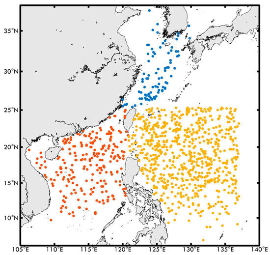
Figure 1.
Typhoon eye positions in three regions: ECS (blue), SCS (red), and WP (yellow).

Table 1.
The number of typhoon eye positions in the study area and their corresponding intensities.
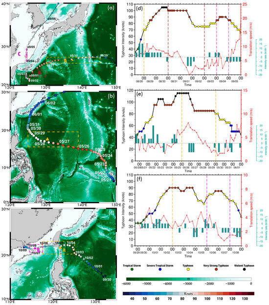
Figure 2.
Bathymetry and typhoon tracks based on the ETOPO1 dataset for (a) Hinnamnor (2022), (b) Mawar (2023), and (c) Koinu (2023). Colored dots indicate six-hourly typhoon intensity. The black contour marks the 200 m isobath. Colored boxes represent MHW regions associated with each typhoon, corresponding to time series analyses. Triangles indicate the central point of each box, averaged from time series and typhoon locations. (d–f) Typhoon intensity evolution from JMA best-track data, with colored dots indicating intensity levels from tropical depression to violent typhoons. Blue bars represent six-hourly intensity changes (knots), with positive values for intensification and negative values for weakening.
Table 2.
Summary of typhoon characteristics. Positive, negative, and zero intensity changes indicate intensification, dissipation, and maintenance.
2.2. MHWs Analysis
MHW events are defined as periods of anomalously high SST, following the criteria established by [1]. An MHW event is identified when SST at a given grid point exceeds the climatological 90th percentile for at least five consecutive days. If two events are separated by a gap of two days or less, they are considered part of a single continuous event. Daily SST anomalies are calculated by removing the corresponding daily climatology; although the commonly used MHW climatological base period is 1985–2012, to match the reanalysis data years, the 1993–2012 base period is used to determine both the anomalies and the 90th percentile threshold for MHW detection. Within the study area (105–150°E, 0–50°N), the average SST for the 1985–2012 period is 24.48 °C, while for the 1993–2012 period it is 24.58 °C. Due to the base period being slightly higher by 0.1 °C, the MHW categories may be slightly lower compared to those derived from the original climatological cycle. Once an MHW is identified, it is classified by intensity according to the method described in [30]. The categorization is based on the difference (Diff) between the average SST (Avg) and the 90th percentile value at each grid point. This system allows for a detailed assessment of MHW severity, ranging from no MHW conditions to extreme MHW events, as follows: Category 0: No MHW (SST below the 90th percentile); Category 1: Moderate (Avg + Diff ≤ SST < Avg + 2Diff); Category 2: Strong (Avg + 2Diff ≤ SST < Avg + 3Diff); Category 3: Severe (Avg + 3Diff ≤ SST < Avg + 4Diff); Category 4: Extreme (Avg + 4Diff ≤ SST < Avg + 5Diff) and Category 5: Beyond Extreme (SST ≥ Avg + 5Diff).
This study extends beyond merely identifying MHW events in the context of typhoon interactions. A comprehensive analysis characterized MHW spatiotemporal attributes using three key metrics: maximal intensity, frequency, and duration. Table 3 presents the detailed definitions of these metrics, which are essential for understanding the full scope of this study.
Table 3.
Definitions of the MHW metrics.
2.3. Oceanic and Atmospheric Parameters
The Global Ocean Physics Reanalysis product (GLORYS12V1) from the Copernicus Marine Environment Monitoring Service (CMEMS) supplies daily ocean temperature data. This dataset spans 1993 to 2023, offering a daily temporal resolution with a horizontal resolution of 1/12°, distributed across 50 uneven vertical layers (Product ID: GLOBAL_MULTIYEAR_PHY_001_030). As a global eddy-resolving ocean dataset, GLORYS12V1 is based on the Nucleus for European Modelling of the Ocean platform, with surface forcing provided by the European Centre for Medium-Range Weather Forecasts (ECMWF) ERA-Interim. Observations are integrated using a reduced-order Kalman filter. Extensive validation with in situ and satellite data ensures its reliability for detailed oceanographic research [31,32,33]. From this dataset, we obtained SST for MHW detection, MLD, and computed upper OHC and depth-average temperature.
To compare these ocean parameters with long-term climatic averages, we utilized the monthly World Ocean Atlas 2018 (WOA18) dataset produced by the National Centers for Environmental Information (NCEI) of the National Oceanic and Atmospheric Administration (NOAA). This dataset provides climatological averages and related statistics for several oceanographic variables, with a spatial resolution of 0.25°, offering valuable insights into the physical characteristics of the global ocean [34].
We used ERA5, the fifth-generation reanalysis dataset from ECMWF, for atmospheric parameters. ERA5 provides high resolution, hourly estimates of atmospheric and near-surface variables, with a spatial resolution of 0.25°. It is widely recognized for its accuracy and extensive spatial-temporal coverage, making it a valuable resource for analyzing air–sea interactions and climate dynamics [35,36]. Air–sea heat fluxes, including the combined contributions of sensible and latent heat, were derived from ERA5 reanalysis data to quantify ocean–atmosphere energy exchange.
To evaluate the impact of subsurface heat accumulation during compound extreme events involving MHWs and typhoons, we utilized the concept of upper OHC, which is defined as the vertically integrated temperature from the sea surface down to the depth of the 26 °C isotherm (D26), as formulated in Equation (1), where represents seawater density (approximately 1025 kg/m3) and denotes the specific heat capacity of seawater (approximately 4000 J/(kg°C)). Additionally, the depth-average temperature of the upper 100 m is a key parameter for assessing ocean heat content. Recognized as an effective indicator of thermal energy in the ocean’s upper layer, is computed using Equation (2), which calculates the mean temperature from the sea surface to a depth of 100 m [37].
2.4. Spatial and Temporal Analysis
The outermost radii of 30 knots (R30) and 50 knots (R50) winds from the typhoon center are identified as key regions where typhoon–ocean interactions are most intense. Using JMA best-track data, oceanic parameters—including MHW category, OHC, , MLD, and heat fluxes—are extracted and averaged at daily intervals within these radii. This approach enables a temporal assessment of oceanic responses before, during, and after typhoon passage.
The R30 and R50 radii are crucial for studying typhoon intensification, as they encompass the primary energy extraction zone, where heat fluxes, upwelling, and ocean mixing play a significant role in typhoon development. R50 represents the typhoon’s inner-core impact zone, whereas R30 provides a broader perspective on ocean–atmosphere interactions. This study systematically compares Typhoon Hinnamnor (2022), Typhoon Mawar (2023), and Typhoon Koinu (2023) to elucidate the influence of MHWs and subsurface warming on typhoon intensification and dissipation phases, with implications for improving intensity forecasting and climate resilience research.
Additionally, MHW detection domains were defined based on time series data and typhoon locations, as illustrated in Figure 2. For Typhoon Hinnamnor (2022), three domains were delineated based on typhoon intensity and bathymetry: Domain A (25.83–27.33°N, 130.3–145.3°E): 29–31 August; Domain B (22.42–24.25°N, 124.6–130.3°E): 31 August–3 September; and Domain C (26.33–29.42°N, 124.6–124.9°E): 4–5 September. Triangles represent the center points of each domain, computed as the average typhoon position (longitude and latitude) over the specified period. The latitudinal extent of each domain was defined within R50 from the center point, ensuring that each domain fully captures the typhoon’s impact area. Similarly, for Typhoon Mawar (2023), the analysis spans 26–30 May, covering the domain (15.58–19.5°N, 125.1–139.2°E). For Typhoon Koinu (2023), the study is divided into two domains: Domain A (20.25–23.00°N, 117.7–125.1°E): 3–6 October and Domain B (20.67–22.33°N, 114.6–117.7°E): 6–8 October.
3. Results
3.1. Dual Effects of MHWs on Typhoon Intensity and Associated Heat Dissipation
Based on 1027 typhoon position cases from 1993 to 2023, the results indicate that regardless of region, typhoon intensity, or typhoon intensity change, the MHW category remained at a relatively high level from Day −7 to Day 0 but generally exhibited a significant decline after typhoon passage, highlighting the substantial impact of typhoons in disrupting MHWs. Stronger typhoons and those that interact with MHWs for an extended duration tend to accelerate the dissipation of MHWs in both magnitude and speed (Figure 3). Figure 3a illustrates regional differences in MHW categories on Day −7, with the SCS exhibiting the highest values, averaging between 0.45 and 0.5, whereas the WP had relatively lower values. This suggests that, at the same time, the MHWs in the WP were not as pronounced as in the SCS. However, regardless of the region, the MHW category dropped significantly upon typhoon arrival and passage (Day 0 to Day 1), indicating that strong wind stress and ocean mixing associated with typhoons disrupt or weaken MHWs. Heat accumulation in semi-enclosed seas such as the SCS and ECS is more pronounced during MHW formation, leading to higher MHW intensity. However, once a typhoon passes, the disruptive effects are also more severe. As a vast and more complex oceanic region, the WP exhibits a lower average MHW intensity than the SCS but follows a similar dissipation trend. Figure 3b shows that the decline in MHW categories after typhoon passage (Day 0 to Day 1) is particularly pronounced for Violent and Very Strong typhoons, suggesting that stronger typhoons induce significant vertical mixing, upwelling, and cold-water entrainment, leading to the rapid dissipation of MHWs. While weaker typhoons (Severe Tropical Storm and Typhoon) also contribute to MHW reduction, the extent of the decline is relatively smaller. Additionally, stronger typhoons are often associated with higher pre-existing MHW conditions, possibly contributing to their intensification. Figure 3c indicates that, regardless of whether a typhoon intensifies or weakens during its lifecycle, MHWs will likely experience some degree of disruption. However, typhoons that maintain their intensity appear to have a more pronounced impact on MHW dissipation, suggesting that prolonged interaction with MHWs may enhance their destruction.
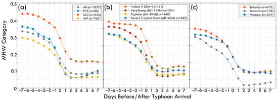
Figure 3.
Changes in MHW category before and after typhoon passage: (a) Different regions, (b) Different typhoon intensities, and (c) Different typhoon intensity changes.
Figure 4a presents a scatter plot illustrating the distribution of typhoon intensity rate and MHW category, complemented by box plots that depict the statistical characteristics across different intensity rate intervals and oceanic regions (Figure 4b–e). The results indicate that some intensifying typhoons in the SCS correspond to higher MHW categories, whereas in the WP, although the typhoon intensity rate exhibits a broader distribution, the highest MHW categories are less frequent compared to the SCS. Overall, there is no monotonic or linear relationship between typhoon intensity rate and MHW category. Specifically, a greater increase in typhoon intensity does not necessarily correspond to a higher MHW category, nor does a greater decrease in intensity always correspond to a lower MHW category. Instead, the data exhibit a dispersed distribution.
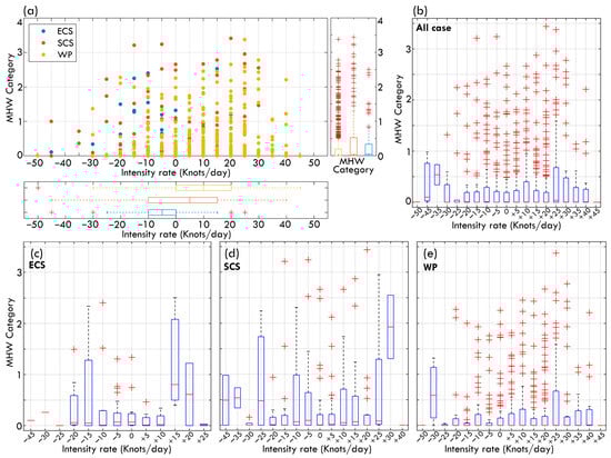
Figure 4.
Analysis of typhoon intensity rate with MHW category. (a) Scatter plot showing the relationship between typhoon intensity rate (knots/day) and MHW category for ECS, SCS, and WP. Boxplots of intensity rate and MHW category are overlaid at the bottom and right side. (b) Boxplots summarizing all cases of typhoon intensity rate change vs. MHW Category. (c–e) same as (b) but for ECS, SCS, WP only.
The box plots provide additional insights into the median, interquartile range, and outliers, highlighting that even within the same intensity rate interval or oceanic region, some typhoons experienced significantly high MHW categories. For example, high MHW categories in the ECS are predominantly concentrated in low to moderate-intensity change rates (within ±10 knots/day), with some extreme outliers. In contrast, in the SCS, higher MHW categories are observed more frequently when typhoons intensify significantly (>10 knots/day), suggesting that MHWs may persist at higher levels in this region during rapid typhoon intensification. Conversely, the WP exhibits a more dispersed distribution of MHW categories, with high MHW outliers occurring across various intensity rate intervals. However, the median MHW category remains relatively low. While the median results suggest that MHW categories tend to be higher when typhoons intensify, it remains unclear whether high MHWs directly contribute to typhoon intensification or whether typhoons intensify while passing through high MHW regions. The interaction between typhoons and MHWs may be bidirectional. This highlights the necessity of incorporating additional spatiotemporal factors, such as OHC, ocean stratification, and atmospheric conditions during typhoon passage, to better elucidate causal relationships and mechanisms of intensification or dissipation. The next section examines three representative typhoon case studies to further explore the complexity of typhoon–ocean interactions.
3.2. Interaction Between MHWs and Typhoons: Case Study
An analysis of MHW frequency, duration, and intensity during 2022 and 2023 reveals significant interactions with Typhoons Hinnamnor (2022), Mawar (2023), and Koinu (2023) (Figure 5). In 2022, MHW frequency exceeded 10 events in the Kuroshio Current and adjacent marginal seas, particularly in the ECS and NWP (Figure 5a). MHW duration exhibited substantial spatial variability (Figure 5b), with prolonged events (>40 days) concentrated in the Kuroshio Current, reinforcing its role as a thermal hotspot. Along Hinnamnor’s track, MHW durations were shorter (5–25 days), indicating more transient warm anomalies. In 2023, MHW frequency exceeded 10 events in the SCS (Figure 5d). MHW duration varied significantly across regions (Figure 5e); the two typhoons experienced slightly shorter MHW durations along their paths near Taiwan, with the longest durations (30–40 days) observed in the NWP near the equator. In the marginal SCS, MHW duration was shorter (10–15 days) but increased to 20–40 days in specific areas. MHW intensity, represented by the highest SST anomaly (°C), exhibited distinct regional variations in both years (Figure 5c,f), further emphasizing the spatial complexity of MHW–typhoon interactions.
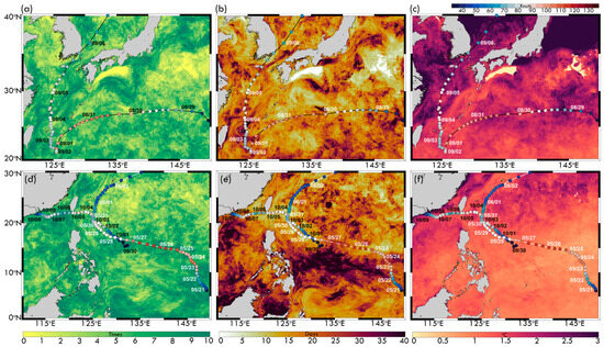
Figure 5.
Spatial distribution of (a,d) MHW frequency, (b,e) MHW duration, and (c,f) MHW maximum intensity. Panels (a–c) correspond to 2022, overlaid with Typhoon Hinnamnor’s track (29 August–06 September). Panels (d–f) correspond to 2023, showing the tracks of Typhoon Mawar (21 May–2 June, white curve) and Typhoon Koinu (30 September–09 October, black curve).
3.2.1. Typhoon Hinnamnor (2022) and Its Interaction with MHWs
Typhoon Hinnamnor (2022), which formed on 29 August, exhibited two intensification phases (Figure 2a). The first phase (29–30 August) peaked at 105 knots before weakening (31 August–3 September) in Domain B. The second intensification (4 September) occurred as the typhoon entered the ECS, reaching 90 knots. These fluctuations reflect the varying oceanic conditions along its path. Figure 6a–c illustrate MHW activity within these domains, strongly aligning with Hinnamnor’s intensity changes. In Domain A (Figure 6a), SST remained above the 90th percentile during the first intensification, reaching 30.5 °C. As Hinnamnor strengthened, typhoon-induced mixing and upwelling caused slight SST cooling, but MHW conditions persisted. In Domain B (Figure 6b), as Hinnamnor weakened, SST dropped from 30.5 °C to 29.8 °C (below the 90th percentile) by 3 September, indicating MHW dissipation due to prolonged ocean mixing. In Domain C (Figure 6c), during the second intensification phase (4 September), SST recovered to ~30 °C, maintaining Category 1 MHW conditions. This re-establishment of warm waters in the ECS likely contributed to Hinnamnor’s re-intensification, underscoring the role of regional thermal anomalies in modulating typhoon evolution.
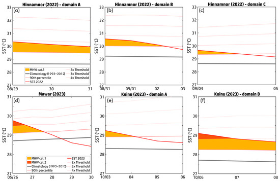
Figure 6.
Time series and intensity of MHW events associated with three typhoons: (a–c) Typhoon Hinnamnor (2022) in Domains A (25.83–27.33°N, 130.3–145.3°E), B (22.42–24.25°N, 124.6–130.3°E), and C (26.33–29.42°N, 124.6–124.9°E); (d) Typhoon Mawar (2023) within 15.58–19.5°N, 125.1–139.2°E; (e,f) Typhoon Koinu (2023) in Domains A (20.25–23.00°N, 117.7–125.1°E) and B (20.67–22.33°N, 114.6–117.7°E). Domain locations correspond to Figure 2.
Figure 7a illustrates the spatial evolution of MHW intensity (Categories 1–2) from 29 August to 5 September, overlaid with Hinnamnor’s track. These maps reveal how MHWs dynamically responded to the typhoon. From 29 to 31 August, Category 1 MHWs dominated along the track, particularly near the Kuroshio Current, where persistent SST anomalies likely fueled Hinnamnor’s first intensification phase. Between 1 and 3 September, MHW intensity declined, especially on 2–3 September, due to typhoon-induced mixing and upwelling, which disrupted surface warming. By 4–5 September, as Hinnamnor entered the ECS, MHW intensity strengthened to Category 2, particularly near the ECS and Kuroshio Current, supporting Hinnamnor’s second intensification. Overall, Figure 7a highlights the strong influence of MHWs on Hinnamnor’s evolution, especially during its two intensification phases. Conversely, Hinnamnor-induced cooling (Figure 6a–c and Figure 7a) led to SST declines and MHW weakening along the track. However, SST gradually recovered, with MHW Categories 1–2 persisting in the ECS, facilitating Hinnamnor’s re-intensification.
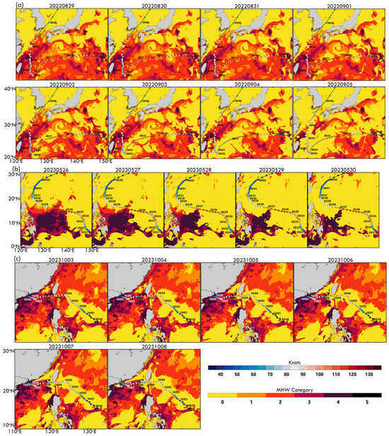
Figure 7.
Daily MHW category maps showing the spatial distribution of MHWs during typhoon events: (a) Hinnamnor (2022) from 29 August to 5 September, (b) Mawar (2023) from 25 May to 30 May, and (c) Koinu (2023) from 3 October to 8 October. Each panel corresponds to the domains identifying MHWs in the respective typhoon tracks.
Figure 8a,b present the MHW category time series (±7 days around Hinnamnor’s arrival) within R30 and R50, illustrating typhoon-induced cooling effects. Before Hinnamnor’s arrival (Days −7 to −1), MHW categories remained high in both regions, indicating elevated SST and strong pre-existing ocean heat content. On Day 0, as Hinnamnor arrived, MHW categories declined sharply, effectively suppressing MHW effects in most areas. One exception occurred on 29–30 August, when Hinnamnor intensified to 95–90 knots. During this period, MHW conditions persisted, though their category dropped from 2 to 1, suggesting that SST remained warm enough to sustain lower-intensity MHWs despite typhoon-induced mixing. Post-typhoon, MHW responses differed spatially. Within R50 (near-inner core), MHW categories dropped rapidly on Days 1–2, indicating a more substantial and immediate impact of mixing and upwelling near the typhoon’s center. In contrast, within R30 (outer core), MHW categories declined gradually between Days 2–4, reflecting a slower and more persistent cooling effect. This distinction underscores the spatial variability of MHW responses, where rapid cooling dominated the inner core (R50), while gradual cooling characterized the outer core (R30).
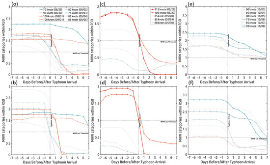
Figure 8.
Time series of MHW categories ±7 days before and after typhoon arrival within R30 (a,c,e) and R50 (b,d,f). Panels show results for (a,b) Hinnamnor (2022), (c,d) Mawar (2023), and (e,f) Koinu (2023). Colored curves represent typhoon intensity, corresponding to the scale in the color bar.
3.2.2. Typhoon Mawar’s Evolution and MHW Interaction
While Typhoon Hinnamnor (2022) demonstrated how pre-existing MHWs can fuel typhoon intensification, Typhoons Mawar (2023) and Koinu (2023) exhibited more complex interactions, where intensity varied significantly or was suppressed, highlighting the intricate interplay between oceanic and atmospheric factors. Mawar formed on 21 May and peaked at 115 knots on 26 May before rapidly weakening from 27 May onward (Figure 2b,e). To investigate this decline, MHW conditions along Mawar’s track (26–30 May) were analyzed (Figure 2b,e and Figure 6d). On 26 May, SST exceeded the 90th percentile, sustaining Category 1 MHW conditions (dark yellow shading) and localized Category 2 (dark orange shading), providing favorable oceanic heat for Mawar’s peak intensity. However, as Mawar progressed, SST dropped sharply from ~30 °C on 26 May to below 29 °C by 30 May, coinciding with a significant reduction in MHW intensity. By 28 May, SST fell below the 90th percentile, effectively eliminating MHW conditions. This cooling was driven by typhoon-induced vertical mixing and upwelling, disrupting the warm surface layer and bringing cooler subsurface waters to the surface. Mawar’s intensity dropped from 115 knots on 26 May to 80 knots on 30 May. The decline in SST and MHW coverage, alongside possible changes in wind shear and mid-level moisture, likely contributed to its weakening. These findings emphasize MHWs as key energy sources for typhoon intensification, while ocean–atmosphere feedbacks—such as mixing and upwelling—play a crucial role in modulating typhoon evolution.
Figure 7b illustrates the daily evolution of MHW categories from 26 May to 30 May, revealing how MHW conditions changed under Mawar’s track during its weakening. On 26 May, when Mawar peaked at 115 knots, Category 1 and localized Category 2 MHW conditions were present along its track, particularly in the NWP, suggesting that pre-existing SST anomalies contributed to its intensification. However, by 27–28 May, MHW spatial coverage and intensity declined noticeably as typhoon-induced mixing and upwelling disrupted ocean heat content. By 29–30 May, MHWs along Mawar’s track had mainly dissipated, with SST falling below the MHW threshold, coinciding with Mawar’s weakening from 105 knots on 27 May to 80 knots on 30 May. The gradual decline in MHW intensity and coverage underscores the dynamic interaction between Mawar and the underlying ocean heat reservoir, where typhoon-induced cooling reduces the availability of warm ocean heat, leading to progressive weakening.
Figure 8c,d show MHW time series (±7 days) within R30 and R50, illustrating Mawar’s interaction with pre-existing warm anomalies. In R30, MHW categories remained high (Category 1–2) for seven days before Mawar’s arrival (Days −7 to −1), sustaining its peak intensity of 115 knots on 26 May. However, post-arrival (Day 0), MHWs rapidly declined, falling below the threshold (no MHWs) by Day +2, due to vigorous vertical mixing and upwelling, leading to sustained ocean cooling. Unlike R30, MHWs in R50 persisted slightly longer, but declined more gradually, falling below the threshold by Day +3. Partial MHW recovery was observed from Day +4 onward, with Category 1 conditions re-emerging by Day +7, suggesting the faster recovery in R50 due to reduced cooling effects near the typhoon’s inner core. These findings emphasize the critical role of pre-existing MHWs in fueling Mawar’s intensification and the strong ocean–atmosphere feedback mechanisms—particularly mixing and upwelling—that drive rapid SST cooling and spatially variable MHW recovery.
3.2.3. Typhoon Koinu’s Evolution and MHW Interaction
Typhoon Koinu (2023) exhibited significant intensity variations, reaching a peak of 90 knots on 3–4 October before rapidly weakening within 12 h on both days. Between 3 October and 6 October, Koinu’s intensity dropped from 90 knots to 75 knots. Upon entering the marginal sea of the SCS, it briefly re-intensified to 85 knots on 7 October before experiencing another gradual decline (Figure 2c,f). To investigate the mechanisms behind these intensity fluctuations, we analyzed MHW conditions along Koinu’s track from 3 October to 6 October (Domain A) and 6 October to 8 October (Domain B) (Figure 2c,f). The time series of MHW events along Koinu’s path (Figure 6e,f) reveals key interactions between MHW conditions and typhoon evolution. In Domain A (3 October, Figure 6e), SSTs exceeded the 90th percentile, supporting Category 1 MHW conditions (dark yellow shading) and providing sufficient heat for Koinu’s peak intensity. However, from 4 October onward, SST declined rapidly, dropping from above 29 °C to ~28.°C by 6 October. This cooling coincided with a sharp reduction in MHW coverage and intensity, as SSTs fell below the 90th percentile threshold. The SST decline was likely driven by typhoon-induced vertical mixing and upwelling, disrupting the warm surface layer and reducing the available thermal energy needed to sustain Koinu’s intensity. Consequently, Koinu weakened by 15 knots over three days. Figure 6e illustrates the dynamic interplay between Koinu and MHW conditions, demonstrating that pre-existing warm SSTs initially supported intensification, but rapid SST cooling and weakened MHW conditions contributed to its decline. These findings highlight the crucial role of ocean–atmosphere feedback mechanisms, such as mixing and upwelling, in regulating typhoon evolution.
As Koinu moved into the marginal sea of the SCS (Domain B) from 6 October to 8 October, stronger MHW conditions (Categories 1–2) were observed (Figure 2c,f and Figure 6f). Elevated SSTs (>28 °C) and persistent thermal anomalies (dark orange shading) provided sufficient energy for Koinu’s second intensification. During this period, SSTs remained above the critical threshold for typhoon maintenance, peaking near 29 °C on 6 October before gradually cooling by 8 October due to typhoon-induced mixing and upwelling. This SST decline underscores the strong feedback between Koinu and ocean dynamics, where the typhoon extracted heat from the shallow SCS waters, contributing to its re-intensification. The limited heat storage capacity of shallow seas made them more susceptible to rapid SST fluctuations, reinforcing the role of MHWs in amplifying typhoon strength under favorable conditions while also being vulnerable to dissipation through typhoon-induced processes.
The daily MHW category maps (Figure 7c, 3–8 October) illustrate the evolution of MHWs along Koinu’s trajectory, revealing significant spatial variations in intensity (Categories 1–4) across the SCS and adjacent regions. From 3 October to 5 October, Koinu traversed moderate MHW areas (Categories 1–2) in the western SCS, where pre-existing warm anomalies provided the thermal energy necessary for intensification. On 3 October, as Koinu reached peak intensity (90 knots), localized Category 1 and 2 MHWs were prominent, particularly in the NWP and northern SCS. However, MHW coverage declined by 4 October, as typhoon-induced mixing and upwelling disrupted MHW extent and intensity, coinciding with Koinu’s weakening. By 5 October, further MHW dissipation aligned with Koinu’s intensity drops to 80 knots. Starting 6 October, a pronounced increase in MHW intensity (Categories 2–3) appeared in the shallow SCS, aligning with Koinu’s second intensification phase. Thermal hotspots formed along Koinu’s track on 7 and 8 October, with Category 3 MHWs in localized areas, likely influenced by warm water advection and shallow bathymetry. Despite high MHW intensities, Figure 7c indicates a progressive cooling trend along Koinu’s trajectory, emphasizing the competing effects of MHW-fueled intensification and typhoon-induced dissipation. This is particularly evident after 6 October, as Koinu moved through more substantial MHW regions. These results highlight the crucial role of pre-existing warm anomalies in supporting intensification while also demonstrating how typhoon-induced ocean processes gradually weaken MHWs.
The time series of MHW categories (±7 days around Koinu’s arrival, Figure 8e,f) illustrates temporal variations in MHW intensity within R30 and R50. Before Koinu’s arrival, MHW categories consistently exceeded Category 1, peaking at Category 2, providing favorable thermal conditions for intensification. The figures reveal two distinct phases of MHW–typhoon interaction. From 3 October to 6 October, as Koinu weakened, MHW categories remained between 1 and 2, with R50 briefly reaching Category 3, suggesting stronger localized thermal anomalies near the typhoon’s core, while R30 remained stable. After Koinu’s arrival (Day 0), a sharp decline in MHW categories followed, driven by typhoon-induced vertical mixing and upwelling, which disrupted oceanic heat availability. In R30, MHW reduction was gradual, stabilizing around Category 1 post-typhoon. In R50, MHW categories dropped rapidly after 3 October, falling below Category 1 the day after the typhoon’s passage, followed by a slower decline from 6 October to 8 October, decreasing from Category 2 to 1 by Day 7. These patterns highlight MHW responses’ spatial and temporal variability, reinforcing the complex interplay between typhoon dynamics and ocean heat anomalies.
3.3. Role of Subsurface Temperature and Heat Content: Case Study
3.3.1. Subsurface Ocean Characteristics During Typhoon Hinnamnor (2022) Development
While surface conditions drive typhoon intensification, subsurface ocean heat plays a crucial role in MHW-typhoon interactions. Figure 9a illustrates daily OHC variations along Typhoon Hinnamnor’s track (29 August–5 September), highlighting key ocean-typhoon energy exchanges. High OHC (100–160 kJ/cm2), concentrated along the Kuroshio Current and adjacent marginal seas, provided a critical energy source. From 29 August to 31 August, Hinnamnor traversed moderate OHC regions (50–150 kJ/cm2), reaching peak intensity (100 knots) on August 30. Despite an increase in OHC from 31 August to 4 September, particularly in the ECS, the typhoon weakened before briefly re-intensifying on 4–5 September as it moved over elevated OHC zones. By 5 September, OHC significantly declined along Hinnamnor’s path due to typhoon-induced vertical mixing and upwelling, redistributing subsurface heat. These findings underscore the complex interplay between typhoons and ocean heat reservoirs, where pre-existing warm waters can enhance intensification, but mixing effects deplete thermal energy. The Kuroshio Current, a key high-OHC region, strongly supports typhoon growth and heightened susceptibility to heat loss following typhoon passage.
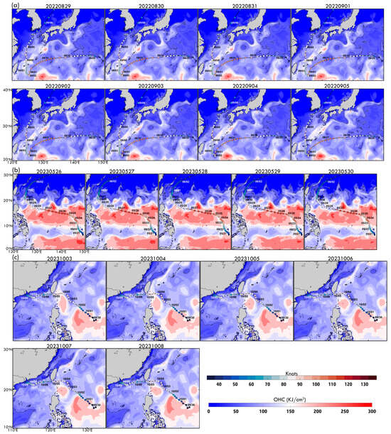
Figure 9.
Daily OHC category maps for (a) Hinnamnor (2022) from 29 August to 5 September, (b) Mawar (2023) from 25 May to 30 May, and (c) Koinu (2023) from 3 October to 8 October. Each typhoon’s time series aligns with the corresponding MHW domains.
The time series of OHC (±7 days before and after Hinnamnor’s arrival) within R30 and R50 (Figure 10a,b) further illustrates the role of subsurface heat. Before arrival (Days −7 to −1), OHC remained stable, with R50 exhibiting slightly higher values (100–120 kJ/cm2) than R30 (90–110 kJ/cm2), providing a crucial heat reservoir that fueled Hinnamnor’s intensification, peaking at 100 knots on 31 August. After arrival (Day 0), typhoon-induced mixing and upwelling caused a sharp OHC decline. In R30, reductions were moderate except on 31 August, when OHC dropped below 100 kJ/cm2. In contrast, R50 experienced a more substantial decline (60–100 kJ/cm2), particularly on 31 August and 3 September. The stronger heat loss in R50 highlights spatial variability in typhoon–ocean interactions, emphasizing the localized nature of subsurface heat depletion and its role in shaping Hinnamnor’s intensity fluctuations.
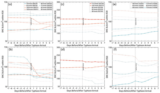
Figure 10.
Time series of OHC ±7 days before and after typhoon arrival within R30 (a,c,e) and R50 (b,d,f). (a,b) Hinnamnor (2022), (c,d) Mawar (2023), and (e,f) Koinu (2023). Colored curves indicate typhoon intensity, following the color bar scale.
Figure 11a illustrates daily maps (29 August–5 September), showing subsurface temperature variations along Hinnamnor’s track. Figure 12a,b present the time series of within R30 and R50, highlighting its relationship with typhoon intensity. On 29 August, during Hinnamnor’s intensification, exceeded 29 °C, particularly near the Kuroshio Current and within R50, serving as a crucial energy source. The pre-arrival period (Days −7 to −1) exhibited stable (~29 °C) in both regions, supporting Hinnamnor’s development. Upon arrival (Day 0), typhoon-induced mixing and upwelling caused a significant temperature drop. In R50, fell sharply below 28 °C and continued declining toward 27 °C. In R30, the decline was more gradual, with temperatures remaining above 27 °C for longer. These subsurface cooling trends coincided with Hinnamnor’s weakening phase as it moved northward. The combination of daily maps and time series underscores the key role of subsurface temperatures in regulating typhoon intensity. Elevated pre-arrival facilitated intensification, while post-arrival cooling via mixing and upwelling limited further strengthening. The more pronounced cooling in R50 highlights subsurface thermal conditions’ spatial and temporal variability in shaping typhoon behavior.
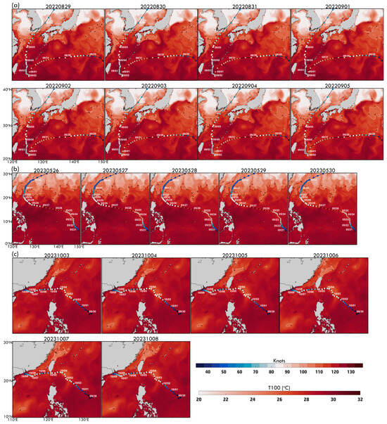
Figure 11.
Daily maps illustrating subsurface temperature distribution during typhoon events: (a) Hinnamnor (2022) from 29 August to 5 September, (b) Mawar (2023) from 25 May to 30 May, and (c) Koinu (2023) from 3 October to 8 October. Time series correspond to the identified MHW domains.
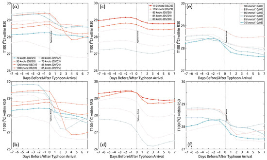
Figure 12.
Time series of ± 7 days before and after typhoon arrival within R30 (a,c,e) and R50 (b,d,f): (a,b) Hinnamnor (2022), (c,d) Mawar (2023), and (e,f) Koinu (2023). Colored curves represent typhoon intensity, corresponding to the color scale.
3.3.2. Subsurface Ocean Characteristics During Typhoon Mawar (2023) Development
The daily OHC maps from 26 May to 30 May (Figure 9b) illustrate the relationship between OHC and Typhoon Mawar’s intensity. At its peak (115 knots, 26 May), OHC exceeded 300 kJ/cm2, providing a subsurface heat reservoir. However, OHC steadily declined below 150 kJ/cm2 by 27 May, coinciding with Mawar’s weakening. This downward trend continued until the typhoon dissipated, highlighting how vertical mixing and upwelling depleted subsurface heat, ultimately contributing to the typhoon’s weakening. The OHC time series (±7 days, Figure 10c,d) further clarifies these processes. Before arrival (Days −7 to −1), R50 consistently exhibited higher OHC (~200 kJ/cm2) than R30 (~190 kJ/cm2), supporting Mawar’s intensification. After arrival (Day 0), OHC declined due to mixing and upwelling, with R30 dropping below 150 kJ/cm2 by Day +7, reflecting substantial heat loss near the core. In R50, OHC followed a similar decreasing trend but remained slightly higher, highlighting spatial variability in typhoon-induced subsurface heat depletion. This continuous decline in OHC aligned with Mawar’s weakening to 80 knots by 30 May, emphasizing the balance between pre-existing subsurface heat sustaining intensification and post-typhoon ocean–atmosphere interactions limiting further development.
Figure 11b presents daily maps from 26 May to 30 May, illustrating subsurface temperature variations along Mawar’s track. Figure 12c,d show the corresponding time series within R30 and R50, revealing how subsurface heat evolved relative to typhoon intensity. At peak intensity (115 knots, 26 May), exceeded 29 °C in both R30 and R50, particularly in the NWP, providing essential thermal energy for intensification. Before arrival (Days −7 to −1), remained stable, with R50 (~29.5 °C) slightly higher than R30 (~29 °C), reflecting stronger heat retention near the inner core. After arrival (Day 0), typhoon-induced vertical mixing and upwelling led to a decline in . In R30, fell below 28 °C by Day +7, indicating substantial heat loss in the outer core. In R50, it dropped gradually to ~27.5 °C by Day +3, stabilizing at ~27 °C by Day +7, suggesting less heat depletion near the inner core. As Mawar weakened, continued to decline, reinforcing the link between subsurface heat loss and typhoon weakening. The disparity between R30 and R50 highlights the localized impacts of typhoon–ocean interactions, with more significant thermal disruption in the outer-core region. This analysis underscores the crucial role of in Mawar’s lifecycle: pre-arrival elevated values supported peak intensity, while post-arrival cooling, particularly in R50, contributed to weakening as Mawar’s intensity dropped to 80 knots by 30 May. These findings emphasize subsurface thermal structure as a key factor in modulating typhoon behavior.
3.3.3. Subsurface Ocean Characteristics During Typhoon Koinu (2023) Development
For Typhoon Koinu (2023), daily OHC maps (3–8 October, Figure 9c) show elevated OHC (>150 kJ/cm2) supporting its peak intensity of 90 knots on 3 October, particularly east of the Philippines and in the NWP. These high OHC values sustained intensification. However, from 4 October to 6 October, OHC steadily declined due to typhoon-induced vertical mixing and upwelling, though localized areas of elevated OHC persisted in the SCS, aiding Koinu’s secondary intensification. By 8 October, OHC had dropped below 100 kJ/cm2 across most regions, reflecting subsurface heat depletion as Koinu weakened. The time series of OHC (±7 days before and after Koinu’s arrival) within R30 and R50 (Figure 10e,f) further illustrates subsurface heat evolution. Before arrival (Days −7 to −1), OHC remained stable, with R50 (~130–150 kJ/cm2) slightly higher than R30 (~120–140 kJ/cm2), providing the energy needed for Koinu’s peak intensity on 3 October. After arrival (Day 0), OHC steadily declined due to vertical mixing and upwelling. Within R30, OHC fell to ~70–100 kJ/cm2 by Day +7, reflecting moderate heat depletion in the outer region. In R50, the decline was more rapid, with OHC dropping to 50–115 kJ/cm2, indicating significant heat loss near the typhoon’s core. Even during Koinu’s re-intensification on 7 October (85 knots), OHC continued to decline below 100 kJ/cm2, and its intensity ultimately decreased to 70 knots by 8 October. These findings highlight OHC’s critical role in fueling typhoon intensification while underscoring the feedback mechanisms that deplete subsurface heat, ultimately contributing to Koinu’s weakening.
Figure 11c presents daily maps (3–8 October), illustrating subsurface temperature variations along Koinu’s track, while Figure 12e,f show the time series within R30 and R50, highlighting thermal evolution relative to typhoon intensity. On 3 October, when Koinu peaked at 90 knots, exceeded 28.5 °C in both regions, providing essential energy for intensification, particularly in the SCS and WP. During the pre-arrival phase (Days −7 to −1), remained stable, with slightly higher values in R50 (~27.8–29.2 °C) than R30 (~27.2–29 °C), consistent with stronger thermal retention near the typhoon’s core. After Koinu’s arrival (Day 0), declined due to vertical mixing and upwelling, redistributing and reducing subsurface heat. In R30, gradually dropped to ~27.5–28.5 °C by Day +7, while R50 showed a more rapid decline, reaching 27.5–28 °C within the first two days post-typhoon. Despite Koinu’s re-intensification over the shallow SCS, continued to decrease, suggesting insufficient subsurface heat to sustain further intensification. These findings underscore the role of subsurface thermal conditions in shaping typhoon behavior and highlight the impacts of typhoon-induced processes on subsurface heat distribution.
3.4. Role of Ocean Stratification: Case Study
3.4.1. Ocean Stratification During Typhoon Hinnamnor (2022) Development
Figure 13a presents the three-day temperature profiles before Typhoon Hinnamnor’s arrival (29 August–5 September) within R30 (outer core) and R50 (near-inner core). Surface temperatures were consistently higher in R50 (~30.5 °C on 29 August, cooling to ~29 °C by 5 September) than in R30 (~30 °C to ~28 °C), reflecting stronger heat retention in the inner core. The thermocline was sharper and more localized in R50 (~50–150 m), while in R30, it extended deeper (~50–200 m), indicating greater stratification near the typhoon’s core. Cooling trends also differed: In R50, surface cooling was minor, but subsurface layers (100–200 m) exhibited greater heat loss (~1–2 °C). In R30, surface cooling was more substantial (~2 °C), while deeper layers showed less change. By 5 September, the thermocline in R50 had flattened, with temperatures at 200 m decreasing to ~21.5 °C, while in R30, it remained broader and less steep (~22 °C). These patterns suggest stronger vertical mixing and upwelling in R50, sustaining Hinnamnor’s intensity while disrupting subsurface heat reservoirs.
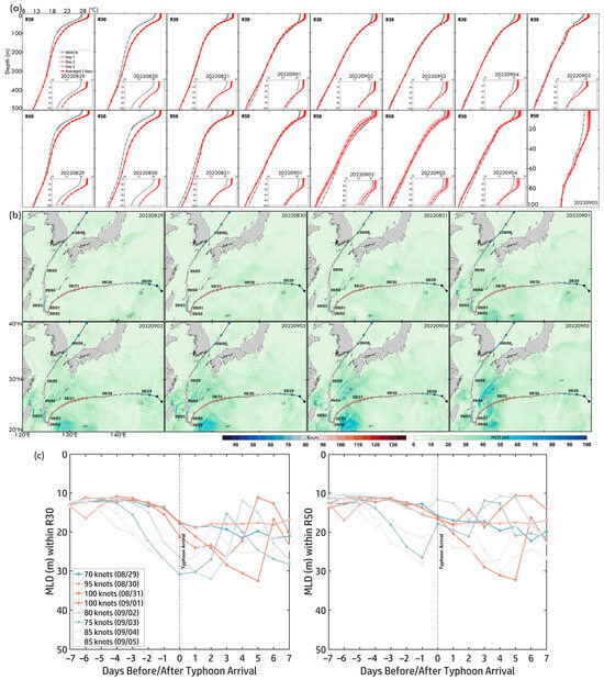
Figure 13.
(a) Three-day pre-temperature profiles within R30 and R50 along Typhoon Hinnamnor (2022) from 29 August to 5 September. Light red curves represent daily temperature profiles, while red curves indicate the three-day averaged temperature profiles. Gray curves show the monthly temperature profiles from WOA18. (b) Daily MLD maps from 29 August to 5 September. (c) Time series of MLD ±7 days before and after Hinnamnor’s arrival within R30 and R50. Colored curves correspond to the typhoon intensity scale.
Daily MLD maps (Figure 13b,c) illustrate how stratification evolved. On 29 August, MLD was shallow, favoring intensification. From 31 August to 4 September, MLD deepened significantly due to typhoon-induced mixing, reaching ~35 m in R30 and ~30 m in R50 on 5 September. After the typhoon, MLD gradually returned to pre-storm levels. The time series of MLD (±7 days around Hinnamnor’s arrival) shows stable pre-typhoon conditions, with R50 exhibiting shallower MLD (~10–15 m) than R30 (~15–20 m). Post-arrival, rapid MLD deepening reflected strong vertical mixing and a gradual recovery. These findings highlight the role of ocean stratification in modulating typhoon-ocean interactions, where stronger stratification near the inner core influences intensification, while enhanced mixing in the outer core contributes to heat loss.
3.4.2. Ocean Stratification During Typhoon Mawar (2023) Development
Figure 14a presents the three-day temperature profiles within R30 (outer core) and R50 (near-inner core) from 26 May to 30 May, illustrating subsurface thermal structure changes during Mawar’s peak intensity and subsequent weakening. Surface temperatures in R50 remained higher (~30.5 °C on 26 May, cooling to ~30 °C by 30 May) than in R30 (~30 °C to ~29.5 °C), indicating stronger heat retention in the inner core. The thermocline was steeper and more localized in R50 (~50–150 m, dropping to ~24 °C at 150 m), whereas in R30, it extended deeper (~50–200 m, declining gradually to ~23 °C). Over three days, both regions showed thermocline weakening, more pronounced in R30, indicating stronger mixing and upwelling in the outer core. Below 150 m, subsurface cooling was minimal, with R50 retaining slightly higher temperatures, reinforcing its thermal resilience and heat storage capacity. These findings suggest that R50 sustained Mawar’s peak intensity, while R30 experienced greater surface cooling and subsurface mixing, underscoring the spatial variability in typhoon–ocean interactions.
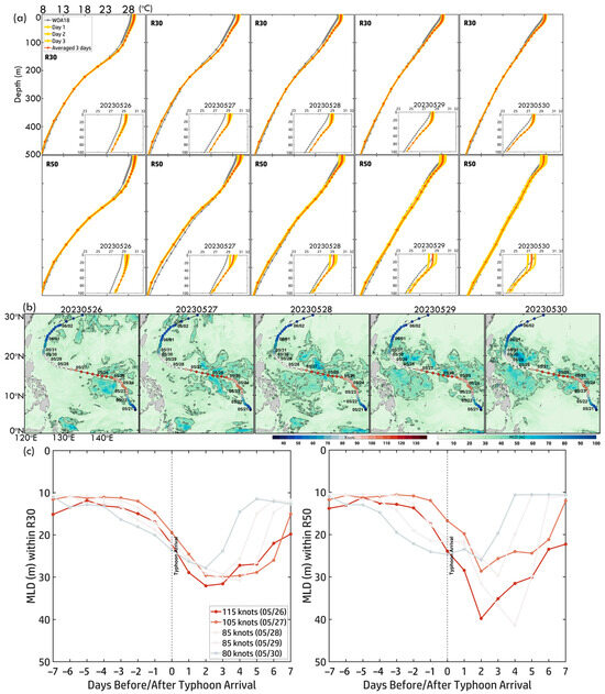
Figure 14.
(a) Three-day pre-temperature profiles within R30 and R50 along Typhoon Mawar (2023) from 26 May to 30 May. Light red curves represent daily temperature profiles, while red curves indicate the three-day averaged temperature profiles. Gray curves show the monthly temperature profiles from WOA18. (b) Daily MLD maps from 26 May to 30 May. (c) Time series of MLD ±7 days before and after Mawar’s arrival within R30 and R50. Colored curves correspond to the typhoon intensity scale.
Figure 14b,c illustrate daily MLD maps and the 7-day time series before and after Mawar’s arrival, showing significant upper-ocean responses. On 26 May, MLD was shallow (~30–50 m), particularly in the NWP, concentrating heat near the surface and favoring intensification. As Mawar weakened on 27 May, MLD deepened due to typhoon-induced mixing and upwelling, reaching ~50–70 m by 28 May. By 30 May, with Mawar at 80 knots, MLD reached its deepest levels (~70–90 m), particularly in regions exposed to prolonged strong winds. The time series shows that before Mawar’s arrival, MLD remained stable (~10–20 m), reflecting minimal pre-typhoon disturbances. Upon Mawar’s arrival, MLD deepened sharply (~40 m in R50, slightly deeper than ~35 m in R30), indicating stronger mixing near the typhoon’s core. Post-arrival, MLD remained elevated, gradually stabilizing as the typhoon dissipated. These observations highlight the role of stratification in modulating typhoon–ocean interactions. A shallow pre-typhoon MLD facilitated intensification by concentrating heat near the surface, while post-arrival deepening due to mixing and upwelling disrupted ocean thermal structure, contributing to Mawar’s weakening. Differences between R30 and R50 highlight localized variations in mixing intensity, with stronger impacts in the inner core.
3.4.3. Ocean Stratification During Typhoon Koinu (2023) Development
Figure 15a presents temperature profiles within R30 (outer core) and R50 (near-inner core) from 3 October to 8 October, illustrating subsurface thermal structure evolution during Koinu’s peak intensity and subsequent weakening. Surface temperatures in R50 remained higher (~29.8 °C on 3 October, cooling to ~29.5 °C by 8 October) than in R30 (~29.5 °C initially, decreasing by ~0.5 °C), suggesting stronger heat retention in the inner core while the outer core experienced greater cooling due to enhanced mixing. The thermocline was steeper in R50 (~50–150 m, dropping to ~24 °C at 150 m), indicating stronger stratification, while in R30, it extended deeper (~50–200 m, declining gradually to ~23 °C at 200 m). Both regions exhibited thermocline weakening due to typhoon-induced vertical mixing and upwelling, but the effect was more pronounced in R30, where heat was redistributed into deeper layers. Below 150 m, temperatures remained stable, closely aligning with climatological baselines (WOA18), indicating that mixing effects were largely confined to the upper 150 m. However, R50 retained more heat, experiencing minimal cooling compared to R30, where surface and subsurface layers underwent greater disruption. These findings suggest that R50’s stronger stratification and heat retention sustained Koinu’s intensity, whereas R30 experienced more extensive mixing and heat redistribution, reflecting the broader oceanic response to typhoon force.
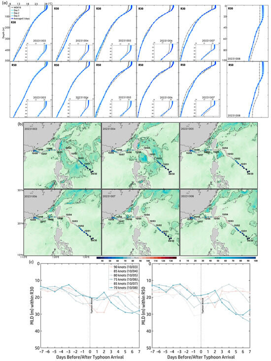
Figure 15.
(a) Three-day pre-temperature profiles within R30 and R50 along Typhoon Koinu (2023) from 3 October to 8 October. Light red curves represent daily temperature profiles, while red curves indicate the three-day averaged temperature profiles. Gray curves show the monthly temperature profiles from WOA18. (b) Daily MLD maps from 3 October to 8 October. (c) Time series of MLD ±7 days before and after Koinu’s arrival within R30 and R50. Colored curves correspond to the typhoon intensity scale.
The daily MLD maps (Figure 15b) depict the mixed layer evolution along Koinu’s track. On 3 October, when Koinu reached peak intensity (90 knots), MLD remained shallow (~30–40 m) in the WP, concentrating surface heat and supporting intensification. As Koinu moved westward into the SCS (4–5 October), MLD deepened slightly (~40–50 m) in localized regions due to typhoon-induced mixing. From 6 October to 8 October, as Koinu weakened, MLD gradually recovered, though it remained slightly deeper along the typhoon’s track, indicating persistent mixing effects. Figure 15c presents the time series of MLD within R30 (outer core) and R50 (near-inner core). Before Koinu’s arrival (Days −7 to −1): MLD remained stable (~25–30 m), reflecting minimal pre-typhoon disturbances. Upon arrival (Day 0): MLD deepened significantly, reaching ~35–40 m in R30 and ~30–35 m in R50, with greater deepening in R30, suggesting stronger mixing and upwelling effects in the outer-core region. Post-arrival (Days +1 to +7): MLD gradually returned to pre-typhoon levels by Day +7, reflecting the relaxation of typhoon-induced impacts. R30 exhibited greater MLD variability and deeper values than R50, indicating stronger wind stress and mixing effects in the outer core, while R50 retained more localized stratification. The MLD response to Typhoon Koinu highlights the dynamic nature of typhoon-induced ocean forcing. MLD deepened significantly during peak intensity, with more pronounced impacts in R30. Post-typhoon MLD recovery emphasizes the transient nature of these effects as subsurface processes gradually stabilize the upper ocean thermal structure. Variations between R30 and R50 reflect localized differences in mixing intensity, with stronger responses in the outer core compared to the inner core.
3.5. Air–Sea Heat Flux: Case Study
Heat flux variations in R30 (outer core) and R50 (near-inner core) under Typhoons Hinnamnor (2022), Mawar (2023), and Koinu (2023) reveal distinct yet interconnected air–sea exchange patterns, driven by typhoon intensity and oceanic conditions (Figure 16). For Hinnamnor (Figure 16a,b), total heat flux peaked at ~100 W/m2 on 31 August, aligning with its peak intensity (~100 knots). Latent heat flux (~120 W/m2) dominated the exchange, highlighting the role of evaporation. As Hinnamnor weakened, fluxes in R30 and R50 steadily declined (~60 W/m2), mirroring its dissipation phase. During its second intensification (4 September), fluxes remained lower, indicating weaker energy exchanges. R50 exhibited consistently higher fluxes than R30, reflecting stronger air–sea interactions near the inner core. For Mawar (Figure 16c,d), heat fluxes peaked at ~120 W/m2 on 26 May, coinciding with its peak intensity (115 knots). Fluxes in R50 were slightly higher than in R30, suggesting stronger air–sea coupling near the inner core. As Mawar weakened (27–30 May), heat fluxes steadily declined, mirroring reduced energy transfer and ocean–atmosphere interactions. For Koinu (Figure 16e,f), heat flux exhibited a more gradual decline (3–6 October), paralleling its weakening (65 to 35 W/m2). With a lower peak intensity (~90 knots) than Hinnamnor and Mawar, Koinu’s heat flux magnitudes were weaker. From 6 to 8 October, as Koinu re-intensified over the SCS, total heat flux increased slightly (~40 W/m2) before declining as the typhoon dissipated. These findings highlight latent heat flux as the dominant driver of air–sea exchange, with R50 consistently exhibiting stronger fluxes than R30. The variability in heat flux patterns underscores the dynamic nature of air–sea coupling across different ocean basins.
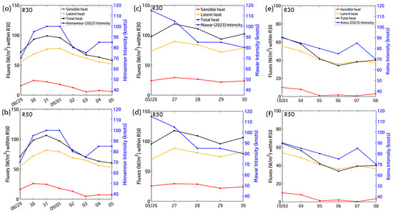
Figure 16.
Air–sea heat fluxes along the typhoon tracks within R30 and R50. (a,b) Hinnamnor (2022), (c,d) Mawar (2023), and (e,f) Koinu (2023). Total heat flux represents the sum of sensible and latent heat fluxes.
Across all three typhoons, latent heat flux dominated air–sea energy exchange, reinforcing its critical role in sustaining typhoon intensity, while sensible heat flux remained negligible. The total heat flux followed typhoon intensity trends, peaking during intensification and declining as typhoons weakened. In Hinnamnor and Mawar, R50 consistently exhibited stronger heat fluxes than R30, reflecting localized energy exchanges in the inner core. Koinu, however, showed less pronounced differences between R30 and R50, indicating more uniform air–sea interactions. These findings emphasize the importance of inner- and outer-core dynamics in modulating typhoon intensity and energy transfer. While latent heat flux drives ocean–atmosphere coupling, its magnitude varies across storms, depending on typhoon intensity, oceanic conditions, and spatial variability in heat exchange. The distinct responses in R30 and R50 highlight localized and large-scale processes in typhoon evolution, providing crucial insights into air–sea interactions and typhoon dissipation mechanisms.
4. Discussion
MHWs influence typhoon intensity by acting as an energy source and a disruptor. This study examines their dual role in Typhoons Hinnamnor (2022), Mawar (2023), and Koinu (2023) over the WP, ECS, and SCS. Before peak intensity, MHWs enhanced typhoon growth by providing heat through strong stratification. However, as typhoons progress, wind-driven mixing, and upwelling disrupt MHWs, depleting surface heat and accelerating intensity decay. This highlights MHWs’ contrasting effects, amplifying typhoons initially but later weakening them through oceanic heat loss. The findings underscore the importance of air–sea heat exchange and stratification variability in typhoon evolution.
4.1. Feedback Mechanism Between MHWs and Subsurface Ocean Conditions
Before the typhoon’s arrival, MHWs were driven by abnormally high SSTs, accompanied by the shoaling of the MLD and upper thermal structure (Figure 9, Figure 10, Figure 11, Figure 12, Figure 13, Figure 14 and Figure 15). The shallow MLD was linked to reduced wind-driven mixing, enhancing thermal stratification (Figure 13, Figure 14 and Figure 15). In 2022, MHW characteristics varied spatially, with lower frequency over the open ocean but prolonged durations along the Kuroshio Current, a key heat reservoir. Maximum intensities exceeding 3 °C were concentrated in the northern WP, particularly the ECS (Figure 5a–c), aligning with Typhoon Hinnamnor’s intensification phases.
Hinnamnor interacted with moderate MHW conditions (Category 1) across three domains, exhibiting distinct thermal dynamics. During its first intensification (29 August–31, Domain A), Hinnamnor strengthened over high-intensity MHW regions, with strong SST anomalies (Figure 5c and Figure 6a). Moving into Domain B (31 August–3 September), weakening coincided with declining MHW intensity (Figure 5c and Figure 6b). However, upon entering Domain C (ECS), MHW intensities exceeding 3 °C fueled re-intensification (Figure 5c and Figure 6c). Daily MHW variations seven days before and after Hinnamnor’s arrival showed a significant decline, correlating with typhoon-induced heat loss within R30 and R50 (Figure 7a and Figure 8a,b). The upper ocean thermal structure further confirms MHW-typhoon interactions. OHC remained elevated in R30, with a slight decrease in R50 post-typhoon, showing a clear link between typhoon intensity peaks and OHC reduction (Figure 9a and Figure 10a,b). Similarly, remained above 26.5 °C before and after passage, reinforcing its role in sustaining the MHW (Figure 11a and Figure 12a,b). Pre-typhoon stratification was strong, with MLDs of 10–20 m, but vertical mixing deepened MLDs to ~40 m within 1–3 days, leading to MHW dissipation (Figure 13). These findings highlight the interplay between subsurface heat reservoirs (OHC and ) and stratification in modulating typhoon intensity. The ECS provided an optimal environment for re-intensification, where MHWs and OHC synergistically fueled Hinnamnor’s first intensification, while MHWs played a dominant role in the second phase due to depth limitations on OHC. Intense vertical mixing eventually disrupted stratification, delaying MHW recovery. This study confirms that MHWs supply excess energy that would not be available under normal conditions [21,23,24]. Additionally, southerly winds linked to a delayed summer monsoon in 2022 prolonged MHWs, aligning with increased September MHW frequency [38]. This extended summer period, driven by global warming and anthropogenic influences, underscores the compounding effects of climate change on MHW occurrence and intensity [39].
In 2023, MHW frequency, duration, and intensity exhibited distinct spatial variability, with higher MHW frequency in the open ocean of the WP and the shallow waters of the SCS. These regions also experienced prolonged MHWs, with maximum intensities increasing from 0.5 °C in the open ocean to 2.5 °C in the SCS (Figure 5d–f). Typhoon Mawar (2023) formed over deeper waters, intensifying over regions where MHWs peaked at ~1 °C. As it moved westward, it encountered even stronger MHW conditions, yet its intensity declined on 27 May, eventually dissipating. This weakening coincided with a rapid decrease in MHW intensity, transitioning from strong MHW conditions to an absence of MHWs by 28 May (Figure 6d). Daily MHW variations seven days before and after Mawar’s arrival showed significant declines, mirroring reductions in typhoon intensity and OHC within R30 and R50 (Figure 7b and Figure 8c,d). From 26 May to 30 May, high OHC and values were observed, sustaining warm ocean conditions before and after Mawar’s passage. However, as Mawar weakened, OHC declined, particularly at higher latitudes (Figure 9b and Figure 10c,d). Despite this, subsurface temperatures remained warm, exceeding 27 °C in R30 and 26 °C in R50, indicating persistent thermal support despite surface cooling (Figure 11b and Figure 12c,d). Strong stratification along Mawar’s track contributed to its evolution, with MLD deepening rapidly to 35–45 m within R30 and R50 after passage (Figure 14). These findings highlight the key role of subsurface thermal conditions (OHC, , and stratification) in modulating Mawar’s intensification and dissipation. While MHWs contributed to favorable conditions for intensification, they could not fully control Mawar’s evolution. The persistence of MHWs in the NWP open ocean has been linked to anomalous ocean heat advection and reduced wind mixing [40]. Subsurface warming and weaker vertical mixing further intensified MHW conditions, prolonging their presence and strengthening their impact [41]. As global warming enhances upper ocean stratification [42], less effective detrainment from the mixed layer may limit subsurface heat storage, amplifying surface warming and intensifying MHWs. This escalation in heat stress and stratification raises concerns over cumulative impacts on marine ecosystems and primary production, particularly in pelagic environments [43,44].
Typhoon Koinu (2023) developed under lower MHW frequency and shorter durations during its initial intensification. However, as it moved westward, its intensity decreased over eastern and southern Taiwan, coinciding with declining MHW intensity (Figure 5d–f). Koinu peaked on 3 October, followed by gradual weakening until 6 October, during which MHW conditions in Domain A declined from moderate to absent (Figure 6e). Upon reaching the shallow waters of the SCS, Koinu encountered higher MHW intensities, particularly in Domain B (6–8 October), where MHW conditions persisted in Categories 1–2 (Figure 6f). These warmer conditions supported Koinu’s secondary intensification. Daily MHW variations seven days before and after its arrival showed a consistent decrease in both MHW intensity and typhoon strength, along with reductions in OHC within R30 and R50, directly correlating with Koinu’s weakening (Figure 7c and Figure 8d,e). Surface MHWs and warm subsurface conditions drove Koinu’s initial intensification in the NWP. In the shallow SCS, despite lower OHC due to depth constraints, strong MHWs compensated for reduced heat storage, supporting re-intensification. Warm OHC conditions (>100 kJ/cm2) persisted within R30 and R50 before and after passage, though they were lower (~80 kJ/cm2) in the SCS due to bathymetric limitations (Figure 9c and Figure 10e,f). The remained between 27.5 °C and 29 °C, indicating a sustained subsurface heat reservoir (Figure 11c and Figure 12e,f). Strong stratification was observed along Koinu’s track, with MLDs of 10–30 m, which deepened slightly post-typhoon before recovering within two days (Figure 15). MHWs arise from a complex interplay of local and large-scale processes, influenced by oceanic–atmospheric dynamics and remote teleconnections [45]. Recent studies indicate that MHWs in the SCS exhibit strong interannual and interdecadal variability, closely tied to climate modes like ENSO [46]. Additional factors contributing to MHW persistence include weakened local upwelling, reduced entrainment processes, and Arctic amplification, which slows upper-level Rossby waves, increasing MHW occurrence [47,48]. These findings emphasize the complex, interconnected drivers behind MHWs, highlighting the importance of integrating regional and global perspectives for improved understanding and prediction.
Basin-specific thermal dynamics shape the dual effects of MHWs on typhoon intensification and dissipation. In the ECS and NWP, high OHC and provide a substantial heat reservoir, supporting typhoon intensification. However, deeper MLDs in these regions slow MHW recovery after typhoon-induced vertical mixing, as heat is redistributed across greater depths. In contrast, the SCS, with shallower bathymetry and lower OHC, facilitates faster MHW recovery. This allows the region to sustain favorable conditions for typhoon re-intensification, even after significant weakening. These findings highlight the complex feedback mechanisms between MHWs and subsurface ocean conditions, where OHC and play key roles in modulating both MHW persistence and typhoon dynamics. The interplay between MHWs and subsurface thermal structure underscores the importance of regional ocean conditions in shaping typhoon intensity and the subsequent dissipation or recovery of MHWs across different basins.
4.2. Feedback Mechanism Between MHWs and Air–Sea Heat Fluxes
The interaction between MHWs and air–sea heat fluxes plays a crucial role in modulating typhoon intensity and dissipation. Latent and sensible heat fluxes govern energy exchange between the ocean and atmosphere, directly influencing typhoon evolution. Throughout all three cases, latent heat flux dominated total heat exchange, reaching up to 120 W/m2 at peak intensity. The persistent role of evaporative processes in sustaining typhoon strength is evident, with R50 consistently exhibiting stronger fluxes than R30, reflecting enhanced energy transfer near the inner core. MHW-induced SST anomalies intensified latent heat fluxes by increasing evaporation rates, directly reinforcing typhoon intensity. During Hinnamnor and Mawar’s peak stages, warm surface conditions from MHWs elevated heat exchange in R50, strengthening the typhoons. As they weakened, heat fluxes declined, coinciding with reductions in MHW intensity and the disruption of air–sea coupling, particularly during their dissipation phases.
Basin-specific thermal characteristics further influence heat flux responses. In the WP and ECS, strong thermal stratification, elevated OHC, and concentrated heat fluxes near the inner core, promoting intensification but delaying post-typhoon recovery due to deep vertical mixing. In contrast, the SCS, with its shallower bathymetry and weaker stratification, exhibited more uniform heat flux distributions between R30 and R50, as observed during Koinu’s passage. Rapid MHW recovery in the SCS sustained moderate heat fluxes, facilitating localized re-intensification. These patterns emphasize the dominant role of latent heat flux in driving typhoon intensity while also highlighting spatial variability in air–sea coupling. Strong heat fluxes in R50 are critical for peak intensification, whereas broader flux distributions in R30 illustrate the extent of typhoon-ocean interactions.
Beyond oceanic influences, MHWs also modify atmospheric conditions that affect typhoon evolution. Elevated SST anomalies boost latent heat fluxes, increasing lower-level moisture and mid-level humidity to enhance deep convection and intensification. However, vertical wind shear can disrupt this process by modulating convection efficiency [14,24,49,50,51]. As climate change alters atmospheric moisture, wind shear, and upper-level temperatures, the interaction between MHWs and typhoon intensity becomes more complex. Although this study focuses on oceanic thermal anomalies, future research should integrate ocean–atmosphere coupling and basin-specific analyses—using frameworks like a multi-variable phase-space approach with VWS and OHC—to improve intensity predictions under changing climate conditions.
5. Conclusions
Based on an analysis of 1027 typhoon position cases from 1993 to 2023, the results indicate that while MHW intensity remains relatively high before typhoon arrival (Day −7 to Day 0), it exhibits a significant decline after typhoon passage, highlighting the disruptive impact of typhoons on MHW structures. This effect is particularly pronounced for stronger typhoons (e.g., Violent and Very Strong), which induce intense vertical mixing and upwelling, leading to the rapid dissipation of MHWs. In contrast, weaker typhoons also contribute to MHW reduction, albeit to a lesser extent. Regionally, semi-enclosed seas such as the SCS and ECS tend to accumulate higher heat levels, resulting in stronger MHWs; however, these regions also experience more severe MHW dissipation following typhoon passage. The WP exhibits a lower average MHW intensity but follows a similar dissipation trend. Moreover, no monotonic or linear relationship is observed between typhoon intensity rate and MHW category, suggesting a potential bidirectional interaction between the two. These findings collectively indicate that MHW persistence and dissipation are strongly influenced by typhoon intensity and interaction duration, emphasizing the critical role of typhoon-affected regions in modulating energy exchange processes.
This study examines the dual effects of MHWs on typhoon intensity and dissipation, analyzing case studies of Typhoons Hinnamnor (2022), Mawar (2023), and Koinu (2023) across the WP, ECS, and SCS. Moderate to strong MHWs along typhoon tracks provided substantial energy for intensification, driven by elevated SST, high OHC, and , supported by shallow MLD and strong stratification. However, MHWs dissipated post-typhoon due to intense vertical mixing, upwelling, and surface cooling, underscoring their role as energy reservoirs and transient features influenced by typhoon-induced processes. Elevated OHC and (>26.5 °C) concentrated near the surface in highly stratified regions, particularly in the ECS and WP, supported peak intensification phases of Hinnamnor and Mawar. Conversely, MHW dissipation was strongest in the ECS and WP, where typhoon-induced vertical mixing redistributed heat, depleting OHC and weakening stratification. These effects were most pronounced in R50, where post-typhoon heat loss slowed recovery. In contrast, the shallow bathymetry of the SCS allowed rapid MHW recovery, sustaining favorable conditions for Koinu’s secondary intensification. These findings emphasize the regional variability in MHW–typhoon interactions, shaped by basin-specific thermal dynamics. Latent heat flux emerged as the dominant driver of energy exchange, with higher fluxes in R50 than R30, highlighting the importance of inner-core dynamics in modulating typhoon evolution. Variability in heat fluxes further underscores the dynamic nature of air–sea coupling, influenced by regional stratification, OHC, and thermocline depths.
This study illustrates that MHWs and typhoons mutually interact, forming compound extreme events. MHWs can intensify typhoons, while typhoons can diminish MHWs, demonstrating a complex feedback mechanism between oceanic and atmospheric processes. These findings provide critical insights into compound extreme events and their implications for marine ecosystems and atmospheric dynamics. Under future warming scenarios, both MHWs and typhoons are projected to increase in frequency and intensity [9,45,52], amplifying the co-occurrence of extreme events and posing greater risks to coastal and marine systems. Understanding these interactions is crucial for assessing climate change impacts on marine ecosystems and coastal populations, as well as for improving predictions of MHW intensity variations across different regions.
Author Contributions
Conceptualization, T.-K.-D.N. and P.-C.H.; methodology, T.-K.-D.N. and P.-C.H.; software, T.-K.-D.N. and P.-C.H.; validation, P.-C.H.; formal analysis, T.-K.-D.N. and P.-C.H.; investigation, T.-K.-D.N.; resources, P.-C.H.; data curation, T.-K.-D.N.; writing—original draft preparation, T.-K.-D.N. and P.-C.H.; writing—review and editing, P.-C.H.; visualization, T.-K.-D.N. and P.-C.H.; supervision, P.-C.H.; project administration, P.-C.H.; funding acquisition, P.-C.H. All authors have read and agreed to the published version of the manuscript.
Funding
This research was funded by the National Science and Technology Council, grant number 112-2621-M-008-002 and the APC was funded by 113-2611-M-008-003.
Data Availability Statement
The information on typhoon data are provided by the Japan Meteorological Agency (JMA, https://www.jma.go.jp/ (accessed on 25 December 2024)); The reanalysis dataset is provided by E.U. Copernicus Marine Service Information (https://doi.org/10.48670/moi-00021 (accessed on 25 December 2024)); The WOA18 climatology dataset is provided by NOAA National Centers for Environmental Information (https://www.ncei.noaa.gov/access/world-ocean-atlas-2018/ (accessed on 25 December 2024)); The ECMWF heat fluxes dataset is provided by Copernicus Climate Data Store (https://cds.climate.copernicus.eu/ (accessed on 25 December 2024)).
Acknowledgments
The authors acknowledge and appreciate the availability of all data used in this study, obtained from open-access databases. The authors thank anonymous reviewers and academic editors for their comments.
Conflicts of Interest
The authors declare no conflicts of interest.
Abbreviations
The following abbreviations are used in this manuscript:
| CMEMS | Copernicus Marine Environment Monitoring Service |
| D26 | Depth of the 26 °C isotherm |
| ENSO | El Niño-Southern Oscillation |
| ECS | East China Sea |
| ECMWF | European Centre for Medium-Range Weather Forecasts |
| JMA | Japan Meteorological Agency |
| MHWs | Marine heatwaves |
| MLD | Mixed layer depth |
| NCEI | National Centers for Environmental Information |
| NOAA | National Oceanic and Atmospheric Administration |
| NWP | Northwestern Pacific |
| OHC | Ocean heat content |
| PDO | Pacific Decadal Oscillation |
| R30 | Outer-core region (radii of 30 knots) |
| R50 | Inner-core region (radii of 50 knots) |
| SCS | South China Sea |
| SST | Sea surface temperature |
| Mean upper 100 m temperature | |
| WOA18 | World Ocean Atlas 2018 |
References
- Hobday, A.J.; Alexander, L.V.; Perkins, S.E.; Smale, D.A.; Straub, S.C.; Oliver, E.C.; Benthuysen, J.A.; Burrows, M.T.; Donat, M.G.; Feng, M.; et al. A hierarchical approach to defining marine heatwaves. Prog. Oceanogr. 2016, 141, 227–238. [Google Scholar] [CrossRef]
- Oliver, E.C.; Donat, M.G.; Burrows, M.T.; Moore, P.J.; Smale, D.A.; Alexander, L.V.; Benthuysen, J.A.; Feng, M.; Gupta, A.S.; Hobday, A.J.; et al. Longer and more frequent marine heatwaves over the past century. Nat. Commun. 2018, 9, 1324. [Google Scholar] [CrossRef]
- Sen Gupta, A.; Thomsen, M.; Benthuysen, J.A.; Hobday, A.J.; Oliver, E.; Alexander, L.V.; Burrows, M.T.; Donat, M.G.; Feng, M.; Holbrook, N.J.; et al. Drivers and impacts of the most extreme marine heatwave events. Sci. Rep. 2020, 10, 19359. [Google Scholar] [CrossRef]
- Hsu, P.C.; Macagga, R.A.T.; Lu, C.Y.; Lo, D.Y.J. Investigation of the Kuroshio-coastal current interaction and marine heatwave trends in the coral habitats of Northeastern Taiwan. Reg. Stud. Mar. Sci. 2024, 71, 103431. [Google Scholar] [CrossRef]
- Hsu, P.C.; Macagga, R.A.T.; Raj, R.P. Assessment of the impacts of rapid Marine Heatwaves and cumulative thermal stress on cold-water upwelling coral refugia. Geomat. Nat. Hazards Risk 2025, 16, 2448240. [Google Scholar] [CrossRef]
- Holbrook, N.J.; Scannell, H.A.; Sen Gupta, A.; Benthuysen, J.A.; Feng, M.; Oliver, E.C.; Alexander, L.V.; Burrows, M.T.; Donat, M.G.; Hobday, A.J.; et al. A global assessment of marine heatwaves and their drivers. Nat. Commun. 2019, 10, 2624. [Google Scholar] [CrossRef]
- Myers, T.A.; Mechoso, C.R.; Cesana, G.V.; DeFlorio, M.J.; Waliser, D.E. Cloud feedback key to marine heatwave off Baja California. Geophys. Res. Lett. 2018, 45, 4345–4352. [Google Scholar] [CrossRef]
- Chen, Q.; Li, D.; Feng, J.; Zhao, L.; Qi, J.; Yin, B. Understanding the compound marine heatwave and low-chlorophyll extremes in the western Pacific Ocean. Front. Mar. Sci. 2023, 10, 1303663. [Google Scholar] [CrossRef]
- Frölicher, T.L.; Fischer, E.M.; Gruber, N. Marine heatwaves under global warming. Nature 2018, 560, 360–364. [Google Scholar] [CrossRef]
- Song, Q.; Yao, Y.; Wang, C. Response of future summer marine heatwaves in the South China Sea to enhanced western Pacific subtropical high. Geophys. Res. Lett. 2023, 50, e2023GL103667. [Google Scholar] [CrossRef]
- Yang, Y.; Sun, W.; Yang, J.; Lim Kam Sian, K.T.; Ji, J.; Dong, C. Analysis and prediction of marine heatwaves in the Western North Pacific and Chinese coastal region. Front. Mar. Sci. 2022, 9, 1048557. [Google Scholar] [CrossRef]
- Xu, J.; Yan, Y.; Zhang, L.; Xing, W.; Meng, L.; Yu, Y.; Chen, C. Long-term trends and extreme events of marine heatwaves in the Eastern China Marginal Seas during summer. Front. Mar. Sci. 2024, 11, 1380963. [Google Scholar] [CrossRef]
- Emanuel, K. Tropical cyclones. Annu. Rev. Earth Planet. Sci. 2003, 31, 75–104. [Google Scholar] [CrossRef]
- Cione, J.J. The relative roles of the ocean and atmosphere as revealed by buoy air–sea observations in hurricanes. Mon. Weather Rev. 2015, 143, 904–913. [Google Scholar] [CrossRef]
- Cione, J.J.; Uhlhorn, E.W. Sea surface temperature variability in hurricanes: Implications with respect to intensity change. Mon. Weather Rev. 2003, 131, 1783–1796. [Google Scholar] [CrossRef]
- Huang, P.; Lin, I.I.; Chou, C.; Huang, R.H. Change in ocean subsurface environment to suppress tropical cyclone intensification under global warming. Nat. Commun. 2015, 6, 7188. [Google Scholar] [CrossRef] [PubMed]
- Lin, I.I.; Pun, I.F.; Lien, C.C. “Category-6” supertyphoon Haiyan in global warming hiatus: Contribution from subsurface ocean warming. Geophys. Res. Lett. 2014, 41, 8547–8553. [Google Scholar] [CrossRef]
- Kataoka, T.; Tozuka, T.; Yamagata, T. Generation and decay mechanisms of Ningaloo Niño/Niña. J. Geophys. Res. Ocean. 2017, 122, 8913–8932. [Google Scholar] [CrossRef]
- Dzwonkowski, B.; Coogan, J.; Fournier, S.; Lockridge, G.; Park, K.; Lee, T. Compounding impact of severe weather events fuels marine heatwave in the coastal ocean. Nat. Commun. 2020, 11, 4623. [Google Scholar] [CrossRef]
- Oh, H.; Kim, G.U.; Chu, J.E.; Lee, K.; Jeong, J.Y. The record-breaking 2022 long-lasting marine heatwaves in the East China Sea. Environ. Res. Lett. 2023, 18, 064015. [Google Scholar] [CrossRef]
- Choi, H.Y.; Park, M.S.; Kim, H.S.; Lee, S. Marine heatwave events strengthen the intensity of tropical cyclones. Commun. Earth Environ. 2024, 5, 69. [Google Scholar] [CrossRef]
- Gao, G.; Marin, M.; Feng, M.; Yin, B.; Yang, D.; Feng, X.; Ding, Y.; Song, D. Drivers of marine heatwaves in the East China Sea and the South Yellow Sea in three consecutive summers during 2016–2018. J. Geophys. Res. Ocean. 2020, 125, e2020JC016518. [Google Scholar] [CrossRef]
- Pun, I.F.; Hsu, H.H.; Moon, I.J.; Lin, I.I.; Jeong, J.Y. Marine heatwave as a supercharger for the strongest typhoon in the East China Sea. npj Clim. Atmos. Sci. 2023, 6, 128. [Google Scholar] [CrossRef]
- Rathore, S.; Goyal, R.; Jangir, B.; Ummenhofer, C.C.; Feng, M.; Mishra, M. Interactions between a marine heatwave and Tropical Cyclone Amphan in the Bay of Bengal in 2020. Front. Clim. 2022, 4, 861477. [Google Scholar] [CrossRef]
- Lee, S.; Park, M.S.; Kwon, M.; Park, Y.G.; Kim, Y.H.; Choi, N. Rapidly changing East Asian marine heatwaves under a warming climate. J. Geophys. Res. Ocean. 2023, 128, e2023JC019761. [Google Scholar] [CrossRef]
- Yao, Y.; Wang, C. Variations in summer marine heatwaves in the South China Sea. J. Geophys. Res. Ocean. 2021, 126, e2021JC017792. [Google Scholar] [CrossRef]
- Tan, H.J.; Cai, R.S.; Wu, R.G. Summer marine heatwaves in the South China Sea: Trend, variability and possible causes. Adv. Clim. Change Res. 2022, 13, 323–332. [Google Scholar] [CrossRef]
- Yao, Y.; Wang, C.; Wang, C. Record-breaking 2020 summer marine heatwaves in the western North Pacific. Deep Sea Res. Part II Top. Stud. Oceanogr. 2023, 209, 105288. [Google Scholar] [CrossRef]
- Han, T.; Xu, K.; Wang, L.; Liu, B.; Tam, C.Y.; Liu, K.; Wang, W. Extremely long-lived marine heatwave in South China Sea during summer 2020: Combined effects of the seasonal and intraseasonal variations. Glob. Planet. Change 2023, 230, 104261. [Google Scholar] [CrossRef]
- Hobday, A.J.; Oliver, E.C.J.; Gupta, A.S.; Benthuysen, J.A.; Burrows, M.T.; Donat, M.G.; Holbrook, N.J.; Moore, P.J.; Thomsen, M.S.; Wernberg, T.; et al. Categorizing and naming marine heatwaves. Oceanography 2018, 31, 162–173. Available online: https://www.jstor.org/stable/26542662 (accessed on 25 December 2024). [CrossRef]
- Taburet, G.; Sanchez-Roman, A.; Ballarotta, M.; Pujol, M.-I.; Legeais, J.-F.; Fournier, F.; Faugere, Y.; Dibarboure, G. DUACS DT2018: 25 years of reprocessed sea level altimetry products. Ocean Sci. 2019, 15, 1207–1224. [Google Scholar] [CrossRef]
- Artana, C.; Ferrari, R.; Bricaud, C.; Lellouche, J.-M.; Garric, G.; Sennéchael, N.; Lee, J.-H.; Park, Y.-H.; Provost, C. Twenty-five years of Mercator ocean reanalysis GLORYS12 at Drake Passage: Velocity assessment and total volume transport. Adv. Space Res. 2021, 68, 447–466. [Google Scholar] [CrossRef]
- Jean-Michel, L.; Eric, G.; Romain, B.-B.; Gilles, G.; Angélique, M.; Marie, D.; Clément, B.; Mathieu, H.; Olivier, L.G.; Charly, R.; et al. The Copernicus global 1/12 oceanic and sea ice GLORYS12 reanalysis. Front. Earth Sci. 2021, 9, 698876. [Google Scholar] [CrossRef]
- Locarnini, M.M.; Mishonov, A.V.; Baranova, O.K.; Boyer, T.P.; Zweng, M.M.; Garcia, H.E.; Reagan, J.; Seidov, D.; Weathers, K.W.; Paver, C.R.; et al. World Ocean Atlas 2018, Volume 1: Temperature. 2018, Ref. NOAA Atlas NESDIS 81, 52p. A. Mishonov Technical Editor. Available online: https://archimer.ifremer.fr/doc/00651/76338/ (accessed on 25 December 2024).
- Cucchi, M.; Weedon, G.P.; Amici, A.; Bellouin, N.; Lange, S.; Schmied, H.M.; Hersbach, H.; Buontempo, C. WFDE5: Bias-adjusted ERA5 reanalysis data for impact studies. Earth Syst. Sci. Data 2020, 12, 2097–2120. [Google Scholar] [CrossRef]
- Hersbach, H.; Bell, B.; Berrisford, P.; Hirahara, S.; Horányi, A.; Muñoz-Sabater, J.; Nicolas, J.; Peubey, C.; Radu, R.; Schepers, D.; et al. The ERA5 global reanalysis. Q. J. R. Meteorol. Soc. 2020, 146, 1999–2049. [Google Scholar] [CrossRef]
- Hsu, P.C.; Ho, C.R. Typhoon-induced ocean subsurface variations from glider data in the Kuroshio region adjacent to Taiwan. J. Oceanogr. 2019, 75, 1–21. [Google Scholar] [CrossRef]
- Ha, K.J.; Moon, S.; Timmermann, A.; Kim, D. Future changes of summer monsoon characteristics and evaporative demand over Asia in CMIP6 simulations. Geophys. Res. Lett. 2020, 47, e2020GL087492. [Google Scholar] [CrossRef]
- Moon, S.; Ha, K.J. Future changes in monsoon duration and precipitation using CMIP6. npj Clim. Atmos. Sci. 2020, 3, 45. [Google Scholar] [CrossRef]
- Benthuysen, J.A.; Smith, G.A.; Spillman, C.M.; Steinberg, C.R. Subseasonal prediction of the 2020 Great Barrier Reef and Coral Sea marine heatwave. Environ. Res. Lett. 2021, 16, 124050. [Google Scholar] [CrossRef]
- Scannell, H.A.; Johnson, G.C.; Thompson, L.; Lyman, J.M.; Riser, S.C. Subsurface evolution and persistence of marine heatwaves in the Northeast Pacific. Geophys. Res. Lett. 2020, 47, e2020GL090548. [Google Scholar] [CrossRef]
- Li, G.; Cheng, L.; Zhu, J.; Trenberth, K.E.; Mann, M.E.; Abraham, J.P. Increasing ocean stratification over the past half-century. Nat. Clim. Change 2020, 10, 1116–1123. [Google Scholar] [CrossRef]
- Jacox, M.G.; Hazen, E.L.; Zaba, K.D.; Rudnick, D.L.; Edwards, C.A.; Moore, A.M.; Bograd, S.J. Impacts of the 2015–2016 El Niño on the California Current System: Early assessment and comparison to past events. Geophys. Res. Lett. 2016, 43, 7072–7080. [Google Scholar] [CrossRef]
- Smale, D.A.; Wernberg, T.; Oliver, E.C.J.; Thomsen, M.; Harvey, B.P.; Straub, S.C.; Burrows, M.T.; Alexander, L.V.; Benthuysen, J.A.; Donat, M.G.; et al. Marine heatwaves threaten global biodiversity and the provision of ecosystem services. Nat. Clim. Change 2019, 9, 306–312. [Google Scholar] [CrossRef]
- Holbrook, N.J.; Gupta, A.S.; Oliver, E.C.J.; Hobday, A.J.; Benthuysen, J.A.; Scannell, H.A.; Smale, D.A.; Wernberg, T. Keeping pace with marine heatwaves. Nat. Rev. Earth Environ. 2020, 1, 482–493. [Google Scholar] [CrossRef]
- Liu, K.; Xu, K.; Zhu, C.; Liu, B. Diversity of marine heatwaves in the South China Sea regulated by ENSO phase. J. Clim. 2022, 35, 877–893. [Google Scholar] [CrossRef]
- Oliver, E.C.; Benthuysen, J.A.; Bindoff, N.L.; Hobday, A.J.; Holbrook, N.J.; Mundy, C.N.; Perkins-Kirkpatrick, S.E. The unprecedented 2015/16 Tasman Sea marine heatwave. Nat. Commun. 2017, 8, 16101. [Google Scholar] [CrossRef]
- Benthuysen, J.A.; Oliver, E.C.; Feng, M.; Marshall, A.G. Extreme marine warming across tropical Australia during austral summer 2015–2016. J. Geophys. Res. Ocean. 2018, 123, 1301–1326. [Google Scholar] [CrossRef]
- Fritz, C.; Wang, Z. Water vapor budget in a developing tropical cyclone and its implication for tropical cyclone formation. J. Atmos. Sci. 2014, 71, 4321–4332. [Google Scholar] [CrossRef]
- Park, M.S.; Elsberry, R.L. Latent heating and cooling rates in developing and nondeveloping tropical disturbances during TCS-08: TRMM PR versus ELDORA retrievals. J. Atmos. Sci. 2013, 70, 15–35. [Google Scholar] [CrossRef]
- Park, M.S.; Elsberry, R.L.; Harr, P.A. Vertical wind shear and ocean heat content as environmental modulators of western North Pacific tropical cyclone intensification and decay. Trop. Cyclone Res. Rev. 2012, 1, 448–457. [Google Scholar] [CrossRef]
- Knutson, T.R.; Sirutis, J.J.; Zhao, M.; Tuleya, R.E.; Bender, M.; Vecchi, G.A.; Villarini, G.; Chavas, D. Global projections of intense tropical cyclone activity for the late twenty-first century from dynamical downscaling of CMIP5/RCP4. 5 scenarios. J. Clim. 2015, 28, 7203–7224. [Google Scholar] [CrossRef]
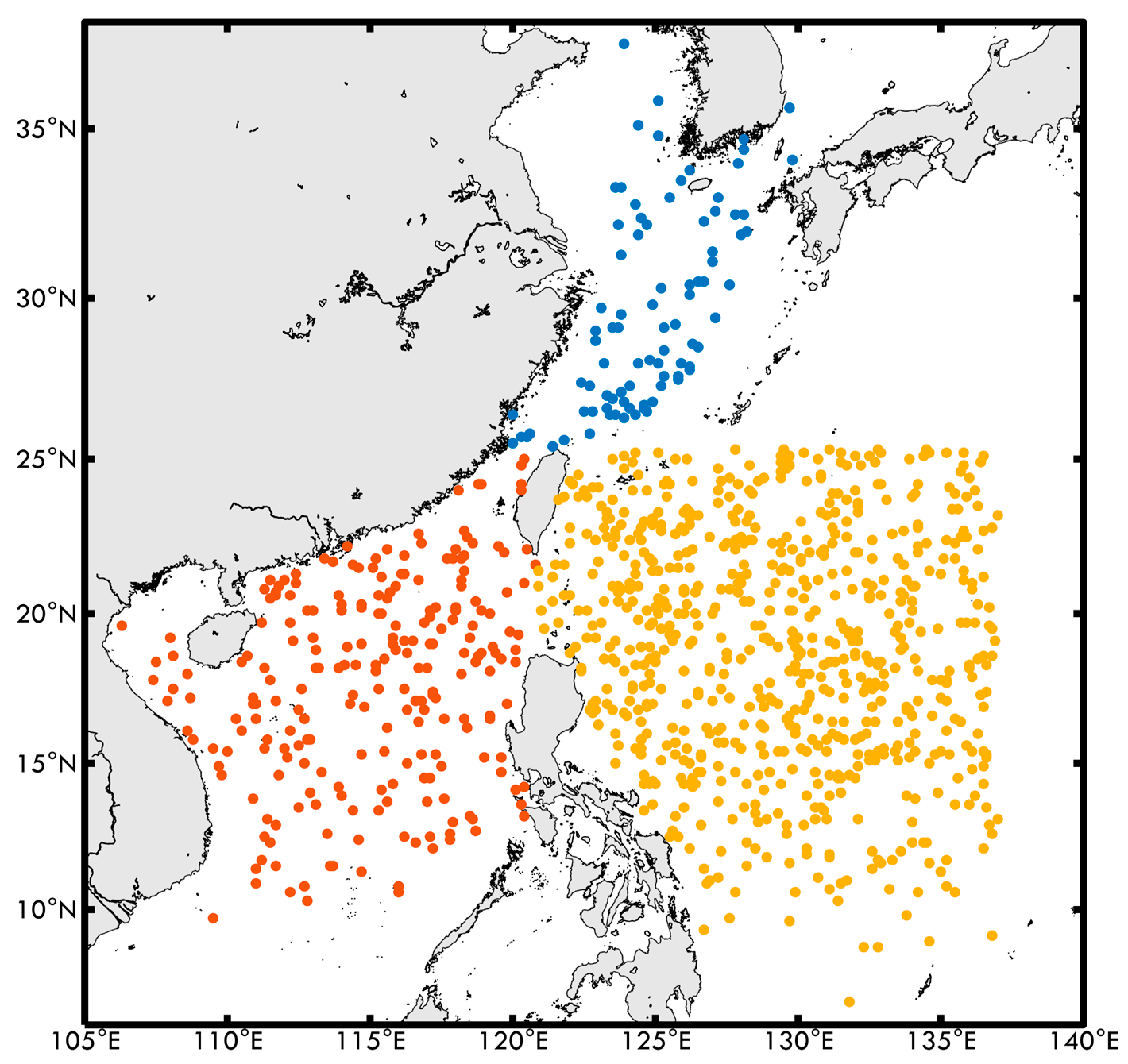
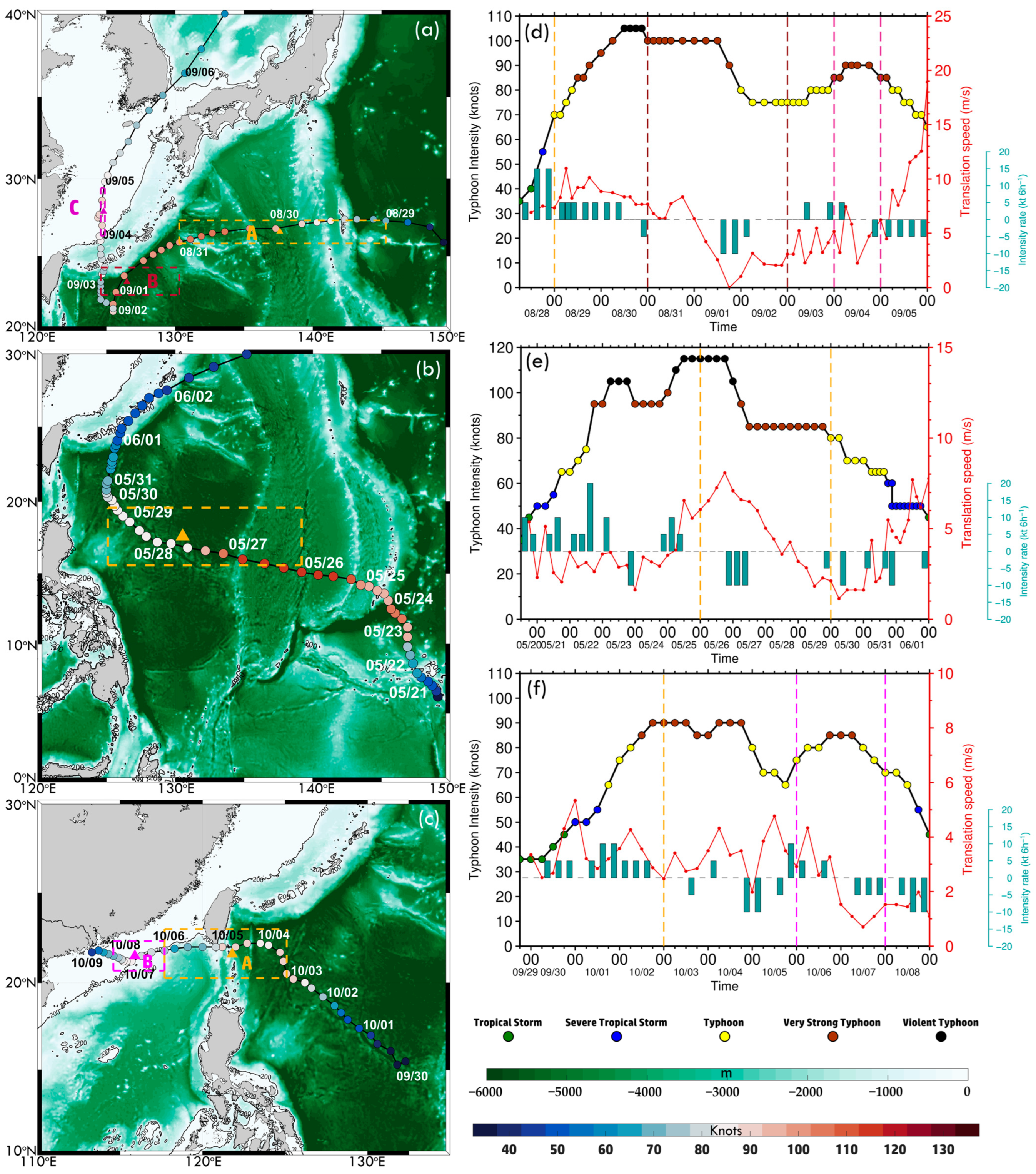
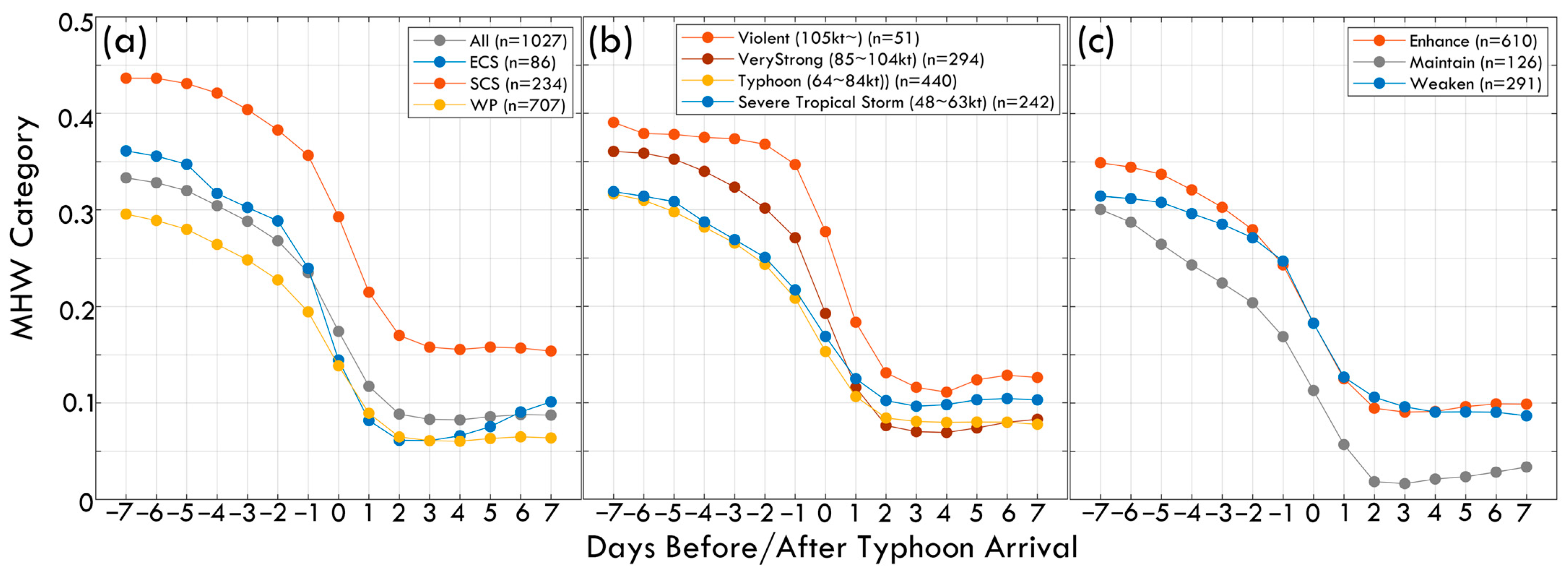
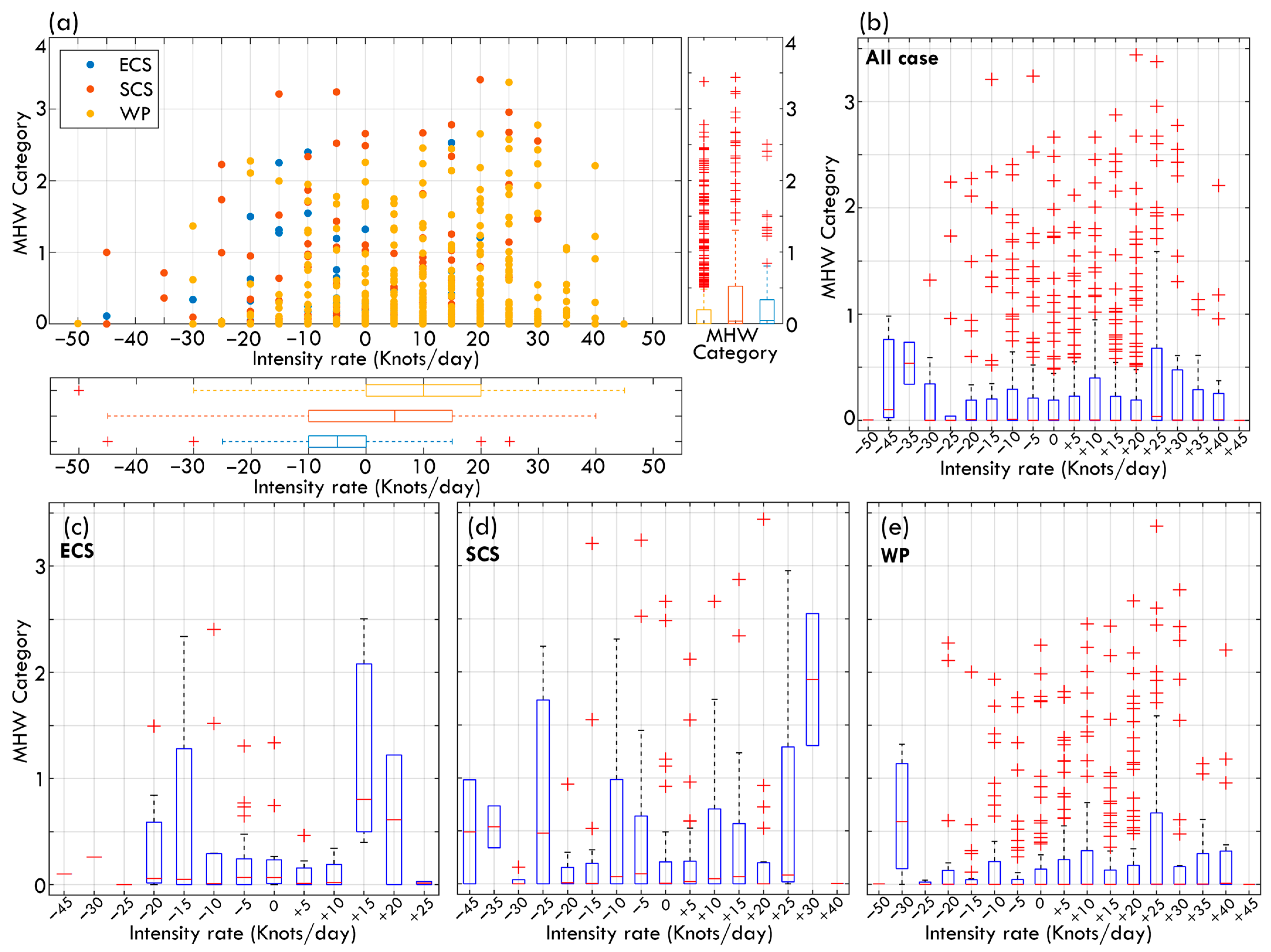
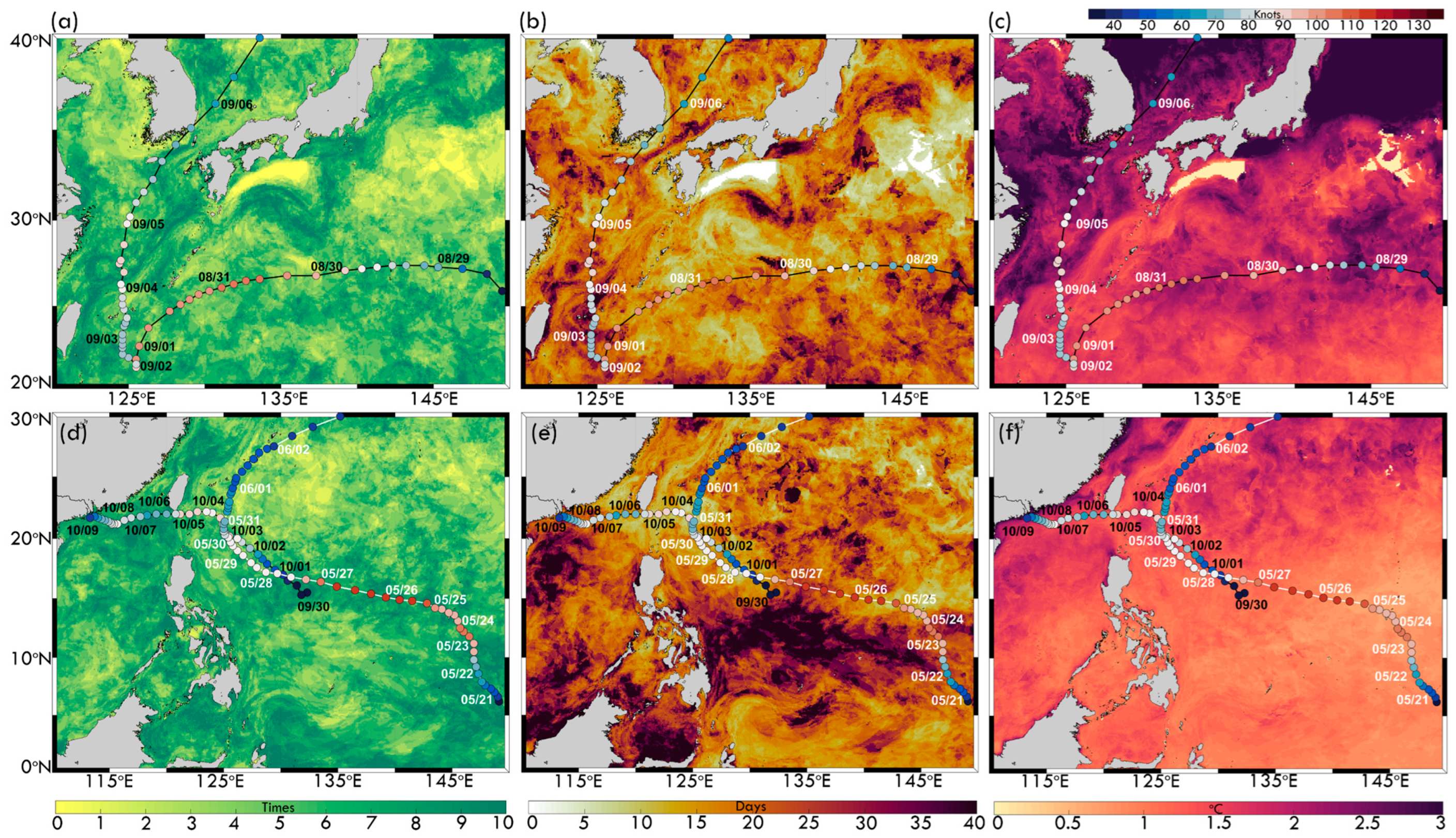
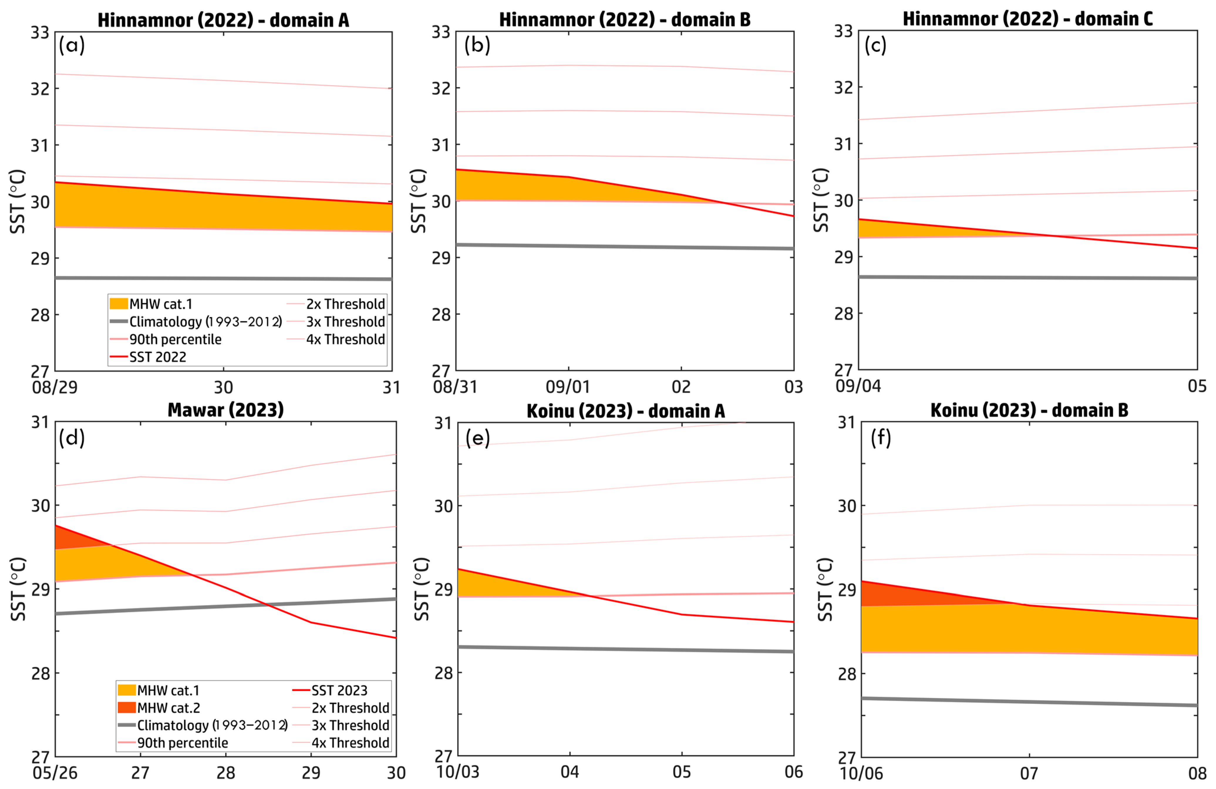
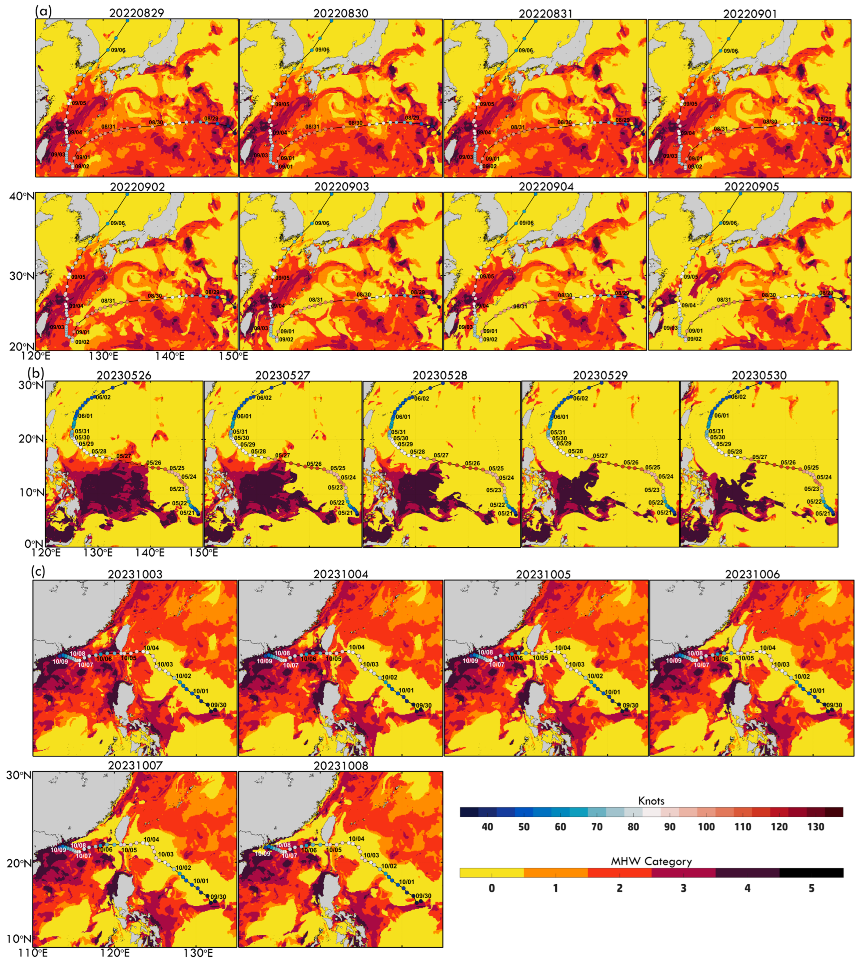
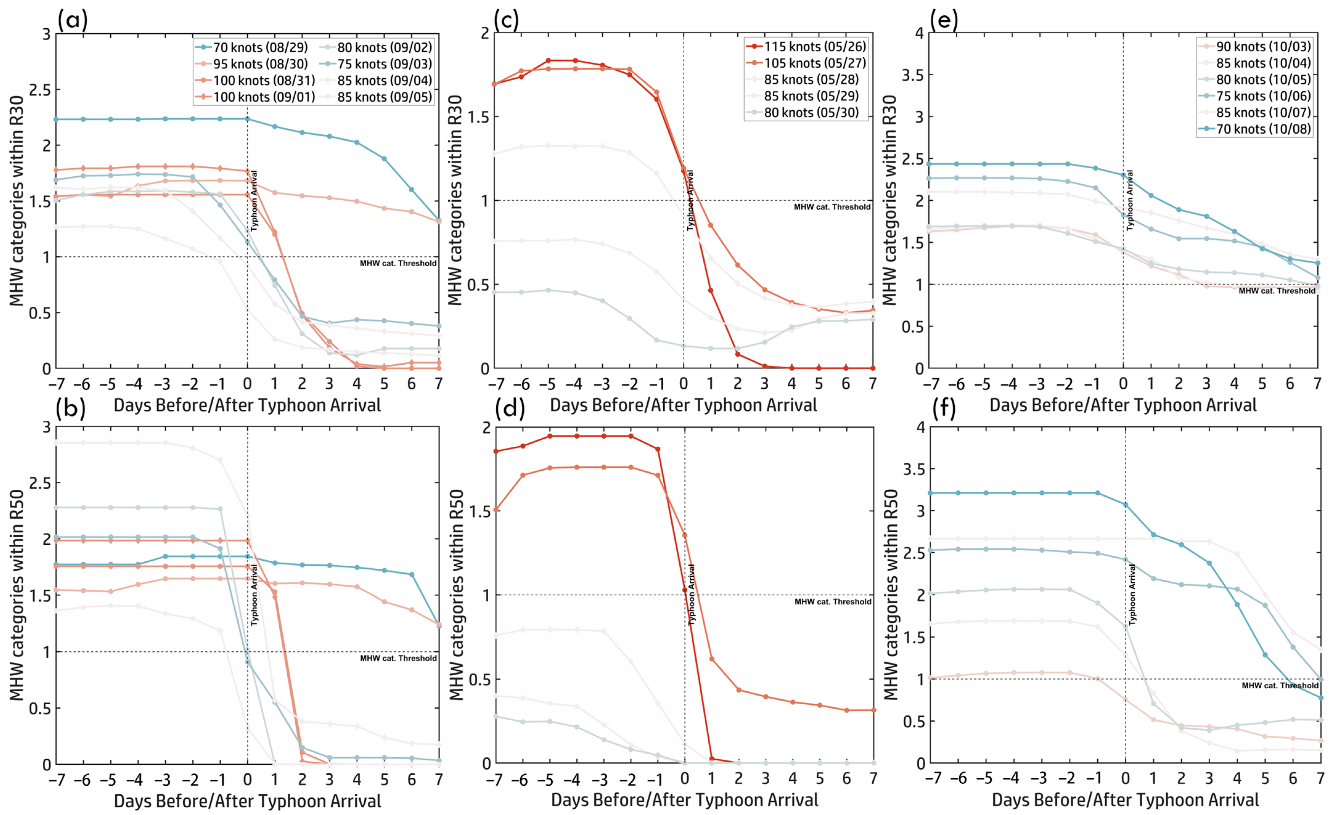
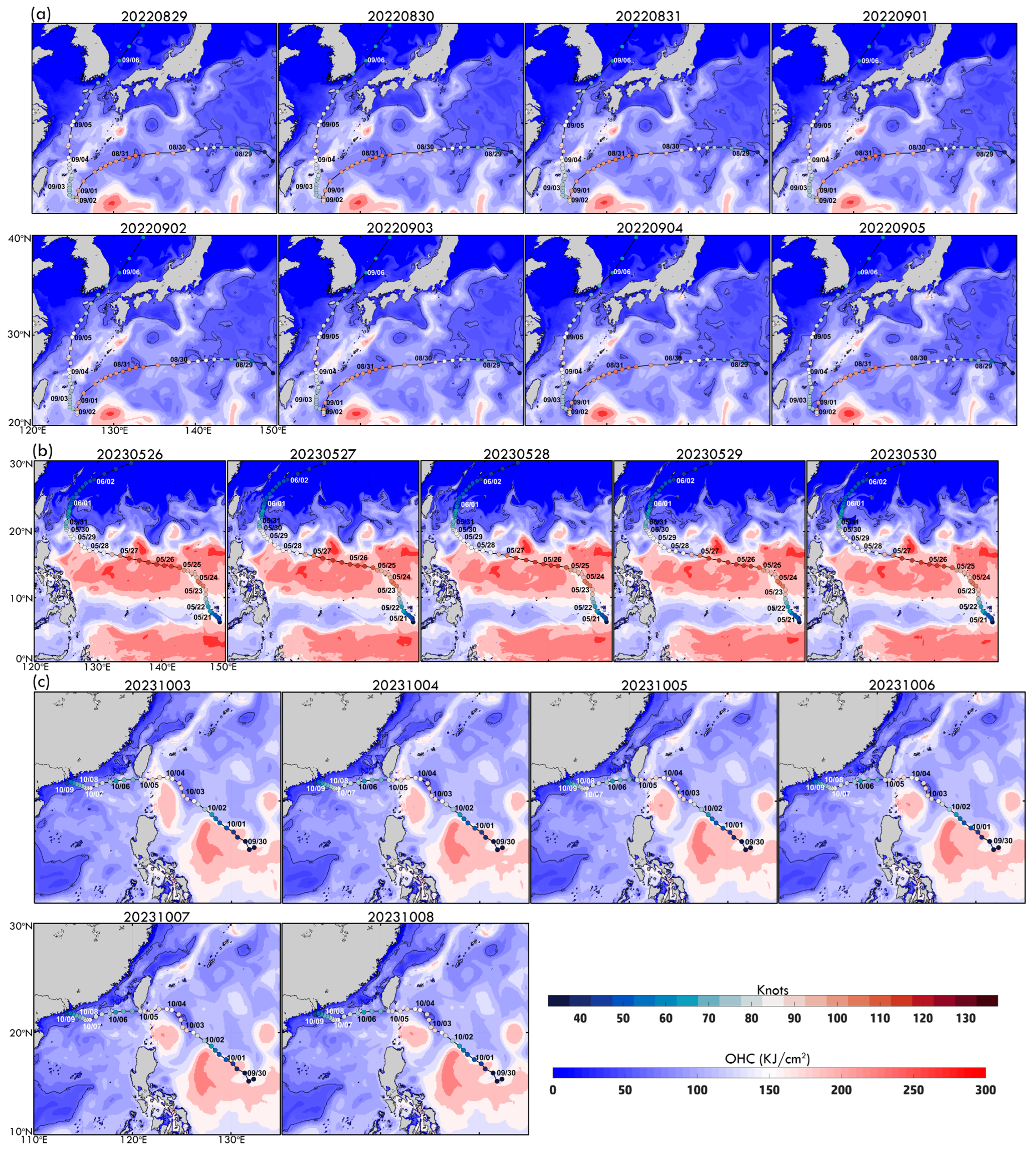
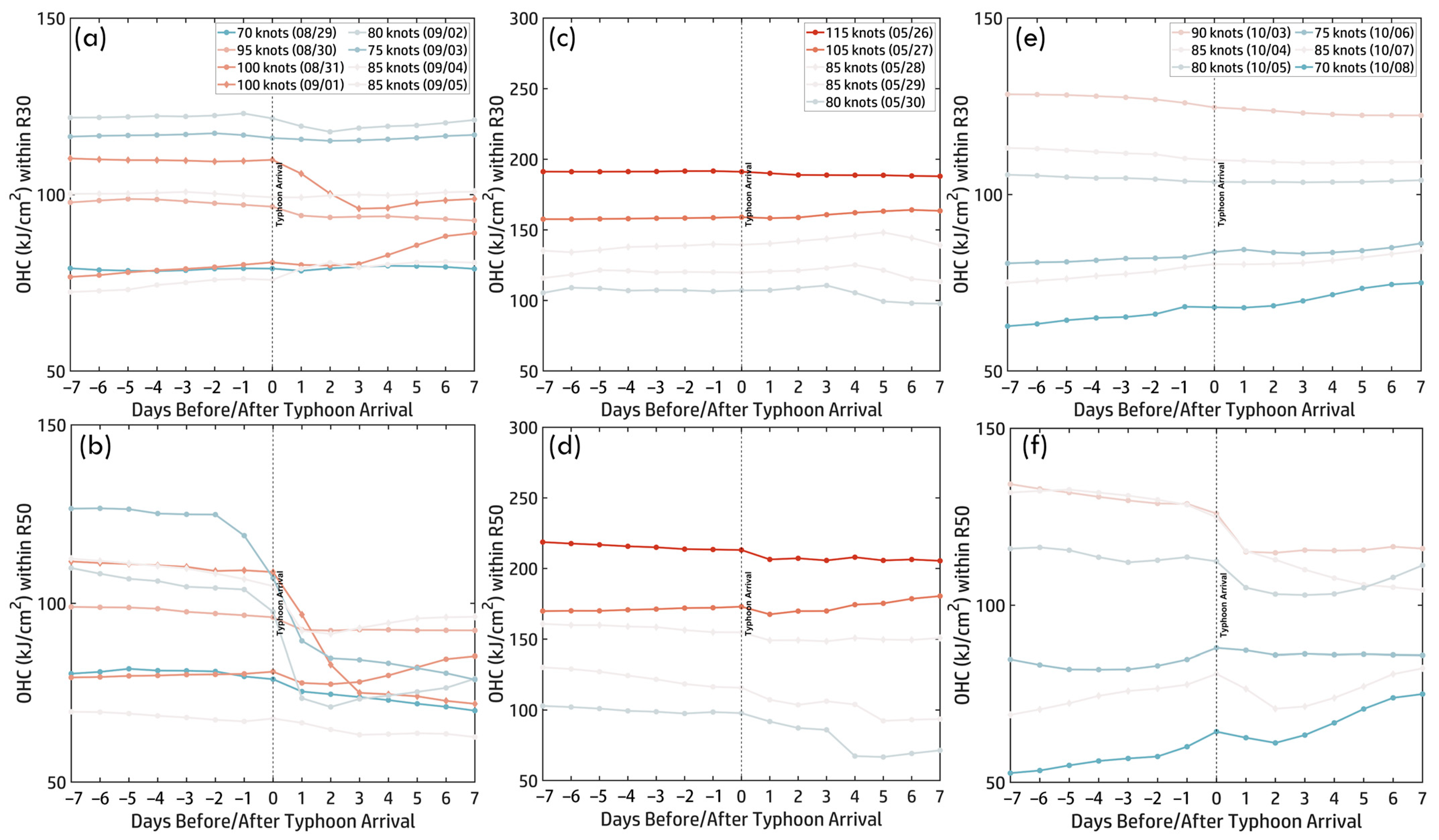
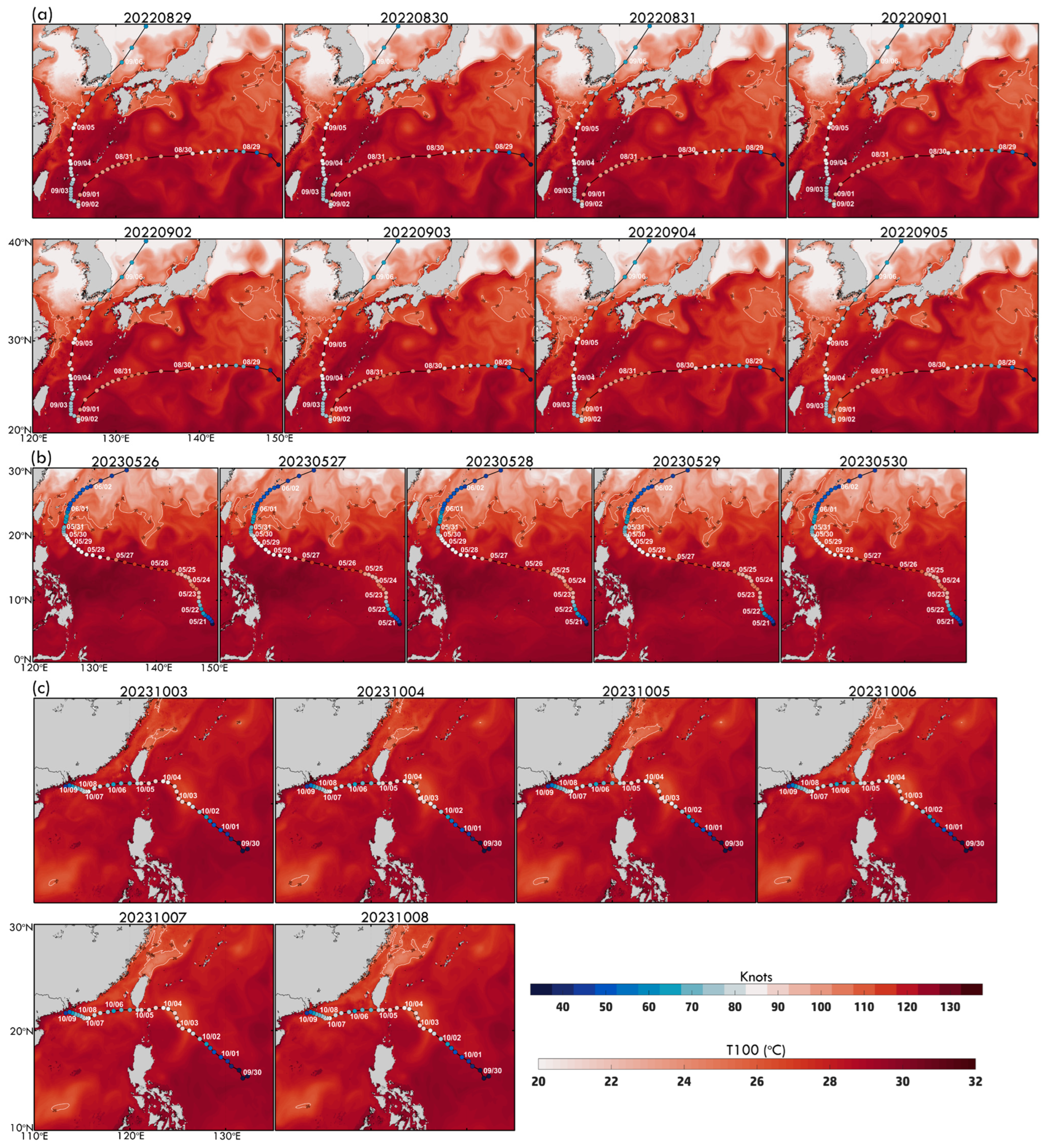
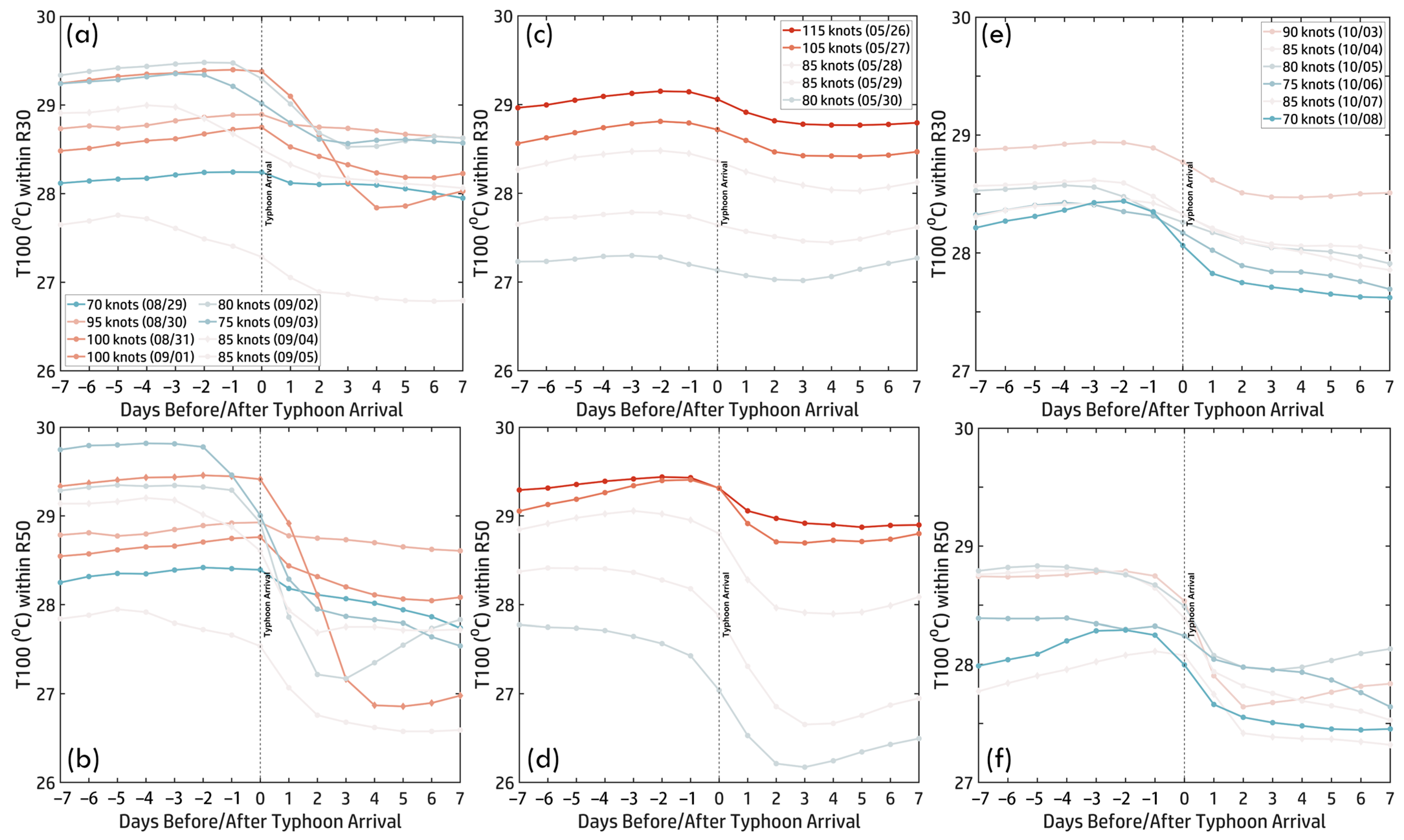
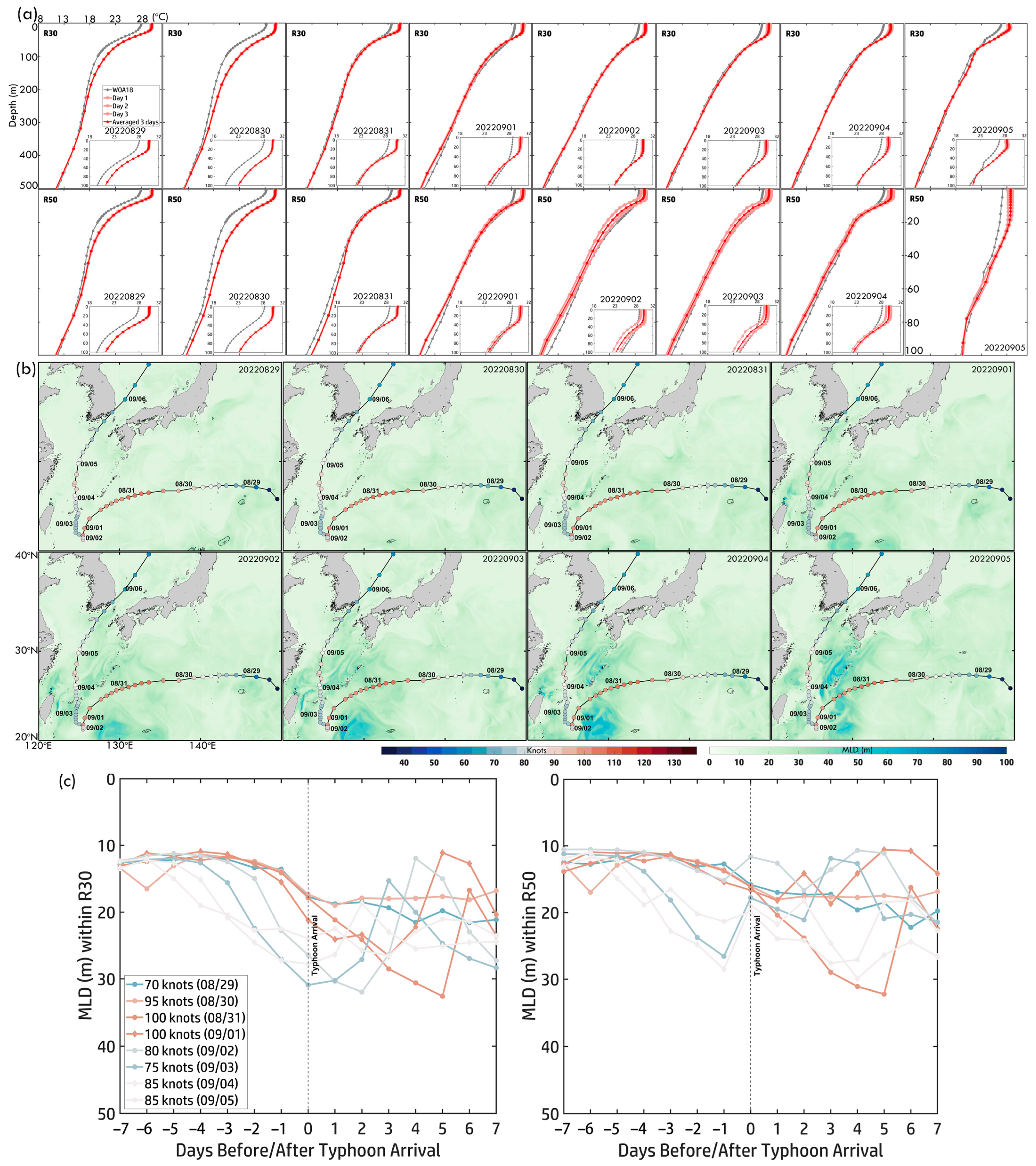
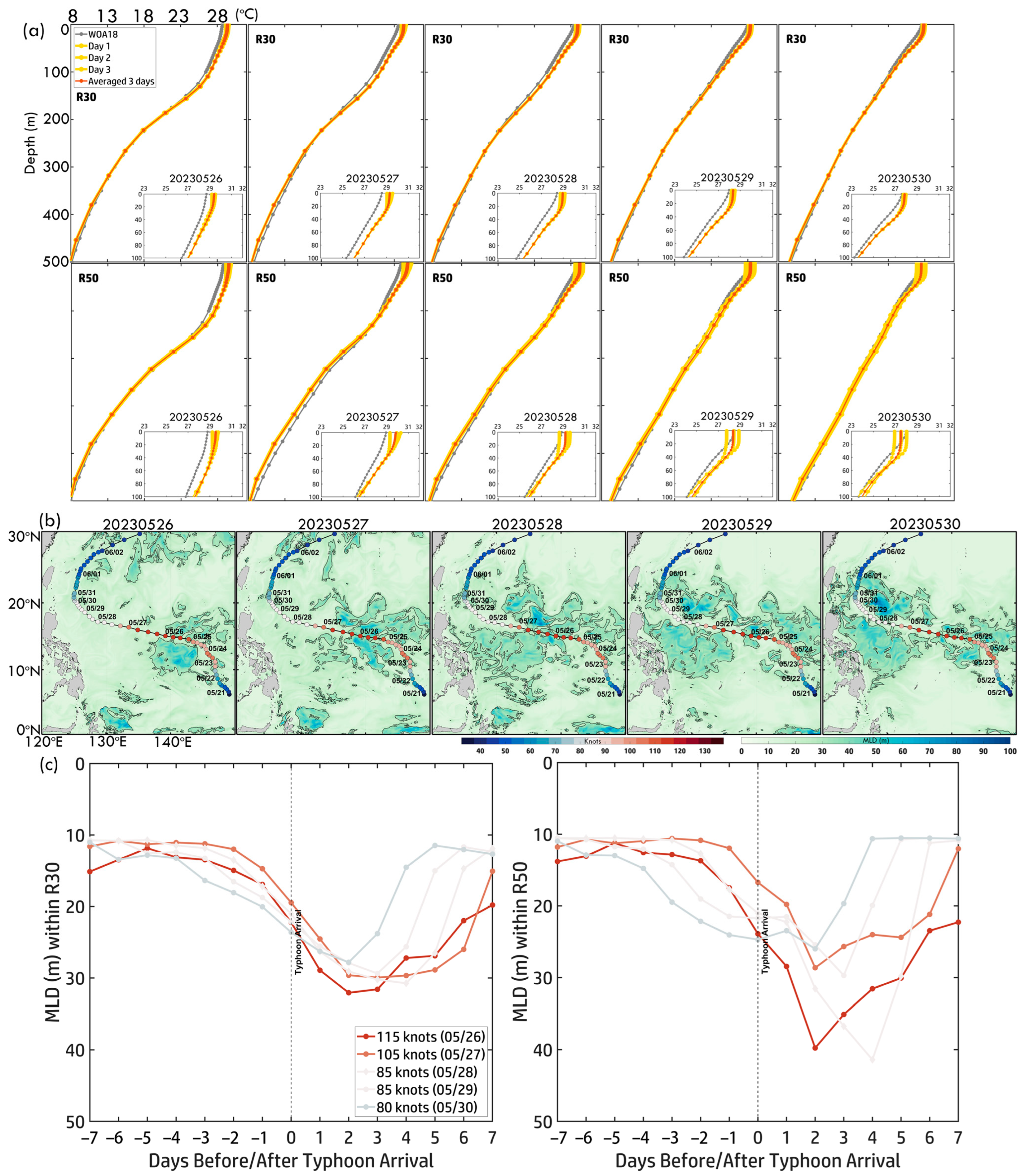
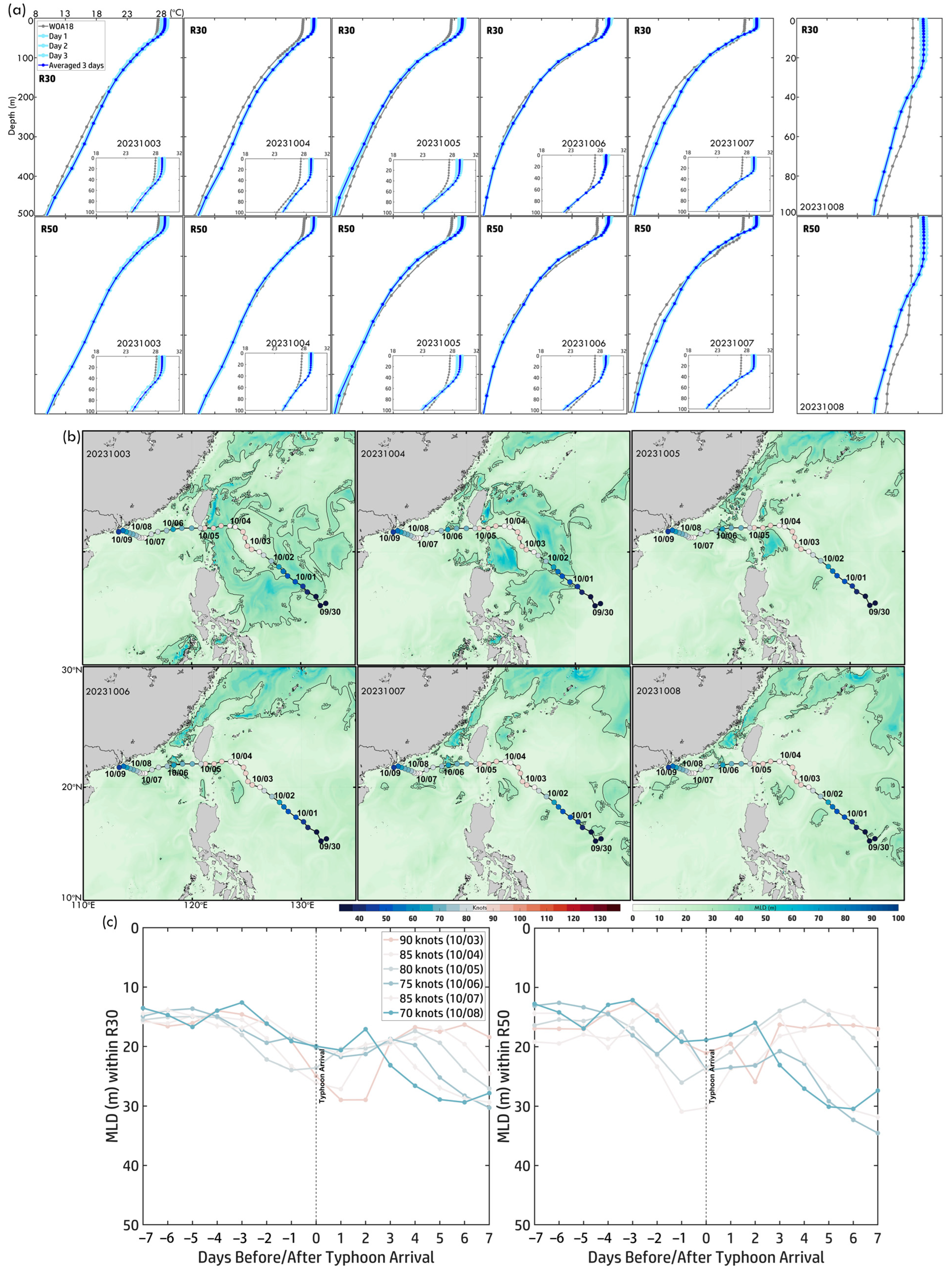
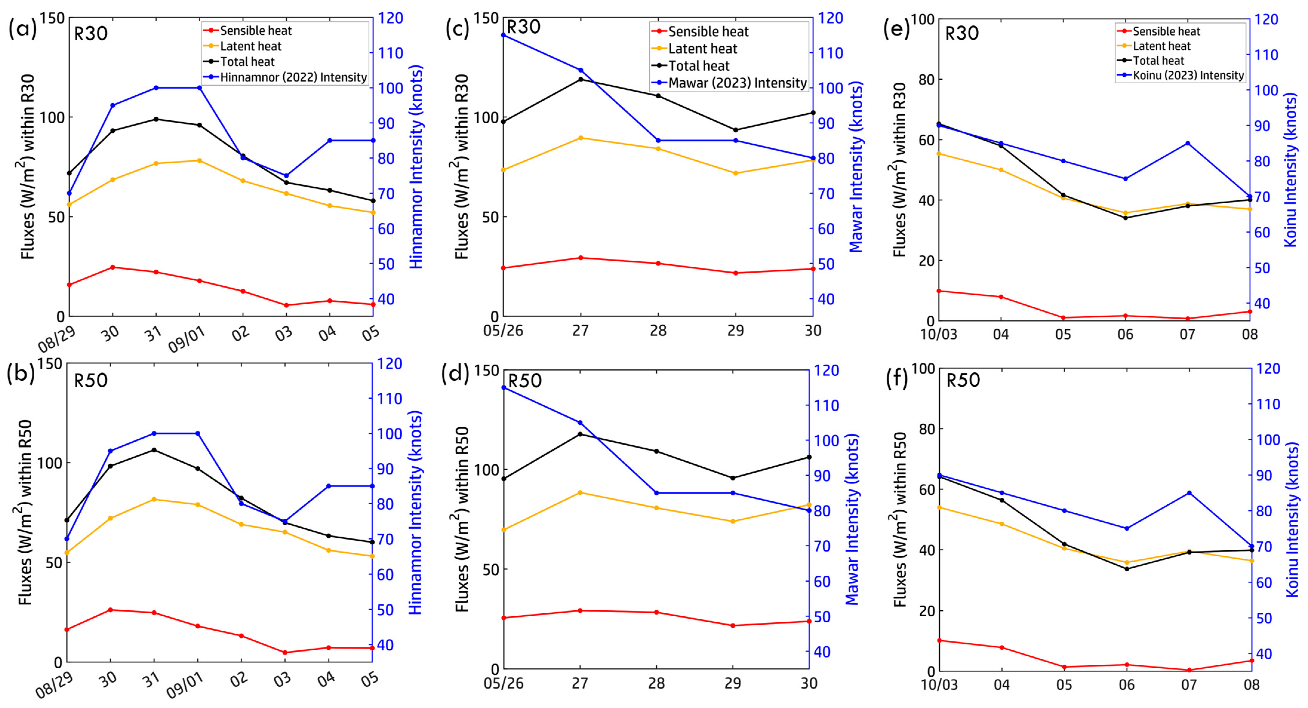
Disclaimer/Publisher’s Note: The statements, opinions and data contained in all publications are solely those of the individual author(s) and contributor(s) and not of MDPI and/or the editor(s). MDPI and/or the editor(s) disclaim responsibility for any injury to people or property resulting from any ideas, methods, instructions or products referred to in the content. |
© 2025 by the authors. Licensee MDPI, Basel, Switzerland. This article is an open access article distributed under the terms and conditions of the Creative Commons Attribution (CC BY) license (https://creativecommons.org/licenses/by/4.0/).