Intelligent Detection of Low–Slow–Small Targets Based on Passive Radar

Abstract

Due to its unique geometric configuration, passive radar offers enhanced surveillance capabilities for low-altitude targets. Traditional passive radar signal processing typically relies on energy accumulation and Constant False Alarm Rate (CFAR) detection. However, insufficient accumulation gain or mismatched statistical models in complex electromagnetic environments can compromise detection performance. To address these challenges, this paper proposes an intelligent target detection method for passive radar. Specifically, a residual network is integrated with a Squeeze-and-Excitation (SE) module, which preserves the powerful feature extraction capabilities of the residual network while improving the model’s ability to adaptively adjust channel weights. This fusion effectively enhances the target detection process. Furthermore, based on the particle swarm algorithm, a gray wolf population search strategy and a multi-target iterative search mechanism are introduced to enable the rapid extraction of time-frequency difference parameters for multiple targets. Both simulation and field experiments demonstrate that the proposed method enables intelligent detection of low–slow–small targets in passive radar, ensuring efficient time-frequency parameter extraction while maintaining a high detection success rate.

1. Introduction

With the rapid advancement of unmanned aerial vehicle (UAV) technology, UAVs have been widely utilized in reconnaissance, surveillance, and aerial photography. However, the increasing frequency of unauthorized UAV flights highlights the urgent need for the development of detection technologies specifically designed for low–slow–small targets. Passive Radar (PR) is a radar system that uses non-cooperative electromagnetic signals for the silent detection of targets in specific areas [1,2]. As a novel radar system, passive radar leverages ambient electromagnetic signals for target detection. Compared to active radar, passive radar offers significant advantages [3,4,5], including strong anti-jamming capabilities, effectiveness against stealth targets, efficient spectrum utilization, and ease of networking and deployment. Given these advantages, passive radar shows significant potential for applications in military reconnaissance, civil aviation, and traffic monitoring [6,7].

As a bistatic radar system, passive radar typically uses two channels for signal reception: the reference channel captures the direct signal from the radiation source, while the surveillance channel receives the target’s reflected echoes [8]. Current target detection methods often enhance SNR through pulse compression or cross-ambiguity accumulation [9], focusing the target’s energy for improved detection. A statistical model is then constructed to generate detection statistics [10,11] based on the principle of ‘energy detection’. The traditional radar target detection process is shown in Figure 1. Traditional detection methods rely on expansion of the available signal dimensions [12]. Examples include one-dimensional CFAR detection for time-domain radar sequences [13] and two-dimensional techniques such as range Doppler moving target detection, 2D CFAR for range azimuth, and space-time (spatial Doppler) processing. However, for the detection of extremely weak target echoes, insufficient accumulation time or complex target echoes causing model mismatches may degrade the detection performance of these methods [14,15]. In addition to the traditional ‘energy accumulation and target detection’ approaches, other techniques also enable effective target detection. In [16], sparse decomposition of direct and echo signals was used, eliminating the need for energy accumulation. In [17], the strengths of RNNs for time-series processing were demonstrated, using LSTM for radar signal prediction and anomaly detection, enabling target detection in cluttered sea environments. Thus, while energy accumulation enhances SNR and aids in target detection, it is not essential for effective detection.

With the improvement of computer performance and the development of neural networks, deep learning has made significant progress in the intelligent information processing of radar data, particularly in addressing classification problems that traditional methods struggle to solve. Target detection is typically framed as a binary hypothesis testing problem [12], where the goal is to determine whether the received signal is a target echo or just noise. Deep learning’s powerful ability to model high-dimensional data enables comprehensive characterization of target echo features, such as RCS fluctuations, target shape, and Doppler frequency. This facilitates the extraction of critical features from target echoes, distinguishing them from background noise and enabling effective detection. The target detection process based on deep learning is shown in Figure 2. Several studies have demonstrated the potential of deep learning in this field. The combination of auto-encoders and convolutional neural networks enables the extraction of deeper feature information [18]. RNNs can capture the correlated features of potential sequences within the time-frequency distribution matrix [19]. By leveraging a dual-channel convolutional neural network to capture multi-dimensional features of targets and clutter in both time and frequency domains, robust target detection can be achieved [20]. In [21], a multi-frame RD spectrum was used, and a sliding window was applied to obtain observation vectors, with detection performed by an MLP detector. By modeling the target echo as a frequency-modulated signal and transforming it into a time-frequency image, GoogLeNet and LetNet can be applied for classification [22]. In [23], a complex-valued UNet network was used to extract features from both the amplitude and phase of the echo to achieve clutter suppression and target detection. In [24], deep neural networks utilized the time-frequency features extracted from the echo cells to achieve detection. Based on the constructed pulse Doppler radar R-D image dataset, a CNN-based detection model was proposed that can accurately detect and locate UAV targets [25]. To address the problem of multi-scale and multi-scene SAR ship detection, a densely connected multi-scale neural network was designed within the Faster R-CNN framework [26]. To address the fact that the features in the range-Doppler map vary over time, 3D-CNN was applied to the 3D representation of time-varying features [27]. In [28], the spectrum of the echo sequence was used as the feature of graph nodes. The adjacency matrix of the graph was computed using the spatiotemporal and power information between the sequences. Classification of the graph nodes was then performed using a graph convolutional network. By using the Visibility Graph (VG) algorithm, the radar echo sequence was modeled as a visibility graph. The graph was then classified using a GCN to achieve detection of weak sea surface targets [29]. In [30], by processing the measured sea clutter data in the time domain, the Laplacian matrix of the graph was constructed, and its maximum eigenvalue was extracted as the detection feature, thereby achieving target detection. It can be observed that deep learning in radar target detection has primarily focused on two-dimensional image processing, where SNR enhancement is achieved through preprocessing techniques such as integral transforms. While these methods improve the target echo SNR before detection, they do not inherently enhance the detector’s capability. Consequently, the detection of low–slow–small targets remains a significant challenge.

The cross-ambiguity function (CAF) [4] is a classical tool for time-delay parameter estimation. However, for accurate estimation of time-frequency differences across various target types, longer detection ranges and faster target velocities expand the search space, significantly increasing the computational load of the CAF. Existing methods of calculating the CAF can be broadly categorized into two types. The first involves exhaustive search. The FFT-based cross-ambiguity function calculation method treats the echo signal and the conjugate of the reference signal, with applied time delay, as a whole and performs FFT processing to traverse the Doppler ambiguity function at specific time delays [31]. The cross-correlation FFT method can obtain the ambiguity function results corresponding to all time delays at the given Doppler frequency [32]. The time-frequency peak search method effectively reduces the search time but still incurs inevitable computational redundancy [33]. Using a multi-population particle swarm optimization algorithm for non-exhaustive search effectively reduces the number of frequency points to search but is prone to falling into local optima [34].

This paper proposes an intelligent detection method for Low, Slow, and Small (LSS) targets. First, deep feature extraction of the radar echo signals is performed using SE-ResNet34 [35]. The channel attention mechanism effectively captures dependencies between the network’s channels, enabling the detection of subtle changes in the radar echoes and accurately determining target presence. The target detection method proposed in this paper leverages the powerful feature extraction capability of deep networks to deeply characterize the background environment and target features, effectively overcoming the issue of statistical model mismatching in traditional digital signal processing. Moreover, this method directly uses the echo signal for network training, without the need for integration or transformation processing. Next, based on the PSO algorithm [34], a gray wolf upper-layer individual guidance and encircling search strategy is introduced, along with a multi-target search mechanism, facilitating the rapid estimation of time-frequency difference parameters for multiple targets. Additionally, the fast time-frequency difference extraction method proposed in this paper further reduces computational redundancy and introduces a multi-target search mechanism, enabling the method to perform multi-target search. Simulation and experimental data demonstrate that the proposed method enables intelligent detection of ‘LLS’ targets and facilitates the rapid extraction of target time-frequency difference parameters.

2. Passive Radar Signal Model

The passive radar system based on DTMB (Digital Terrestrial Multimedia Broadcasting) signals primarily consists of three components: the target, the receiving station, and the transmitting station [8]. The transmitting station is a terrestrial DTMB transmitter with a known position. The receiving station typically uses two channels for signal reception: a reference channel and a surveillance channel. Its structural diagram is shown in Figure 3.

The reference channel is directed toward the transmitting station, primarily receiving the direct path signal as the reference signal ($S_{ref}\left(t\right)$), which can be expressed as

$$S_{ref}\left(t\right)={\alpha }_{0}s\left(t\right)+n_{ref}\left(t\right)$$

(1)

where $s\left(t\right)$ denotes the complex envelope of the DTMB signal, ${\alpha }_0$ denotes the amplitude scaling factor after the DTMB signal propagates through space, and $n_{ref}\left(t\right)$ represents complex Gaussian white noise. The surveillance channel is directed toward the target area, receiving the echo signal ($S_{echo}\left(t\right)$) scattered by the target, which can be expressed as

$$\begin{array}{cc}\hfill S_{echo}\left(t\right)& =S_e\left(t\right)+S_c\left(t\right)+n_{echo}\left(t\right)\hfill \\ \hfill & =\sum _{n=1}^N{\alpha }_{n}s\left(t-{\tau }_n\right)e^{-j2\pi f_{dn}t}+\sum _{m=1}^M{\beta }_{m}s\left(t-{\tau }_m\right)+n_{echo}\left(t\right)\hfill \end{array}$$

(2)

where ${\alpha }_n$ represents the amplitude scaling factor of the DTMB signal after scattering and propagation through space by the n-th target, ${\tau }_n$ denotes the time delay of the echo from the n-th target, $f_{dn}$ represents the Doppler frequency of the n-th target, ${\beta }_m$ represents the complex amplitude of the received clutters, M represents the number of multipath clutters, ${\tau }_m$ represents the time delay of each multipath clutter, N is the number of targets, and $n_{echo}\left(t\right)$ denotes complex Gaussian whiter noise. 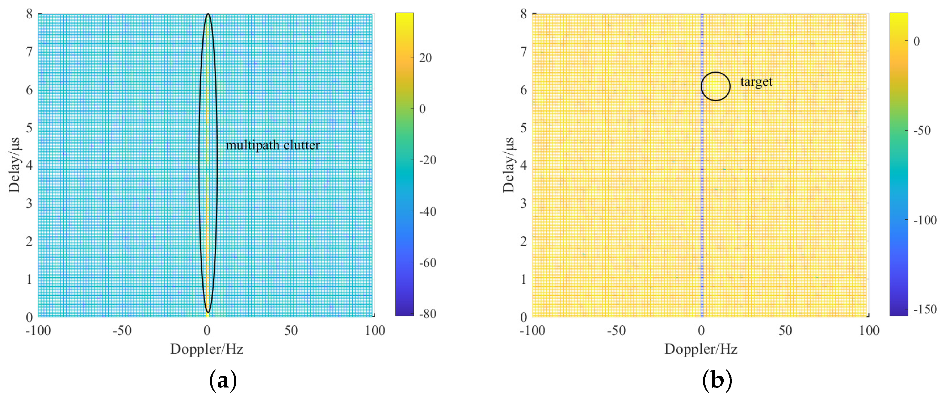By using the ECA clutter suppression algorithm [36], the clutter can be removed, and the echo signal can be expressed as

$${\tilde{S}}_{echo}=S_e\left(t\right)+n_{echo}\left(t\right)=\sum _{n=1}^N{\alpha }_{n}s\left(t-{\tau }_n\right)e^{j2\pi f_{dn}t}+n_{echo}\left(t\right)$$

(3)

As shown in Figure 4, before clutter suppression, the energy of multipath clutter is significantly stronger than that of the target echo, completely masking the target and making detection impossible. However, after applying the ECA algorithm for clutter suppression, the target becomes more prominent.

The cross−ambiguity function is calculated using the received direct path signal and the echo signal and is defined as follows:

$$\chi \left(\tau ,f_d\right)={\int }_0^{T_p}{\tilde{S}}_{echo}\left(t\right)·S_{ref}^{\ast }\left(t-\tau \right)e^{-j2\pi f_{d}t}dt$$

(4)

where $\tau$ denotes the time delay, $f_d$ denotes the Doppler frequency, $T_p$ is the coherent integration time, and $\ast$ represents the complex conjugation operation.

In the ideal case (without noise), it can be observed that the time delay (${\tau }_0$) and Doppler frequency ($f_{d_0}$) of the echo signal relative to the reference signal correspond to the position of the maximum value in the range-Doppler matrix. This indicates that the time delay and Doppler frequency of the target echo can be expressed as follows:

$$\left({\tau }_0,f_{d_0}\right)=\underset{\left(\tau ,f_d\right)}{argmax}\left\{\left|\chi \left(\tau ,f_d\right)\right|\right\}$$

(5)

In modern radar signal processing, radar signals are typically stored in a discrete digital format. The discrete form of Equation (4) is given by

$$\chi \left(l,k\right)=\sum _{n=1}^N{s}_e\left(n\right)·s_r^{*}\left(n-l\right)·exp\left(-j{\displaystyle \frac{2\pi }{N}}kn\right)$$

(6)

where $l=0, 1, \cdots$, L represents the signal time delay unit, $k=-K+1, \cdots , 0, \cdots K-1$, K represents the Doppler frequency unit, and $N=f_s·T_p$ represents the number of sampling points within one coherent integration interval.

3. Intelligent Detection Method for Low–Slow–Small Targets

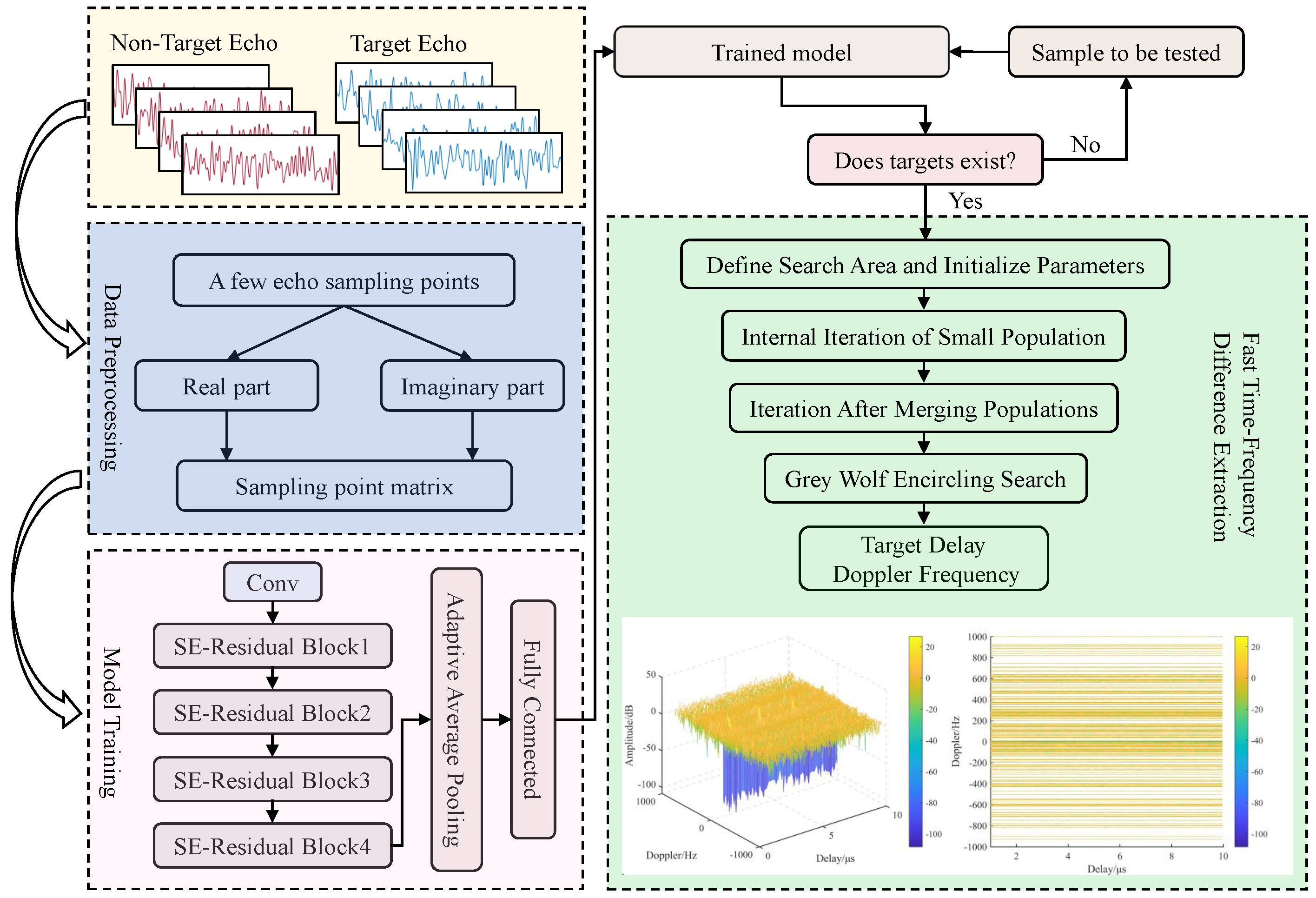
As shown in Figure 5, this paper proposes a deep learning-based method for intelligent detection of low–slow–small targets in passive radar, along with a fast multi−target time−frequency difference extraction method. These two methods are sequential: first, target detection determines if the echo contains a target, providing a basis for parameter extraction; then, the time−delay and Doppler frequency information of the targets are extracted using the multi−target method. The workflow is described as follows:

First, a small number of samples from the received radar echo signal are extracted for the creation of training and testing datasets. Since the radar signal is a complex sequence in practice, its real and imaginary parts are extracted, and the one−dimensional signal is transformed into a two−dimensional form to meet the network input dimension requirements, serving as two input channels for the neural network.

Next, the network is trained using the training set. The SE module’s channel attention mechanism and the residual module’s strong feature extraction capabilities are utilized to perform the ’binary classification’ task for target detection.

Then, the trained network model is used for testing. If a target is detected, the process moves to the fast time−frequency difference extraction step; if no target is detected, a new sample is tested, and the process is repeated.

Finally, the fast extraction of target time-frequency differences is performed. By adding upper-layer individual guidance and an enclosing search strategy, the rapid computation of the ambiguity function is achieved. Additionally, a multi-target search mechanism is incorporated, enabling the proposed algorithm to perform a multi−target search.

3.1. Target Detection Model Based on Channel Attention Mechanism

3.1.1. Squeeze-and-Excitation Blocks

It can be seen from the signal model in Section 2 that when a target is present, the radar echo contains features such as the target’s motion information and RCS scattering variations, which are significantly different from the noise signal alone. In traditional convolutional neural networks, convolutional layers typically process the spatial information of input feature maps independently, while channel information is handled separately within each convolutional channel. Squeeze-and-excitation networks, in contrast, adaptively recalibrate channels, enabling the network to more effectively capture inter-channel dependencies [35].

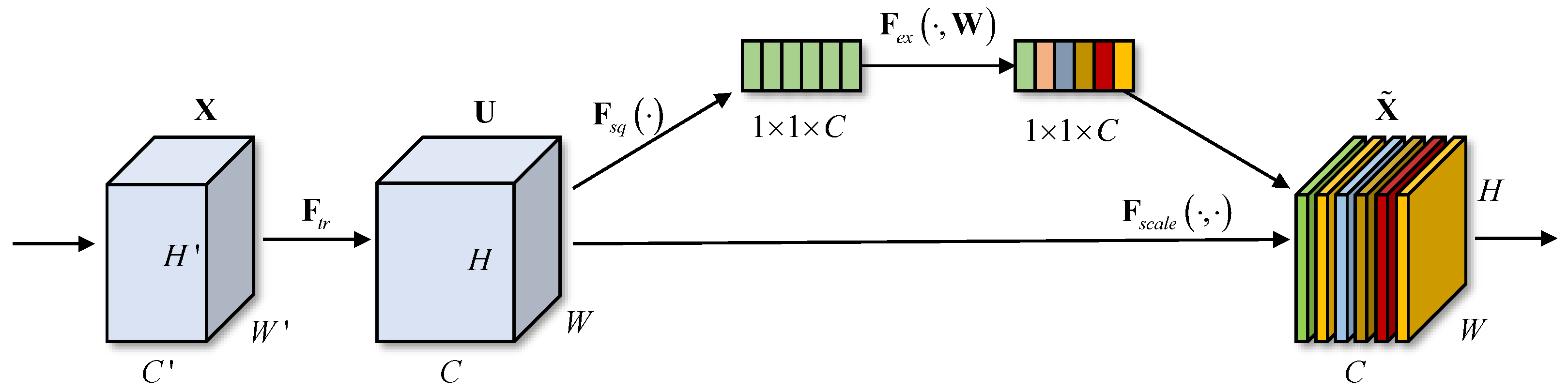
As shown in Figure 6, the key to this network lies in performing the squeeze and excitation operations. First, the network applies global average pooling to the feature map of each channel, and its mathematical formulation is expressed as follows:

$${\mathbf{F}}_{sq}\left({\mathbf{u}}_c\right)={\displaystyle \frac{1}{H\times W}}\sum _{i=1}^H\sum _{j=1}^W{u}_c\left(i,j\right)$$

(7)

This operation ensures that each channel produces a single value, aggregating the global information of each channel and capturing its global feature. Suppose the input feature map is a tensor of size H × W × C, where H and W are the spatial dimensions and C is the number of channels. By performing global average pooling, a vector of size 1 × 1 × C is obtained. In radar echoes, signals that contain targets usually exhibit specific features, such as time delay and Doppler frequency. These features can be represented through the aggregation of global information. This is particularly important for the detection of low, slow, and small targets in radar echoes, as these targets may exhibit weak and localized signal characteristics.

Next, a fully connected layer is employed to learn the weight relationships between channels. The excitation operation is performed on the compressed vector to adaptively adjust and generate the final weight for each channel. The mathematical formulation of this process is expressed as follows:

$$\mathbf{s}={\mathbf{F}}_{ex}\left(\mathbf{z},\mathbf{W}\right)=\sigma \left({\mathbf{W}}_2\delta \left({\mathbf{W}}_1\mathbf{z}\right)\right)$$

(8)

where ${\mathbf{W}}_1$ and ${\mathbf{W}}_2$ are the weight matrices of the fully connected layers, $\sigma$ is the sigmoid activation function, and $\mathbf{z}$ is the output from the squeeze operation. The result, $\mathbf{s}$, is the final adaptive weight vector for each channel. In radar signal processing, certain channels may contain key target features (such as time delay and Doppler frequency), while others may only represent noise. Through training, the SE module can automatically identify and enhance the channels relevant to target detection while suppressing noise or irrelevant channels.

Finally, the feature map of each of channel is multiplied by its corresponding weight, which ‘amplifies’ the important channels and ’suppresses’ the less important ones. Mathematically, this can be expressed as

$${\tilde{\mathbf{x}}}_c={\mathbf{F}}_{scale}\left({\mathbf{u}}_c,s_c\right)=s_c{\mathbf{u}}_c$$

(9)

where ${\mathbf{u}}_c$ is the original feature map for channel c and $s_c$ is the scaling factor for that channel.

In conclusion, the SE module helps the network better focus on key features in small target signals. When Low, slow, and small targets are typically smaller with weaker signals. By enhancing critical channels, the SE module improves the network’s ability to perceive these signals and prevents interference from irrelevant information.

3.1.2. A Brief Introduction to SE-ResNet

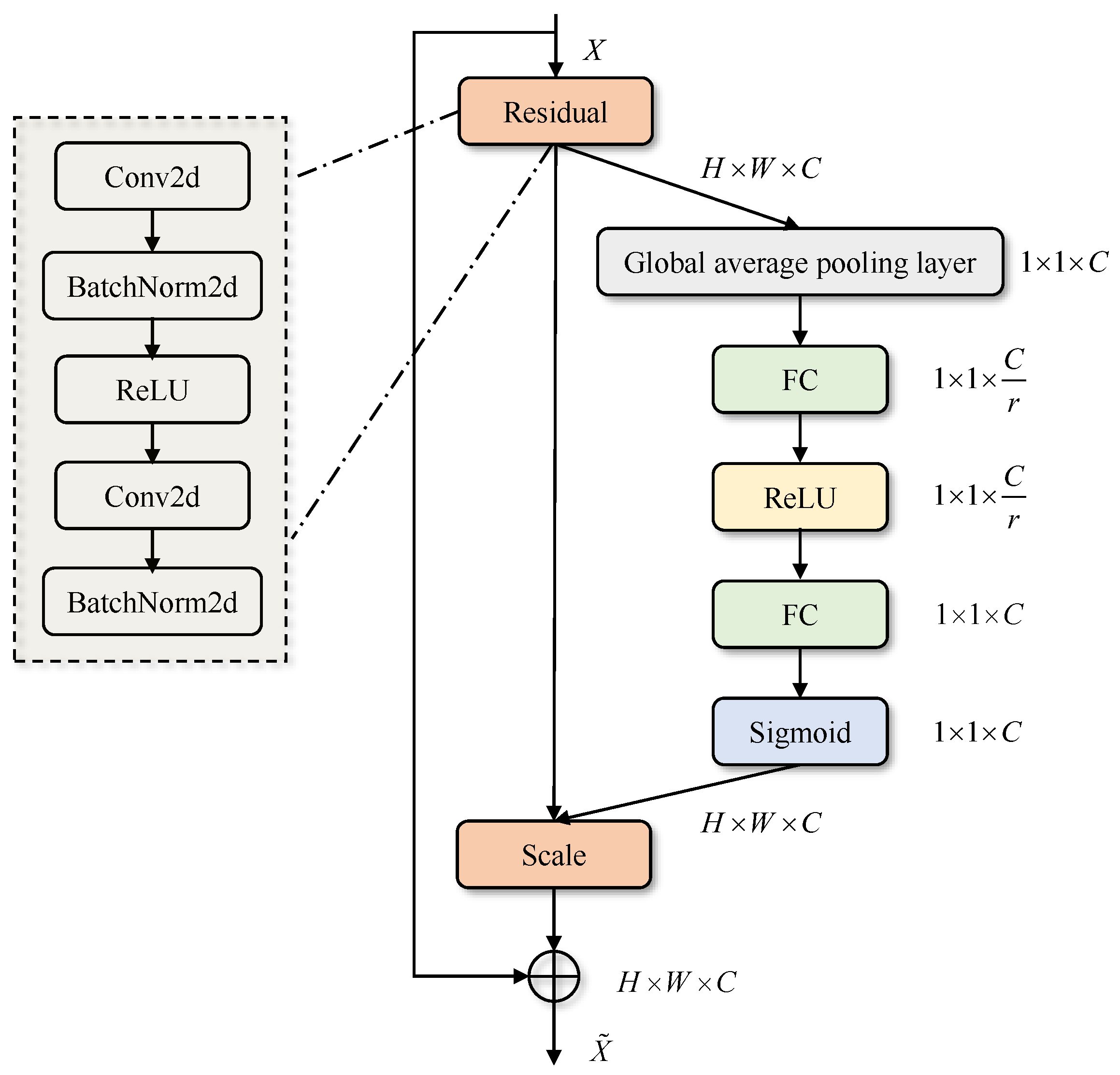
SE-ResNet [35] is a streamlined version of the traditional ResNet [37] that incorporates the squeeze-and-excitation mechanism to enhance channel-wise feature recalibration. The SE-residual block is shown in Figure 7.

The residual module effectively mitigates the vanishing gradient problem that occurs with increasing model depth, ensuring performance improvement as the number of layers increases [37]. In this paper, ResNet34 is combined with a squeeze-and-excitation block.

In various image classification tasks, the combination of the SE block and ResNet has been shown to significantly enhance the performance of the ResNet model. The SE block enables the ResNet model to selectively focus on the most important features, allowing the network to learn more discriminative data representations, thereby improving the model’s prediction accuracy. The specific network structure parameters are presented in

Table 1. SE-ResNet34 parameters.

Layer	Kernel Size	Output Channels	Explanation
Initial Convolution Layer	7 × 7	64	Convolution, BatchNorm, ReLU
Residual Block 1	3 × 3	64	Pooling layer
Residual Block 2	3 × 3	128	Convolution, BatchNorm, ReLU, SE Module
Residual Block 3	3 × 3	256	Convolution, BatchNorm, ReLU, SE Module
Residual Block 4	3 × 3	512	Convolution, BatchNorm, ReLU, SE Module
Global Average Pooling Layer	–	512	Global Average Pooling
Fully Connected Layer	–	2	Output Layer (2 classes for classification)

.

3.1.3. Fast Multi-Target Time-Frequency Difference Extraction Method

This paper presents an efficient method for the rapid extraction of multi-target time-frequency differences in passive radar. By integrating GWO [38] with PSO [34] and incorporating a multi-target iterative search mechanism, the proposed approach enables the accurate and efficient extraction of time delays and Doppler frequency shifts for multiple targets.

If the process of searching for the target’s time-frequency difference is compared to the hunting process of a wolf pack, the position of the prey is analogous to the target’s Doppler frequency, while each individual wolf’s position represents the current Doppler frequency value during the search. The formula for the distance between the target’s Doppler frequency and the current Doppler frequency value during this process is given by (10), and the Doppler frequency update formula is provided in (11).

$$D=\left|C_e\times X_p\left(t_{num}\right)-X_{\omega }\left(t_{num}\right)\right|$$

(10)

$$X_{\omega }\left(t_{num}+1\right)=X_p\left(t_{num}\right)-A_e\times D$$

(11)

where $X_p$ represents the current Doppler frequency value during the search; $t_{num}$ denotes the number of iterations; $X_{\omega }$ indicates the Doppler frequency value after $t_{num}$ iterations; D is the distance between the target’s Doppler frequency and the current doppler frequency; and $A_e$ and $C_e$ are coefficient factors, which are calculated as follows:

$$A_e=2a_1\times r_1-a_1$$

(12)

$$C_e=2\times r_2$$

(13)

where $r_1$ and $r_2$ are random numbers in the range of $\left[0, 1\right]$ and $a_1$ is the convergence factor, which, at iteration $t_{num}$, is defined as follows:

$$a_1=2-t_{num}\times \left(2/T_{num}\right)$$

(14)

where $T_{num}$ is the maximum number of iterations set by the algorithm.

During each iteration, the algorithm updates $\alpha$, $\beta$, and $\delta$ while retaining their position information (current Doppler frequency), ensuring that each iteration is guided by superior individuals. The specific formulas for position updates during this phase are expressed as follows:

$$\left\{\begin{array}{c}{D}_{\alpha }=\left|C_1\times X_{\alpha }\left(t_{num}\right)-X_{\omega }\left(t_{num}\right)\right|\\ D_{\beta }=\left|C_2\times X_{\beta }\left(t_{num}\right)-X_{\omega }\left(t_{num}\right)\right|\\ D_{\delta }=\left|C_3\times X_{\delta }\left(t_{num}\right)-X_{\omega }\left(t_{num}\right)\right|\end{array}\right.$$

(15)

where $D_{\alpha }$, $D_{\beta }$, and $D_{\delta }$ represent the distances between $\alpha$, $\beta$, and $\delta$ and other individuals; $C_1$, $C_2$, and $C_3$ are random vectors; $X_{\alpha }$, $\beta$, and $X_{\delta }$ denote the position of $\alpha$, $\beta$, and $\delta$, respectively; and $X_{\omega }$ represents the position of $\omega$.

Formula (16) defines the step length and direction of $\omega$ moving towards $\alpha$, $\beta$, and $\delta$, while Formula (17) defines the updated position of $\omega$.

$$\left\{\begin{array}{c}{X}_1\left(t_{num}\right)=X_{\alpha }\left(t_{num}\right)-A_1\times D_{\alpha }\\ X_2\left(t_{num}\right)=X_{\beta }\left(t_{num}\right)-A_2\times D_{\beta }\\ X_3\left(t_{num}\right)=X_{\delta }\left(t_{num}\right)-A_3\times D_{\delta }\end{array}\right.$$

(16)

$$X_{\omega }\left(t_{num}+1\right)=\left[X_1\left(t_{num}\right)+X_2\left(t_{num}\right)+X_3\left(t_{num}\right)\right]/3$$

(17)

The particle velocity and position update formulas proposed in [34] are expressed as (18) and (19), respectively:

$$\begin{array}{c}{v}_{ij}\left(t+1\right)=\xi ·\left\{\varpi \times v_{ij}\left(t\right)\right.+c_1{r}_1\left(t\right)\left[p_{ij}\left(t\right)-x_{ij}\left(t\right)\right]\\ +c_2{r}_2\left(t\right)\left[p_{gj}\left(t\right)-x_{ij}\left(t\right)\right]\end{array}$$

(18)

$$x_{ij}\left(t+1\right)=x_{ij}\left(t\right)+v_{ij}\left(t+1\right)$$

(19)

Based on (18), the velocity update formula for the method proposed in this paper is derived as follows:

$$\begin{array}{c}{v}_{ij}\left(t+1\right)=\xi ·\left\{\varpi \times \left[v_{ij}\left(t\right)+X_{\omega ij}\left(t\right)-x_{ij}\left(t\right)\right]\right.+c_1{r}_1\left(t\right)\left[p_{ij}\left(t\right)-x_{ij}\left(t\right)\right]\\ +c_2{r}_2\left(t\right)\left[p_{gj}\left(t\right)-x_{ij}\left(t\right)\right]\end{array}$$

(20)

The velocity update formula exhibits the following characteristics: it retains the contraction factor ($\xi$) to accelerate the algorithm’s convergence speed, preserves the guiding mechanism of individual experience ($p_{ij}\left(t\right)$) and the optimal particle ($p_{gj}\left(t\right)$) from the original algorithm, and incorporates the upper-ranking wolf guidance strategy and encircling search strategy ($X_{\omega ij}\left(t\right)$).

To enhance the multi-target search capability of the algorithm, this paper introduces an iterative peak search mechanism. Specifically, by establishing a historical particle set and an optimal particle set to store searched particles and peaks, the algorithm temporarily excludes previously searched target peaks to avoid interference in subsequent iterations. The specific steps are shown in Algorithm 1.

Algorithm 1 Multi-Fast target time-frequency difference extraction method for passive radar

1: Divide the search area by defining the delay search range as $\left[{\tau }_{min},{\tau }_{max}\right]$ and the Doppler frequency search range as $\left[f_{dmin},f_{dmax}\right]$. Initialize the historical particle set as $particle\_copy=⌀$ and the optimal particle set as $history\_best=⌀$;  2: Initialize the particle population by generating Q particles and dividing them into H equally sized subpopulations ($G_h,h=1,2,\cdots ,H$);  3: Calculate the fitness values of particles that do not intersect with the historical particle set ($particle\_copy$), setting the fitness values of particles that intersect with the optimal particle set ($history\_best$) to zero. Compute the fitness values of the remaining particles based on the historical particle set. Subsequently, update each particle’s individual optimal value ($pbes{t}_q\left(q=1,2,\cdots ,Q\right)$), the global optimal value ($gbes{t}_h\left(h=1,2,\cdots ,H\right)$) for each subpopulation, and the global optimal position ($g_h$) for each subpopulation;  4: Update each particle’s velocity and position according to (18) and (19) while also applying boundary condition handling;  5: Check whether the number of iterations has reached the maximum iteration count ($T_1$) for the subpopulation. If so, proceed to step 6; otherwise, check if the target selection threshold ($\zeta$) has been met. If it has, proceed to step 12; if not, repeat steps 3 to 5;  6: Merge the subpopulations to obtain the global optimal fitness ($gbest$) and the global optimal position (g);  7: Determine whether the target screening threshold ($\zeta$) has been reached. If so, proceed to step 12; otherwise, proceed to step 8;  8: Initialize all particles simultaneously as the initial gray wolf population;  9: Select the three particles with the highest fitness values as the three wolves, $\alpha$, $\beta$, and $\delta$. Then, update the position of particle ($X_q\left(q=1,2,\cdots ,Q\right)$) according to Equations (15)–(17). Subsequently, update the velocity and position of each particle using Equations (20) and (19) while applying boundary condition handing; 10: Calculate the fitness values for particles that do not intersect with the historical particle set ($particle\_copy$), while the remaining particles derive their fitness values directly from the historical particle set. Then, update the global best value ($gbest$) and the global best position (g); 11: Determine whether the maximum number of iterations ($T_{max}$) has been reached. If so, proceed to step 13; otherwise, check if the target selection threshold ($\zeta$) has been met. If it has, proceed to step 12; if not, repeat steps 8 to 11; 12: Save all currently discovered particles to the $particle\_copy$ and store the global best particle in the optimal particle set ($history\_best$). Then, repeat steps 2 to 12; 13: Determine whether the target selection threshold ($\zeta$) has been met. If so, proceed step 12; otherwise, output the $particle\_copy$ as the result of the cross-ambiguity function calculation.

3.1.4. Computational Complexity Analysis

As shown in

Table 2. Comparison of the number of complex multiplications.

Method	Complex Multiplication Computation
Cross-corelation FFT method	$2K\times \left[N+{\displaystyle \frac{3N}{2}}{log}_2\left(N\right)\right]$
Method proposed in [34]	$Gen\times Q\times \gamma \times \left[N+{\displaystyle \frac{3N}{2}}{log}_2\left(N\right)\right]$
The proposed method	$M\times \left(Ge{n}_{pro1}\times Q_{pro1}+Ge{n}_{pro2}\times Q_{pro2}\right)\times \left[N+{\displaystyle \frac{3N}{2}}{log}_2\left(N\right)\right]$

, $2K$ is the number of Doppler frequency bins in the RD spectrum obtained by the cross-correlation FFT method. $Gen$ represents the number of algorithm iterations, N is the signal length, Q is the population size, and $\gamma$ is the repetition factor for multiple particles updating to the same Doppler frequency. M is the number of targets, $Ge{n}_{pro1}$ is the number of iterations for the small population, $Q_{pro1}$ is the size of the small population, $Ge{n}_{pro2}$ is the number of iterations for the gray wolf population, and $Q_{pro2}$ is the size of the gray wolf population.

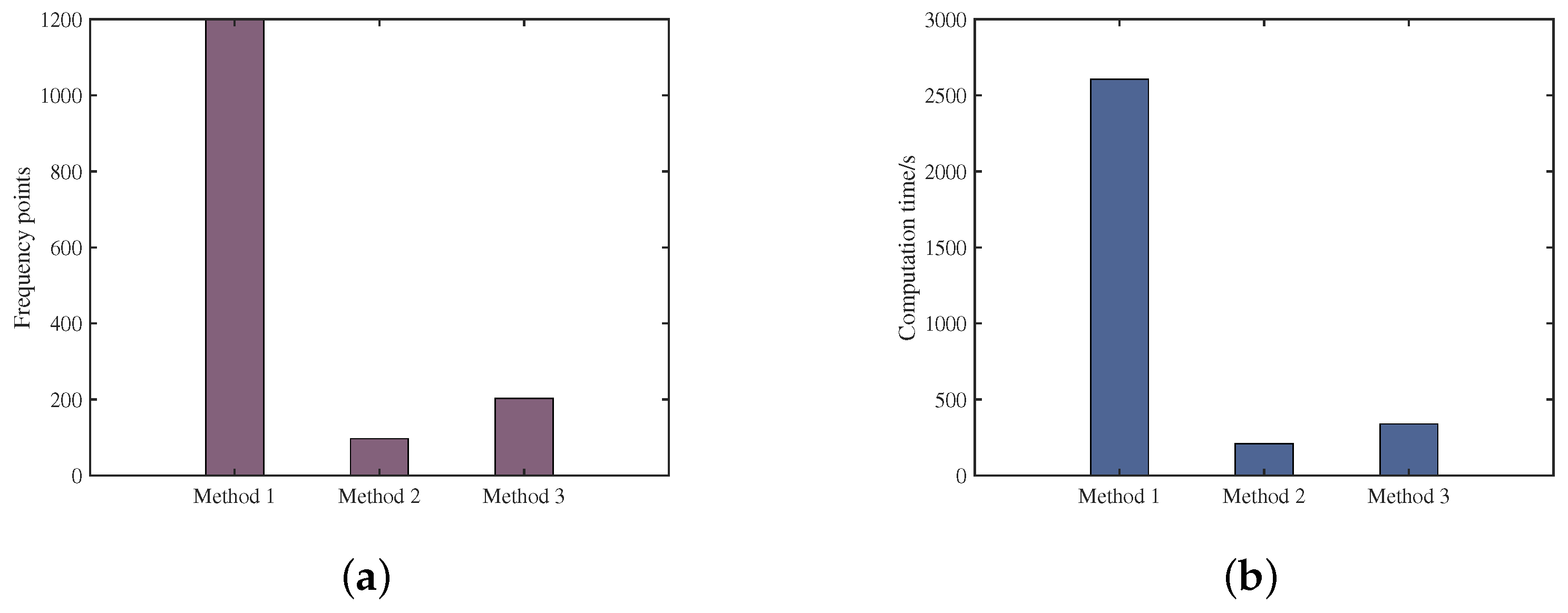
Since, in practical situations, the Doppler frequency range of the targets is unknown, the value of K is set as large as possible to ensure that all targets can be searched. Therefore, based on the algorithm’s principles, we have $M\times \left(Ge{n}_{pro1}\times Q_{pro1}+Ge{n}_{pro2}\times Q_{pro2}\right)$ < $2K$ and $M\times \left(Ge{n}_{pro1}\times Q_{pro1}+Ge{n}_{pro2}\times Q_{pro2}\right)$ > $Gen\times Q\times \gamma$. As a result, the method proposed in this paper reduces the computational complexity compared to the cross-correlation FFT method. However, it increases computational complexity compared to the method proposed in reference [34] due to the added iterative search mechanism, which ensures the multi-target search capability of the proposed method.

4. Experimental Results

4.1. Performance of SE-ResNet34 in Passive Radar Target Detection

4.1.1. Dataset Construction

The original data used in this experiment is obtained from field tests. A low, slow, and small target detection scenario based on passive radar is constructed, utilizing the Beigaofeng TV tower in Hangzhou as the signal source. The signal type is DTMB, with a bandwidth of 7.56 MHz and a carrier frequency of 530 MHz. The receiving station is situated in farmland in Jiaxing, where a large antenna array is employed to capture both the reference signal and the target echoes. The receiver’s sampling rate is 25 MHz. To control the SNR of the target echo, based on the passive radar echo signal model, time delay and Doppler frequency shifts are applied to the direct signal to simulate the target echoes.

Based on the constructed passive radar signal model, 60,000 training samples are generated. The signal length is set to $N=1444$, with half of the samples labeled as $H_0$ (containing only noise) and the other half as $H_1$ (containing both target and noise). The expected outputs are 0 for $H_0$ samples and 1 for $H_1$ samples. In constructing the training set for $H_1$ samples, the following assumptions are made: The number of targets is randomly generated within the range of $\left[1,5\right]$. Each target’s initial time delay is randomly generated within the range of $\left[1,40\right]$ μs, and each target’s Doppler frequency is randomly generated within the range of $\left[-350,350\right]\mathrm{Hz}$. The SNR is set to one of the following values: $\left[-7,-9,-11,-13,-15,-17\right]\mathrm{dB}$. For each SNR value, 5000 data samples are generated, resulting in a total of 30,000 $H_1$ samples. Next, Test Set 1 is created with 18,000 samples, ensuring that the class distribution in this test set is consistent with that of the training set.

To evaluate the generalization ability of the model, Test Set 2 is constructed. The number of targets is randomly generated within the range of $\left[1,5\right]$. Each target’s initial time delay and Doppler frequency are generated in the same manner as described earlier. The echo SNR values are set to range from 0 dB to 20 dB, with each SNR value generating 1500 $H_1$ samples and 1500 $H_0$ samples. Therefore, for each SNR value, a total of 3000 samples are generated.

4.1.2. Evaluation Metrics

In handing binary classification problems, the test data are divided into two categories: positive and negative samples. As shown in Figure 8, TP (True Positive) refers to correctly classified positive samples, while FP (False Positive) refers to negative samples incorrectly classified as positive. TN (True Negative) represents correctly classified negative samples, and FN (False Negative) refers to positive samples incorrectly classified as negative.

The formula for accuracy is defined as follows:

$$\mathrm{Accuracy}={\displaystyle \frac{TP+TN}{TP+TN+FP+FN}}$$

(21)

The formula for the detection rate (also called recall) is defined as follows:

$$\mathrm{Detection}\mathrm{Rate}\left(\mathrm{Recall}\right)={\displaystyle \frac{TP}{TP+FN}}$$

(22)

The formula for the false alarm rate is defined as follows:

$$\mathrm{False}\mathrm{Alarm}\mathrm{Rate}={\displaystyle \frac{FP}{FP+TN}}$$

(23)

4.1.3. Network Effectiveness Analysis

During the training process, the backpropagation algorithm is employed to minimize the cross-entropy loss function. The hyperparameters are set as follows: the batch size is 64, the model is trained for 500 epochs, the learning rate is initialized at 0.001, and the Adam optimizer is utilized for optimization.

As shown in Figure 9, the network’s loss curve decreases rapidly during the first ten epochs. As the number of iterations increases, the loss gradually approaches zero and stabilizes. Concurrently, the model’s accuracy rises sharply, reaching approximately 99.5% within the first ten epochs. After 50 epochs of training, the accuracy on the training set approaches 100%, and it remains stable at this level throughout the remaining training process.

The performance of the network on Test Set 1 is shown in Figure 10. As illustrated, in the binary classification task discussed in this paper, when the target is absent, the probability of the network correctly predicting the result is 98.2%, while the probability of incorrect prediction is 1.8%; when the target is present, the probability of the network correctly predicting the result is 95.51%, while the probability of incorrect prediction is 4.49%. These results indicate that SE−ResNet34 demonstrates significant effectiveness and feasibility in passive radar target detection.

4.1.4. Experiment on the Relationship Between Accuracy and SNR

To further evaluate the feasibility and generalization ability of the network in the target detection task, Test Set 2 was used to assess how the accuracy of the network model varies under different SNR conditions. The experimental results are shown in Figure 11.

As shown in Figure 12, when the SNR is relatively high, such as at $-5\mathrm{dB}$ and $-10\mathrm{dB}$, when the target is present, the probability of the network correctly predicting the result is 100%; when the target is absent, only a small number of samples is misclassified, with a probability of approximately 1% to 2%. The overall accuracy is approximately 99%.

However, as the echo SNR decreases, the network’s probability of detecting positive samples also decreases. This trend is particularly noticeable when the SNR is very low, as the echo signal becomes increasingly dominated by noise. For example, when the SNR is −20 dB and the target is present, the probability of the network making a correct prediction is only 23.6%. Under these conditions, it becomes challenging for the network to effectively distinguish between the actual target features and the noise. As a result, detection accuracy significantly drops when the echo SNR is low.

4.1.5. Comparison with Other Deep Learning Networks

To demonstrate the superiority of the SE-ResNet34 model, this paper uses SE-ResNet18, ResNet34, ResNet18, VGG-16 [39], and SENet as benchmark models for comparison. All models are trained using the same set of parameters, including learning rate, optimizer, and others. The test sets used for the comparison experiments are Test Set 1 and Test Set 2.

Table 3. Computational costs of different methods.

Model	Total Params	Estimated Total Size	Average Training Time
SENet (7 blocks)	1,810,434	85.67 MB	49.8 s/epoch
ResNet18	11,169,282	44.81 MB	26.5 s/epoch
ResNet34	21,277,442	81.17 MB	41.3 s/epoch
SE-ResNet18	11,261,442	48.03 MB	29.8 s/epoch
SE-ResNet34	21,434,626	90.49 MB	50.1 s/epoch
VGG−16	29,839,618	113.42 MB	71.8 s/epoch

presents the computational costs of different deep learning networks. It can be observed that after adding the SE module, the increase in both the parameter count and computational cost of the residual networks is minimal. Adding the SE module improves the model’s feature representation ability while keeping the parameter count under control. By comparing SE−ResNet18 with SE−ResNet34, it can be observed that as the network depth increases, the number of parameters grows significantly. VGG−16 has more total parameters compared to SE−ResNet, but its accuracy is lower than that of the latter. When computational resources permit, it is acceptable to trade computational resources for improved detection accuracy.

From the comparison results in

Table 4. Performance comparison of different models.

Model	Accuracy	Detection Accuracy	False Alarm Rate
SENet (7 blocks)	86.27%	81.54%	9%
ResNet18	90.69%	87.92%	6.54%
ResNet34	90.46%	86.78%	5.86%
SE-ResNet18	94.34%	93.29%	4.61%
SE-ResNet34	96.86%	95.51%	1.8%
VGG−16	91.29%	88.46%	5.88%

, it can be observed that SE-ResNet34 achieves the best performance in terms of accuracy, detection accuracy, and false alarm rate. However, due to its larger number of parameters, the average training time is longer, although still within an acceptable range. Overall, SE−ResNet34 shows outstanding performance in passive radar target detection.

As shown in Figure 13, as the SNR decreases, the accuracy of all networks declines. Among them, SE−ResNet34 maintains the highest accuracy across a broad range of SNR values. SE−ResNet18 exhibits sightly lower accuracy due to its shallower architecture compared to SE−ResNet34. However, the increase in the number of parameters in SE−ResNet34, resulting from its deeper structure, does not significantly affect its performance. In contrast, ResNet18, ResNet34, and SENet lack a channel attention mechanism and residual structure, which limits their ability to effectively extract deep features.

4.2. Experimental Study on the Rapid Extraction of Time-Frequency Differences

After performing target detection on the test signal using the SE−ResNet34 network model, rapid time−frequency difference estimation is applied to signals identified as containing a target. A series of experiments are conducted to validate the effectiveness and efficiency of the proposed method.

Assuming the echo contains two targets with SNRs of −15 dB and −14 dB, respectively, the time delay of target 1 is 18 μs, and its Doppler frequency is 145 Hz, while the time delay of target 2 is 36 μs, and its Doppler frequency is −305 Hz. The accumulation time is 0.5 s. Given the absence of prior information about the targets, a wide-range search for time delay and Doppler frequency is necessary when using the cross-ambiguity function for time-frequency difference estimation. The time-delay search range is set to [0, 100] μs, and the Doppler frequency search range is set to [−1000, 1000] Hz, with a total of 1000 frequency points.

Figure 14b,d,f display the corresponding time-delay Doppler-plane accumulation results, where each line represents the total ambiguity function results within the time-delay search range at a specific frequency point and the unit of the color bar is dB. The number of computation frequency points in these case are 1000, 59, and 92, respectively. When two targets are present, both the cross-correlation FFT method and the proposed method are able to detect all targets, with the computational complexity of the proposed method being approximately 1/10 that of the cross-correlation FFT method. The method proposed in [34] has the lowest computation complexity but lacks the ability to detect multiple targets, resulting in target misdetection. The proposed method provides the best detection performance while maintaining an acceptable computational load.

A Monte Carlo experiment was conducted on the ambiguity function calculation process, with each experiment repeated 100 times. Statistics were performed on the average number of frequency points, average computation time, and multi-target search success rate to provide a comprehensive measure of the proposed algorithm’s performance. The experimental results are shown in

Table 5. Comparison of different methods for two targets.

Method	Average Frequency Point	Average Computation Time	Multi-Target Search Success Rate
Cross-corelation FFT method	1000	2128.12 s	100%
Method proposed in [34]	54	112.25 s	19%
The proposed method	141	248.67 s	100%

. The definition of the multi-target search success rate is expressed as follows:

$$P_d={\displaystyle \frac{\mathrm{Times}\mathrm{all}\mathrm{target}\mathrm{peaks}\mathrm{are}\mathrm{detected}}{\mathrm{Number}\mathrm{of}\mathrm{Monte}\mathrm{Carlo}\mathrm{simulations}}}\times 100\%$$

(24)

As shown in Table 5, although the method proposed in [34] has the lowest computation time, it is unable to perform multi-target searches and fails to detect all targets. In contrast, the method proposed in this paper accurately detects all targets, with a computational cost approximately 1/8 of that of the cross-correlation FFT method. The proposed method significantly reduces the number of frequency search points while maintaining detection accuracy.

Next, the number of targets is varied, with the parameters for each target specified in

Table 6. Target parameter settings.

Parameter	Target 1	Target 2	Target 3	Target 4	Target 5
Delay/μs	2	12	31	18	26
Doppler/Hz	50	−80	154	−206	100
SNR/dB	−10	−15.5	−15	−14	−13

. Monte Carlo experiments are performed for each target using the previously described search process, generating the search results for different methods with varying target quantities.

As shown in

Table 7. Impact of the number of targets on algorithm performance.

Number of Targets	Method	Average Frequency Point	Average Computation Time	Multi-Target Search Success Rate
1	Cross-correlation FFT	1000	2130.95 s	100%
	Method proposed in [34]	49	107.43 s	100%
	The proposed method	53	115.79 s	100%
2	Cross-correlation FFT	1000	2128.12 s	100%
	Method proposed in [34]	54	112.25 s	19%
	The proposed method	141	248.67 s	100%
3	Cross-correlation FFT	1000	2120.19 s	100%
	Method proposed in [34]	51	110.16 s	6%
	The proposed method	165	273.61 s	98%
4	Cross-correlation FFT	1000	2127.94 s	100%
	Method proposed in [34]	55	112.89 s	0%
	The proposed method	218	359.19 s	95%
5	Cross-correlation FFT	1000	2128.21 s	100%
	Method proposed in [34]	52	111.84 s	0%
	The proposed method	238	380.67 s	97%

, after varying the number of targets, the method proposed in [34] has the fewest frequency points and the shortest computation time but lacks multi-target detection capability, making it unsuitable for practical use. The proposed method achieves nearly 100% multi-target search success and significantly reduces the number of frequency points compared to the traditional method, and the increased computation time is acceptable.

As shown in Figure 15, as the number of targets increases, the proposed method’s frequency-point count rises but remains lower than that of the cross-correlation FFT method. The method proposed in [34] rapidly loses multi-target search success as the number of targets increases, failing to detect all targets. In conclusion, the proposed method maintains strong multi-target detection capability while significantly reducing computation.

4.3. Experiment with Measured Data

The field test scenario follows the description in Section 4.1, where DJI drones are flown at low altitude to serve as the targets for detection. First, the received echoes are processed using DBF at the receiver to enhance the target echo energy. Then, clutter suppression is applied to minimize the impact of environmental clutter. Finally, the processed echoes are used to construct the measured dataset. The training set consists of 3000 samples with targets and 3000 samples without targets. The test set includes 1000 samples with targets and 1000 samples without targets. Each sample consists of 1444 sampling points.

The data are preprocessed and fed into the network model for target detection. The resulting confusion matrix for the test results is shown in Figure 16. As shown in Figure 16, the confusion matrix validates the effectiveness of the network model. When the target is absent, the probability of the network correctly predicting the result is 99.1%, while the probability of incorrect prediction is 0.9%; when the target is present, the probability of the network correctly predicting the result is 96.8%, while the probability of incorrect prediction is 3.2%.

Now, the drones perform predefined maneuvers to evaluate the model’s effectiveness. The total data collection time is set to 40 s, with the drones ascending vertically from 0 to 18 s, followed by radial motion toward the receiver array from 18 to 40 s. The theoretical target status and detection results are shown in Figure 17, assuming the drones are in the ‘target present’ state during radial motion.

As shown in Figure 17, the detection results of the deep learning-based target detection network are close to the theoretical scenario. The fluctuation around 18 s occurs due to the transition of the drones from vertical ascent to radial motion. The target detection method based on traditional coherent accumulation followed by CFAR detection in passive radar also successfully detects the target. However, the overall computational time is too high and does not meet real-time requirements.

The time required by the proposed method includes the duration for testing with the trained model (T1) and the time for performing time-frequency difference extraction (T2). Since T1 is negligible compared to T2, only T2 is considered here. The time required by the traditional passive radar target detection method is mainly concentrated in the coherent accumulation step, i.e., the cross-correlation FFT algorithm described in this paper. A comparison of the time taken using the measured data is shown in Figure 18.

The cross-correlation accumulation time is 0.6 s, with a delay search range of $\left[1,10\right]$ μs and a Doppler search range of $\left[-1000,1000\right]\mathrm{Hz}$. The environment includes three drones as the detection targets. As shown in Figure 18, Method 1 is the cross-correlation FFT algorithm, Method 2 is the method proposed in [34], and Method is the time-frequency difference extraction algorithm proposed in this paper. The frequency points for the three methods are 1200, 97, and 203, and the computation times for three methods are 2605.76 s, 210.61 s, and 338.98 s, respectively. As shown in Figure 19, the cross-correlation FFT method detects all three targets but with significant computational redundancy, while the method proposed in [34] detects only two targets. The proposed method detects all three targets while significantly reducing computation, making it suitable for practical applications.

5. Discussion

In real-world applications, the proposed system may encounter several limitations that could impact its performance. Some of the most common factors include the following:

First, adverse weather conditions such as heavy rain, snow, or fog can significantly degrade the performance of radar and other sensing systems. Radar signals may be heavily attenuated by precipitation, resulting in reduced detection capabilities.

Next, due to its bistatic configuration, the passive radar system imposes strict terrain requirements. Obstructions such as mountains and tall buildings can block both the echo signal and even the direct signal reception. Additionally, during long-range detection, the Earth’s curvature may hinder the reception of reference signals.

Finally, in practical applications, environmental parameters evolve over time. As a result, the features extracted by the network may no longer be applicable to the current conditions. Therefore, periodic data collection and network retraining are necessary to maintain optimal performance.

6. Conclusions

This paper proposes an intelligent target detection method based on passive radar. By incorporating a residual network architecture with a channel attention mechanism to construct SE-ResNet34, the proposed method effectively determines the presence or absence of targets in echo signals. The time-frequency differences of the targets are then efficiently extracted, enabling the successful completion of the passive radar target detection task. Simulation experiments demonstrate that the SE-ResNet34 model achieves a high target detection rate in the binary classification task. Furthermore, under low-SNR conditions, the accuracy of the proposed model surpasses that of the compared models. The simulation experiments also indicate that the proposed time-frequency difference extraction method is capable of multi-target time-frequency difference search, achieving a success rate above 95%, while significantly reducing the number of search frequency points. Field tests confirm that the proposed method performs robustly in real-world environments, highlighting its significant potential for engineering applications.

Although SE-ResNet34 maintains high accuracy, it also requires considerable computational resources. Developing a lightweight target detection network will be a key focus of future research. Moreover, a deeper analysis of the model’s generalization to larger datasets from real-world field experiments will be an important direction for further investigation. The proposed rapid time-frequency difference extraction method still exhibits computational redundancy compared to the methods compared in this paper. Further reducing the number of search frequency points and improving search efficiency will be important areas for future work. Moreover, the practical performance of this method needs to be further explored as the number of targets increases.