Multi-Temporal and Multi-Resolution RGB UAV Surveys for Cost-Efficient Tree Species Mapping in an Afforestation Project

Abstract

Accurate, cost-efficient vegetation mapping is critical for managing afforestation projects, particularly in resource-limited areas. This study used a consumer-grade RGB unmanned aerial vehicle (UAV) to evaluate the optimal spatial and temporal resolutions (leaf-off and leaf-on) for precise, economically viable tree species mapping. This study conducted in 2024 in Kasho, Bannu district, Pakistan, using UAV missions at multiple altitudes captured high-resolution RGB imagery (2, 4, and 6 cm) across three sampling plots. A Support Vector Machine (SVM) classifier with 5-fold cross-validation was assessed using accuracy, Shannon entropy, and cost–benefit analyses. The results showed that the 6 cm resolution achieved a reliable accuracy (R² = 0.92–0.98) with broader coverage (12.3–22.2 hectares), while the 2 cm and 4 cm resolutions offered higher accuracy (R² = 0.96–0.99) but limited coverage (4.8–14.2 hectares). The 6 cm resolution also yielded the highest benefit–cost ratio (BCR: 0.011–0.015), balancing cost-efficiency and accuracy. This study demonstrates the potential of consumer-grade UAVs for affordable, high-precision tree species mapping, while also accounting for other land cover types such as bare earth and water, supporting budget-constrained afforestation efforts.

1. Introduction

Accurate vegetation mapping is vital for forest management, biodiversity conservation, and ecosystem restoration [1]. Since it furnishes fundamental data essential for estimating carbon sequestration—encompassing various vegetation types, canopy height, structure, etc.—it concurrently acts as a significant tool for assessing carbon sequestration potential [2], which is essential for climate change mitigation and achieving the Sustainable Development Goals (SDGs). Desertification threatens arid, semi-arid, and dry sub-humid regions, causing significant losses of water, vegetation, and wildlife [3,4]. From 1961 to 2013, drought-affected drylands expanded by over 1% annually, impacting around 500 million people by 2015 [5]. In Pakistan, approximately 79.6 million hectares of ecosystems—80% arid, 12% sub-humid, and 8% humid—are at risk due to desertification and salinization [6], jeopardizing critical ecosystem services. In response, the Khyber Pakhtunkhwa (KPK) government launched afforestation projects in 2014 to rehabilitate degraded lands [7], expanding to the Kasho region in Bannu in 2015, which suffers from overgrazing and poor soil health [8]. Effective monitoring of afforested vegetation is essential for selecting appropriate species and locations [9,10], emphasizing the need for high-resolution vegetation mapping.

Satellite remote sensing (RS) is integral to modern forest management but is often limited in arid regions due to sparse vegetation, high soil reflectance, and atmospheric disturbances, which hinder accurate species identification. Given these challenges, unmanned aerial vehicles (UAVs) have emerged as valuable tools for vegetation mapping, offering high spatial and temporal resolution that surpasses traditional satellite imagery [11,12]. They are widely used in agriculture, forestry, and earth sciences for real-time, cost-effective environmental monitoring [13,14]. Their ability to capture high-resolution imagery is especially beneficial for detailed vegetation analysis in arid environments.

Recent advancements in UAV-based remote sensing have improved the collection of precise vegetation data through enhanced sensor technology and data processing techniques. UAVs can be equipped with multispectral cameras, hyperspectral sensors, LiDAR, and thermal sensors, each offering distinct advantages—hyperspectral sensors enable accurate species identification, while LiDAR captures vegetation structures like canopy height and density [15,16,17]. Despite their benefits, these technologies face challenges, including high computational costs, high data processing demands, and limitations in spectral detail, particularly in resource-limited areas [18,19]. Covering large areas simultaneously remains a significant obstacle, making the trade-off between spatial resolution and operational costs (time, data storage, and processing) a critical consideration. Additionally, optimal flight height selection and the impacts of seasonal variations, such as leaf-off and leaf-on conditions, on mapping accuracy require further study, especially in arid regions where climate conditions influence vegetation phenology.

For vegetation mapping, popular algorithms include Maximum Likelihood (MXL), Artificial Neural Networks (ANNs), Support Vector Machines (SVMs), and tree-based methods. SVMs have shown superior performance in classifying vegetation in complex environments, managing high-dimensional data while minimizing model complexity [20]. Although the MXL, ANN, and tree-based algorithms like random forest and XGBoost are effective, they often suffer from overfitting due to their complexity and the need for large, high-quality training datasets, which are scarce in remote areas. Given these challenges, integrating high-resolution UAV imagery with SVMs presents a potential solution for improving mapping accuracy in arid and degraded regions, optimizing classification precision and operational efficiency for sustainable land management and afforestation projects.

This study focuses on the Billion Tree Tsunami Project in Pakistan, where traditional methods have proven inadequate [21]. By utilizing consumer-grade UAV technology, the study assessed how spatial resolution and observation time impact species-level vegetation mapping using an SVM classifier. The goal was to analyze the trade-off between UAV image resolution, operational costs, and spatial extent to determine the optimal settings for precise vegetation mapping. Ultimately, this study aimed to develop cost-effective strategies for vegetation monitoring that support sustainable land management practices.

2. Materials and Methods

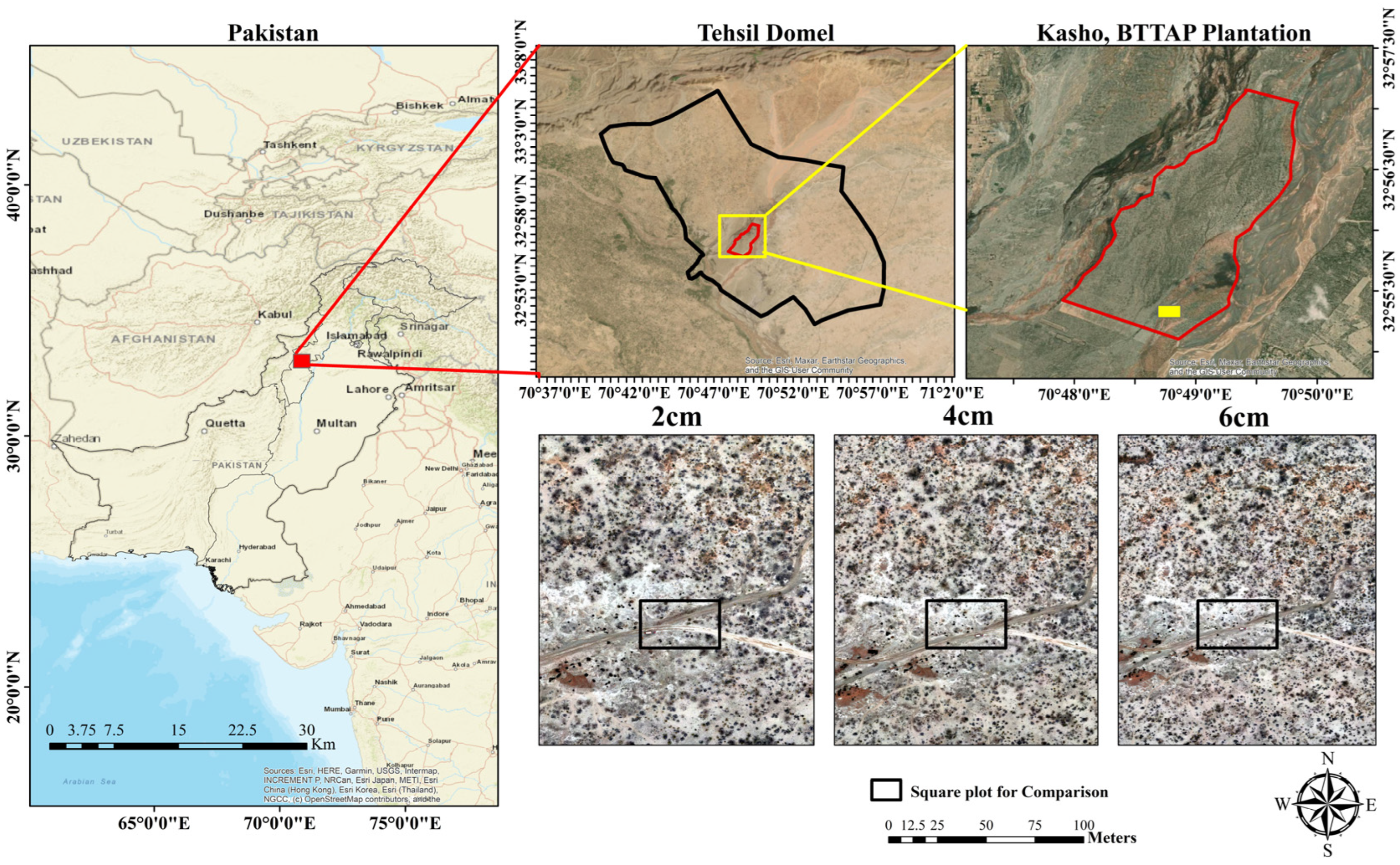
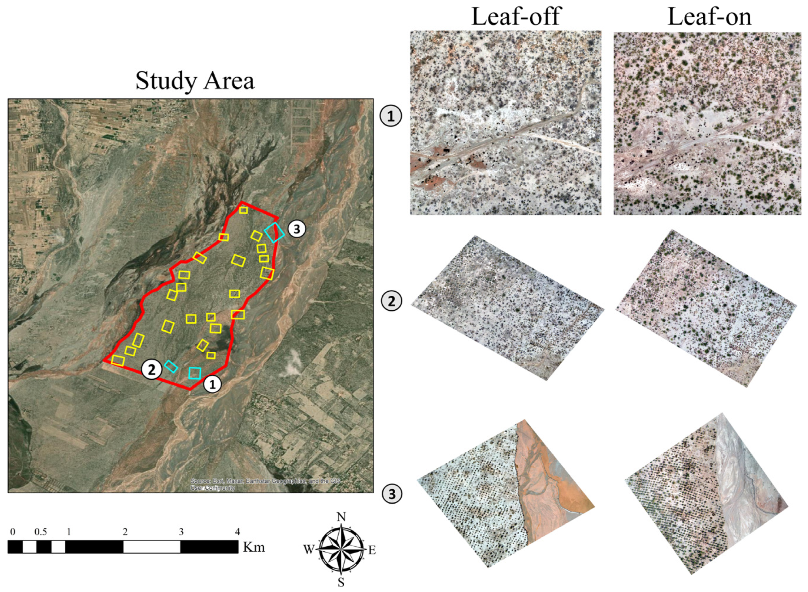
2.1. Study Area

The study was conducted in the Kasho area of Tehsil Domel, District Bannu, Khyber Pakhtunkhwa (KP), Pakistan, as part of the Billion Tree Plantation Initiative launched by the KP government in 2014 to promote sustainable forest development and combat desertification. The study area spans roughly 534 hectares, with the elevation ranging from 306 to 323 m above sea level across the sample plots, located at the coordinates 33°06′6.14″N, 70°50′45.92″E (Figure 1). This region experiences four distinct seasons, with the study focusing on two key periods: winter (mid-November to the end of March) and summer (May to September) [22]. The climate during summer is characterized by an average daily high temperature exceeding 35 °C, while in winter, it typically remains below 22 °C [23].

The natural vegetation in the area is dominated by herbaceous species such as Ammophilia arenaria and Juncus acutus, along with the shrub species Prosopis juliflora. Artificial plantations, including those containing Eucalyptus camaldulensis, Acacia nilotica, Acacia modesta, and Acacia farnesiana, are also prevalent. The study specifically focused on three sample plots, which included both natural species (Ammophilia arenaria, Juncus acutus, and Prosopis juliflora) and artificial plantations where Eucalyptus camaldulensis was the most dominant exotic species, which has a tree height range of 1–6 m.

2.2. Data Collection

The RGB UAV used for this study was the DJI Mavic Air 2, a mid-range drone with advanced features. It integrates a foldable, portable design with a sophisticated camera system, including a 3-axis gimbal and a 1/2″ Complementary Metal-Oxide-Semiconductor (CMOS) sensor (DJI-Innovations Inc., Shenzhen, China). This setup enables the capture of 8 K hyperlapse footage, time-lapse footage, 4K60 video, 240 fps slow-motion 1080 p video, and 48 MP still images. The DJI Mavic Air 2 has a lens with a focal length of 4.5 mm and a sensor size of 6.4 mm × 4.8 mm, facilitating precise vegetation mapping. Two UAV missions were conducted to evaluate the capabilities of the consumer-grade RGB UAV for precise vegetation mapping using multi-temporal and multi-resolution imagery. The first mission was conducted in late winter (8–11 March 2024), and the second in summer (29 June–1 July 2024). Both missions were scheduled between 9 AM and 4 PM local time to ensure consistent lighting conditions. The atmospheric conditions featured bright, sunny weather with negligible wind, providing optimal field visibility. Flights were conducted at three altitudes (60, 120, and 180 m), achieving spatial resolutions of 2, 4, and 6 cm, respectively. This multi-altitude approach aimed to capture imagery at varying spatial resolutions, assess the variability in vegetation mapping precision, and identify the most cost-effective resolution for RGB UAV imaging.

The flight parameters included an 80% front overlap and a 70% side overlap. The UAV operated at a maximum speed of 4.4 m/s to prevent data gaps, ensuring accurate and complete coverage of the plots.

Leaf-Off and Leaf-On Data Collection

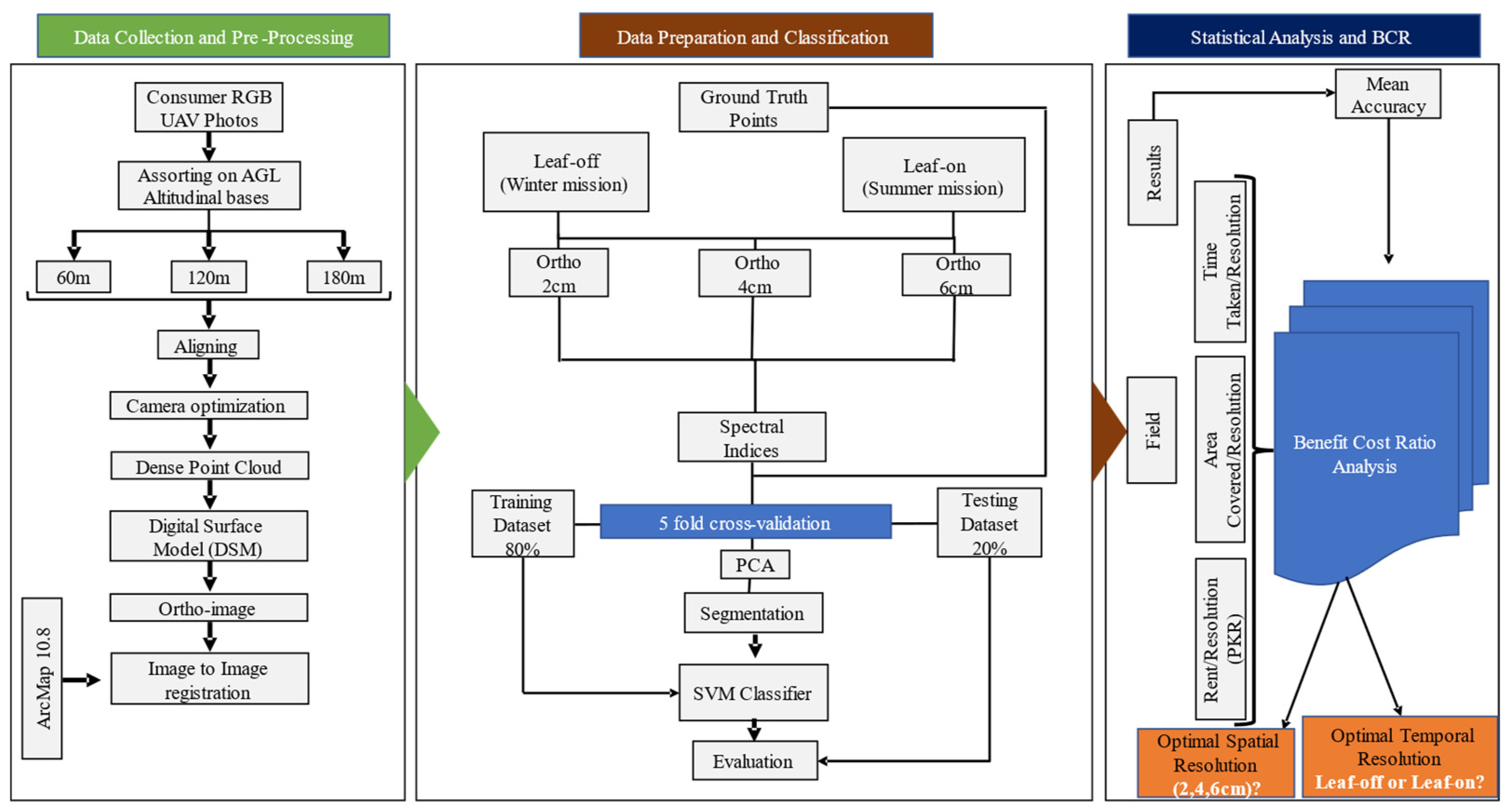
In precision forestry, using RGB UAVs for multi-temporal vegetation mapping can provide critical insights into forest structure and health. Leaf-off imagery, captured in late winter (March), enhances ground feature visibility, such as soil and understory vegetation, by reducing foliage obstruction. This is particularly useful for early-stage afforestation monitoring, enabling accurate assessment of the tree spacing, terrain, and soil conditions. Leaf-on imagery, taken during peak growth (July), captures canopy development and biomass, making it essential for evaluating vegetation health. The green band’s reflectance aids in monitoring the chlorophyll content and plant vigor. Combining leaf-off and leaf-on data provides a comprehensive view of the structural and phenological changes, optimizing the vegetation indices and improving the accuracy of afforestation evaluations and mapping (Figure 2).

2.3. Method

2.3.1. Orthoimage Generation

Pre-processing was performed using Agisoft Metashape Professional 2.1.0 and ArcMap 10.8. The UAV images were imported and aligned through key point detection, generating tie points. A dense point cloud was created using the ultra-high-quality function, producing a digital surface model (DSM) and a high-resolution orthophoto. To ensure accurate georeferencing of the images, GPS data were collected using a Garmin 64s GPS (horizontal accuracy: ~3 m). These GPS data were used to determine the land use land cover classes (vegetation and non-vegetation) and the center of each plot, providing the initial geolocation reference for both the leaf-off and leaf-on datasets. Despite the horizontal accuracy of the GPS being relatively large (~3 m), the relative alignment between the leaf-off and leaf-on orthomosaics was prioritized. This was achieved by carefully identifying and aligning the same GCPs in overlapping UAV images from both campaigns, ensuring pixel-level alignment of invariant features (such as the plot center and non-vegetation structures). The focus on relative alignment allowed for sub-pixel accuracy between the multi-temporal datasets despite some absolute geolocation discrepancies due to GPS limitations. Subsequently, the orthophoto was imported into ArcMap 10.8, where image-to-image georeferencing was performed. This process aligned the orthophotos (leaf-off and leaf-on), ensuring improved geometric accuracy. The alignment was enhanced by applying a 1st-order polynomial function, and the co-registration achieved an average RMSE of 0.01 m per plot, demonstrating high accuracy. Additionally, to maintain consistency between the datasets, the same mission planning protocol was applied for both the leaf-off and leaf-on UAV flights. This approach ensured that the number of images per resolution remained the same for both flights, further aiding the georeferencing process. The coordinate reference system used was UTM Zone 42N.

2.3.2. Feature Preparation and Principal Component Analysis (PCA) for Effective Model Training

Vegetation indices (VIs) are crucial for monitoring vegetation health, density, and growth patterns by highlighting spectral variations across the red, green, and blue (RGB) spectrum [24,25]. In this study, nine VIs were computed using ArcPy 3.1.5 and NumPy 2.0.2 for efficient geospatial data handling and pixel-based calculations. These indices, adapted from [26], were synthesized from established sources to provide a robust framework for assessing vegetation characteristics, such as the Leaf Area Index. ArcPy was used to manage raster data geospatial properties, enabling the loading of composite rasters and extraction of individual bands (red, green, and blue). The raster bands were converted to NumPy arrays for rapid pixel-wise computations of the VIs through mathematical operations (

Table 1. Vegetation indices calculated for this study.

Index	Formula	Reference
Red chromatic coordinate (RCC)	R/(R + G + B)	[24]
Green chromatic coordinate (GCC)	G/(R + G + B)	[24]
Blue chromatic coordinate (BCC)	B/(R + G + B)	[24]
Normalized difference index (NDI)	(RCC-GCC)/(RCC + GCC + 0.01)	[25]
Green leaf index (GLI)	(2 * R-G-B)/(2 * R + G + B)	[30]
Kawashima index (IKAW)	(R-B)/(R + B)	[24]
Mean of RGB bands (MRGB)	(R + G + B)/3	[31]
Excess green vegetation index (EXG)	(2 * RCC – GCC − BCC)	[25]
Visible atmospherically resistance index (VARI)	(G-R)/(G + R − B)	[32]

). The calculated indices were then converted back to a raster format using ArcPy, preserving the original geospatial extent and resolution. This approach combines ArcPy’s geospatial capabilities with NumPy’s computational efficiency, creating an automated workflow for VI calculations. Principal Component Analysis (PCA) was applied to reduce dataset dimensionality [27] and streamline the inputs for the SVM classifier. The PCA was used to integrate the spectral information from the VIs into fewer components while retaining most of the data variance, reducing computational complexity and improving classification performance [28]. By transforming multiple VIs into a composite image, PCA facilitates the integration of diverse vegetation features into a unified dataset, enhancing the efficiency and accuracy of the machine learning (ML) classification [29].

A SVM classifier categorized the vegetation and two non-vegetation classes, leveraging its ability to maximize separation in a high-dimensional space. It trains a model to position a hyperplane between data points, maximizing the margin. Specifically, we used the Radial Basis Function (RBF) kernel, which is a commonly applied default choice for SVM in remote sensing applications. The critical default parameter values used in this study were as follows:

• Kernel: RBF;
• C: 1.0 (the default value in Scikit-learn, representing the penalty parameter for misclassification);
• Gamma: ‘scale’ (the default value in Scikit-learn, which is 1/(n_features * X.var()), where n_feature = 3(RGB) + 1(PCA), while X.var() represents the variance of a given independent variable).

This study employed a 5-fold cross-validation strategy for model robustness and generalizability. The dataset was split into training and validation sets for each fold, using a composite image from UAV-acquired RGB and PCA data, which was crucial for precise classification. The SVM algorithm seeks to learn the optimal hyperplane, defined mathematically by minimizing the following objective function:

$${min}_{w,b }{\displaystyle \frac{1}{2}} {\parallel \mathrm{w}\parallel }^2$$

(1)

provided that,

$$yi\left(W^{T}Xi+b\right)\ge 1 \forall \mathrm{I}$$

(2)

where

• W: Represents the weight vector, which defines the orientation of the hyperplane in the feature space.
• b: Refers to the bias term, which adjusts the position of the hyperplane relative to the origin, allowing it to be shifted.
• Xi: The feature vector that includes both RGB ortho and PCA data, providing the input features for classification.
• Yi: Denotes the class label for each data point, representing the category or class to which the data point belongs.

After cross-validation, a final SVM model was trained with the entire dataset to generate the most accurate hyperplane for classification. This model was applied to the full composite image, producing a raster output that distinguished various classes in the RGB UAV imagery (Figure 3). SVM’s capability to handle high-dimensional, multi-source datasets, along with precise pixel-based image analysis, underscores its utility in remote sensing for detailed vegetation mapping.

2.3.3. Training and Validation

This study selected three sample plots that covered all the vegetation classes, and contain water and barren land. A stratified sampling approach was used to address the landscape’s spatial heterogeneity since a single plot was insufficient for characterization. High-resolution orthoimages from a consumer-grade RGB UAV facilitated the accurate delineation of polygons for six land cover classes. Ground control points (GCPs) ensured geospatial accuracy for the classifications [15]. Training samples were extracted to balance representation across all classes, mitigating class imbalances and enhancing the classification model’s robustness [26]. The distribution of training samples per plot (

Table 2. Distribution of training samples across vegetation classes in each sample plot.

Plot ID	EC	AA	PJ	JA	BL	W	Total
1	×	50	50	50	50	50	250
2	×	30	30	×	30	×	90
3	40	40	40	×	40	40	200

) ensured the representation of all land cover classes: EC (Eucalyptus camaldulensis), AA (Ammophilia arenaria), PJ (Prosopis juliflora), JA (Juncus acutus), BL (barren land), and W (water), even in sparsely vegetated areas.

Each sample plot was independently processed at different spatial resolutions using a classification model to evaluate the accuracy and compatibility of the UAV-based vegetation mapping across various spatial contexts. The use of multi-resolution and multi-temporal UAV data enabled a comprehensive assessment of the UAV’s capabilities for precise vegetation mapping [33].

2.3.4. Entropy Analysis for Information Gain and Loss Assessment

Entropy was employed to assess the information richness and spatial variability under the different UAV spatial and temporal resolutions, as it effectively quantifies the complexity and heterogeneity within spatial data. By measuring entropy, we can capture the variation pixel values: higher entropy indicates a complex, information-rich landscape, while lower entropy suggests uniformity with potentially lower information content. This metric is essential for determining the resolution that best balances detail with data efficiency, avoiding unnecessary redundancy [34].

Shannon entropy was specifically selected due to its widespread application in spatial analysis and remote sensing, where it quantifies uncertainty within pixel value distributions, making it suitable for comparing information densities [35,36]. It allows for a systematic examination of landscape variability, capturing the complexity of vegetation and land cover features. To implement this approach, we applied a moving window method, dividing the orthoimages into 700 × 700-pixel patches. Entropy was calculated for each patch using Shannon’s formula, and the mean entropy was computed:

$$H\left(X\right)=-\sum _{i=1}^{n}p \left(x_i\right){\log }_2\left(p\left(x_i\right)\right)$$

(3)

where

• H(X) represents the entropy of a patch;
• $p\left(x_i\right)$ is the probability of occurrence of pixel value $x_i$ within that patch.

After calculating the entropy for all patches, we computed the mean entropy across the patches for each resolution to capture the average information richness and variability within the image. We applied incremental (pairwise) entropy gain/loss values to conduct a stepwise comparison across resolutions, capturing nuanced changes in the information content as the resolution progressively coarsens (e.g., 2 to 4 cm, and 4 to 6 cm). This examination of information gain/loss provided insights into the information density retained at each spatial scale, ultimately guiding the selection of the optimal resolutions for UAV-based vegetation mapping.

3. Results

3.1. Impact of Resolution and Seasonal Conditions on Classification Accuracy and Variability

The classification performance varied depending on the resolution and season (

Table 3. Descriptive analysis of classification metrics at different resolutions and seasonal conditions for Plots 1, 2, and 3.

Resolution (cm)	Mission	Mean Accuracy	SD	Range	CV (%)	Plot Number
2	Leaf-off	0.958	0.007	0.020	0.781	Plot 1
4	=	0.968	0.032	0.080	3.357	Plot 1
6	=	0.964	0.015	0.040	1.553	Plot 1
2	Leaf-on	0.968	0.032	0.070	3.293	Plot 1
4	=	0.984	0.015	0.040	1.521	Plot 1
6	=	0.97	0.020	0.050	2.062	Plot 1
2	Leaf-off	0.964	0.029	0.060	3.049	Plot 2
4	=	0.932	0.041	0.110	4.366	Plot 2
6	=	0.912	0.044	0.110	4.825	Plot 2
2	Leaf-on	0.988	0.024	0.060	2.429	Plot 2
4	=	1	0.000	0.000	0.000	Plot 2
6	=	0.976	0.029	0.060	3.012	Plot 2
2	Leaf-off	0.884	0.036	0.100	4.085	Plot 3
4	=	0.884	0.041	0.100	4.614	Plot 3
6	=	0.906	0.023	0.060	2.574	Plot 3
2	Leaf-on	0.914	0.037	0.100	4.070	Plot 3
4	=	0.932	0.041	0.110	4.366	Plot 3
6	=	0.918	0.012	0.030	1.270	Plot 3

). In Plot 1, the leaf-off conditions showed a high mean accuracy across all resolutions (2, 4, and 6 cm), but the 4 cm resolution exhibited notable variability with a higher standard deviation and coefficient of variation (CV). In contrast, the leaf-on conditions enhanced accuracy, particularly at a resolution of 4 cm, and improved stability, with lower CV and range values. In Plot 2, the leaf-off conditions produced higher variability at the 4 and 6 cm resolutions, as shown by the increased CV and range. During the leaf-on period, the accuracy significantly improved, with the 4 cm resolution achieving perfect accuracy and zero variability. For Plot 3, the leaf-off conditions resulted in moderate accuracy, with variability peaking at the 2 and 4 cm resolutions, as indicated by the higher CV. The 6 cm classification was more stable. Under leaf-on conditions, the accuracy increased across all resolutions, with the 6 cm resolution showing the most stability and the lowest CV.

Overall, the results highlighted the variability in classification performance based on the resolution and vegetation conditions, confirming that leaf-on periods yield more consistent and accurate outcomes.

3.2. Resolution Impact on Area Coverage and Time Efficiency

The analysis of area coverage and efficiency revealed an inverse relationship between resolution and mission duration. As the resolution coarsened from 2 to 6 cm, the mission time—comprising the flight, orthomosaic generation, and classification time —decreased significantly. The 6 cm resolution achieved the highest efficiency, covering more area per unit of time. In contrast, the 2 and 4 cm resolutions required longer missions with less area covered per minute, reflecting the need for higher data precision and processing demands associated with fine resolutions. These findings highlight the trade-offs between time demands and spatial coverage in UAV remote sensing (Figure 4).

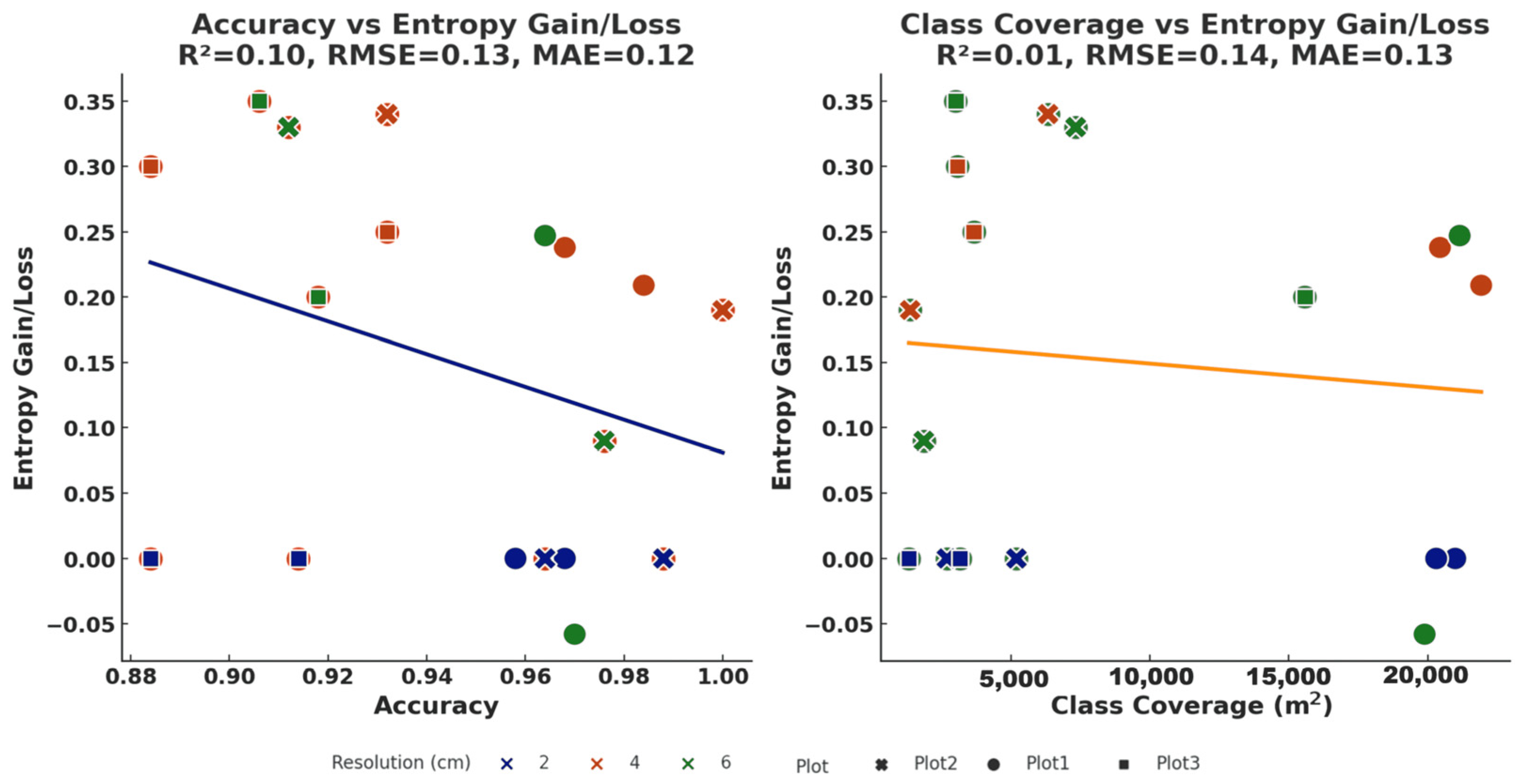
3.3. Entropy and Information Gain/Loss Across Spatial and Temporal Resolutions

The entropy analysis for the different resolutions (2, 4, and 6 cm) and seasonal conditions revealed significant differences in information capture, illustrating how resolution interacts with vegetation states (

Table 4. Summary of entropy statistics and information gain/loss across different resolutions for leaf-off and leaf-on conditions in each plot.

Plot 1
Resolution (cm)	Moving Windows	Mission	Min	Max	Mean	SD	Entropy Gain/Loss
2	25	Leaf-off	6.308	7.537	6.653	0.384	Base
4	=	=	6.232	7.511	6.891	0.478	0.238
6	=	=	6.352	7.464	7.138	0.347	0.247
2	=	Leaf-on	6.175	7.622	6.818	0.468	Base
4	=	=	6.234	7.621	7.027	0.462	0.209
6	=	=	6.370	7.566	6.970	0.398	−0.057
Plot 2
Resolution (cm)	Moving Windows	Mission	Min	Max	Mean	SD	Entropy Gain/Loss
2	42	Leaf-off	2.766	3.238	3.055	0.131	Base
4	=	=	2.611	3.232	3.002	0.164	−0.053
6	=	=	2.352	3.779	3.014	0.281	0.012
2	=	Leaf-on	2.756	3.428	3.120	0.174	Base
4	=	=	2.588	4.006	3.034	0.235	−0.086
6	=	=	2.513	4.009	3.158	0.404	0.124
Plot 3
Resolution (cm)	Moving Windows	Mission	Min	Max	Mean	SD	Entropy Gain/Loss
2	34	Leaf-off	1.390	3.855	3.168	0.651	Base
4	=	=	1.302	3.824	3.127	0.651	−0.041
6	=	=	1.276	3.825	3.126	0.633	−0.001
2	=	Leaf-on	1.881	3.606	3.001	0.511	Base
4	=	=	1.927	3.457	2.898	0.472	−0.103
6	=	=	2.163	3.422	2.941	0.371	0.043

). In Plot 1, during leaf-off conditions, the entropy gradually increased as the resolution coarsened, indicating better detection of landscape heterogeneity. However, during leaf-on conditions, the entropy slightly decreased at a resolution of 6 cm, suggesting limited additional information due to dense canopy cover. In Plot 2, under leaf-off conditions, the entropy initially decreased as the resolution coarsened from 2 to 4 cm, followed by a slight increase at 6 cm, indicating subtle shifts in spatial complexity. In contrast, during leaf-on conditions, the entropy generally declined as the resolution changed from 2 to 4 cm, with minimal gains at 6 cm, suggesting limited additional information capture at coarser resolutions due to the dense canopy cover. In Plot 3, under leaf-off conditions, the entropy slightly decreased as resolution coarsened from 2 to 4 cm and remained nearly stable at 6 cm, indicating minimal changes in the variability in structural detection. During leaf-on conditions, the entropy generally declined from a resolution of 2 to 4 cm, followed by a minor gain at 6 cm, suggesting that the dense vegetation limited the advantages of coarser resolutions, with only slight increases in information capture. These trends emphasize the need for careful resolution selection, balancing the landscape’s seasonal state and mapping objectives to optimize the resolution and information gain.

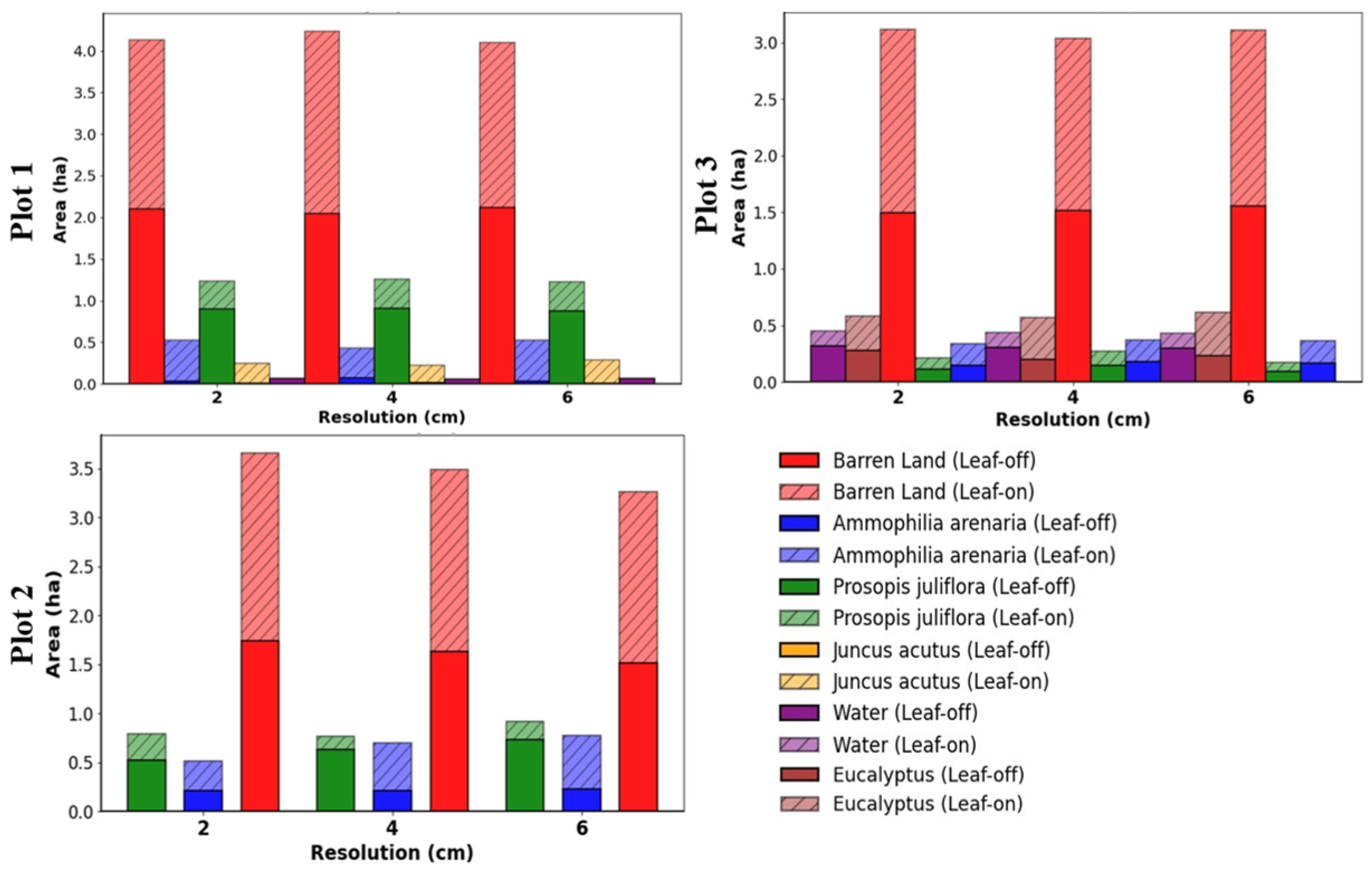
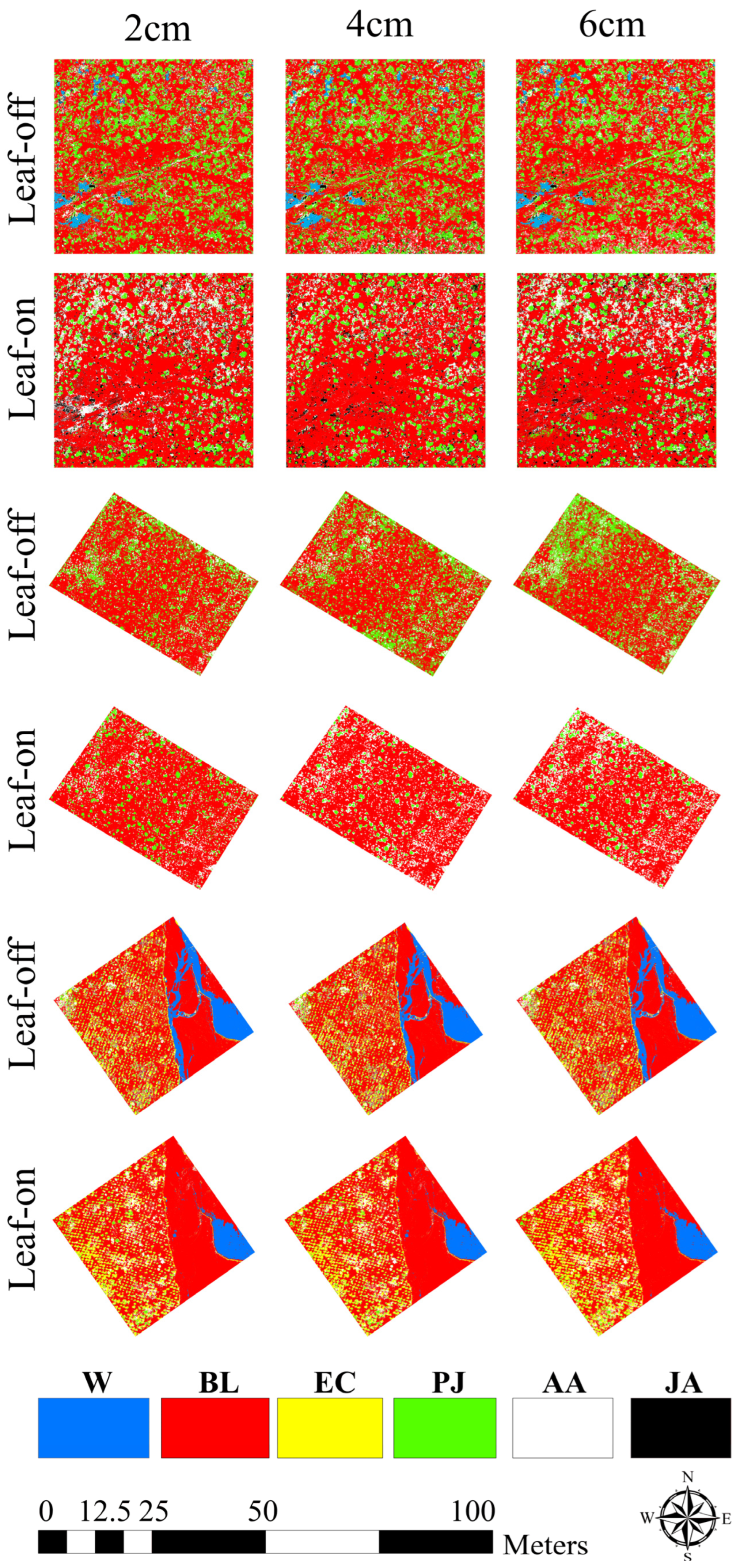
3.4. Spatial Distribution of Vegetation Classes and Area Coverage at Each Resolution

The results reveal distinct spatial and seasonal variations among the vegetation classes, with significant differences between plots and during leaf-off and leaf-on periods. Each plot had unique compositions, with some classes absent in certain areas (Figure 5). For example, water was present in Plot 1 and Plot 3 during the leaf-off season but absent in Plot 1 during the leaf-on season, with a significant decrease in Plot 3. This seasonal reduction in water affects classification accuracy and ecological dynamics. Barren land remained stable across all resolutions and seasons, while Eucalyptus camaldulensis in Plot 3 and Juncus acutus in Plot 1 were plot-specific yet seasonally stable. A challenge in winter was distinguishing between Ammophilia arenaria and Prosopis juliflora due to their high spectral similarity, leading to misclassification in mixed vegetation areas, especially at coarser resolutions. However, the increased vegetation density and chlorophyll content improved classification precision during leaf-on periods. Overall, the leaf-on period resulted in greater vegetation coverage in all plots, while barren land remained unchanged. These findings underscore the need to consider resolution and seasonal factors for effective vegetation classification in heterogeneous landscapes prone to spectral confusion (Figure 6).

3.5. Resolution and Seasonal Effects on Information Dynamics, Accuracy, and Vegetation Coverage

In Figure 7, the first scatter plot compares the accuracy and entropy gain/loss, which had a weak positive correlation (R = 0.10). Despite resolution changes (2 to 6 cm), the entropy variations had a minimal impact on accuracy, which remained consistently high. The low RMSE and MAE values confirmed the classifier’s robustness against entropy changes. This highlights that coarser resolutions can maintain reliable accuracy, balancing precision and computational efficiency for large-scale vegetation mapping. The second scatter plot examines the class coverage and entropy gain/loss, revealing no significant correlation (R = 0.01). The flat trend line indicates that the vegetation class size had little influence on information gain/loss. This weak link suggests that resolution, not class area, drove the information dynamics. Coarser resolutions thus remain practical for large-scale mapping, ensuring computational efficiency without sacrificing accuracy.

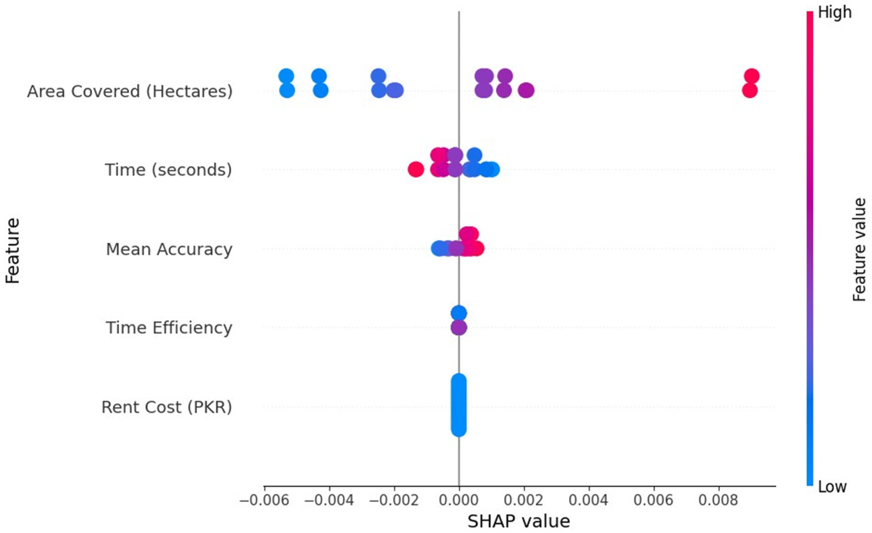
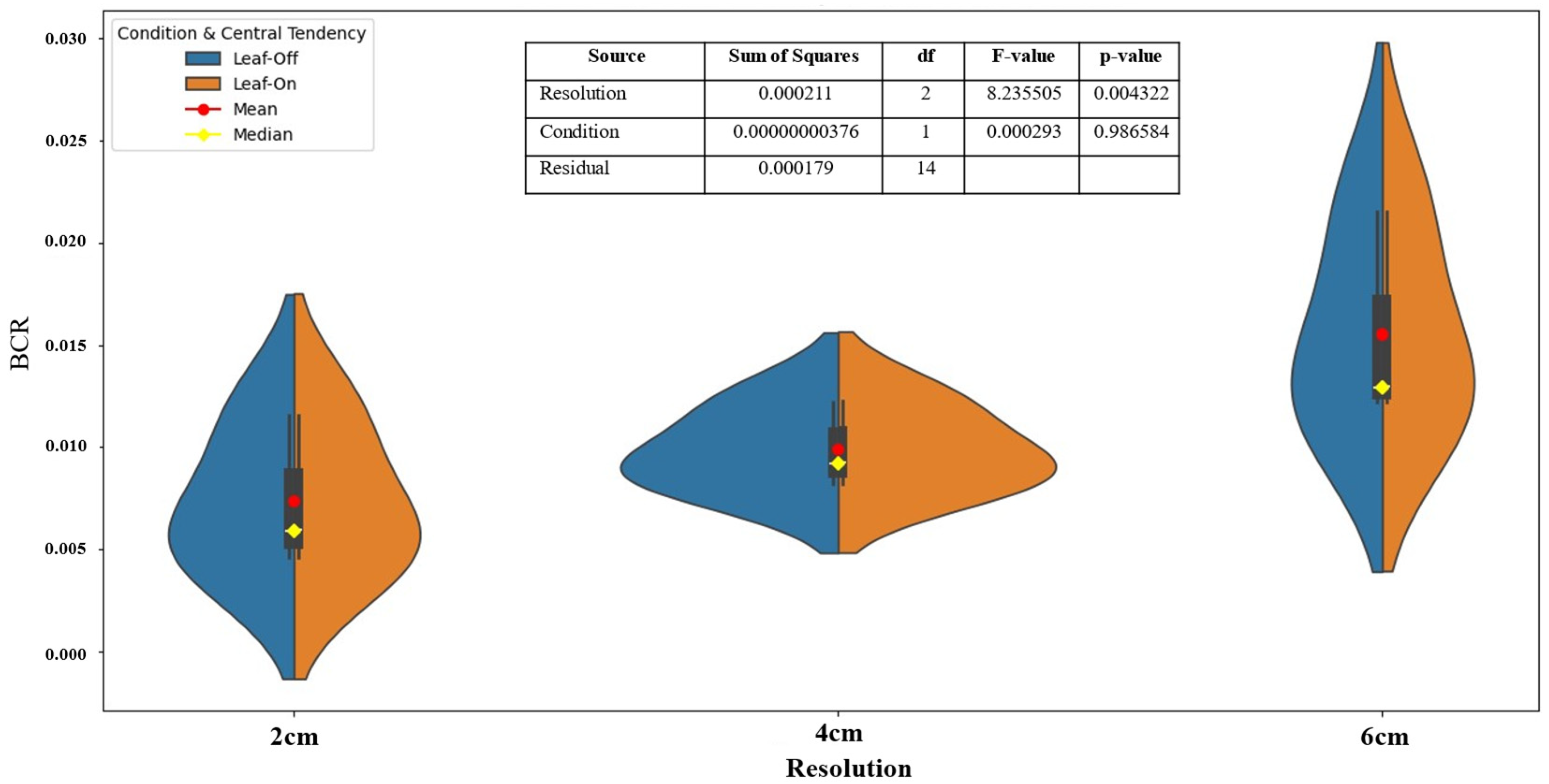
3.6. Optimizing Resolution and Mission Selection for Benefit–Cost Ratio Efficiency

The SHAP-derived feature importance analysis (Figure 8) highlighted the relative influence of key factors like area coverage, time efficiency, and classification accuracy on the BCR in UAV-based vegetation mapping. Area coverage was the most influential factor, emphasizing the need to maximize the spatial coverage for an optimal BCR, especially in large-scale ecological monitoring. Time and accuracy also contributed significantly, underscoring the importance of balancing operational duration with classification precision to enhance cost-effectiveness and reliability. This analysis provides insights for selecting parameters that optimize trade-offs between spatial extent, time, and accuracy, which is crucial for efficient large-scale vegetation monitoring.

The BCR analysis showed the 6 cm resolution’s clear advantage for UAV-based vegetation mapping (Figure 9). It consistently outperformed the others, achieving the highest BCR values in all the plots. In Plot 3, the largest area, the 6 cm resolution demonstrated the highest efficiency, with BCR values of 0.01674 (leaf-off) and 0.01696 (leaf-on), driven by extensive spatial coverage and sufficient accuracy. This highlights that maximizing the area coverage enhances operational efficiency in broad-scale mapping. In contrast, the 2 cm and 4 cm resolutions, despite slightly higher accuracies, had lower BCRs due to their reduced area coverage and increased operational time. In Plot 1, the 2 cm resolution yielded BCRs of 0.00477 (leaf-off) and 0.00482 (leaf-on), showing diminishing returns in larger plots where area coverage is critical. The leaf-on conditions generally provided slightly higher BCRs than the leaf-off conditions, but differences between the different resolutions were minimal, indicating that temporal factors had a limited impact on the cost–benefit relationships. The 6 cm resolution effectively balanced accuracy, operational time, and area coverage, making it the most cost-effective choice regardless of season. This underscores the importance of selecting a resolution that optimizes the spatial extent and operational efficiency, particularly in large-scale ecological studies requiring reliable performance across different plot sizes and seasonal conditions without compromising accuracy.

4. Discussion

4.1. Optimal Resolution for UAV-Based Vegetation Mapping

This study aimed to identify the optimal spatial resolution for UAV-based vegetation mapping in large-scale afforestation projects. Our findings show that the 6 cm resolution struck the best balance between classification accuracy and broad spatial coverage. It achieved reasonable accuracy while outperforming the finer resolutions in spatial coverage. Studies suggest that moderate resolutions are often sufficient for accurate vegetation structure analysis. These results align with [37,38], who found that excessively high resolutions (1–2 cm) can lead to data processing challenges without significant accuracy gains, especially in large-scale ecological studies. The finer 2 cm and 4 cm resolutions, despite slightly higher accuracies, result in diminishing returns in larger plots due to their limited area coverage and increased processing time. This reinforces the conclusions by Sun et al. [39] regarding diminishing returns at higher spatial resolutions.

4.2. Cost-Efficiency and Trade-Offs Between Accuracy and Resolution

Another objective was to evaluate the cost-efficiency of consumer-grade RGB UAVs at various resolutions. The 6 cm resolution emerged as the most cost-effective option, with high BCR values of 0.01674 (leaf-off) and 0.01696 (leaf-on), making it optimal for balancing the factors contributing to the BCR for extensive ecological monitoring. These findings align with studies suggesting that advanced sensors, while offering higher accuracy, may not be practical or cost-effective for large-scale applications due to their increased operational costs and processing demands [40,41].

4.3. Temporal Effects on Classification Accuracy

Seasonal variations between the leaf-off and leaf-on conditions had minor effects on the classification accuracy at the different resolutions ( Figure 7). The leaf-on conditions resulted in a slightly higher accuracy due to the increased spectral variability of vegetation, consistent with the literature [42]. However, the 6 cm resolution performed consistently well across both seasons, demonstrating its versatility for year-round monitoring. While finer resolutions captured more detail, particularly during the leaf-on season, the 6 cm resolution remained sufficient for distinguishing key vegetation types and structures in both seasons.

4.4. Practical Implications for Large-Scale Vegetation Monitoring

Our study highlights the suitability of a resolution of 6 cm for extensive environmental monitoring projects, such as afforestation and land restoration projects. The high BCR (Figure 8) achieved at this resolution makes it ideal for large-scale projects where broad area coverage is essential. The 6 cm resolution’s highest BCR values demonstrate its practical application in scenarios with limited computational resources, without compromising classification accuracy. This aligns with studies recommending coarser resolutions for large-scale mapping to balance precision and efficiency [43], making it an ideal choice for resource-constrained monitoring.

4.5. Limitations and Future Directions

This study highlights the potential of RGB UAVs for efficient vegetation mapping but we acknowledge limitations for consideration. A key constraint was the limited availability of advanced UAV technologies due to resource constraints, restricting the study to consumer-grade RGB sensors. This impacts the depth of spectral information, as RGB sensors lack the detail of multispectral or LiDAR systems, potentially affecting the vegetation analysis in ecologically complex areas. One notable limitation of our study is that it only tested UAV-based RGB imagery at resolutions of 2, 4, and 6 cm, without evaluating the performance of coarser resolutions, such as 8 or 10 cm. Our study focused on resolutions up to 6 cm, as this range is particularly effective for capturing fine-scale features in early-stage afforestation projects. Testing resolutions beyond 6 cm (e.g., 8–10 cm) was limited by the UAV’s battery capacity, which restricted flight endurance at higher altitudes. Additionally, since the afforested trees in our study were young (e.g., seedlings and saplings), coarser resolutions risk oversimplifying their morphological characteristics, such as leaf structure or stem density. These details are crucial for accurate species identification and health assessments [44]. Additionally, refining UAV flight parameters, such as altitude, overlap, and path optimization, could enhance spatial coverage and data acquisition efficiency, reducing operational costs while maintaining data quality. Addressing these limitations and advancements could significantly strengthen UAV-based vegetation monitoring frameworks, particularly in resource-constrained regions, and provide valuable insights for sustainable, large-scale afforestation and restoration initiatives.

5. Conclusions

This study demonstrates the viability of consumer-grade RGB UAVs for large-scale vegetation mapping at a cost-efficient resolution of 6 cm. It balances key factors—spatial coverage, operational time, and classification accuracy— to achieve the highest BCRs and making it suitable for applications like afforestation and ecological restoration. While the finer resolutions (2 and 4 cm) provided more detailed data, their limited coverage and longer operational time make them impractical for large-scale applications. The 6 cm resolution offers an optimal balance between precision and efficiency, making it a practical choice for cost-effective environmental monitoring. Moreover, the affordability of consumer-grade UAVs could promote widespread adoption in areas with limited access to advanced UAV technologies. This study highlights their potential in addressing gaps in vegetation mapping, particularly in resource-limited environments. Future research should explore integrating advanced sensors (e.g., multispectral and LiDAR) or investigating coarser resolutions to maintain accuracy while addressing scalability challenges. These advancements could enhance UAV technology’s role in global environmental monitoring and conservation, providing a cost-effective, fast, and detailed alternative to traditional methods.

References

1. Food and Agriculture Organization of the United Nations. The State of the World’s Forests 2018. Forest Pathways to Sustainable Development. 2018. Available online: http://www.fao.org/3/ca0188en/ca0188en.pdf (accessed on 13 November 2024).
2. Gorte, R.W. Carbon Sequestration in Forests; DIANE Publishing: Darby, PA, USA, 2009. [Google Scholar]
3. Burrell, A.L.; Evans, J.P.; De Kauwe, M.G. Anthropogenic climate change has driven over 5 million km2 of drylands towards desertification. Nat. Commun. 2020, 11, 3853. [Google Scholar] [CrossRef]
4. Bristol-Alagbariya, E.T. UN Convention to Combat Desertification as an International Environmental Regulatory Framework for Protecting and Restoring the World’s Land towards a Safer, More Just and Sustainable Future. Int. J. Energy Environ. Res. 2023, 11, 1–32. [Google Scholar] [CrossRef]
5. Intergovernmental Panel on Climate Change. IPCC Special Report on Climate Change, Desertification, Land Degradation, Sustainable Land Management, Food Security, and Greenhouse Gas Fluxes in Terrestrial Ecosystems. In Climate Change and Land; Cambridge University Press: Cambridge, UK, 2022. [Google Scholar] [CrossRef]
6. Aziz, T. Changes in land use and ecosystem services values in Pakistan, 1950–2050. Environ. Dev. 2021, 37, 100576. [Google Scholar] [CrossRef]
7. Kamal, A.; Yingjie, M.; Ali, A. Significance of billion tree tsunami afforestation project and legal developments in forest sector of Pakistan. Int. J. Law Soc. 2019, 1, 20. [Google Scholar]
8. Rehman, J.U.; Alam, S.; Khalil, S.; Hussain, M.; Iqbal, M.; Khan, K.A.; Sabir, M.; Akhtar, A.; Raza, G.; Hussain, A.; et al. Major threats and habitat use status of Demoiselle crane (Anthropoides virgo), in district Bannu, Pakistan. Braz. J. Biol. 2021, 82, e242636. [Google Scholar] [CrossRef]
9. Çalişkan, S.; Boydak, M. Afforestation of arid and semiarid ecosystems in Turkey. Turk. J. Agric. For. 2017, 41, 317–330. [Google Scholar] [CrossRef]
10. Muñoz-Pizza, D.M.; Villada-Canela, M.; Rivera-Castañeda, P.; Reyna-Carranza, M.A.; Osornio-Vargas, A.; Martínez-Cruz, A.L. Stated benefits from air quality improvement through urban afforestation in an arid city—A contingent valuation in Mexicali, Baja California, Mexico. Urban For. Urban Green. 2020, 55, 126854. [Google Scholar] [CrossRef]
11. Che’Ya, N.N.; Dunwoody, E.; Gupta, M. Assessment of weed classification using hyperspectral reflectance and optimal multispectral UAV imagery. Agronomy 2021, 11, 1435. [Google Scholar] [CrossRef]
12. Qiao, Y.; Jiang, Y.; Zhang, C. Contribution of karst ecological restoration engineering to vegetation greening in southwest China during recent decade. Ecol. Indic. 2021, 121, 107081. [Google Scholar] [CrossRef]
13. Hu, J.; Peng, J.; Zhou, Y.; Xu, D.; Zhao, R.; Jiang, Q.; Fu, T.; Wang, F.; Shi, Z. Quantitative estimation of soil salinity using UAV-borne hyperspectral and satellite multispectral images. Remote Sens. 2019, 11, 736. [Google Scholar] [CrossRef]
14. Lu, Y.; Xue, Z.; Xia, G.-S.; Zhang, L. A survey on vision-based UAV navigation. Geo-Spat. Inf. Sci. 2018, 21, 21–32. [Google Scholar] [CrossRef]
15. Zhang, Y.; Migliavacca, M.; Penuelas, J.; Ju, W. Advances in hyperspectral remote sensing of vegetation traits and functions. Remote Sens. Environ. 2021, 252, 112121. [Google Scholar] [CrossRef]
16. Dalponte, M.; Bruzzone, L.; Gianelle, D. Fusion of hyperspectral and LIDAR remote sensing data for classification of complex forest areas. IEEE Trans. Geosci. Remote Sens. 2008, 46, 1416–1427. [Google Scholar] [CrossRef]
17. Wallace, L.; Lucieer, A.; Malenovský, Z.; Turner, D.; Vopěnka, P. Assessment of forest structure using two UAV techniques: A comparison of airborne laser scanning and structure from motion (SfM) point clouds. Forests 2016, 7, 62. [Google Scholar] [CrossRef]
18. Brede, B.; Calders, K.; Lau, A.; Raumonen, P.; Bartholomeus, H.M.; Herold, M.; Kooistra, L. Non-destructive tree volume estimation through quantitative structure modelling: Comparing UAV laser scanning with terrestrial LIDAR. Remote Sens. Environ. 2019, 233, 111355. [Google Scholar] [CrossRef]
19. Chen, X.; Sun, Y.; Qin, X.; Cai, J.; Cai, M.; Hou, X.; Yang, K.; Zhang, H. Assessing the potential of UAV for large-scale fractional vegetation cover mapping with satellite data and machine learning. Remote Sens. 2024, 16, 3587. [Google Scholar] [CrossRef]
20. Deval, K.; Joshi, P.K. Vegetation type and land cover mapping in a semi-arid heterogeneous forested wetland of India: Comparing image classification algorithms. Environ. Dev. Sustain. 2022, 24, 3947–3966. [Google Scholar] [CrossRef]
21. Ullah, S.U.; Zeb, M.; Ahmad, A.; Ullah, S.; Khan, F.; Islam, A. Monitoring the Billion Trees Afforestation Project in Khyber Pakhtunkhwa, Pakistan through remote sensing. Acadlore Trans. Geosci. 2024, 3, 89–97. [Google Scholar] [CrossRef]
22. Haq, I.U.; Mehmood, Z.; Khan, G.A.; Kainat, B.; Ahmed, B.; Shah, J.; Sami, A.; Nazar, M.S.; Xu, J.; Xiang, H. Modeling the effect of climatic conditions and topography on malaria incidence using Poisson regression: A retrospective study in Bannu, Khyber Pakhtunkhwa, Pakistan. Front. Microbiol. 2024, 14, 1303087. [Google Scholar] [CrossRef]
23. Ullah, N. Nasib Ullah. Master’s Thesis, University of Science and Technology Bannu, Bannu, Pakistan, 2021. [Google Scholar] [CrossRef]
24. Kawashima, S. An algorithm for estimating chlorophyll content in leaves using a video camera. Ann. Bot. 1998, 81, 49–54. [Google Scholar] [CrossRef]
25. Woebbecke, D.M.; Meyer, G.E.; Von Bargen, K.; Mortensen, D.A. Color indices for weed identification under various soil, residue, and lighting conditions. Trans. ASAE 1995, 38, 259–269. [Google Scholar] [CrossRef]
26. Ilniyaz, O.; Du, Q.; Shen, H.; He, W.; Feng, L.; Azadi, H.; Kurban, A.; Chen, X. Leaf area index estimation of pergola-trained vineyards in arid regions using classical and deep learning methods based on UAV-based RGB images. Comput. Electron. Agric. 2023, 207, 107723. [Google Scholar] [CrossRef]
27. Lesani, F.S.; Fotouhi Ghazvini, F.; Amirkhani, H. Smart home resident identification based on behavioral patterns using ambient sensors. Pers. Ubiquitous Comput. 2021, 25, 151–162. [Google Scholar] [CrossRef]
28. Jolliffe, I.T.; Cadima, J. Principal component analysis: A review and recent developments. Philos. Trans. R. Soc. Math. Phys. Eng. Sci. 2016, 374, 20150202. [Google Scholar] [CrossRef]
29. Shlens, J. A tutorial on principal component analysis. arXiv 2014, arXiv:1404.1100. [Google Scholar] [CrossRef]
30. Louhaichi, M.; Borman, M.M.; Johnson, D.E. Spatially located platform and aerial photography for documentation of grazing impacts on wheat. Geocarto Int. 2001, 16, 65–70. [Google Scholar] [CrossRef]
31. Ahmad, I.S.; Reid, J.F. Evaluation of colour representations for maize images. J. Agric. Eng. Res. 1996, 63, 185–195. [Google Scholar] [CrossRef]
32. Gitelson, A.A.; Kaufman, Y.J.; Stark, R.; Rundquist, D. Novel algorithms for remote estimation of vegetation fraction. Remote Sens. Environ. 2002, 80, 76–87. [Google Scholar] [CrossRef]
33. Feng, Q.; Yang, J.; Liu, Y.; Ou, C.; Zhu, D.; Niu, B.; Liu, J.; Li, B. Multi-temporal unmanned aerial vehicle remote sensing for vegetable mapping using an attention-based recurrent convolutional neural network. Remote Sens. 2020, 12, 1668. [Google Scholar] [CrossRef]
34. Shannon, C.E. A mathematical theory of communication. Bell Syst. Tech. J. 1948, 27, 379–423. [Google Scholar] [CrossRef]
35. Stoy, P.C.; Williams, M.; Spadavecchia, L.; Bell, R.A.; Prieto-Blanco, A.; Evans, J.G.; van Wijk, M.T. Using information theory to determine optimum pixel size and shape for ecological studies: Aggregating land surface characteristics in Arctic ecosystems. Ecosystems 2009, 12, 574–589. [Google Scholar] [CrossRef]
36. Altieri, L.; Cocchi, D. Entropy Measures for Environmental Data: Description, Sampling and Inference for Data with Dependence Structures; Springer Nature Singapore: Singapore, 2024. [Google Scholar] [CrossRef]
37. Turner, W.; Spector, S.; Gardiner, N.; Fladeland, M.; Sterling, E.; Steininger, M. Remote sensing for biodiversity science and conservation. Trends Ecol. Evol. 2003, 18, 306–314. [Google Scholar] [CrossRef]
38. Dandois, J.P.; Ellis, E.C. Remote sensing of vegetation structure using computer vision. Remote Sens. 2010, 2, 1157–1176. [Google Scholar] [CrossRef]
39. Sun, Z.; Wang, X.; Wang, Z.; Yang, L.; Xie, Y.; Huang, Y. UAVs as remote sensing platforms in plant ecology: Review of applications and challenges. J. Plant Ecol. 2021, 14, 1003–1023. [Google Scholar] [CrossRef]
40. Sahana, M. Conservation, Management and Monitoring of Forest Resources in India; Springer International Publishing AG: Cham, Switzerland, 2022. [Google Scholar]
41. Nex, F.; Remondino, F. UAV for 3D mapping applications: A review. Appl. Geomat. 2014, 6, 1–15. [Google Scholar] [CrossRef]
42. Shang, C.; Treitz, P.; Caspersen, J.; Jones, T. Estimation of forest structural and compositional variables using ALS data and multi-seasonal satellite imagery. Int. J. Appl. Earth Obs. Geoinf. 2019, 78, 360–371. [Google Scholar] [CrossRef]
43. Tampubolon, W.; Reinhardt, W. UAV data processing for large scale topographical mapping. Int. Arch. Photogramm. Remote Sens. Spat. Inf. Sci. 2014, XL–5, 565–572. [Google Scholar] [CrossRef]
44. Zhou, X.; Wang, H.; Chen, C.; Nagy, G.; Jancso, T.; Huang, H. Detection of growth change of young forest based on UAV RGB images at single-tree level. Forests 2023, 14, 141. [Google Scholar] [CrossRef]
Figure 1. The map shows the geographical location of the study area in the Kasho region. RGB UAV images at three resolutions have been captured for a selected sample plot—yellow, which is one of three distinct sample plots for this study—with black rectangles marking the targeted vegetation area used for comparative analysis.
Remotesensing 17 00949 g001
Figure 2. Comparison of leaf-off and leaf-on orthoimages for three sample plots (1–3), highlighting seasonal transitions in vegetation classes—from exposed soil and understory in leaf-off to dense canopy coverage in leaf-on images, where red outlines the study area boundary, yellow marks all sample plots, and light blue highlights the selected sample plots for this study.
Remotesensing 17 00949 g002
Figure 3. Workflow for precise vegetation mapping and benefit–cost ratio (BCR) analysis.
Remotesensing 17 00949 g003
Figure 4. Total time and area coverage efficiency across different resolutions, with median, and standard deviation indicated via error bars.
Remotesensing 17 00949 g004
Figure 5. Bar graphs showing the area distribution of vegetation classes across different resolutions (2, 4, and 6 cm) in leaf-on and leaf-off conditions.
Remotesensing 17 00949 g005
Figure 6. Precise mapping of vegetation and non-vegetation classes where W = water, BL = barren land, EC = Eucalyptus camaldulensis, PJ = Prosopis juliflora, AA = Ammophila arenaria, and JA = Juncus acutus.
Remotesensing 17 00949 g006
Figure 7. Pearson correlation between accuracy, class coverage, and entropy gain/loss across resolutions, where the shape of the points denotes the sample plot number, and the color of the crosses indicates the resolution of the corresponding sample plot.
Remotesensing 17 00949 g007
Figure 8. SHAP summary plot of feature contributions to BCR in UAV-based vegetation mapping.
Remotesensing 17 00949 g008
Figure 9. Effect of resolution and seasonal condition on BCR, analyzed by two-way ANOVA, highlighting a significant impact of resolution compared to the effect of condition. (α = 0.005).
Remotesensing 17 00949 g009