
Adaptive Global Dense Nested Reasoning Network into Small Target Detection in Large-Scale Hyperspectral Remote Sensing Image


Abstract
1. Introduction
- (1)
- Dense Cross-Scale Feature Aggregation U-Net: This approach breaks through the limitations of traditional U-Net’s unidirectional feature transmission by designing a high-dimensional densely nested structure, which is a variant of U-Net++. Through a cross-layer multi-path feature interaction mechanism, it enables dynamic fusion of shallow details and deep semantics. An adaptive feature weighting strategy is introduced to significantly enhance the deep feature retention capability for weak small targets, addressing the core issue of progressive feature attenuation in conventional networks.
- (2)
- Spectral–Physical Correlation Enhancement Model: A spectral–physical coupling framework is proposed, integrating biochemical parameters. By modeling the band relationships with physical constraints and incorporating an adaptive parameter fusion mechanism, this framework constructs a nonlinear correlation model between spectral responses and target biochemical attributes. It enhances the spectral distinguishability of ground objects across different sensor scenarios, effectively overcoming the interference caused by sensor parameter differences.
- (3)
- Knowledge Graph-Driven Adaptive Reasoning Framework: A graph attention network is constructed that integrates a geospatial knowledge graph, encoding prior knowledge such as environmental topology and target occurrence patterns into graph nodes. A hierarchical attention mechanism is used to achieve probabilistic reasoning of target–background relationships. This framework overcomes the semantic fragmentation bottleneck of traditional purely data-driven methods, enabling adaptive suppression of background interference and collaborative enhancement of target semantics in complex scenarios.
2. Methods
2.1. Overview
2.2. Feature Extraction Module
2.2.1. The Dense Nested Network
2.2.2. Channel and Spatial Attention Module
2.2.3. Feature Output Module
2.2.4. Convolutional Classification Module
2.3. Surface Feature Extraction Module
2.3.1. Land Surface Parameters
- (1)
- Normalized Difference Vegetation Index (NDVI) [37]
- (2)
- Leaf Area Index (LAI) [38]
- (3)
- Ratio Vegetation Index (RVI) [41]
- (4)
- Difference Vegetation Index (DVI)
- (5)
- Temperature–Vegetation Dryness Index (TDVI) [42]
2.3.2. Land Surface Classification and Feature Extraction Based on NDVI
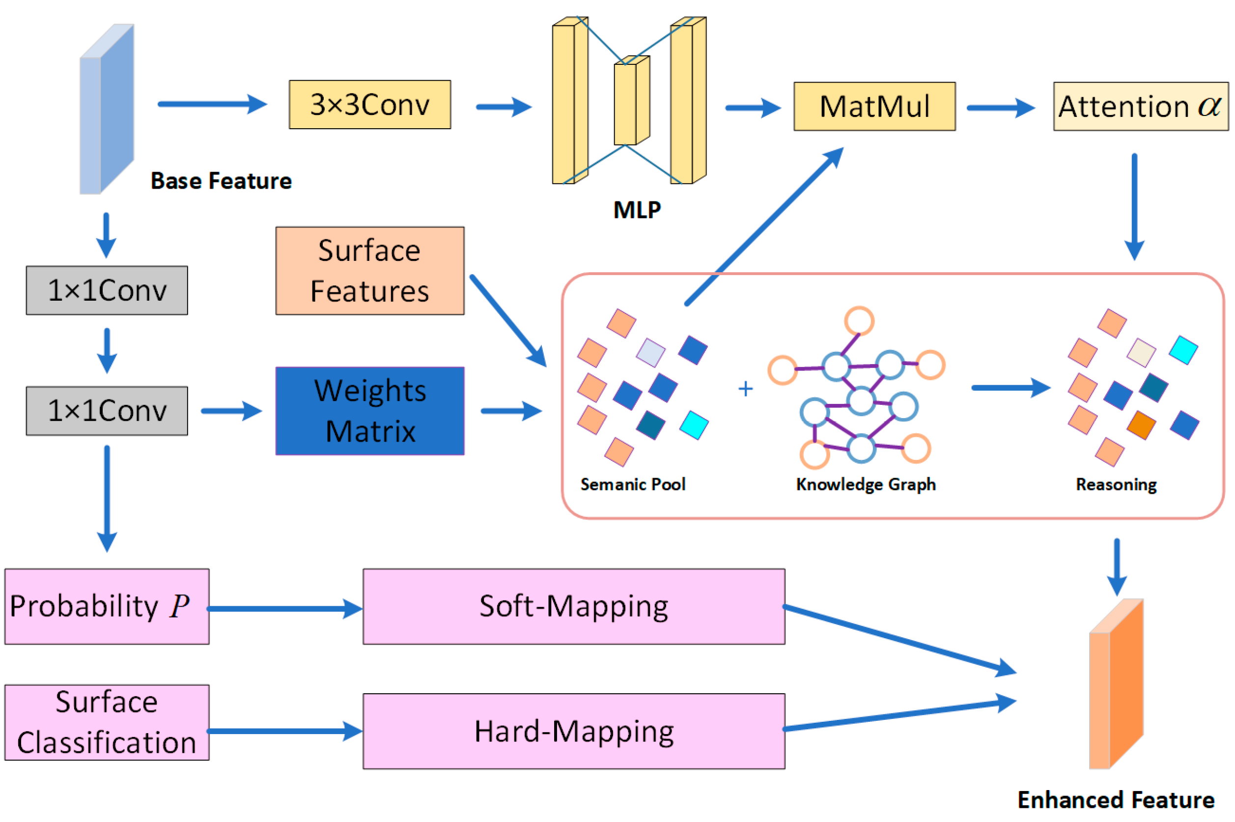
2.4. Pixel-Level Knowledge Reasoning Module
2.4.1. Knowledge Graph Construction
2.4.2. Knowledge Reasoning
2.4.3. Attention Mechanism
2.4.4. Loss Function:
3. Experiments and Results
3.1. Dataset Introduction
- (1)
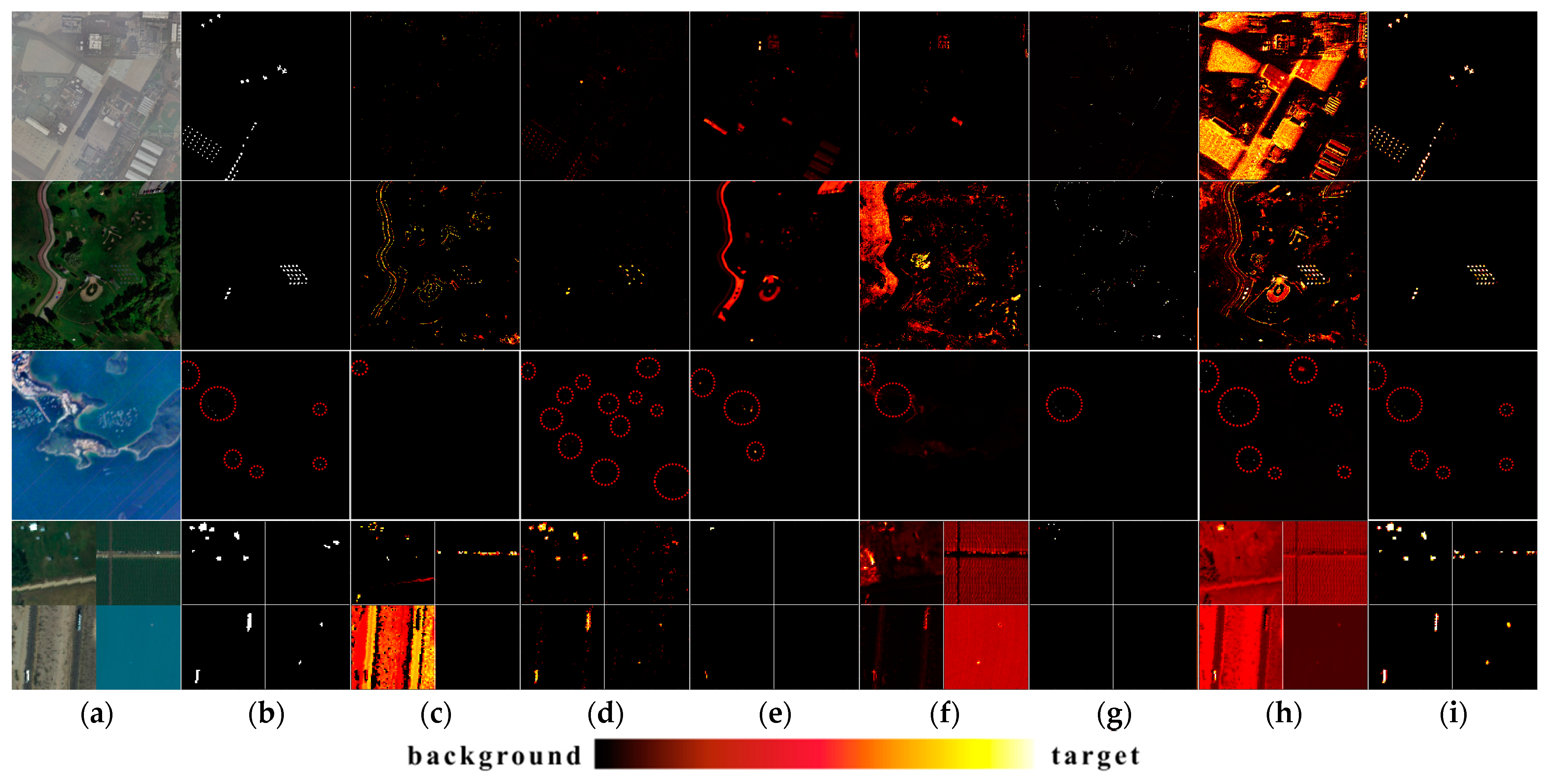
- San Diego Dataset: The San Diego dataset contains hyperspectral remote sensing images captured by the AVIRIS sensor at the United States San Diego airport. The image has a spatial resolution of 3.5 m and the size of 400 × 400 pixels. It includes 224 bands ranging from 370 to 2510 nanometers. After removing bands influenced by atmospheric effects, 203 usable bands remain. The dataset includes 1103 target pixels, covering six aircraft and other small targets of interest. These targets vary in size, ranging from a few pixels to several dozen, making it suitable for evaluating the model’s ability to detect targets of different scales. The RGB image of this dataset is shown in Figure 5a [43].
- (2)
- Mosaic Avon Dataset: The Mosaic Avon dataset is part of the “SpecTIR Hyperspectral Airborne Experiment 2012” project. It captures a section of Avon Park in New York, USA, using a push-broom sensor. The sensor collects spectral data across 360 bands, ranging from 400 to 2450 nm, where each band’s wavelength is carefully labeled. The spatial resolution of this dataset ranges from 1 to 5 m. For this study, a 256 × 256 pixels sub-region was selected, which includes large grassland areas interspersed with smaller land and road patches. The dataset contains 228 target pixels for detection [44].
- (3)
- Synthetic Dataset: The background of our synthetic dataset is derived from the TG1HRSSC hyperspectral dataset [45], collected by the Chinese Academy of Sciences Space Application Engineering and Technology Center in 2021 from the Tiangong-1 satellite. This dataset includes images across three spectral ranges: full-color (PAN), visible near-infrared (VNIR), and short-wave infrared (SWIR). It covers nine geographic categories such as urban areas, farmland, ports, and airports. In this paper, three hyperspectral images of port areas were selected. These images, sized at 256 × 256 pixels with 54 bands ranging from 400 to 1000 nm, consist of sea areas, vegetation, and urban land surfaces. The targets for this dataset were extracted from the ABU (Airport–Beach–Urban) dataset [46], which was manually curated from the AVIRIS website. The targets include aircraft, ships, and cars, which were resized, spectrally adjusted, and then randomly selected and dropped into the water and urban areas of the background dataset, creating three synthetic HSI images. Each of these images contains more than ten unique targets for detection.
- (4)
- HAD100 Dataset: The HAD100 dataset is collected by the AVIRIS sensor. The dataset is uniformly cropped into 64 × 64 image patches, with each image containing one to several small targets, with each consisting of a few to tens of pixels. The dataset includes 276 bands ranging from 400 to 2500 nm. We selected 40 images from the HAD100 dataset for training and testing, which contain multiple types of targets. We categorized the targets into four classes [47].
3.2. Experimental Details
3.2.1. Evaluation Metrics
3.2.2. Parameter Settings
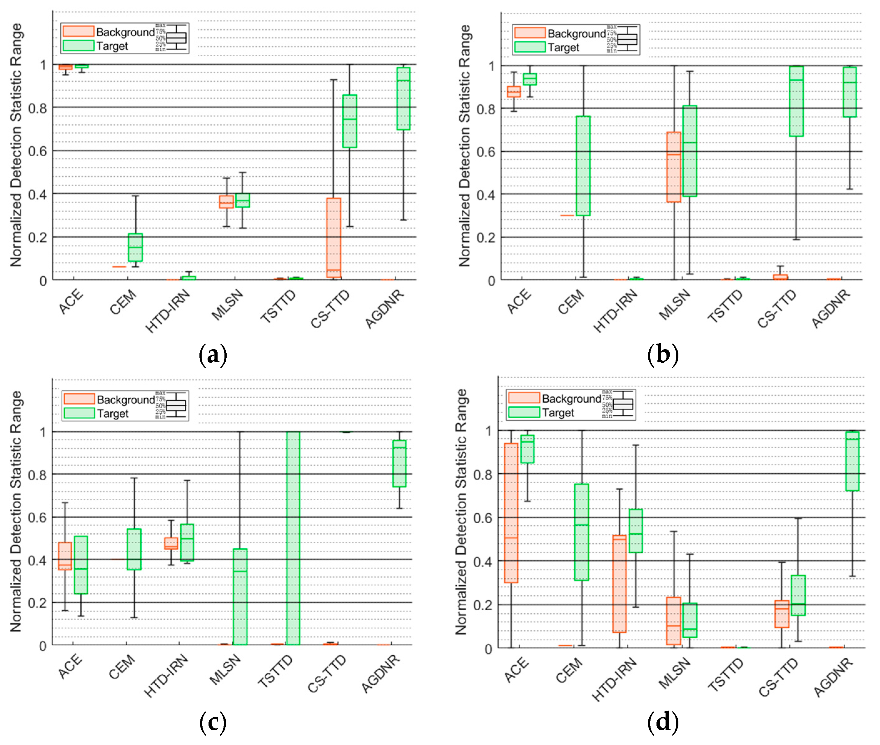
3.3. Comparison of Algorithm Performance
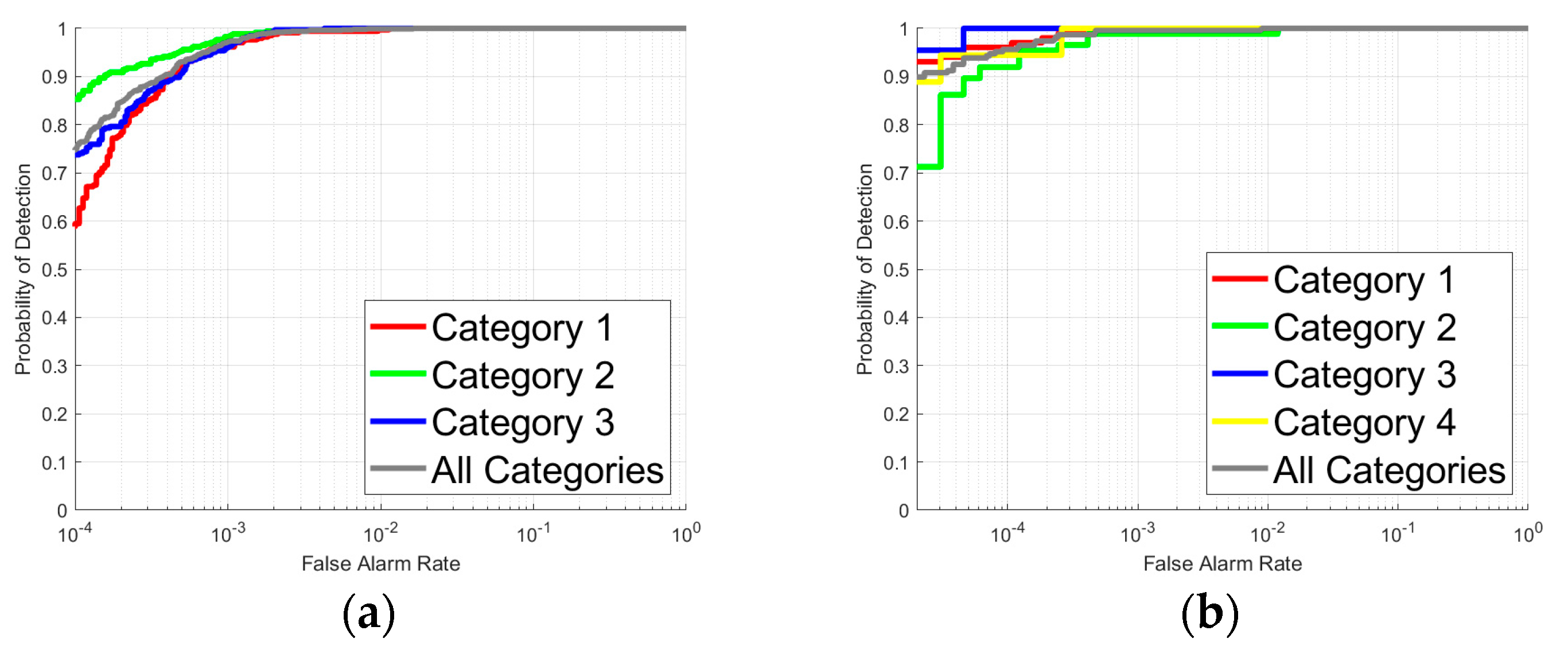
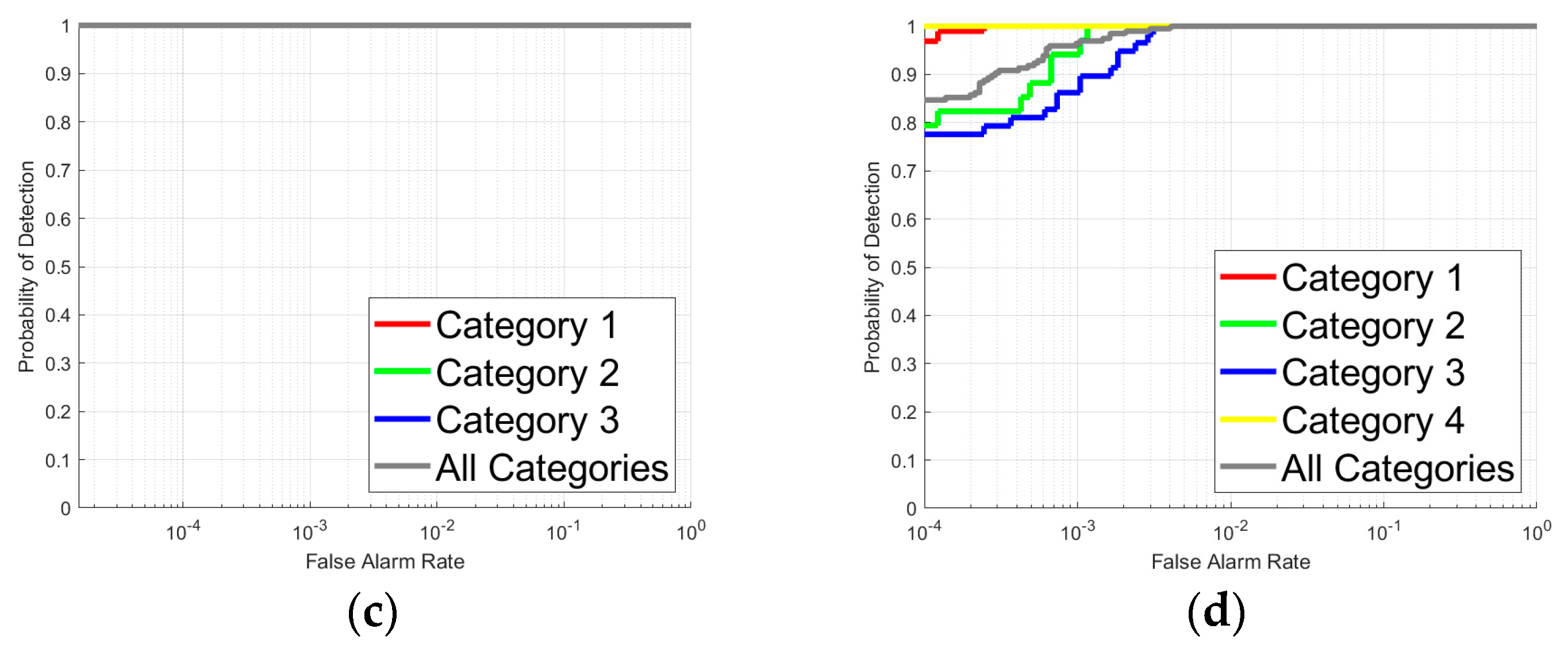
3.4. Target Type Reasoning Analysis
3.5. Ablation Experiment
3.5.1. Module Ablation
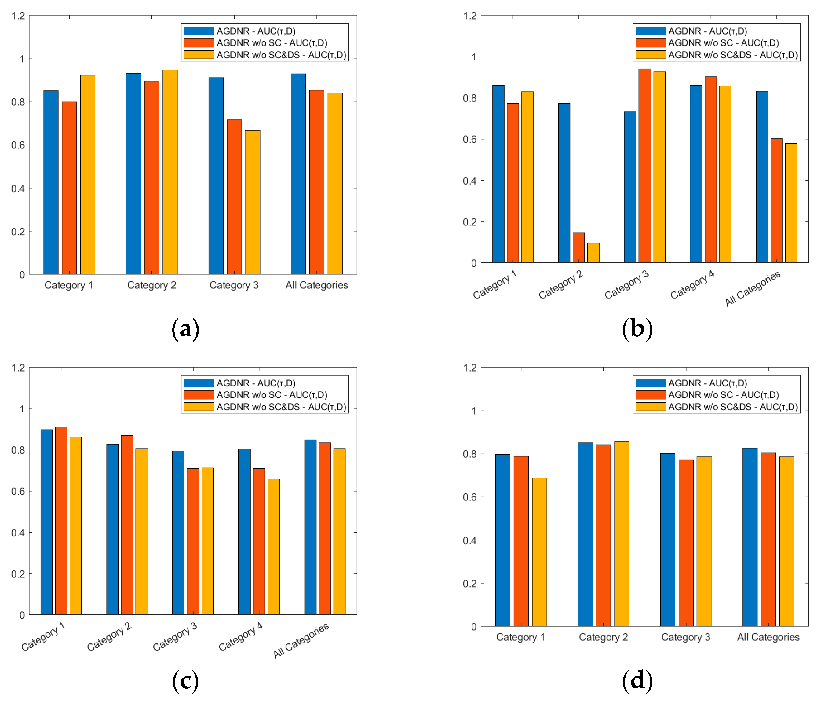
- (1)
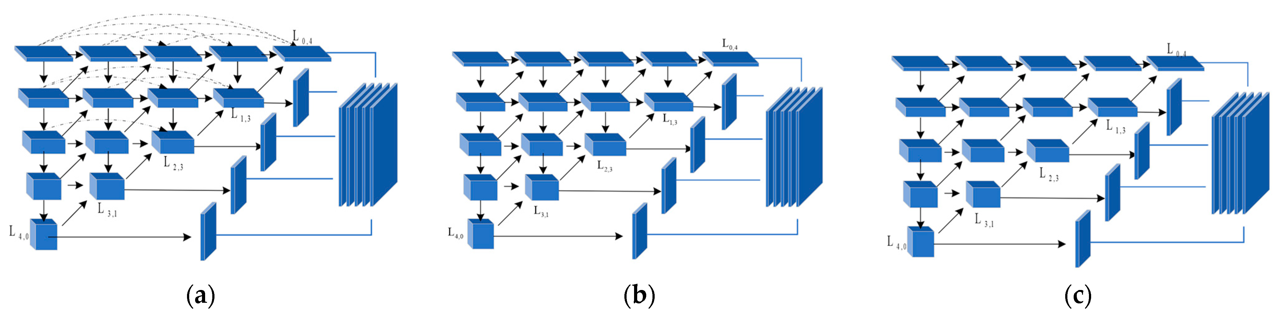
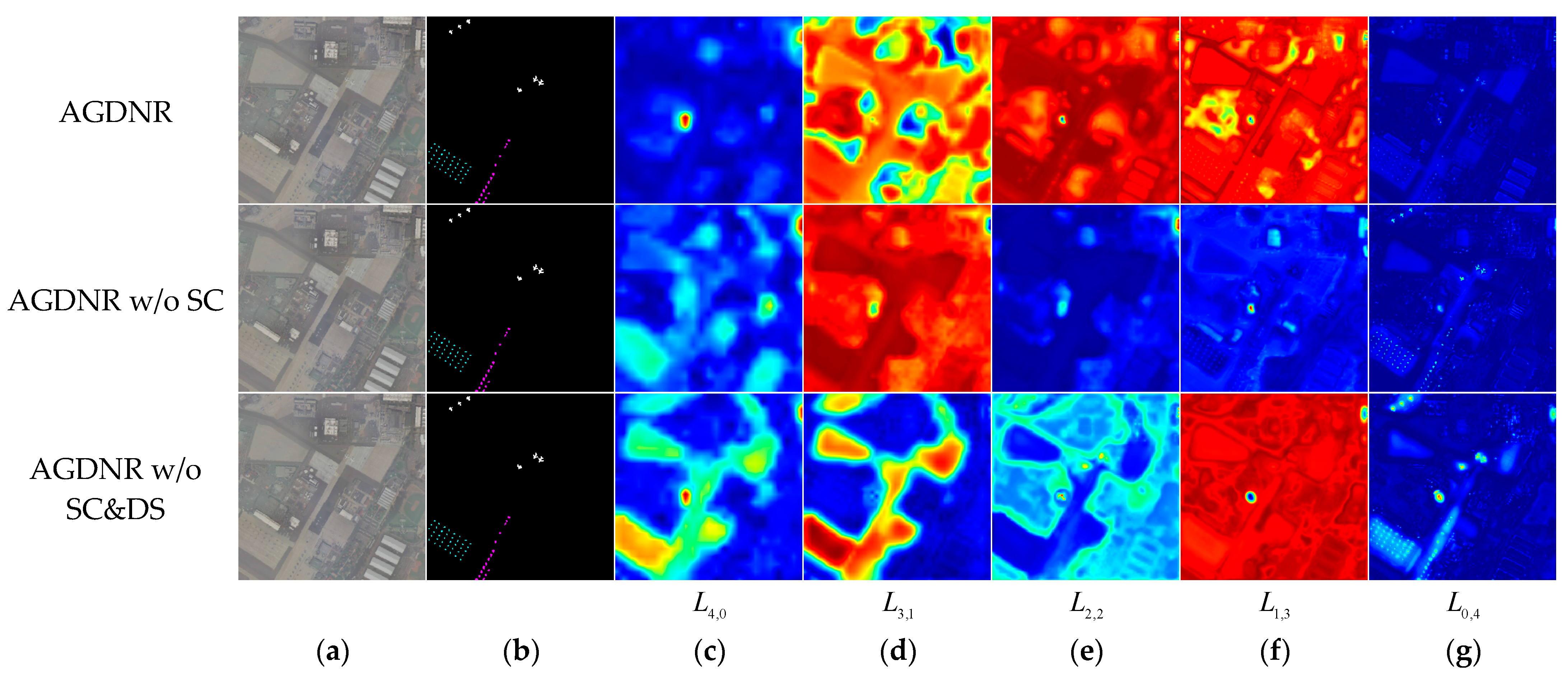
- AGDNR w/o SC: As shown in Figure 11a, the skip connections in the original model link features within the same layer, which helps to preserve the features of the preceding layers in subsequent convolutional networks. As illustrated in Figure 11b, all skip connections in the model are removed to obtain a variant.
- (2)
- AGDNR w/o SC&DS: Down-sampling layers are used to maintain the features of small targets in deep networks. As shown in Figure 11c, we remove all the down-sampling layers except for the first column to form a variant.
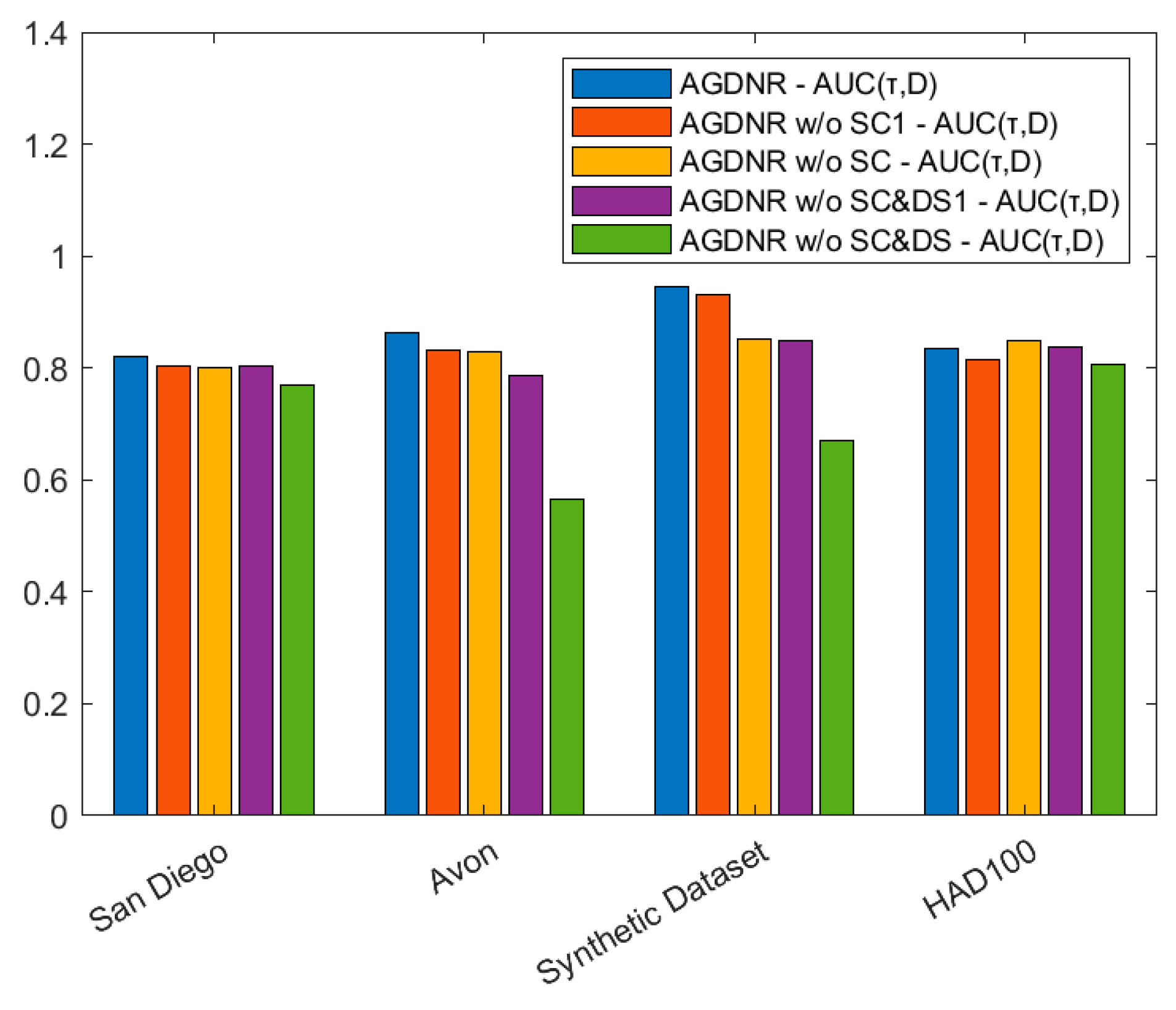
- (1)
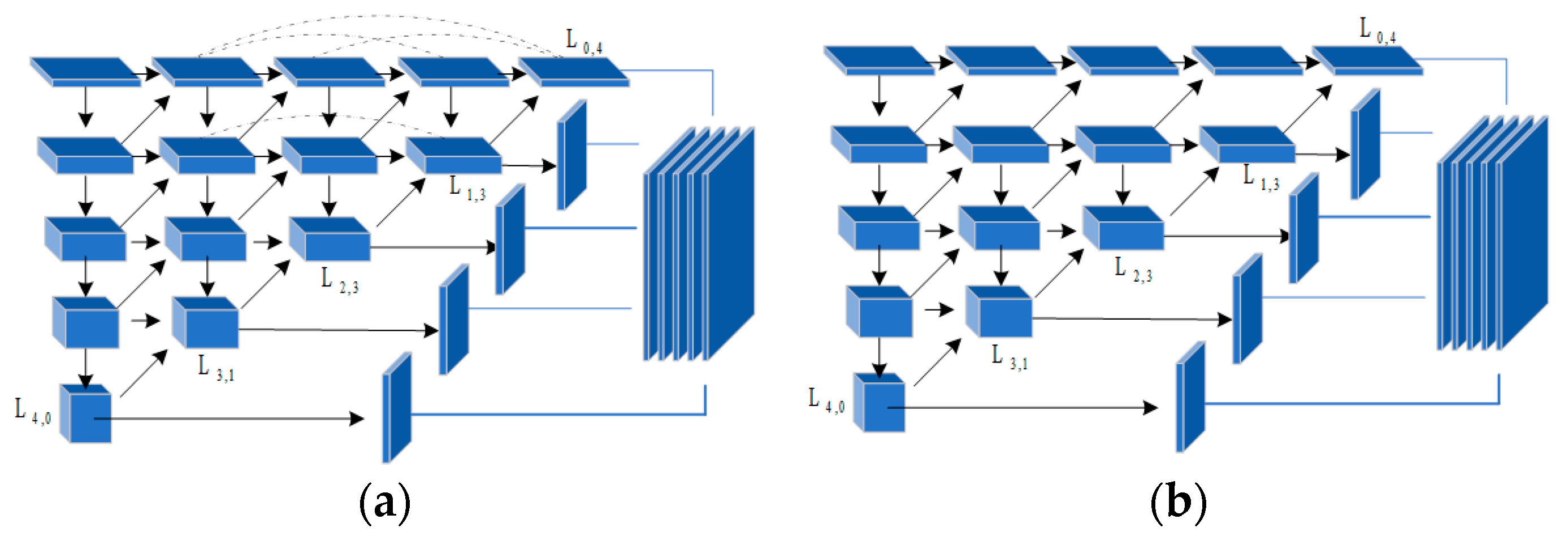
- AGDNR without SC1: As shown in Figure 12a, we removed the skip connection layer between the nodes in the first column and subsequent nodes, preventing the raw information from the preceding layer from being passed to the subsequent network layers.
- (2)
- AGDNR without SC&DS1: As depicted in Figure 12b, we eliminated the down-sampling layer in the first row, hindering the transfer of detailed information from the upper layers to the lower network layers.
3.5.2. Data Ablation
4. Conclusions
Author Contributions
Funding
Data Availability Statement
Conflicts of Interest
References
- Kruse, F.A.; Lefkoff, A.B.; Boardman, J.W.; Heidebrecht, K.B.; Shapiro, A.T.; Barloon, P.J.; Goetz, A.F.H. The Spectral Image Processing System (SIPS)—Interactive Visualization and Analysis of Imaging Spectrometer Data. Remote Sens. Environ. 1993, 44, 145–163. [Google Scholar] [CrossRef]
- Nasrabadi, N.M. Regularized Spectral Matched Filter for Target Recognition in Hyperspectral Imagery. IEEE Signal Process. Lett. 2008, 15, 317–320. [Google Scholar] [CrossRef]
- Farrand, W.H.; Harsanyi, J.C. Mapping the Distribution of Mine Tailings in the Coeur d’Alene River Valley, Idaho, through the Use of a Constrained Energy Minimization Technique. Remote Sens. Environ. 1997, 59, 64–76. [Google Scholar] [CrossRef]
- Chang, C.-I. Orthogonal Subspace Projection (OSP) Revisited: A Comprehensive Study and Analysis. IEEE Trans. Geosci. Remote Sens. 2005, 43, 502–518. [Google Scholar] [CrossRef]
- Zhao, R.; Shi, Z.; Zou, Z.; Zhang, Z. Ensemble-Based Cascaded Constrained Energy Minimization for Hyperspectral Target Detection. Remote Sens. 2019, 11, 1310. [Google Scholar] [CrossRef]
- Chen, S.-Y.; Lin, C.; Tai, C.-H.; Chuang, S.-J. Adaptive Window-Based Constrained Energy Minimization for Detection of Newly Grown Tree Leaves. Remote Sens. 2018, 10, 96. [Google Scholar] [CrossRef]
- Wang, T.; Du, B.; Zhang, L. A Kernel-Based Target-Constrained Interference-Minimized Filter for Hyperspectral Sub-Pixel Target Detection. IEEE J. Sel. Top. Appl. Earth Obs. Remote Sens. 2013, 6, 626–637. [Google Scholar] [CrossRef]
- Chang, C.-I. Hyperspectral Target Detection: Hypothesis Testing, Signal-to-Noise Ratio, and Spectral Angle Theories. IEEE Trans. Geosci. Remote Sens. 2022, 60, 5505223. [Google Scholar] [CrossRef]
- Du, Q.; Ren, H.; Chang, C.-I. A Comparative Study for Orthogonal Subspace Projection and Constrained Energy Minimization. IEEE Trans. Geosci. Remote Sens. 2003, 41, 1525–1529. [Google Scholar] [CrossRef]
- Chang, C.-I.; Ren, H. An Experiment-Based Quantitative and Comparative Analysis of Target Detection and Image Classification Algorithms for Hyperspectral Imagery. IEEE Trans. Geosci. Remote Sens. 2000, 38, 1044–1063. [Google Scholar] [CrossRef]
- Nasrabadi, N.M.; Kwon, H. Kernel Spectral Matched Filter for Hyperspectral Target Detection. In Proceedings of the Proceedings. (ICASSP ’05). IEEE International Conference on Acoustics, Speech, and Signal Processing, Philadelphia, PA, USA, 23–23 March 2005; Volume 4, pp. iv/665–iv/668. [Google Scholar]
- Kwon, H.; Nasrabadi, N.M. Kernel Matched Subspace Detectors for Hyperspectral Target Detection. IEEE Trans. Pattern Anal. Mach. Intell. 2006, 28, 178–194. [Google Scholar] [CrossRef] [PubMed]
- Capobianco, L.; Garzelli, A.; Camps-Valls, G. Target Detection With Semisupervised Kernel Orthogonal Subspace Projection. IEEE Trans. Geosci. Remote Sens. 2009, 47, 3822–3833. [Google Scholar] [CrossRef]
- Ma, K.Y.; Chang, C.-I. Kernel-Based Constrained Energy Minimization for Hyperspectral Mixed Pixel Classification. IEEE Trans. Geosci. Remote Sens. 2022, 60, 5510723. [Google Scholar] [CrossRef]
- Kwon, H.; Nasrabadi, N.M. Hyperspectral Target Detection Using Kernel Spectral Matched Filter. In Proceedings of the 2004 Conference on Computer Vision and Pattern Recognition Workshop, Washington, DC, USA, 27 June 2004–2 July 2004; p. 127. [Google Scholar]
- Dong, Y.; Du, B.; Zhang, L. Target Detection Based on Random Forest Metric Learning. IEEE J. Sel. Top. Appl. Earth Obs. Remote Sens. 2015, 8, 1830–1838. [Google Scholar] [CrossRef]
- Sun, X.; Qu, Y.; Gao, L.; Sun, X.; Qi, H.; Zhang, B.; Shen, T. Target Detection Through Tree-Structured Encoding for Hyperspectral Images. IEEE Trans. Geosci. Remote Sens. 2021, 59, 4233–4249. [Google Scholar] [CrossRef]
- Chen, Y.; Nasrabadi, N.M.; Tran, T.D. Sparse Representation for Target Detection in Hyperspectral Imagery. IEEE J. Sel. Top. Signal Process. 2011, 5, 629–640. [Google Scholar] [CrossRef]
- Li, W.; Du, Q.; Zhang, B. Combined Sparse and Collaborative Representation for Hyperspectral Target Detection. Pattern Recognit. 2015, 48, 3904–3916. [Google Scholar] [CrossRef]
- Zhu, D.; Du, B.; Zhang, L. Binary-Class Collaborative Representation for Target Detection in Hyperspectral Images. IEEE Geosci. Remote Sens. Lett. 2019, 16, 1100–1104. [Google Scholar] [CrossRef]
- Xu, Y.; Wu, Z.; Chanussot, J.; Wei, Z. Joint Reconstruction and Anomaly Detection From Compressive Hyperspectral Images Using Mahalanobis Distance-Regularized Tensor RPCA. IEEE Trans. Geosci. Remote Sens. 2018, 56, 2919–2930. [Google Scholar] [CrossRef]
- Wang, T.; Zhang, H.; Lin, H.; Jia, X. A Sparse Representation Method for a Priori Target Signature Optimization in Hyperspectral Target Detection. IEEE Access 2018, 6, 3408–3424. [Google Scholar] [CrossRef]
- Du, J.; Li, Z.; Sun, H. CNN-Based Target Detection in Hyperspectral Imagery. In Proceedings of the IGARSS 2018—2018 IEEE International Geoscience and Remote Sensing Symposium, Valencia, Spain, 22–27 July 2018; pp. 2761–2764. [Google Scholar]
- Zhang, G.; Zhao, S.; Li, W.; Du, Q.; Ran, Q.; Tao, R. HTD-Net: A Deep Convolutional Neural Network for Target Detection in Hyperspectral Imagery. Remote Sens. 2020, 12, 1489. [Google Scholar] [CrossRef]
- Zhu, D.; Du, B.; Zhang, L. Two-Stream Convolutional Networks for Hyperspectral Target Detection. IEEE Trans. Geosci. Remote Sens. 2021, 59, 6907–6921. [Google Scholar] [CrossRef]
- Yao, C.; Yuan, Y.; Jiang, Z. Self-Supervised Spectral Matching Network for Hyperspectral Target Detection. In Proceedings of the 2021 IEEE International Geoscience and Remote Sensing Symposium IGARSS, Brussels, Belgium, 11–16 July 2021; pp. 2524–2527. [Google Scholar]
- Wang, Y.; Chen, X.; Zhao, E.; Song, M. Self-Supervised Spectral-Level Contrastive Learning for Hyperspectral Target Detection. IEEE Trans. Geosci. Remote Sens. 2023, 61, 5510515. [Google Scholar] [CrossRef]
- Sun, Q.; Liu, Y.; Sheng, C.; Wang, H.; Lu, X. Regions of Interest Extraction for Hyperspectral Small Targets Based on Self-Supervised Learning. IEEE Geosci. Remote Sens. Lett. 2024, 21, 1–5. [Google Scholar] [CrossRef]
- Chen, X.; Zhang, Y.; Dong, Y.; Du, B. Generative Self-Supervised Learning With Spectral-Spatial Masking for Hyperspectral Target Detection. IEEE Trans. Geosci. Remote Sens. 2024, 62, 5522713. [Google Scholar] [CrossRef]
- Shi, Y.; Li, J.; Li, Y.; Du, Q. Sensor-Independent Hyperspectral Target Detection With Semisupervised Domain Adaptive Few-Shot Learning. IEEE Trans. Geosci. Remote Sens. 2021, 59, 6894–6906. [Google Scholar] [CrossRef]
- Li, B.; Xiao, C.; Wang, L.; Wang, Y.; Lin, Z.; Li, M.; An, W.; Guo, Y. Dense Nested Attention Network for Infrared Small Target Detection. IEEE Trans. Image Process. 2023, 32, 1745–1758. [Google Scholar] [CrossRef]
- Marino, K.; Salakhutdinov, R.; Gupta, A. The More You Know: Using Knowledge Graphs for Image Classification. In Proceedings of the 2017 IEEE Conference on Computer Vision and Pattern Recognition (CVPR), Honolulu, HI, USA, 21–26 July 2017; pp. 20–28. [Google Scholar]
- Chen, X.; Li, L.-J.; Fei-Fei, L.; Gupta, A. Iterative Visual Reasoning Beyond Convolutions. In Proceedings of the 2018 IEEE/CVF Conference on Computer Vision and Pattern Recognition, Salt Lake City, UT, USA, 18–23 June 2018; pp. 7239–7248. [Google Scholar]
- Xu, H.; Jiang, C.; Liang, X.; Lin, L.; Li, Z. Reasoning-RCNN: Unifying Adaptive Global Reasoning Into Large-Scale Object Detection. In Proceedings of the 2019 IEEE/CVF Conference on Computer Vision and Pattern Recognition (CVPR), Long Beach, CA, USA, 15–20 June 2019; pp. 6412–6421. [Google Scholar]
- Qian, Y.; Pu, X.; Jia, H.; Wang, H.; Xu, F. ARNet: Prior Knowledge Reasoning Network for Aircraft Detection in Remote-Sensing Images. IEEE Trans. Geosci. Remote Sens. 2024, 62, 1–14. [Google Scholar] [CrossRef]
- Li, S.; Dian, R.; Liu, H. Learning the External and Internal Priors for Multispectral and Hyperspectral Image Fusion. Sci. China Inf. Sci. 2023, 66, 140303. [Google Scholar] [CrossRef]
- Van de Griend, A.A.; Owe, M. On the Relationship between Thermal Emissivity and the Normalized Difference Vegetation Index for Natural Surfaces. Int. J. Remote Sens. 1993, 14, 1119–1131. [Google Scholar] [CrossRef]
- Xie, Q.; Huang, W.; Liang, D.; Chen, P.; Wu, C.; Yang, G.; Zhang, J.; Huang, L.; Zhang, D. Leaf Area Index Estimation Using Vegetation Indices Derived From Airborne Hyperspectral Images in Winter Wheat. IEEE J. Sel. Top. Appl. Earth Obs. Remote Sens. 2014, 7, 3586–3594. [Google Scholar] [CrossRef]
- Huete, A.R. A Soil-Adjusted Vegetation Index (SAVI). Remote Sens. Environ. 1988, 25, 295–309. [Google Scholar] [CrossRef]
- Jing, L.I.; Hanqiu, X.U.; Xia, L.I.; Yanbin, G.U.O. Vegetation Information Extraction of Pinus Massoniana Forest in Soil Erosion Areas Using Soil-Adjusted Vegetation Index. J. Geo-Inf. Sci. 2015, 17, 1128–1134. [Google Scholar] [CrossRef]
- MAJOR, D.J.; BARET, F.; GUYOT, G. A Ratio Vegetation Index Adjusted for Soil Brightness. Int. J. Remote Sens. 1990, 11, 727–740. [Google Scholar] [CrossRef]
- Wang, C.; Qi, S.; Niu, Z.; Wang, J. Evaluating Soil Moisture Status in China Using the Temperature–Vegetation Dryness Index (TVDI). Can. J. Remote Sens. 2004, 30, 671–679. [Google Scholar] [CrossRef]
- JPL|AVIRIS Data Portal. Available online: https://aviris.jpl.nasa.gov/dataportal/ (accessed on 1 December 2024).
- (PDF) The SHARE 2012 Data Campaign. Available online: https://www.researchgate.net/publication/260782828_The_SHARE_2012_data_campaign (accessed on 1 December 2024).
- Liu, K.; Zhou, Z.; Li, S.Y.; Liu, Y.F.; Wan, X.; Liu, Z.W.; Tan, H.; Zhang, W.F. Scene classification dataset using the Tiangong-1 hyperspectral remote sensing imagery and its applications. Natl. Remote Sens. Bull. 2020, 24, 1077–1087. [Google Scholar] [CrossRef]
- Sun, X.T. Sxt1996/Airport-Beach-Urban-ABU. Available online: https://github.com/sxt1996/Airport-Beach-Urban-ABU (accessed on 1 December 2024).
- Li, Z.; Wang, Y.; Xiao, C.; Ling, Q.; Lin, Z.; An, W. You Only Train Once: Learning a General Anomaly Enhancement Network with Random Masks for Hyperspectral Anomaly Detection. IEEE Trans. Geosci. Remote Sens. 2023, 61, 5506718. [Google Scholar] [CrossRef]
- Zhu, D.; Du, B.; Zhang, L. Target Dictionary Construction-Based Sparse Representation Hyperspectral Target Detection Methods. IEEE J. Sel. Top. Appl. Earth Obs. Remote Sens. 2019, 12, 1254–1264. [Google Scholar] [CrossRef]
- Zhao, C.; Wang, M.; Feng, S.; Su, N. Hyperspectral Target Detection Method Based on Nonlocal Self-Similarity and Rank-1 Tensor. IEEE Trans. Geosci. Remote Sens. 2022, 60, 5500815. [Google Scholar] [CrossRef]
- Chang, C.-I. An Effective Evaluation Tool for Hyperspectral Target Detection: 3D Receiver Operating Characteristic Curve Analysis. IEEE Trans. Geosci. Remote Sens. 2021, 59, 5131–5153. [Google Scholar] [CrossRef]
- Kraut, S.; Scharf, L.L. The CFAR Adaptive Subspace Detector Is a Scale-Invariant GLRT. IEEE Trans. Signal Process. 1999, 47, 2538–2541. [Google Scholar] [CrossRef]
- Wang, Y.; Chen, X.; Wang, F.; Song, M.; Yu, C. Meta-Learning Based Hyperspectral Target Detection Using Siamese Network. IEEE Trans. Geosci. Remote Sens. 2022, 60, 5527913. [Google Scholar] [CrossRef]
- Jiao, J.; Gong, Z.; Zhong, P. Triplet Spectralwise Transformer Network for Hyperspectral Target Detection. IEEE Trans. Geosci. Remote Sens. 2023, 61, 5519817. [Google Scholar] [CrossRef]
- Yang, Q.; Wang, X.; Chen, L.; Zhou, Y.; Qiao, S. CS-TTD: Triplet Transformer for Compressive Hyperspectral Target Detection. IEEE Trans. Geosci. Remote Sens. 2024, 62, 5533115. [Google Scholar] [CrossRef]


| NDVI Interval | Land Surface Type |
|---|---|
| water, clouds, or oceans | |
| urban | |
| soil | |
| soil/vegetation mixed area | |
| vegetation |
| Dataset | Train or test | Category 1 | Category 2 | Category 3 | Category 4 | All Categories |
|---|---|---|---|---|---|---|
| San Diego dataset | train | 5 | 2 | 11 | -- | 18 |
| test | 15 | 6 | 38 | -- | 59 | |
| Avon dataset | train | 4 | 4 | 0.5 | 0.3 | 8.8 |
| test | 12 | 12 | 2 | 1 | 27 | |
| Synthetic dataset | train | 5 | 5 | 5 | -- | 15 |
| test | 15 | 15 | 15 | -- | 45 | |
| HAD100 dataset | train | 6 | 6 | 4 | 4 | 20 |
| test | 26 | 25 | 13 | 13 | 77 |
| Dataset | AUC | ACE | E-CEM | HTD-IRN | TSSTD | CS-TTD | AGDNR |
|---|---|---|---|---|---|---|---|
| San Diego dataset | 0.673917 | 0.904242 | 0.769122 | 0.832509 | 0.910121 | 0.999537 | |
| 0.986446 | 0.160722 | 0.024773 | 0.025760 | 0.698200 | 0.805841 | ||
| 0.965915 | 0.064171 | 0.004925 | 0.001483 | 0.205343 | 0.006516 | ||
| Avon dataset | 0.753610 | 0.899847 | 0.898329 | 0.954091 | 0.988532 | 0.999844 | |
| 0.904321 | 0.498903 | 0.026905 | 0.061970 | 0.809364 | 0.831935 | ||
| 0.872586 | 0.300727 | 0.015234 | 0.003224 | 0.041702 | 0.000284 | ||
| Synthetic dataset | 0.423741 | 0.630519 | 0.491987 | 0.999370 | 1.000000 | 1.000000 | |
| 0.466774 | 0.476457 | 0.514915 | 0.375661 | 0.998860 | 0.858989 | ||
| 0.439160 | 0.402847 | 0.495558 | 0.000497 | 0.003939 | 0.000005 | ||
| HAD100 dataset | 0.793811 | 0.935234 | 0.698967 | 0.811994 | 0.626478 | 0.999534 | |
| 0.895538 | 0.504348 | 0.549460 | 0.024640 | 0.278232 | 0.808148 | ||
| 0.559483 | 0.015566 | 0.332796 | 0.002070 | 0.181698 | 0.001311 |
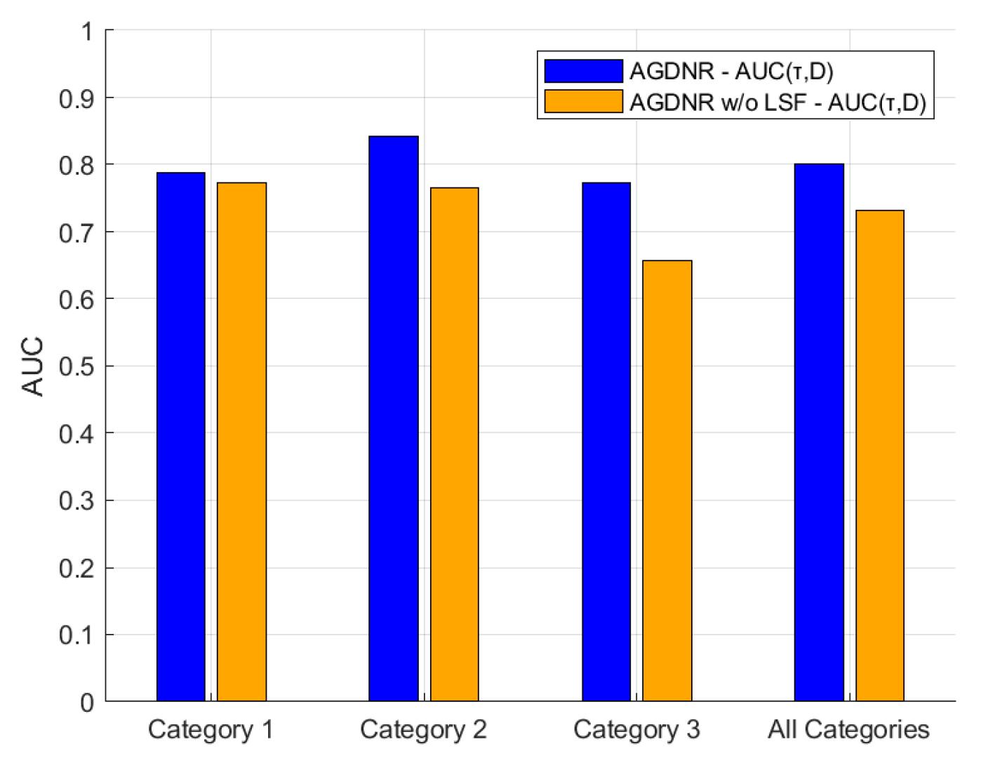
| Dataset | AUC | Category 1 | Category 2 | Category 3 | Category 4 | All Categories |
|---|---|---|---|---|---|---|
| San Diego | 0.999768 | 0.999904 | 0.999846 | -- | 0.999829 | |
| 0.787623 | 0.842028 | 0.772183 | -- | 0.800620 | ||
| 0.000495 | 0.000387 | 0.000610 | -- | 0.000497 | ||
| Masic Avon | 0.999990 | 0.999836 | 0.999996 | 0.999984 | 0.999947 | |
| 0.861449 | 0.773185 | 0.733864 | 0.861592 | 0.811629 | ||
| 0.000136 | 0.000110 | 0.000029 | 0.000087 | 0.000089 | ||
| Synthetic dataset | 1.000000 | 1.000000 | 1.000000 | -- | 1.000000 | |
| 0.799914 | 0.895986 | 0.716441 | -- | 0.775847 | ||
| 0.000005 | 0.000005 | 0.000022 | -- | 0.000007 | ||
| HAD100 | 0.999995 | 0.999863 | 0.999672 | 0.999992 | 0.999868 | |
| 0.862036 | 0.807737 | 0.712738 | 0.658273 | 0.796993 | ||
| 0.000185 | 0.000617 | 0.000327 | 0.000339 | 0.000356 |
| Model | Dataset | |||
|---|---|---|---|---|
| San Diego Dataset | Avon Dataset | Synthetic Dataset | HAD100 Dataset | |
| AGDNR | 0.806 | 0.899 | 1.000 | 0.820 |
| AGDNR w/o SC1 | 0.778 | 0.869 | 1.000 | 0.844 |
| AGDNR w/o SC | 0.776 | 0.883 | 0.944 | 0.810 |
| AGDNR w/o SC&DS1 | 0.760 | 0.883 | 0.930 | 0.800 |
| AGDNR w/o SC&DS | 0.758 | 0.630 | 0.793 | 0.796 |
Disclaimer/Publisher’s Note: The statements, opinions and data contained in all publications are solely those of the individual author(s) and contributor(s) and not of MDPI and/or the editor(s). MDPI and/or the editor(s) disclaim responsibility for any injury to people or property resulting from any ideas, methods, instructions or products referred to in the content. |
© 2025 by the authors. Licensee MDPI, Basel, Switzerland. This article is an open access article distributed under the terms and conditions of the Creative Commons Attribution (CC BY) license (https://creativecommons.org/licenses/by/4.0/).
Share and Cite
Zhan, S.; Yang, Y.; Zhong, M.; Lu, G.; Zhou, X. Adaptive Global Dense Nested Reasoning Network into Small Target Detection in Large-Scale Hyperspectral Remote Sensing Image. Remote Sens. 2025, 17, 948. https://doi.org/10.3390/rs17060948
Zhan S, Yang Y, Zhong M, Lu G, Zhou X. Adaptive Global Dense Nested Reasoning Network into Small Target Detection in Large-Scale Hyperspectral Remote Sensing Image. Remote Sensing. 2025; 17(6):948. https://doi.org/10.3390/rs17060948
Chicago/Turabian StyleZhan, Siyu, Yuxuan Yang, Muge Zhong, Guoming Lu, and Xinyu Zhou. 2025. "Adaptive Global Dense Nested Reasoning Network into Small Target Detection in Large-Scale Hyperspectral Remote Sensing Image" Remote Sensing 17, no. 6: 948. https://doi.org/10.3390/rs17060948
APA StyleZhan, S., Yang, Y., Zhong, M., Lu, G., & Zhou, X. (2025). Adaptive Global Dense Nested Reasoning Network into Small Target Detection in Large-Scale Hyperspectral Remote Sensing Image. Remote Sensing, 17(6), 948. https://doi.org/10.3390/rs17060948