INS/LiDAR Relative Navigation Design Based on Point Cloud Covariance Characteristics for Spacecraft Proximity Operation

Abstract

This paper proposes a pose estimation algorithm using INS and LiDAR for precise cooperative relative navigation between target and chaser spacecraft in a close docking mission scenario. Previous cooperative algorithms have proposed estimating position and pose transformations using typical matching methods or to pre-extract and utilize features from point cloud data. However, in the case of general proximity rendezvous docking, a straight-line approach scenario with very few changes in attitude is usually assumed, and, in this case, pose estimation using simple matching techniques or feature point extraction leads to inaccurate results. To solve this problem, this paper performed a principal component analysis (PCA) based on ICP to align the initial transformation matrix. To keep the distribution of point cloud data constant, the point cloud at the time of docking was applied to ICP to minimize the change in the distribution of point clouds over time. Finally, we designed an EKF filter that estimates the relative position, velocity, and attitude using the INS model and combines it with the relative pose estimated from the point cloud; the proposed method showed the results of estimating the relative pose more effectively than the previous method. The simulation and experiment showed more accurate estimation results than the ICP method in position and attitude, respectively. In particular, in the case of position, both the simulation and experiment showed 0.46 m and 0.32 m better estimation results in the z-axis. Also, attitude estimation showed 0.11° and 2.66° better results in roll and 0.01° and 0.34° better results in pitch. This shows that the proposed algorithm provided better pose estimation results in the docking scenario in a straight line.

1. Introduction

With the increasing interest in performing various missions in space, research on precise mission performance using sensors such as camera and LiDAR has been actively conducted. Unlike the ground environment, the space environment often utilizes prior data about the target of the mission, and it is important to estimate the position and attitude accurately by combining them with the data of the chaser. Therefore, research using various sensors in the space environment [1,2,3,4] is actively being conducted, and recently, research using point cloud data obtained by TOF cameras or LiDAR sensors [5,6] has been developed. Mission performance in the space environment can be categorized into cooperative and non-collaborative mission performance [7], depending on whether the information of the target is utilized in advance.

In the case of non-cooperative missions, there is no information about the target, so pose estimation is performed using data obtained from the sensors of the chaser. Therefore, it is important to efficiently use the measurement data of the target, and the main objective is to accurately estimate the position and pose through the three-dimensional data of the point cloud.

To achieve this, many existing studies have proposed methods for efficiently extracting feature points of point clouds [8,9,10,11] or using geometric characteristics [12]. On the other hand, in cooperative missions, prior information is often available, and accurate navigation information of the target can be delivered when necessary. Therefore, in this case, the effective use of prior point cloud data is a key point, and more accurate pose estimation can be achieved by properly combining measurements and prior information.

In pose estimation using point cloud data, the initial pose transformation matrix is a very important factor. Previous studies [13,14,15] have used PCA to obtain the initial pose transformation or have optimized point cloud matching by adding specific weights. However, these methods have problems in scenarios such as rendezvous/docking, where the distribution of point clouds continually changes, leading to inaccurate estimations.

In the cases of papers that use point cloud data in the space environment, the position and attitude results obtained through ICP are used as measurements, and to improve the accuracy of measurement, various algorithms are applied to the ICP method. The ICP algorithm is sensitive to the initial transformation matrix, and, as a result, techniques to calculate more accurate initial attitude measurements have been developed. Among these, the PCA method, which estimates the initial attitude based on the distribution of point cloud data, is also widely used. In this paper, we propose a cooperative matching-based principal component analysis that uses PCA to calculate the covariance of point cloud data and computes a more accurate initial attitude transformation matrix through ICP [16] with the previously obtained point cloud data. Unlike previous papers, in order to utilize the advantage of PCA, which shows better estimation results with small changes in point cloud data, we first use ICP to maintain a consistent distribution of point cloud data over time and then apply the PCA method to estimate the initial transformation matrix. This method has the advantage of keeping the distribution of point clouds constant by matching, enabling accurate estimation of the initial attitude transformation matrix even in proximity scenarios with little attitude change.

After that, the rotation matrix between consecutive frames was calculated through the CMT algorithm [17], and a continuous high-precision pose estimation algorithm was designed through the error-state EKF based on the INS model. Unlike previous studies that estimate position and velocity using orbital equations and estimate attitude using angular velocity, this paper used the INS propagation model based on IMU data. And we proposed an INS/LiDAR combined filter that uses position and attitude calculated through the point cloud algorithm as a measurement. The performance of the algorithm designed through a simulation and experiment was compared and analyzed with the existing methods.

This paper is organized as follows. Section 2 describes the main point cloud data methods, principal component analysis (PCA), and CMT algorithm. Section 3 describes the combined algorithm of E2PCA and CMT and explains the INS model and error-state EKF structure. In Section 4 and Section 5, we analyze the performance of the algorithm based on simulation and experimental results, respectively. Section 6 is the discussion, which includes an analysis of the algorithm explained in the paper, and finally Section 7 contains the conclusion of the paper.

2. Background Methods

2.1. PCA Method

The point cloud data obtained by the LiDAR sensor are 3D data and have coordinated information about three axes. For accurate pose estimation, it is important to align the rotation axes of three-dimensional data, and the normal vector of point cloud data is useful for initial rotation axis alignment. The PCA (point cloud component analysis) technique is one of the representative techniques of dimension reduction and is used to determine the distribution of data by calculating eigenvectors and eigenvalues using the covariance of data. The formula for the covariance matrix of the entire point cloud data of the target is as follows.

$$C_i={\displaystyle \frac{1}{n}}{\sum }_{k=1}^n\left(P_{i,k}-\overline{P_i}\right){\left(P_{i,k}-\overline{P_i}\right)}^T,$$

(1)

$$\overline{P_i}={\displaystyle \frac{1}{n}}{\sum }_{k=1}^n{P}_{i,k},$$

(2)

${\mathit{P}}_{\mathit{i},\mathit{k}}$ means the $k$-$th$ point of the point cloud data obtained at time $\mathit{i}$, and ${\mathit{P}}_{\mathit{i}}$ in Equation (2) means the center of the point cloud data. The relationship between the eigenvalues and eigenvectors of the covariance matrix calculated in this way is as follows.

$$C_i·{\overrightarrow{v}}_{\mathrm{1,2},3}={\lambda }_{\mathrm{1,2},3}·{\overrightarrow{v}}_{\mathrm{1,2},3 },$$

(3)

${\overrightarrow{\mathit{v}}}_{\mathbf{1},\mathbf{2},\mathbf{3}}$ mean each of the three eigenvectors of the covariance matrix, and ${\mathit{\lambda }}_{\mathbf{1},\mathbf{2},\mathbf{3}}$ mean each eigenvalue. The eigenvector corresponding to ${\mathit{\lambda }}_{\mathbf{1}}$ with the largest eigenvalue is ${\overrightarrow{\mathit{v}}}_{\mathbf{1}}$, and this eigenvector represents the direction in which the data are the most distributed. Figure 1 shows an example of the distribution and eigenvector orientation of point cloud data obtained using the PCA method.

The red vector with the largest variance is the principal component vector of the point cloud and represents the direction in which the points are the most distributed. The green vector is the next vector with the largest variance and the second vector with the best distribution of points. The first and second vectors lie on the same plane, and the last blue vector with the smallest variance is perpendicular to this plane.

2.2. CMT Method

Section 2.2 describes the CMT algorithm. The CMT algorithm [17] is a matching algorithm that uses the relationship between the covariances of consecutive point cloud data. The covariance matrix of a point cloud at time $\mathit{i}$ is given below.

$$C_i={\displaystyle \frac{1}{n}}{\sum }_{k=1}^n{\xi }_{i,k}\left(P_{i,k}-\overline{P_i}\right){\left(P_{i,k}-\overline{P_i}\right)}^T,$$

(4)

$${\xi }_{i,k}={\displaystyle \frac{1}{‖P_{i,k}-\overline{P_i}‖}},$$

(5)

The covariance matrix for the point cloud data at time $\mathit{i}$ is shown in Equation (4), and its center point and coefficient correspond to (2) and (5), respectively. Assuming that there are point cloud data at time $\mathit{i}$ and $\mathit{j}$, which are consecutive frames, the relationship between the two-point cloud data is expressed as shown in Equation (6) below.

$$P_j=R·P_i+t,$$

(6)

$$C_j={\displaystyle \frac{1}{n}}{\sum }_{k=1}^n{\xi }_{j,k}\left(P_{j,k}-\overline{P_j}\right){\left(P_{j,k}-\overline{P_j}\right)}^T,$$

(7)

If the covariance matrix of the point cloud data at time $\mathit{j}$ is similarly expanded, it is the same as Equation (7), and, using the previous equations, it can be expressed as a relation between the covariance and rotation between the time $\mathit{i}$ and time $\mathit{j}$ point clouds, as shown in Equation (8).

$$C_j={\displaystyle \frac{1}{n}}{\sum }_{k=1}^n{\xi }_{j,k}\left(P_{j,k}-\overline{P_j}\right){\left(P_{j,k}-\overline{P_j}\right)}^T={\displaystyle \frac{1}{n}}{\sum }_{k=1}^n{\xi }_{i,k}\left\{R\left(P_{i,k}-\overline{P_i}\right)\right\}\{R{\left(P_{i,k}-\overline{P_i}\right)\}}^T=R·C_i·R^T,$$

(8)

If the eigenvalues and eigenvectors of the covariance ${\mathit{C}}_{\mathit{i}}$ obtained in the same way as in Section 2.1 are $\mathit{\lambda }$ and $\overrightarrow{\mathit{v}}$, respectively, Equation (8) can be expressed as follows.

$$C_j=R{C}_i{R}^T \to \lambda ·\overrightarrow{n}=R^T{·C}_j·R·\overrightarrow{n},$$

(9)

To optimize Equation (9), we can transform it into an objective function form and summarize it using Lie Algebra as follows.

$$\begin{array}{r}f\left(R\right)={‖R^T{·C}_j·R·\overrightarrow{n}-\lambda ·\overrightarrow{n}‖}_2^2\to f\left(\phi \right)={‖\mathrm{e}\mathrm{x}\mathrm{p}\left({-\phi }^{\wedge }\right){·C}_j·\mathrm{e}\mathrm{x}\mathrm{p}\left({\phi }^{\wedge }\right)·\overrightarrow{n}-\lambda ·\overrightarrow{n}‖}_2^2\\ ={\overrightarrow{n}}^T\exp \left({-\phi }^{\wedge }\right){C_j}^2\exp \left({\phi }^{\wedge }\right)\overrightarrow{n}-2\lambda {\overrightarrow{n}}^T\exp \left({-\phi }^{\wedge }\right)C_j\exp \left({\phi }^{\wedge }\right)\overrightarrow{n}+{\lambda }^2{\overrightarrow{n}}^T\overrightarrow{n}\end{array},$$

(10)

$$\exp \left({\phi }^{\wedge }\right)\approx 1+{\phi }^{\wedge },$$

(11)

To calculate the Jacobian of Equation (10), we apply the Perturbation Model and summarize it using the Taylor series to obtain Equation (12).

$$\begin{array}{r}J={\displaystyle \frac{\partial f\left(∆R·R\right)}{\partial \phi }}=\underset{\phi \to 0}{\lim }{\displaystyle \frac{{\overrightarrow{n}}^T\exp \left({-\phi }^{\wedge }\right){C_j}^2\exp \left({\phi }^{\wedge }\right)\overrightarrow{n}-2\lambda {\overrightarrow{n}}^T\exp \left({-\phi }^{\wedge }\right)C_j\exp \left({\phi }^{\wedge }\right)\overrightarrow{n}+{\lambda }^2{\overrightarrow{n}}^T\overrightarrow{n}-f\left(R\right)}{\phi }}\\ ={\overrightarrow{n}}^T\exp \left({-\phi }^{\wedge }\right){C_j}^2\exp \left({\phi }^{\wedge }\right)\overrightarrow{n}-2\lambda {\overrightarrow{n}}^T\exp \left({-\phi }^{\wedge }\right)C_j\exp \left({\phi }^{\wedge }\right)\overrightarrow{n}+{\lambda }^2{\overrightarrow{n}}^T\overrightarrow{n},\end{array}$$

(12)

Finally, by optimizing the Jacobian using the nonlinear optimization method LM (Levenberg–Marquardt) Algorithm [18], the rotational transformation matrix ${\mathit{R}}^{\ast }$ and the translation distance ${\mathit{t}}^{\ast }$ can be calculated.

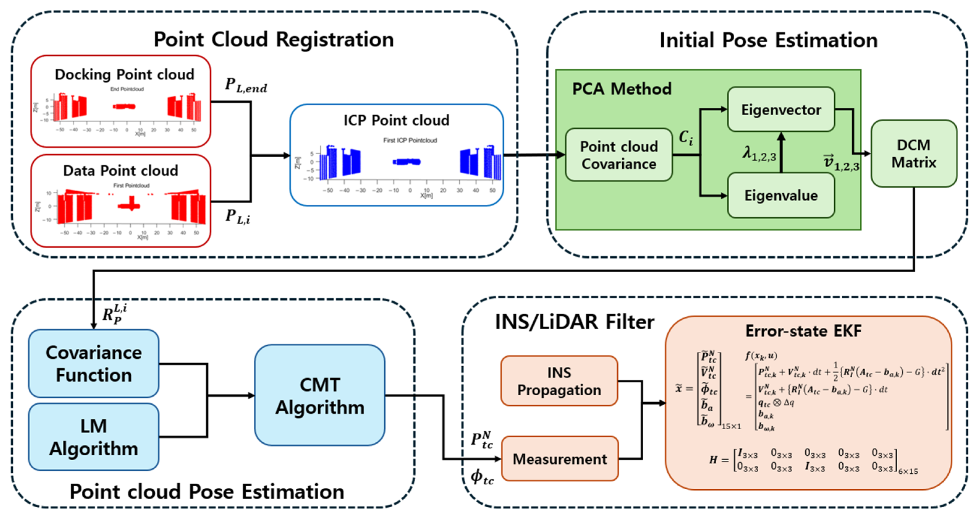
3. Point Cloud Pose Estimation

Both PCA and CMT, described in Section 2, are methods that use a point cloud covariance matrix. The original CMT algorithm [17] performed pose estimation for non-cooperative targets without using point cloud features. In this paper, we propose the E2PCA-CMT algorithm, which combines the PCA method and the CMT algorithm to improve the accuracy of pose estimation in cooperative situations where the point cloud data at a specific point cloud in time are known.

Using the PCA method explained in Section 2.1, the covariance matrix of the point cloud data at time $\mathit{i}$ can be obtained. The covariance matrix, eigenvalues, and eigenvectors of the point cloud data can be obtained through Equations (1)–(3), and the three eigenvectors can be used as the initial pose transformation matrix of the point cloud, as shown in Figure 1. In a rendezvous/docking scenario, the eigenvector obtained using the PCA method, knowing the point cloud data at the docking zone, which is the last point of contact, can be expressed as follows.

$${R_P^{L,end}=[{\overrightarrow{v}}_1,{\overrightarrow{v}}_2,{\overrightarrow{v}}_3]}^T,$$

(13)

Since the point cloud data are measured relative to the LiDAR sensor frame, the rotation matrix made from the three eigenvectors obtained through the PCA method becomes the attitude of the PCA three axes viewed from the LiDAR frame. However, if there is a change in the point cloud data, the covariance and variance will change, and as a result, the eigenvectors will also change. Especially for large and complex targets such as the ISS, the change in point clouds can be significant even in a straight approach scenario with little attitude change.

To minimize the change in point clouds, this paper maintained the same shape of point cloud distribution by matching the point cloud data at the time of docking with the point clouds at the current time using the ICP method, as shown in Figure 2. Figure 2a,b show the point cloud data according to distance before using the ICP method, where Figure 2a shows the point cloud of the ISS model before the approach and Figure 2b shows the point cloud of the ISS model at the time of docking. As seen in Figure 2a,b, the point clouds of the ISS model obtained at a distance of 30 m and less than 5 m are significantly different in overall shape and distribution. In order to minimize the change in point cloud distribution and maintain the same shape of point clouds, we employed the ICP registration based on a cooperative situation that uses point cloud data at the last time. To maintain a consistent shape, the LiDAR point cloud obtained in each time step was set as the reference point cloud while the last time point was used as the point cloud data to be registered. Due to the characteristics of ICP, the distribution of the point cloud data obtained as a result of ICP alignment maintains the same shape as the distribution of the point cloud data to be aligned, not the reference point cloud, so the result is always the same distribution and shape as the point cloud data at the last point in time. Figure 2c,d show the point cloud data after ICP alignment, and, unlike Figure 2a,b, it is observed that they all maintain the same point cloud distribution regardless of distance.

By applying the PCA method to the point cloud obtained through ICP matching, the attitude transformation matrix of the point cloud is calculated, and the initial attitude transformation matrix of the point cloud data can be obtained by converting it to the frame of the LiDAR sensor. The equations for the process of matching point clouds through the ICP method and converting them into frames of the LiDAR sensor are shown in Equations (14) and (15).

$$P_i=R_{L,end}^{L,i}·P_{L,end}+t_{L,end\to L,i},$$

(14)

$${R_P^{L,i}=R_{PCA\to LiDAR}·R}_{L,end}^{L,i}·R_P^{L,end},$$

(15)

Equation (14) corresponds to the relationship between the point cloud data at the docking time and the point cloud data at the current time $\mathit{i}$ through ICP matching, and Equation (15) calculates the rotation matrix obtained through Equation (14) and the PCA-based rotation matrix after frame transformation. In this paper, the method of calculating the rotation matrix of PCA using ICP is named E2PCA (Endpoint To PCA).

In the same way, the rotation matrix at time $\mathit{i}+\mathbf{1}$ can be obtained, and the transformation matrix between two consecutive times can be derived as follows.

$$R_{L,i}^{L,i+1}=R_P^{L,i+1}·{{(R}_P^{L,i})}^T,$$

(16)

The ${\mathit{R}}_{\mathit{L},\mathit{i}}^{\mathit{L},\mathit{i}+\mathbf{1}}$ obtained from Equation (16) represents the DCM matrix between consecutive frames, and it is applied in Equation (12) from Section 2.2 as the initial rotation matrix for the nonlinear algorithm. Through this, we reduced the probability of local optima and improved the accuracy of pose estimation by using appropriate initial values in situations with little pose variation. In this paper, this algorithm, which combines the previously mentioned E2PCA and CMT, is named the E2PCA-CMT method.

The final relationship of the position and attitude between two consecutive frames obtained through Equations (13) and (16) can be summarized as follows.

$$t_{i\to i+1}=\overline{P_j}-R_{L,i}^{L,i+1}·\overline{P_i},$$

(17)

In order to utilize the position and attitude obtained through Equation (17), this paper combines it with the INS model to design the INS/LiDAR Error-state EKF. The relative position, velocity, and attitude of the target and chaser are updated using the INS model, and measurement updates are performed using the measurements obtained through the E2PCA-CMT method to construct the final relative pose estimation algorithm. The algorithm’s structure is shown in Figure 3.

4. Simulation Study

4.1. Simulation Environment

Section 4.1 describes the configuration and implementation of the simulation environment for algorithm verification. The simulation was performed using a Gazebo simulation, which can generate LiDAR sensor data, and the scenario was configured in the ROS 20.04 environment. To configure the automatic/rendezvous docking scenario, the target was set as ISS, the chaser was set as a LiDAR sensor, and the distance between the target and the chaser was about 30 m.

Table 1. LiDAR sensor specification in Gazebo simulation.

LiDAR Sensor	OS0-64
Maximum range	0.5 m
Minimum range	300 m
Vertical Resolution	64
Horizontal Resolution	1024
Field of View	Horizontal: 360° Vertical: −11.25°~11.25°

summarizes the specifications of the LiDAR sensors used in the simulation.

The sensor simulated Ouster LiDAR, the point cloud data and IMU data were obtained using the ROS topic, and the position and pose data provided by Gazebo simulation were used as reference data. IMU and point cloud data topics were received at 10,010 hz, respectively, and the algorithm results were obtained by using MATLAB R2023b to implement pose estimation method in Section 3. Figure 4 shows the overall configuration of the algorithm using the simulation.

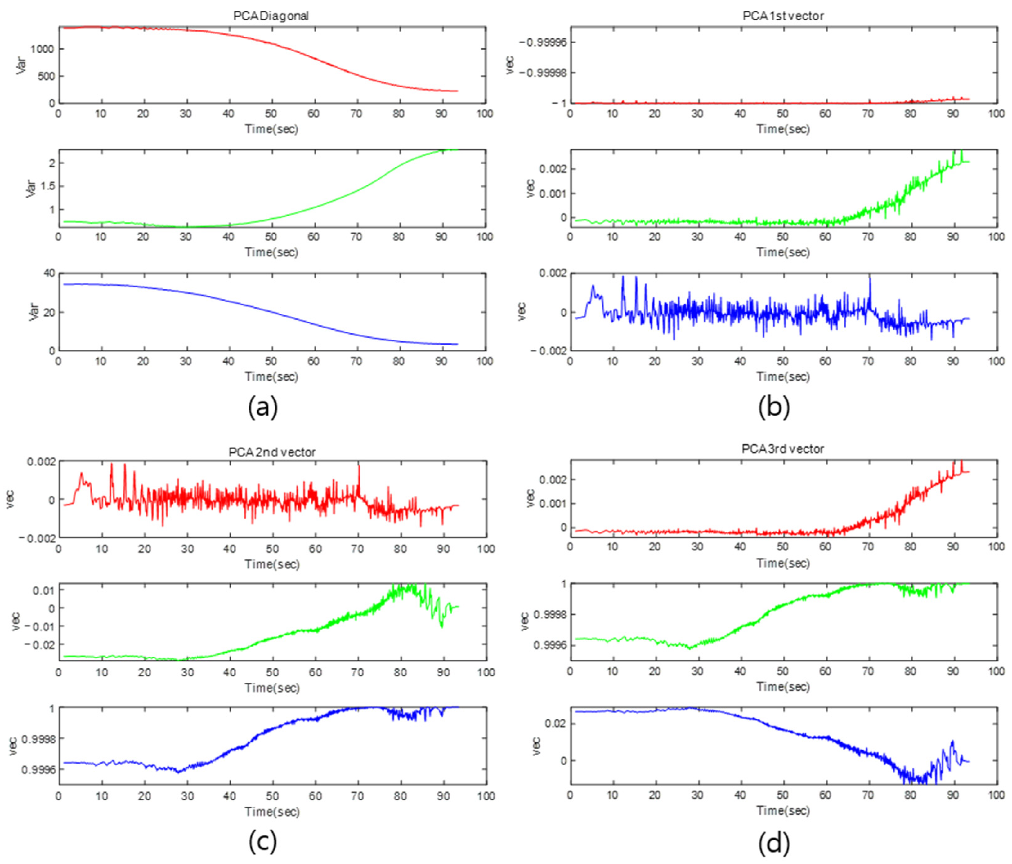
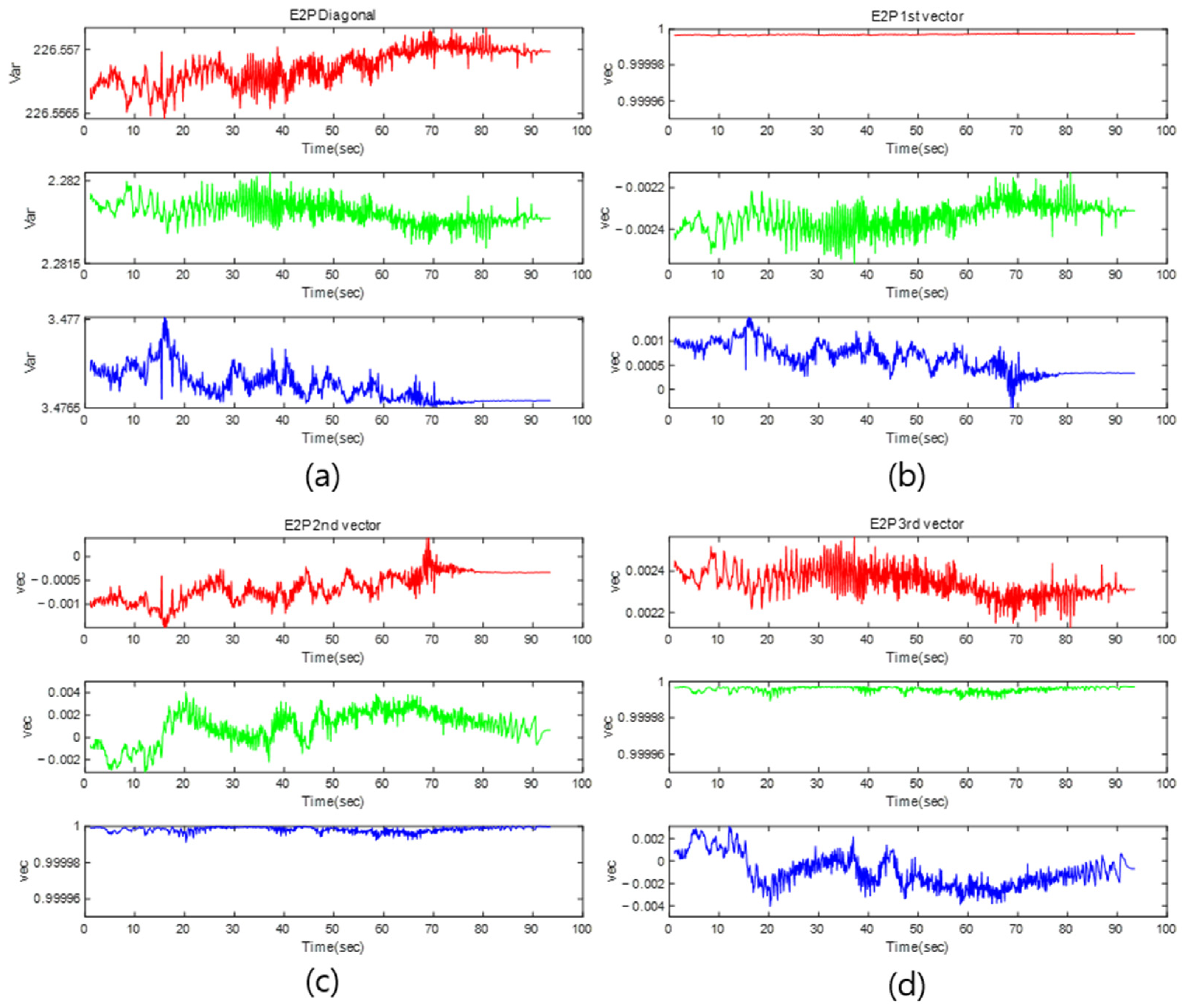
4.2. Simulation Result

First, the covariance matrix of the point cloud data was analyzed for the scenario of approaching the ISS model in a slow, straight-line drive from 30 m. To compare the performance of the principal component analysis (PCA) with and without ICP matching in Section 3, the variance in the covariance matrix and the change in the eigenvectors were compared.

Figure 5 shows the variance and eigenvector changes calculated from the covariance matrix of point cloud data obtained from the LiDAR sensor attached to the chaser. As shown in Figure 5a, the variance in the point cloud changes as the distance to the target decreases, and the direction of the three eigenvectors obtained through PCA changes as well. Figure 5b–d show the change in direction with respect to the three axes of each eigenvector.

In order to maintain the distribution of point clouds and reduce the changes in variance and eigenvectors derived from the covariance matrix, the results of E2PCA using PCA by matching point cloud at docking time through the ICP method are as follows.

Unlike Figure 5, after applying E2PCA, we can see that the variance on each axis remains almost constant, as shown in Figure 6a. Since the distribution of the point cloud data was stabilized using ICP, the variance, which is the diagonal part of the covariance matrix, remains almost unchanged, and the three-axis eigenvectors calculated from this also maintain a constant value even when the distance changes.

The rotation matrix between two consecutive frames can be obtained by using Equation (16) described in Section 3. Pose estimation was performed using the calculated rotation matrix as the initial value of the CMT algorithm, the error-state EKF filter was implemented in combination with the INS model, and the performance was analyzed as shown in Figure 3. To compare the results, the position and attitude results estimated using each algorithm were used as a measurement of filter, and the navigation performance was analyzed using Loosely Coupled EKF after applying the same INS model.

Figure 7a,b show the error results of position and attitude by the algorithm with Error-state EKF. The performance of the E2PCA-CMT algorithm proposed in this paper shows that it provides the most accurate overall estimation of position and attitude. In the case of general ICP, the error is not large in the attitude because it uses point cloud data at the time of docking, but the estimation error is large in the case of poor matching due to the difference in the distribution of the point cloud data, such as the initial part of the position estimation result. It can be seen that the PCA-CMT algorithm without ICP has a relatively large pose error compared to E2PCA-CMT because the initial rotation matrix is not calculated correctly, as described in Figure 5. In addition, since the distribution of the point cloud data changes, the coordinates of the center point of the point cloud change accordingly, resulting in a relatively large position error according to Equation (17). On the other hand, the E2PCA-CMT algorithm has a constant distribution of point cloud data; thus, the center point coordinates remain nearly unchanged, so the position error is also estimated stably.

Table 2. Pose estimation RMSE in simulation.

Algorithm	Position RMSE (m)			Attitude RMSE (deg)
	East	North	Up	Roll	Pitch	Yaw
INS/ICP EKF	0.0484	0.0122	0.4616	0.1275	0.0095	0.0050
INS/PCA-CMT EKF	0.2439	0.6802	0.4736	0.6331	0.0183	0.0071
INS/E2PCA-CMT EKF	0.0411	0.0249	0.0097	0.0177	0.0008	0.0245

below shows the RMSE of each algorithm.

The results in Table 2 are obtained by assuming that the LiDAR sensor noise in simulation is a simple Gaussian. To evaluate the significance of the algorithm proposed in this paper, we performed a statistical analysis by executing 200-time Monte Carlo simulations. To reflect real noise characteristics, we employed the range precision and accuracy given in sensor specifications. Range precision was used as the standard deviation, and range accuracy was used as the magnitude to simulate the noise of the measurements as the distance changes. We also set the initial position and attitude errors to ±0.2 m and ±1°, respectively, and increased the covariance R to check the convergence of the algorithm. As a result, the 3D RMSE was about 0.06m for position and 0.12° for attitude, where the pose estimation results converged well despite the initial error.

5. Experiment Study

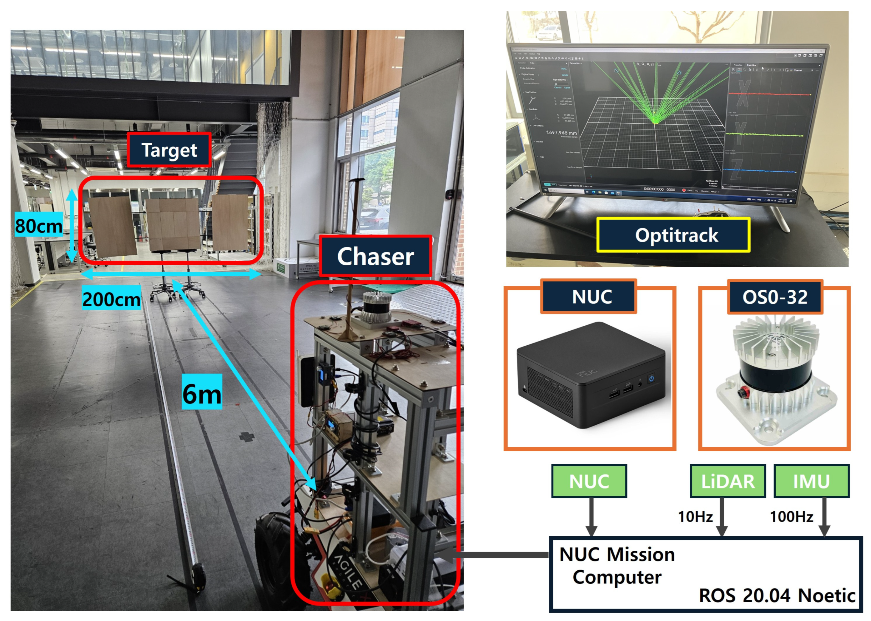
5.1. Experiment Environment

Since the simulation data do not perfectly simulate the data from the actual sensor, an experimental environment was constructed to generate real data and verify the algorithm. The Ouster LiDAR sensor simulation was used, and the IMU data were used as the IMU embedded in the LiDAR. In addition, the shape of the actual satellite model was created and used as the target, and the chaser was used as a UGV. The experimental environment was configured as shown in Figure 8.

The left side of Figure 8 shows the close docking scenario of the target and chaser in the indoor experiment. The target is a simple satellite with dimensions 200 cm in width and 80 cm in height, while the chaser, a UGV(WeGo), is equipped with sensors and a mission computer called NUC(Intel), and the target and chaser are positioned 6 m apart. The UGV slowly approached the target with very slow, straight-line driving, IMU was stored in the NUC at 100 Hz, and point cloud data were stored at 10 Hz through Ouster LiDAR. An optical precision positioning device called Optitrack was used as the reference device, and both sensor data and reference data were stored through ROS 20.04 on the NUC.

Table 3. LiDAR sensor specification in the experiment.

LiDAR Sensor	OS0–32
Maximum range	0.5 m
Minimum range	50 m
Vertical Resolution	32
Horizontal Resolution	1024
Field of View	Horizontal: 360° Vertical: −45°~45°

shows the specifications of the LiDAR sensor used in the actual experiment.

5.2. Experiment Result

Similarly, we compared the performance of algorithms through experiments. Like in Section 4.2, we first compare the variance and eigenvector variation in the covariance matrix of the point clouds.

Figure 9 shows the variance and eigenvectors of the covariance matrix for the satellite designed for the real experiment in Figure 8. Unlike the simulation, the real data from the LiDAR show that the variance and eigenvectors change frequently. Unlike the simulation, the actual experiment was conducted at a reduced scale, so the size of the target is relatively small, and the LiDAR sensor is different from the simulation; thus, the distribution of point cloud data changes significantly with distance, as shown in Figure 10. Not only the density of the point clouds but also the vertical axis distribution of the point clouds according to the distance is changed by the resolution of the vertical axis of LiDAR, and the variance of the covariance and the eigenvectors change significantly when applying the PCA method.

The following shows the variance and eigenvector of point cloud data using the E2PCA method.

Like the simulation, the point cloud obtained from the experiment shows very small changes in variance and eigenvectors in Figure 11. This shows that the E2PCA method can be applied to obtain a stable initial rotation matrix even if the density and distribution of the point cloud data change frequently. Similarly to the simulation, error-state EKF was applied to compare the position and attitude error estimation results for each algorithm. For each method, we performed propagation using the INS model and then combined the EKF filter using the measurements obtained by each algorithm.

First, we compared the initial attitude results for each algorithm and the overall attitude estimation results to be used as a measurement for the EKF.

As shown in Figure 12a, the E2PCA method proposed in this paper has the most stable initial attitude results, and when the measurements are calculated based on the initial value, E2PCA-CMT has the best estimation results, as shown in Figure 12b.

Table 4. Algorithm attitude estimation RMSE in the experiment.

Algorithm	Attitude RMSE (deg)
	Roll	Pitch	Yaw
ICP	3.0079	1.0836	0.4075
PCA-CMT	0.4400	1.4324	1.8030
E2PCA-CMT	0.7755	0.9009	0.8739

below shows the RMSE of attitude estimation results for each algorithm.

The navigation results for each algorithm of the EKF combined with the INS model using the attitude estimation results as a measurement are shown in Figure 13.

The experimental results also show that the E2PCA-CMT method has the best overall estimation results for position and attitude estimation. In the case of the ICP algorithm, similar to the simulation, it can be seen that the error is large in the initial section that is not properly matched, and then the estimation becomes stable. In the case of E2PCA-CMT, the roll and pitch attitude estimation show a significant reduction in error compared to the other two methods. However, in the case of position, we can see that the estimation error is relatively large compared to the simulation. As shown in Figure 14, the scale of the target is reduced in the actual experimental environment, unlike the simulation, and the vertical axis resolution of the LiDAR causes an error in position estimation based on the center point of the point cloud, which is characteristic of the CMT algorithm.

As shown in Figure 14, the center point of the point cloud in the real experiment changes as the distance decreases, and, as shown in Figure 13, a location error occurs due to the change in the center point.

Table 5. Algorithm pose estimation RMSE in the experiment.

Algorithm	Position RMSE (m)			Attitude RMSE (deg)
	East	North	Up	Roll	Pitch	Yaw
INS/ICP EKF	0.0538	0.0386	0.3738	2.9988	1.0878	0.3847
INS/PCA-CMT EKF	0.1123	0.0523	0.0620	0.7746	1.6721	1.0015
INS/E2PCA-CMT EKF	0.1043	0.0550	0.0556	0.3445	0.7485	1.0163

shows the RMSE of each algorithm for the real experimental results.

6. Discussion

6.1. Performance Analysis of Algorithms Based on Point Cloud Estimation Results

In this study, we studied a LiDAR point cloud data processing algorithm for accurate pose estimation for a straight-approach scenario with no attitude change in a space environment. The main technology of the proposed method is the combination of ICP and the PCA method to minimize the pose estimation error, which results in more accurate navigation estimation than the existing general methods. The simulation and experimental results in Section 4.2 and Section 5.2 show that the algorithm proposed is improved in position and attitude. In addition, the simulation results reflecting the actual scale using the ISS model showed relatively better navigation performance than the actual experimental results, which indicates that if the experiments use point cloud data through a more precise and large-scale target model, better navigation results can be shown in actual experiments.

6.2. Loosely Coupled EKF Filter Design Based on Measurements and the INS Model

As shown in the structure in Figure 3, the algorithm proposed in this paper is a Loosely Coupled EKF filter that uses the position and attitude calculated by the point cloud pose estimation as measurements. The accuracy of the measurements is the most important part of the Loosely Coupled filter to solve the shortcomings of the INS model, which accumulates errors over time. Therefore, we used the CMT algorithm to improve the accuracy of the measurements and compared it with the simulation and experiments.

In the experimental environment, the model size and shape of the target, sensor specification, experimental time, and scenario distance were important factors. Unlike the simulation, the experimental results showed that the error of position was relatively large for both ICP and E2PCA-CMT. This result is because the distribution and density of point clouds are significantly changed by the specification of sensors, as shown in Figure 10. The size and density of data vary depending on the vertical FOV (Field of View) and resolution of the LiDAR sensor. Since the target model designed in the experiment was small compared to the performance of the LiDAR we used, it was not enough to acquire enough point clouds in all sections, which resulted in a relatively large change in the center point of data used for position estimation, as shown in Figure 14. For this reason, researchers are increasingly using TOF cameras to acquire point cloud data instead of LiDAR in space environments, and it is still an important issue to determine the performance of LiDAR in space and develop algorithms that can perform precise estimation even in poor environments. This indicates the need for a Tightly Coupled filter design that is robust to the performance of LiDAR using raw data, and at the same time provides a direction for improvement in this study.

6.3. Analysis of the Real-Time and Practical Application of Algorithms

Ensuring the real-time performance of the algorithm is one of the important factors in actual space missions.. While research on accurate navigation algorithms is ongoing, ensuring both computational efficiency and real-time navigation performance of the algorithm remains a challenging task. The algorithm proposed in this paper also has limitations in real-time performance. To compare the computational speed of the algorithm, we used MATLAB’s profiler function to compare the speed of computation.

Table 6. Computer specifications used to measure the real time of the algorithm.

PC Specification	System
Processor	13th Intel® Core i5-13600KF 3.50 GHz
Installed RAM	64.0 GB DDR5
Operating system	Window 11, 64 bits
Graphics	NVIDIA GeForce RTX 4070 Ti
MATLAB version	MATLAB R2023b

summarizes the specifications of the PC used to apply the data obtained through simulation and experiment to the algorithms. The computational speeds of ICP, PCA, and CMT were calculated on the PC with the corresponding specifications to analyze the real-time performance.

The computation time for each method calculated by simulation and experiments is shown in

Table 7. Computing time of algorithm in the simulation and experiment.

Algorithm	Simulation		Experiment
	Total Time	Data Number	Total Time	Data Number
ICP	61.025 s	925 × 10 Hz and 20,000 point	6.47 s	1324 × 10 Hz and 1000 point
E2PCA	104.621 s		7.488 s
E2PCA-CMT	222.267 s		13.97 s

above. Both simulation and experiment results show that E2PCA and CMT together took longer processing times than ICP alone. In the case of the experiment, about 1000-point cloud data every 0.1 s for a total of 132.4 s were calculated, and the algorithm ran very fast in this case. On the other hand, the simulation processed about 20,000-point cloud data every 0.1 s for a total of 92.5 s, and the computational speed increased by 10~20 times for each algorithm compared to the experiment. This shows that the size of the point cloud data has a significant influence on the computational speed.

Since the target model in the experiment is not the actual ISS and the size of the point cloud data is small, the algorithm speed of the simulation can indirectly provide an indication of real-time performance. When using ICP alone, it took 61.025 s to process a total of 925 s of data, so it is possible to implement a real-time algorithm up to 15 Hz. However, if E2PCA is used, it can be implemented at around 11 Hz, and if E2PCA-CMT, which is proposed in this paper, is used, the real-time performance drops to 4.16 Hz. Since the computation time in this paper is calculated based on the PC specifications in Table 6, the real-time performance is more likely to decrease if a lower PC is used.

In future research, it is necessary to effectively reduce the point cloud data using a voxel filter to ensure real-time performance. The current algorithm uses all the acquired point data, but if an appropriate voxel size is used, the number of points can be reduced while maintaining the distribution of the entire point cloud, resulting in more faster computation.

7. Conclusions

In this paper, we propose a pose estimation algorithm based on relative navigation for scenarios with small pose changes during close-range cooperative rendezvous/docking. Principal component analysis (PCA) was applied to the covariance matrix of the point cloud data, and the distribution and eigenvectors of the point cloud data were calculated by ICP matching. The attitude transformation matrix calculated from the eigenvectors was used to calculate the rotation matrix between consecutive frames, which was used as an initial value to apply to the CMT algorithm. In addition, an INS model was designed and combined with the point cloud algorithm to design a combined INS/LiDAR filter for the space environment, and the algorithm was verified through simulation and experiments. The simulation results showed that the performance of the algorithm proposed in the paper was within a 0.05 m position error and 0.03° attitude error, while the experimental results showed a position error within 0.1 m and attitude error within 1°. Both results show that the overall position and attitude estimation performance is better than the existing algorithms, and as a result, the algorithm proposed in this paper is capable of performing rendezvous/docking scenarios. However, as mentioned in the experimental results, navigation errors can occur depending on the specifications of the LiDAR sensor. These results demonstrate the limitations of using measurements based on point cloud estimation but also the need for a Tightly Coupled filter design using raw point cloud data that is robust to sensor specifications and the direction of future research.

References

1. Du, X.; He, Y.; Chen, L.; Gao, S. Pose estimation of large non-cooperative spacecraft based on extended PnP model. In Proceedings of the 2016 IEEE International Conference on Robotics and Biomimetics (ROBIO), Qingdao, China, 3–7 December 2016; IEEE: Piscataway, NJ, USA, 2016; pp. 413–418. [Google Scholar]
2. Du, X.; Liang, B.; Xu, W.; Qiu, Y. Pose measurement of large non-cooperative satellite based on collaborative cameras. Acta Astronaut. 2011, 68, 2047–2065. [Google Scholar]
3. Opromolla, R.; Fasano, G.; Rufino, G.; Grassi, M. A review of cooperative and uncooperative spacecraft pose determination techniques for close-proximity operations. Prog. Aerosp. Sci. 2017, 93, 53–72. [Google Scholar] [CrossRef]
4. Bezouska, W.; Barnhart, D. Decentralized cooperative localization with relative pose estimation for a spacecraft swarm. In Proceedings of the 2019 IEEE Aerospace Conference, Big Sky, MT, USA, 2–9 March 2019; IEEE: Piscataway, NJ, USA, 2019; pp. 1–13. [Google Scholar]
5. Martínez, H.G.; Giorgi, G.; Eissfeller, B. Pose estimation and tracking of non-cooperative rocket bodies using time-of-flight cameras. Acta Astronaut. 2017, 139, 165–175. [Google Scholar] [CrossRef]
6. Perfetto, D.M.; Opromolla, R.; Grassi, M.; Schmitt, C. LIDAR-based model reconstruction for spacecraft pose determination. In Proceedings of the 2019 IEEE 5th International Workshop on Metrology for AeroSpace (MetroAeroSpace), Turin, Italy, 19–21 June 2019; IEEE: Piscataway, NJ, USA, 2019; pp. 1–6. [Google Scholar]
7. Mark, C.P.; Kamath, S. Review of active space debris removal methods. Space Policy 2019, 47, 194–206. [Google Scholar] [CrossRef]
8. Woods, J.O.; Christian, J.A. Lidar-based relative navigation with respect to non-cooperative objects. Acta Astronaut. 2016, 126, 298–311. [Google Scholar]
9. He, Y.; Liang, B.; He, J.; Li, S. Non-cooperative spacecraft pose tracking based on point cloud feature. Acta Astronaut. 2017, 139, 213–221. [Google Scholar]
10. He, Y.; Yang, J.; Xiao, K.; Sun, C.; Chen, J. Pose tracking of spacecraft based on point cloud DCA features. IEEE Sens. J. 2022, 22, 5834–5843. [Google Scholar]
11. Li, P.; Wang, M.; Zhou, D.; Lei, W. A pose measurement method of a non-cooperative spacecraft based on point cloud feature. In Proceedings of the 2020 Chinese Control and Decision Conference (CCDC), Hefei, China, 22–24 August 2020; IEEE: Piscataway, NJ, USA, 2020; pp. 4977–4982. [Google Scholar]
12. Chen, Z.; Li, L.; Niu, K.; Wu, Y.; Hua, B. Pose measurement of non-cooperative spacecraft based on point cloud. In Proceedings of the 2018 IEEE CSAA Guidance, Navigation and Control Conference (CGNCC), Xiamen, China, 10–12 August 2018; IEEE: Piscataway, NJ, USA, 2018; pp. 1–6. [Google Scholar]
13. Opromolla, R.; Fasano, G.; Rufino, G.; Grassi, M. Pose estimation for spacecraft relative navigation using model-based algorithms. IEEE Trans. Aerosp. Electron. Syst. 2017, 53, 431–447. [Google Scholar] [CrossRef]
14. Yuan, C.; Yu, X.; Luo, Z. 3D point cloud matching based on principal component analysis and iterative closest point algorithm. In Proceedings of the 2016 International Conference on Audio, Language and Image Processing (ICALIP), Shanghai, China, 11–12 July 2016; IEEE: Piscataway, NJ, USA, 2016; pp. 404–408. [Google Scholar]
15. Zhang, G.; Huo, J.; Zhang, Z.; He, M.; Zhang, J.; Xue, M. Novel pose measurement with optimized principal component analysis for unknown spacecraft based on point cloud. In Proceedings of the 5th International Conference on Multimedia and Image Processing, Nanjing, China, 10–12 January 2020; pp. 102–108. [Google Scholar]
16. Besl, P.J.; McKay, N.D. Method for registration of 3-D shapes. In Proceedings of the Sensor Fusion IV: Control Paradigms and Data Structures, Boston, MA, USA, 12–15 November 1992; Volume 1611, pp. 586–606. [Google Scholar]
17. Kang, G.; Zhang, Q.; Wu, J.; Zhang, H. Pose estimation of a non-cooperative spacecraft without the detection and recognition of point cloud features. Acta Astronaut. 2021, 179, 569–580. [Google Scholar]
18. Gavin, H.P. The Levenberg-Marquardt Algorithm for Nonlinear Least Squares Curve-Fitting Problems; Department of Civil and Environmental Engineering, Duke University: Durham, NC, USA, 2019; Volume 3. [Google Scholar]
Figure 1. Example of a point cloud eigenvector using the PCA method.
Remotesensing 17 01091 g001
Figure 2. Distribution of point cloud based on distance and ICP registration: (a) 30 m ISS point cloud; (b) docking distance (2 m) ISS point cloud; (c) 30 m ISS point cloud using ICP; (d) docking distance (2 m) ISS point cloud using ICP.
Remotesensing 17 01091 g002
Figure 3. INS/LiDAR error-state Extended Kalman Filter structure.
Remotesensing 17 01091 g003
Figure 4. INS/LiDAR filter algorithm configuration using Gazebo simulation.
Remotesensing 17 01091 g004
Figure 5. Variance and eigenvector variation result of PCA in simulation: (a) variance change in point cloud; (b) first eigenvector direction change; (c) second eigenvector direction change; (d) third eigenvector direction change.
Remotesensing 17 01091 g005
Figure 6. Variance and eigenvector variation result of E2PCA in simulation: (a) variance change in point cloud; (b) first eigenvector direction change; (c) second eigenvector direction change; (d) third eigenvector direction change.
Remotesensing 17 01091 g006
Figure 7. Error-state extended Kalman filter pose estimation result in simulation: (a) relative position error; (b) relative attitude error.
Remotesensing 17 01091 g007
Figure 8. Configuration of experimental environment.
Remotesensing 17 01091 g008
Figure 9. Variance and eigenvector variation result of PCA in the experiment: (a) variance change in point cloud; (b) first eigenvector direction change; (c) second eigenvector direction change; (d) third eigenvector direction change.
Remotesensing 17 01091 g009
Figure 10. Point cloud distribution of target model by distance in experiment: (a) initial point cloud at a 6m distance; (b) final point cloud at a 1m distance.
Remotesensing 17 01091 g010
Figure 11. Variance and eigenvector variation result of E2PCA in experiment: (a) variance change in point cloud; (b) first eigenvector direction change; (c) second eigenvector direction change; (d) third eigenvector direction change.
Remotesensing 17 01091 g011
Figure 12. Estimation result in experiment: (a) initial attitude error; (b) relative attitude error.
Remotesensing 17 01091 g012
Figure 13. Error-state extended Kalman filter pose estimation result in experiment: (a) relative position error; (b) relative attitude error.
Remotesensing 17 01091 g013
Figure 14. Change in the center point in the experiment.
Remotesensing 17 01091 g014