Article

Projecting Future Wetland Dynamics Under Climate Change and Land Use Pressure: A Machine Learning Approach Using Remote Sensing and Markov Chain Modeling

1
College of Science, Inner Mongolia Agricultural University, Hohhot 010018, China
2
National Orientation Observation and Research Station of Saihanwula Forest Ecosystem in Inner Mongolia, Daban, Chifeng 025000, China
3
College of Forestry, Inner Mongolia Agricultural University, Hohhot 010018, China
4
School of Geography, Development and Environment, The University of Arizona, Tucson, AZ 85719, USA
5
Inner Mongolia Forestry and Grassland Monitoring and Planning Institute, Hohhot 010020, China
6
Key Laboratory of Digital Earth Science, Aerospace Information Research Institute, Chinese Academy of Sciences, Beijing 100094, China
7
Institute of Remote Sensing Satellite, China Academy of Space Technology, Beijing 100095, China
*
Author to whom correspondence should be addressed.
These authors contributed equally to this work.
Remote Sens. 2025, 17(6), 1089; https://doi.org/10.3390/rs17061089
Submission received: 19 January 2025 / Revised: 14 March 2025 / Accepted: 17 March 2025 / Published: 20 March 2025
(This article belongs to the Special Issue Application of Remote Sensing Technology in Wetland Ecology)

Abstract

:
Wetlands in the Yellow River Watershed of Inner Mongolia face significant reductions under future climate and land use scenarios, threatening vital ecosystem services and water security. This study employs high-resolution projections from NASA’s Global Daily Downscaled Projections (GDDP) and the Intergovernmental Panel on Climate Change Sixth Assessment Report (IPCC AR6), combined with a machine learning and Cellular Automata–Markov (CA–Markov) framework to forecast the land cover transitions to 2040. Statistically downscaled temperature and precipitation data for two Shared Socioeconomic Pathways (SSP2-4.5 and SSP5-8.5) are integrated with satellite-based land cover (Landsat, Sentinel-1) from 2007 and 2023, achieving a high classification accuracy (over 85% overall, Kappa > 0.8). A Maximum Entropy (MaxEnt) analysis indicates that rising temperatures, increased precipitation variability, and urban–agricultural expansion will exacerbate hydrological stress, driving substantial wetland contraction. Although certain areas may retain or slightly expand their wetlands, the dominant trend underscores the urgency of spatially targeted conservation. By synthesizing downscaled climate data, multi-temporal land cover transitions, and ecological modeling, this study provides high-resolution insights for adaptive water resource planning and wetland management in ecologically sensitive regions.

1. Introduction

Wetlands are vital ecosystems that play a fundamental role in maintaining ecological balance, supporting biodiversity, and delivering essential ecosystem services such as water purification, flood regulation, and carbon sequestration [1]. These ecosystems provide habitats for a wide array of species and are integral to the health of the surrounding environments. However, they are increasingly threatened by the combined pressures of climate change and human-induced land use alterations [2]. The Yellow River Watershed in Inner Mongolia represents one of the most ecologically sensitive regions in China, where the protection and sustainable management of wetlands have become critical due to their essential role in regional biodiversity, water regulation, and local livelihoods [3]. Understanding the future dynamics of these aquatic ecosystems under combined environmental pressures is vital for effective conservation and sustainable land use planning [4].
Climate change directly threatens wetlands by altering hydrological cycles, precipitation patterns, and the frequency of extreme weather events [5]. Changes in temperature and precipitation can lead to changes in water levels, affecting these ecosystems’ ecological integrity and functionality [6]. Simultaneously, land use changes, including agricultural expansion, urban development, and infrastructure construction, place additional pressures on wetlands [7]. These combined forces disturb natural hydrological processes, change soil and water properties, and threaten the biodiversity of aquatic habitats [8]. Addressing these challenges requires the development of predictive models that can simulate the future dynamics of wetlands under multiple environmental stressors [9]. This need is particularly acute in regions like the Yellow River Watershed, where ecological sensitivity and socioeconomic significance heighten the need for accurate and localized predictions [10,11].
Researchers increasingly rely on advanced computational and geospatial techniques to address the combined pressures of climate change and land use transformations. Such methods help to capture the complex interplay among temperature shifts, precipitation variability, and land cover dynamics and enable the robust predictions of ecosystem responses. Recent advances in remote sensing (RS) and machine learning (ML) have facilitated the analysis of changes in aquatic ecosystems with enhanced precision and scalability [12,13]. Remote sensing offers large-scale, multi-temporal datasets that provide detailed spatial and temporal insights into changes in wetlands [14,15]. Concurrently, machine learning algorithms, such as Random Forest (RF), Support Vector Machines (SVM), and Gradient Boosting (GB), enable the detection of complex, non-linear relationships in geospatial data [16]. Traditional models for land cover change often fail to account for the probabilistic nature of transitions in land use, which is why Markov Chain models have emerged as critical tools. These models predict the likelihood of future land cover changes by analyzing historical trends [17]. When combined with machine learning techniques, Markov Chain models enhance predictive power, offering a more robust approach to forecasting land cover and the dynamics of wetlands.
Despite these advancements, substantial knowledge gaps remain. Current predictive models often fail to address the localized effects of climate change and land use pressures, particularly in regions like the Yellow River Watershed. Moreover, many models rely on coarse-resolution climate data, which limits the granularity and precision of predictions. To address these gaps, this study introduces an innovative modeling framework that integrates high-resolution climate projections from NASA’s GDDP and IPCC AR6 models with a hybrid machine learning–Markov Chain model. In addition, by leveraging the capabilities of the Google Earth Engine, NASA’s GDDP datasets are statistically downscaled to the TerraClimate dataset [18], enhancing the spatial precision of the outputs. This approach provides a more detailed analysis of the dynamics of wetlands at the regional level and introduces methodological enhancements that improve prediction accuracy.
The proposed framework has three primary components: First, high-resolution climate projections are generated using NASA’s GDDP and IPCC’s AR6 models [19]. These projections capture potential changes in precipitation, temperature, and extreme weather events, critical for predicting hydrological changes affecting wetlands. Second, land use and land cover changes are modeled using the Markov Chain and CA–Markov models implemented within the TerrSet 2020 software. These models leverage spatial simulation and analysis techniques to accurately model land cover transitions and predict future patterns of change. The CA–Markov model utilizes historical land cover data to simulate and predict future changes. By integrating the predictive capability of cellular automata with a Markov-Chain-based transition probability matrix, the model effectively captures the spatial and stochastic nature of land use transitions, thereby enhancing the accuracy of predictions. Third, the MaxEnt model is employed to generate a habitat suitability map for wetlands. Using future climate variables and projected land use data, the MaxEnt model predicts the probability of wetland presence, providing a detailed assessment of potential wetland distribution under changing environmental conditions. This comprehensive framework provides a site-specific analysis of wetland and water body dynamics in the Yellow River Watershed. By integrating climate, land use, and ecological modeling, it addresses the gaps in previous studies.
The main objectives of this study are as follows:
  • To project future climate conditions under SSP (Shared Socioeconomic Pathway) scenarios.
  • To use advanced modeling techniques to predict future land use and land cover changes, explicitly focusing on wetland areas.
  • To forecast future changes in the distribution of wetlands under different climate change and land use pressure scenarios.
  • To provide actionable insights for conservation planning and the sustainable management of aquatic ecosystems by offering accurate, high-resolution predictions for policymakers and stakeholders.
This study contributes to the growing knowledge on the resilience and adaptive management of wetlands under environmental change. The novel hybrid modeling framework proposed here addresses gaps in predictive precision by incorporating region-specific climate projections and advanced predictive algorithms. The results are expected to support evidence-based decision-making, inform conservation policy, and provide valuable insights for stakeholders aiming to preserve aquatic ecosystems amid ongoing environmental pressures.

2. Materials and Methods

2.1. Study Area

The Inner Mongolia section of the Yellow River Watershed is situated in the middle and upper reaches of the Yellow River Basin. This region is defined by geographic coordinates: 42°44′11.23″N at its northernmost point, 37°37′15.61″N at its southernmost point, 105°11′51.07″E at its westernmost point, and 112°18′17.30″E at its easternmost point. Covering a total area of approximately 198,403.6 km2, this section accounts for a significant portion of the watershed, characterized by diverse topographical and ecological features [20]. The elevation within the region ranges from 796 m to 2336 m above sea level, encompassing a variety of landscapes, including alluvial plains, plateaus, mountains, hills, deserts, and lakes. This diversity supports a rich array of vegetation and ecosystems. Prominent geographical features include the Ulanbuhe Desert, the Hetao Irrigation District, the Tumochuan Plain, and the Kubuqi Desert. The Yellow River traverses this region over approximately 830 km, passing through key administrative areas such as Hohhot, Baotou, Wuhai, Ordos, Bayannur, Alashan, and Ulanqab [21]. The region experiences an average annual temperature of 6.7 °C and annual precipitation ranging from 120 to 420 mm, reflecting the semi-arid to arid climate typical of Inner Mongolia [21]. These climatic conditions and this diverse topography create a mosaic of ecological zones with distinct functional attributes [20]. This section of the Yellow River Watershed plays a vital role in balancing agricultural, urban, and ecological needs, making it a focal area for studying the impacts of climate change, land use pressures, and water resource management [20] (Figure 1).

2.2. Data Sources

2.2.1. Satellite-Based Remote Sensing Data

Satellite imagery was used to analyze the optical and radar signatures of the Earth’s surface. For the optical domain, data from Landsat 8 (Collection 2 Surface Reflectance) and Landsat 5 (Collection 2 Top of Atmosphere) were employed to compute a range of spectral indices, including the Normalized Difference Vegetation Index (NDVI), Normalized Difference Water Index (NDWI), and Normalized Difference Tillage Index (NDTI). These indices were calculated for distinct periods—2023 for Landsat 8 and 2007 for Landsat 5—to facilitate the assessment of temporal changes in vegetation and land surface properties. Complementing this, radar data from Sentinel-1 Ground Range Detected (GRD) imagery, specifically VV and VH polarizations, were processed to derive features such as VV+VH, VV–VH, their ratio, and their mean values. This integrated approach combining optical and radar datasets offered a robust framework for land cover classification, leveraging backscatter sensitivity to surface roughness and moisture in conjunction with the spectral reflectance properties critical for distinguishing various land cover types (Table 1).

Remote Sensing Preprocessing (Landsat and Sentinel-1)

Landsat Data: Level-2 Surface Reflectance products (Landsat 8 for 2023 and Landsat 5 for 2007) were acquired through the Google Earth Engine (GEE) to ensure atmospheric and radiometric corrections were already applied. Additional quality assurance (QA) filtering included cloud and shadow masking based on bitmask flags. Spectral indices such as the Normalized Difference Vegetation Index (NDVI) and the Normalized Difference Water Index (NDWI) were computed on cloud-free composites to capture key land cover signatures.
Sentinel-1 Data: Radar images were obtained in interferometric-wide (IW) mode with VV and VH polarizations. The preprocessing steps included radiometric calibration, thermal noise removal, and terrain correction, all handled via GEE’s built-in workflows. Multi-temporal speckle reduction was also applied to minimize noise. These steps collectively ensured that the backscatter values accurately represented land surface conditions, particularly differentiating open water from partially inundated or vegetated surfaces.

2.2.2. Topographic Data

To quantify terrain variability, the NASADEM dataset (NASADEM_HGT/001) [22] was utilized to extract elevation data with a spatial resolution of approximately 30 m. Using these elevation values, key terrain attributes, including aspect and slope, were derived through standard digital terrain analysis techniques. Additionally, a global landform product based on the SRTM dataset [23] was incorporated to classify the Earth’s surface into distinct geomorphological categories. These topographic variables are essential for various spatial analyses, as they significantly influence environmental factors such as the microclimate and hydrological processes [24]. When integrated into land cover or habitat suitability models, these variables contribute to enhanced model accuracy and reliability (Table 1).
This study relied on Sentinel-1 C-band SAR (VV and VH polarizations) primarily due to its global coverage, frequent revisit cycle, and seamless integration with the Google Earth Engine. While L-band SAR (e.g., from ALOS PALSAR) can penetrate dense canopies more effectively and thus enhances forest monitoring, its availability in the Google Earth Engine remains limited regarding both temporal span and spatial coverage. In this analysis, the incorporation of Sentinel-1 data, together with optical indices (e.g., NDVI) and topographic variables, proved sufficient for the robust discrimination of vegetation classes, including forests. Future research could explore L-band SAR as a feasible complementary data source, particularly for in-depth forest assessments requiring greater sensitivity to vertical canopy structure. The current classification strategy, however, demonstrated a high accuracy and effectively captured the broader land cover dynamics under both natural and anthropogenic pressures.

2.2.3. Soil Data

Soil characteristics are fundamental in shaping vegetation patterns, hydrological dynamics, and overall ecosystem functionality [25]. To capture this variability, USDA soil texture classes were extracted from the OpenLandMap Soil Texture dataset [26], which provided a 250 m resolution map of soil texture categories, ranging from coarse sands to heavier clay soils. Incorporating these data enabled the study to account for edaphic factors that influence land cover distribution, agricultural suitability, and species’ habitat preferences. This information was particularly valuable for ecological modeling, flood risk assessments, and land management strategies aimed at optimizing productivity while promoting environmental sustainability [27] (Table 1).

2.2.4. Climate Data

Current and projected climate variables were incorporated to analyze baseline conditions and potential future scenarios. TerraClimate data [18] served as the primary sources for baseline and annual climate parameters, including precipitation (pr), minimum and maximum temperatures (tmmn, tmmx), and solar radiation (srad). These datasets, available at an approximately 4 km spatial resolution, were processed to calculate aggregate or mean values, such as annual precipitation and mean annual temperature. NASA/GDDP-CMIP6 data [19] were utilized to evaluate the potential impacts of climate change. This dataset provides downscaled climate projections from CMIP6 GCM runs, supporting the IPCC AR6 assessment. The analysis was conducted under two representative scenarios: SSP2-4.5 (moderate emissions) and SSP5-8.5 (high emissions) [28]. Multi-model means, derived by averaging the outputs from several global climate models, enabled robust comparisons between historical (1985–2015) and future (2030–2050) temperature and precipitation regimes (Table 1).

2.2.5. Data Integration and Temporal Alignment

To ensure consistency across multiple datasets and facilitate climate projections through 2040, this study adopted a common reference baseline (1985–2015) for climate data while employing single-year land cover snapshots from 2007 and 2023. These specific years capture distinct temporal conditions and serve as anchors for modeling land cover transitions. The 2019 land cover dataset was also incorporated to refine the classification schemes and validate the spatial patterns, enriching our understanding of local land use dynamics. Sentinel-1 radar imagery was only available from 2014 onwards; thus, it was exclusively integrated with the optical data (Landsat) from 2023, enhancing classification accuracy through a complementary data fusion approach. The year 2007 was selected to establish a long-term baseline, providing an essential historical reference for the robust modeling of land use transitions spanning approximately two decades. In contrast, datasets such as NASADEM, landforms (SRTM-based), and OpenLandMap Soil Texture were treated as static inputs; their core characteristics (elevation, geomorphological features, and soil properties) were assumed to remain effectively unchanged over the study period and were accessed via the Google Earth Engine. This integrated approach ensured an alignment in spatial resolution and reference periods, thereby preserving the unique strengths of each dataset while minimizing potential inconsistencies in land cover and climate analyses (Table 1).
Table 1. Summary of datasets used.
No.Dataset NameSpatial ResolutionTemporal CoverageKey Variables/BandsPurposeSource (Reference)
1Copernicus Global Land Cover (2019)100 m2019discrete_classificationLand cover mapping and reference for classification[29]
2Sentinel-1 (GRD)~10 m1 January 2023–1 January 2024Radar bands VV, VH + derived indicesExtraction of radar backscatter features (VV, VH, and indices) for land use/cover classification[30]
3Landsat 8 C2 SR30 m1 January 2023–1 January 2024Reflective bands (B2-B7), NDVI, NDWI, NDTICalculation of spectral indices and time-series composites for land cover classification[31]
4Landsat 5 C2 SR30 m1 January 2007–1 January 2008Reflective bands (B1-B6), NDVI, NDWI, NDTIHistorical assessment of land surface conditions and spectral indices[32]
5NASADEM~30 m-ElevationExtraction of topographic variables: elevation, slope, aspect[22]
6Landforms (SRTM-based)90 m-Constant (landforms)Characterization of geomorphological landforms[23]
7OpenLandMap Soil Texture250 m-b0USDA texture classification of soils[26]
8TerraClimate~4 km1985–2015 (baseline) and 2023pr, tmmn, tmmx, sradBaseline and annual climate variables (precipitation, temperature, radiation)[18]
9NASA/GDDP-CMIP6~0.25° (~25 km)1985–2015/2030–2050tas, pr (under scenarios SSP2-4.5, SSP5-8.5)Future climate projections (temperature and precipitation changes)[19]

2.3. Future Climate Projection and Downscaling

This section describes the methodology for generating, evaluating, and downscaling future climate scenarios in the study region. The workflow consisted of three main steps: (i) selecting a set of General Circulation Models (GCMs) with a robust performance over China based on Taylor diagram analysis; (ii) applying a multi-model mean approach to analyze temperature and precipitation projections under two Shared Socioeconomic Pathways (SSP2-4.5 and SSP5-8.5) for the period 2030–2050; and (iii) employing a statistical downscaling method within the Google Earth Engine (GEE) to downscale the climate data spatially. The visualization of climate trends and model performance was performed using Google Colab, including the generation of Taylor diagrams.

2.3.1. Model Selection via Taylor Diagrams

Initially, six models demonstrating strong performance over China were selected based on a comprehensive review of the scientific literature [33,34,35,36]. These models included ACCESS-CM2, CNRM-CM6-1, CNRM-ESM2-1, MPI-ESM1-2-HR, MRI-ESM2-0, and UKESM1-0-LL. Their historical performance during the baseline (1985–2015) was evaluated using observed climate data as the reference. Key statistical metrics were calculated to assess model performance, including Pearson’s correlation coefficients (Equation (1)) and normalized standard deviations. These metrics were visually summarized in a Taylor diagram, which comprehensively represented each model’s spatial and temporal agreement with the reference data.
The Taylor diagram is a widely used tool for evaluating and comparing the performance of multiple models across various dimensions [37]. It offers a concise visual summary of how well the models align with observations, incorporating factors such as the standard deviation of the model time-series and the correlation between the observed and modeled values. The Taylor diagram provides a robust framework for assessing model performance by integrating metrics like the Pearson correlation coefficient and the standard deviation. Models with high correlations and near-unity standard deviation ratios were selected for inclusion in the multi-model ensemble used in subsequent analyses [38].
r = i = 1 n x i x ¯ y i y ¯ i = 1 n x i x ¯ 2 × i = 1 n y i y ¯ 2
where xi and yi represent the model and the observed values, x ¯ and y ¯ are their respective means, and n is the total number of observations [39].

2.3.2. Multi-Model Mean and Scenarios (2030–2050)

The selected ensemble of General Circulation Models (GCMs) provided outputs for two key climate variables: near-surface temperature and precipitation, under two scenarios—SSP2-4.5 (moderate emissions) and SSP5-8.5 (high emissions). Historical data (1985–2015) and future projections (2030–2050) were retrieved from the NASA/GDDP-CMIP6 collection in the Google Earth Engine (GEE). For temperature, the change (ΔT) for each model was calculated as follows [40,41]:
Δ T = T f u t u r e T b a s e l i n e
where Tfuture represents the mean temperature during the future period (2030–2050), and Tbaseline is the mean temperature during the baseline period (1985–2015).
The ensemble-mean temperature change (ΔTMMM) was then derived by averaging the individual temperature changes (ΔT) across all selected models:
Δ T M M M = i = 1 m Δ T i m
where m is the total number of models in the ensemble, and ΔTi is the temperature change for the i-th model.
For precipitation, a ratio-based approach was used to capture percentage changes. The precipitation change factor (Pchange) for each model was computed as:
P c h a n g e = P f u t u r e P b a s e l i n e
where Pfuture and Pbaseline denote the mean precipitation during the future and baseline periods, respectively.
The multi-model mean precipitation change (PMMM) was calculated by averaging the precipitation change factors across all models:
P M M M = i = 1 m P c h a n g e , i m
where Pchange,i is the precipitation change factor for the i-th model.
These ensemble-mean changes in temperature and precipitation provided a robust basis for understanding potential climate shifts under the specified scenarios. Combining the outputs from multiple models reduced uncertainty and ensured more reliable projections for the study area [42,43,44].

2.3.3. Statistical Downscaling in the Google Earth Engine

The statistical downscaling method [45,46] establishes relationships between observed climate data and large-scale predicted data from climate models. This process involves evaluating the model’s performance by comparing observed data with historical projections from General Circulation Models (GCMs) and applying bias correction to enhance the accuracy of future climate projections. In this study, NASA’s GDDP data were statistically downscaled to TerraClimate data within the Google Earth Engine environment, thereby improving the spatial resolution of the resulting climate datasets. This method adjusted baseline climate data using projected ensemble-mean changes while preserving the spatial and temporal patterns of the original high-resolution data [47].

Future Adjusted Temperature (Tadj)

The adjusted temperature for future scenarios (Tadj) is computed by adding the ensemble-mean temperature change (ΔTMMM) to the baseline climatology (Tbase):
T a d j = T b a s e + Δ T M M M

Future Adjusted Precipitation (Padj)

The adjusted precipitation is calculated by scaling the baseline precipitation (Pbase) by the multi-model mean precipitation change factor (PMMM):
P a d j = P b a s e + P M M M
This approach assumes that model biases remain relatively stable over time, allowing for the application of projected changes to baseline data without introducing additional systematic errors.
The downscaled rasters for temperature and precipitation were generated for each scenario (SSP2-4.5 and SSP5-8.5) and clipped to the boundaries of the study area. These outputs were exported for visualization, trend analysis, and MaxEnt modeling.

2.3.4. GCMs Included in the Ensemble

Table 2 summarizes the key characteristics of the GCMs selected for downscaling and scenario analysis. The selection was based on their historical performance over the case study area (evaluated using Taylor diagrams) and their availability in the NASA/GDDP-CMIP6 dataset within the GEE.
Combining multi-model results, delta-factor downscaling, and thorough validation (using trend plots and Taylor diagrams) ensured a robust and spatially refined projection of future climate conditions under moderate- and high-emission scenarios for 2030–2050.

2.4. Land Cover Mapping for 2007 and 2023

2.4.1. Land Cover Category Identification

Before land cover classification, the Copernicus Global Land Service (CGLS) Land Cover product (CGLS-LC100) [29] was utilized to identify the land cover categories within the study area. The CGLS-LC100 product, developed as part of the Copernicus program, provides global land cover maps at a 100 m spatial resolution and features a primary land cover scheme alongside continuous field layers for all major land cover classes. These layers offer proportional vegetation or ground cover estimates, enhancing the depiction of heterogeneous land cover types.
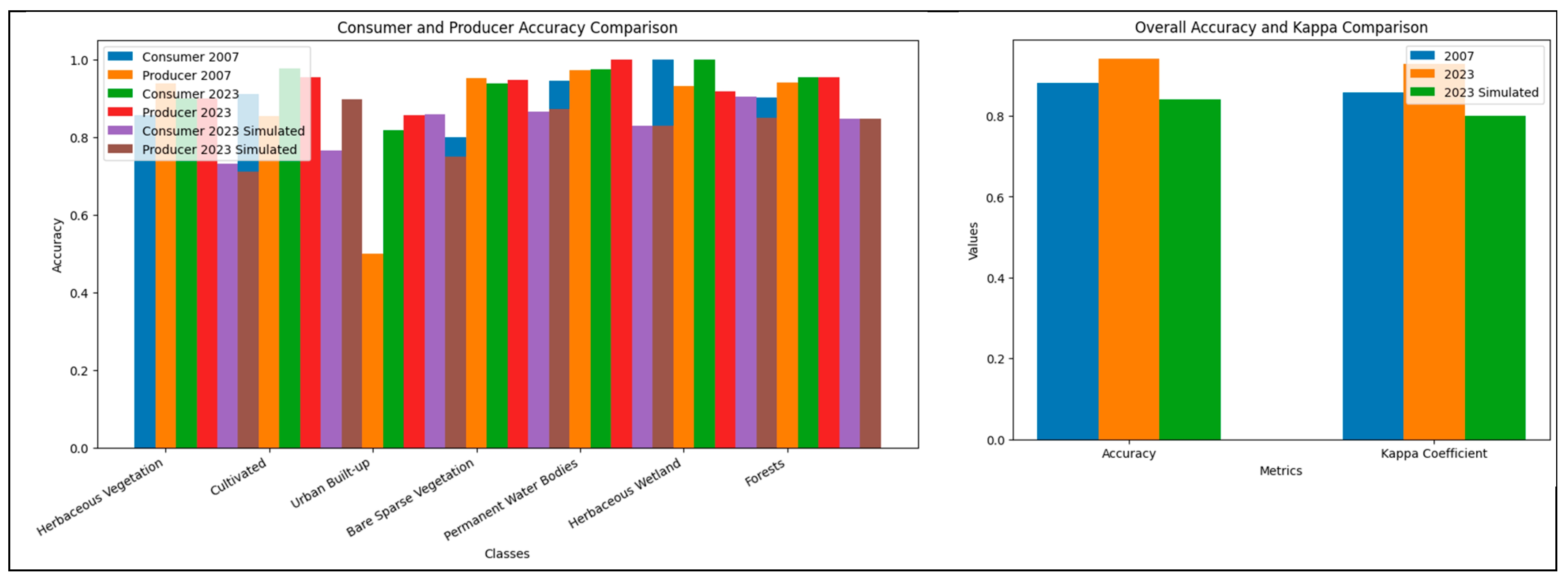
While intermediate-year data (e.g., from 2021 or 2022) could offer an additional validation step for the 2007 classification, such imagery was not incorporated into the present study. Instead, 2023 was chosen for its consistently high-quality, cloud-free observations compatible with Landsat 8 and Sentinel-1 data availability. To maintain coherence in temporal intervals, the 2019 Copernicus dataset served as a midpoint reference, refining the classification schemes and spatial distributions. Moreover, the CA–Markov modeling framework in this study employed symmetric intervals between baseline snapshots: land cover maps from 1991 and 2007 were used to simulate the 2023 distribution, then compared with the classification-derived 2023 map to evaluate model performance. Subsequently, the 2007 and 2023 land cover maps served as inputs for simulating 2040, preserving an equivalent period (16 years) to maintain consistency in transition probabilities. In addition, both the 2007 and 2023 land cover maps underwent thorough accuracy assessments with the training (30%) and testing (70%) samples, yielding overall accuracy values exceeding 88% for 2007 and 94% for 2023, as well as Kappa coefficients above 0.86 and 0.93, respectively. These metrics confirmed that the classification approach captured land cover patterns reliably in both snapshots, reducing the necessity for intermediate-year data to validate the 2007 classification.

2.4.2. Data Preprocessing and Index Computation

The initial step involved acquiring atmospherically and radiometrically corrected Landsat Level-2 imagery (Landsat 5 for 2007 and Landsat 8 for 2023) from the USGS repository in the Google Earth Engine. Additional cloud masking was applied using the QA bands to remove cloud and shadow contamination. Subsequently, several normalized difference indices were calculated to enhance the differentiation between vegetation, water, and soil/tillage features. The following indices were computed using the corresponding equations:

Normalized Difference Vegetation Index (NDVI)

NDVI leverages the contrast between near-infrared (NIR) and red reflectance to emphasize vegetation vigor. This index effectively highlights healthy vegetation characterized by a high NIR reflectance and a relatively lower red reflectance. The formulation of NDVI is expressed in Equation (8) [54]:
N D V I = N I R Re d N I R + Re d

Normalized Difference Water Index (NDWI)

Designed to enhance the identification of water bodies and moisture content, NDWI contrasts green and near-infrared reflectance. This index accentuates water pixels, exhibiting a higher green and lower NIR reflectance. Its formulation is presented in Equation (9) [55]:
N D W I = G r e e n N I R G r e e n + N I R

Normalized Difference Tillage Index (NDTI)

NDTI utilizes the contrast between two shortwave-infrared (SWIR) bands to detect soil or tillage conditions. This index highlights variations in soil brightness and agricultural residue. The formulation of NDTI is provided in Equation (10) [56]:
N D T I = S W I R 1 S W I R 2 S W I R 1 + S W I R 2
In addition to these optical indices, ancillary datasets were integrated to improve classification accuracy. NASADEM-derived elevation, slope, aspect, and landform classifications were included to capture topographic variability. Furthermore, Sentinel-1 radar backscatter data (VV, VH, and their derived combinations) were incorporated to enrich the input features, providing insights into the surface roughness and moisture, which were not discernible from optical data.

2.4.3. Classification Using Random Forest

After assembling the feature space, which included spectral bands, indices, radar data, and topographic layers, reference samples were collected for various land cover categories. These categories comprised cultivated land, herbaceous vegetation, urban areas, sparse vegetation, permanent water bodies, herbaceous wetlands, and forests. A Random Forest classifier was implemented using Google Earth Engine (GEE) scripts.
The Random Forest algorithm, an ensemble learning method, trains individual decision trees on random subsets of features and samples, introducing variability and mitigating overfitting. For each pixel, the final class assignment is determined by a majority vote across all decision trees in the ensemble [57].
The Random Forest (RF) algorithm was selected due to its robustness, interpretability, and relatively straightforward implementation within the Google Earth Engine. Unlike Support Vector Machines, which can be sensitive to parameter tuning (e.g., kernel choice, regularization parameters), RF generally requires less extensive optimization to achieve a high accuracy. Additionally, RF handles numerical and categorical variables well, is resilient to outliers, and can capture complex, non-linear relationships without overfitting as quickly as other classifiers. In this study’s multi-source remote sensing context—where features ranged from optical indices to radar backscatter—RF’s ability to leverage diverse data types and its ease of parallelization and computational efficiency made it particularly well suited for our land cover classification task [58].
Separate classification models were developed for the 2007 and 2023 datasets, resulting in two distinct land cover maps. These maps illustrate the spatial distribution of land cover classes for each period, enabling a comparative analysis of land cover changes over time.

2.4.4. Sampling Strategy for Classification and Validation

A stratified sampling approach was adopted to enhance the geospatial representativeness of the training and validation samples, ensuring that samples were not only proportional to class distributions but also spatially diverse across the study area. Given the potential for land cover heterogeneity, the sample points were systematically spread across different eco-hydrological zones to minimize spatial autocorrelation and ensure that classification models were trained on a balanced dataset reflective of real-world variability.
This sampling framework ensured that the training and validation datasets comprehensively represented the landscape, thereby improving model generalizability and enhancing the reliability of subsequent accuracy assessments.
Land cover samples were collected using the Google Earth platform, with 1097 samples selected for 2007 and 1016 for 2023. These samples were divided into two groups: 30% were designated as training samples for supervised classification, while 70% were reserved as verification points to assess classification performance.

2.4.5. Accuracy Assessment

Two standard metrics were computed to evaluate classification accuracy: Overall Accuracy (OA) and the Kappa Statistic (κ). These metrics were derived from the confusion matrix generated using the testing samples, following the standard definitions outlined below:
OA measures the proportion of correctly classified samples out of the total samples. It is calculated using the formula [59,60]:
O A = i = 1 n X i i i = 1 n j = 1 n X i j
The Kappa statistic accounts for the possibility of agreement occurring by chance. It is calculated using the following equations [61]:
P o = i = 1 n x i i N
P e = i = 1 n x i + × x + i N
K a p p a = P o P e 1 P e
where xᵢᵢ represents the Elements along the diagonal of the confusion matrix, the correct predictions for each class, and N is the total number of pixels in the dataset.
Here, Po represents the observed agreement, Pe is the expected agreement due to chance, xi+ is the sum of values in row i (total predicted for class j), and x+i is the sum of values in column i (total observed for class i).
OA provides the percentage of correctly classified samples relative to the total test samples, while k evaluates the consistency and reliability of the classification results. A higher k value signifies a stronger agreement and a greater classification accuracy, with values exceeding 0.8 typically indicating excellent performance [62].

2.5. Future Land Cover Projection in 2040

To forecast future land cover for 2040, the Cellular Automata–Markov (CA–Markov) modeling framework was employed within the TerrSet environment [63]. This methodology combines the stochastic nature of Markov Chains with the spatial explicitness of Cellular Automata (CA), providing a robust approach for simulating land cover changes over time [63].

2.5.1. Markov Chain Component

The CA–Markov model leverages the transition probability matrix to simulate prospective land use and land cover (LUCC) changes over time [64]. The Markov Chain component of the model calculates transition probabilities for land cover changes based on observed patterns from 2007 to 2023. These probabilities represent the likelihood of each land cover class transitioning into another over a defined time interval. Mathematically, the Markov process is expressed as [65]:
S t + 1 = S t × P i j
Here, S(t) is the land cover distribution vector at time t, S(t + 1) is the land cover distribution vector at time t + 1, and Pij represents the state transition probability matrix. In this matrix, each element Pij indicates the probability of transitioning from a land cover class i to j.
The transition probability matrix P is expressed as [66,67]:
P i j = P 11 P 12 ... P 1 n P 21 P 22 ... P 2 n P n 1 P n 2 ... P n n
where Pij represents the probability of transitioning from state Ei to state Ej. Constructing this matrix involves determining the transition probabilities for each state by employing the concept of frequency approximate probability, which calculates the likelihood of transitions based on historical land cover data.
The matrix P was derived from historical land cover maps, encapsulating the dynamics of land use changes over the observed period. By integrating these transition probabilities with the spatial rules of Cellular Automata, the CA–Markov model ensures a robust simulation framework that accounts for intrinsic uncertainties in land cover transitions. This powerful tool provides valuable insights for sustainable land management and long-term planning [67]. The observed transitions from 2007 to 2023 were used to calibrate the Markov transition probability matrix and the CA neighborhood rules. Calibration ensured that the model accurately captured the spatial and temporal patterns of land cover dynamics.
By integrating the temporal dynamics of Markov Chains with the spatial allocation capabilities of CA, the CA–Markov model generated a spatially explicit land cover projection for 2040. The predicted land cover map provided a plausible representation of landscape dynamics under the prevailing trends, offering a valuable baseline for subsequent climate and ecological modeling analyses [68,69].

Cellular Automata (CA) Transition Rules

In the CA–Markov framework, transition probabilities derived from historical land cover maps (2007–2023) formed the core of the Markov component. These probabilities indicated how likely a given land cover class was to transition into another over a fixed time step. The CA component then refined these transitions based on neighborhood configurations, commonly defined within a 3 × 3 or 5 × 5 window. For each cell, land cover change was influenced by the dominant transitions in its vicinity. Adjustments to adjacency rules or neighborhood size could be used to reflect distinct local processes (e.g., the tendency for wetlands to expand along river corridors). The final projected maps thus accounted for both statistical transition trends and spatial contiguity.

CA–Markov Validation

To evaluate the reliability of the CA–Markov model in simulating land cover changes, historical maps from 1991 and 2007 were used to project a 2023 scenario. The model-generated 2023 land cover was compared with the 2023 classification derived through image-based supervised methods. This comparison provided a quantitative measure of the model’s predictive accuracy, capturing how well it reflected the spatial patterns and the dominant transition processes observed over the intervening years.

2.6. MaxEnt Modeling of Wetland Presence (2023 and 2030–2050)

To model the potential presence of wetlands under current (2023) and future (2030–2050) climate conditions, we employed the Maximum Entropy (MaxEnt) modeling approach. This robust method is widely used for species and habitat distribution modeling due to its ability to effectively handle incomplete and biased presence-only data [70].

2.6.1. Variable Selection

Initially, we examined a suite of environmental and climatic variables, including minimum temperature, maximum temperature, mean temperature, annual precipitation, soil texture, slope, elevation, solar radiation, land cover, NDVI, landforms, and moisture. Correlation analysis used background data and wetland presence points to identify multicollinearity among variables. Variables showing high correlations were excluded to prevent redundancy.

2.6.2. MaxEnt Threshold Parameters

MaxEnt produces continuous habitat suitability scores ranging from 0 to 1. To convert these scores into presence/absence maps of wetlands, a threshold criterion was selected—for instance, the “maximum sensitivity plus specificity” threshold—to balance omission and commission errors. In addition, alternative thresholds (e.g., the 10th percentile training presence) could be tested for sensitivity analyses. All MaxEnt runs employed default regularization settings unless otherwise specified, ensuring reproducibility for future investigations focusing on ecological niche or habitat modeling.
This study became more transparent, repeatable, and context-rich by providing these clarifications. Future work may further enhance the analysis by incorporating in-depth socioeconomic data, applying more sophisticated speckle filters or atmospheric corrections, and conducting sensitivity tests around CA neighborhood rules and MaxEnt thresholds to explore how methodological choices influence outcomes.

2.6.3. Future Projections

For the future (2030–2050), projected climate variables under two scenarios (SSP2-4.5 and SSP5-8.5) and the 2040 land cover map were input into the Maxent model. This allowed the generation of presence probability maps for wetlands under future climatic and land use conditions. The modeling ensured consistency in the parameterization to allow direct comparisons between the current and projected periods.
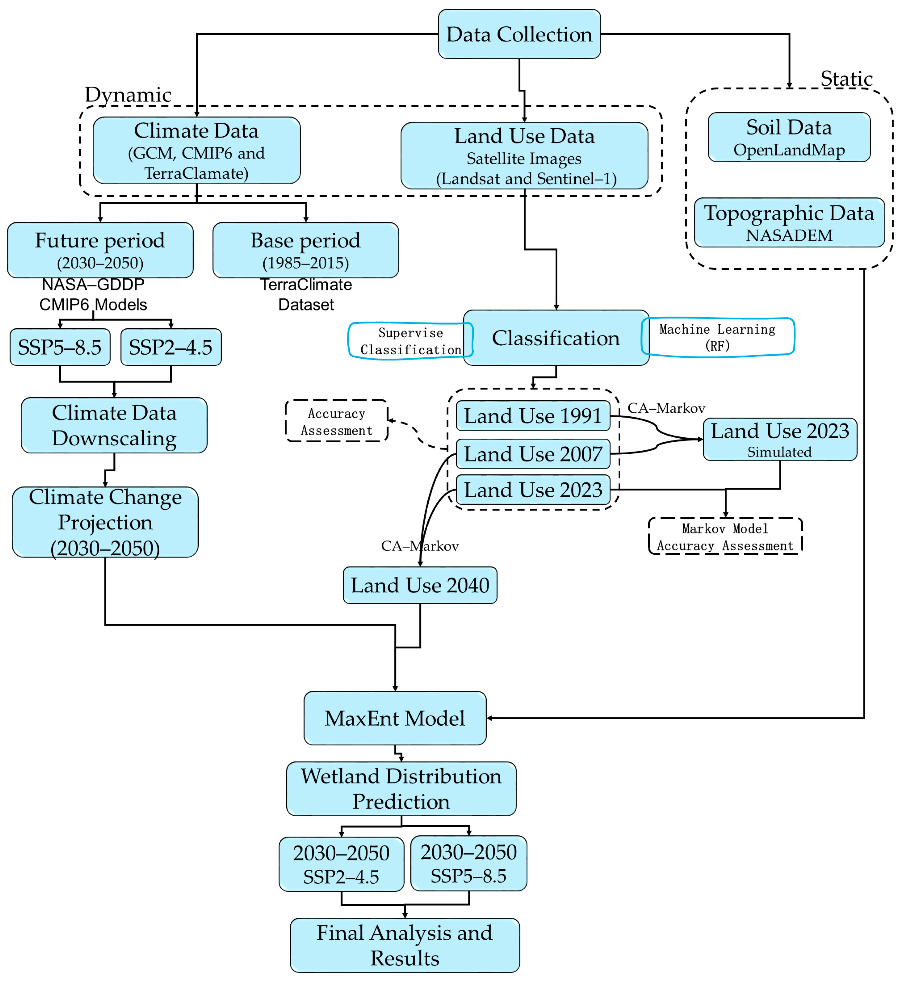
The research process is illustrated in Figure 2, providing a structured overview of the methodology employed in this study.

3. Results

3.1. Future Climate Projection and Downscaling

3.1.1. Selecting Best Model

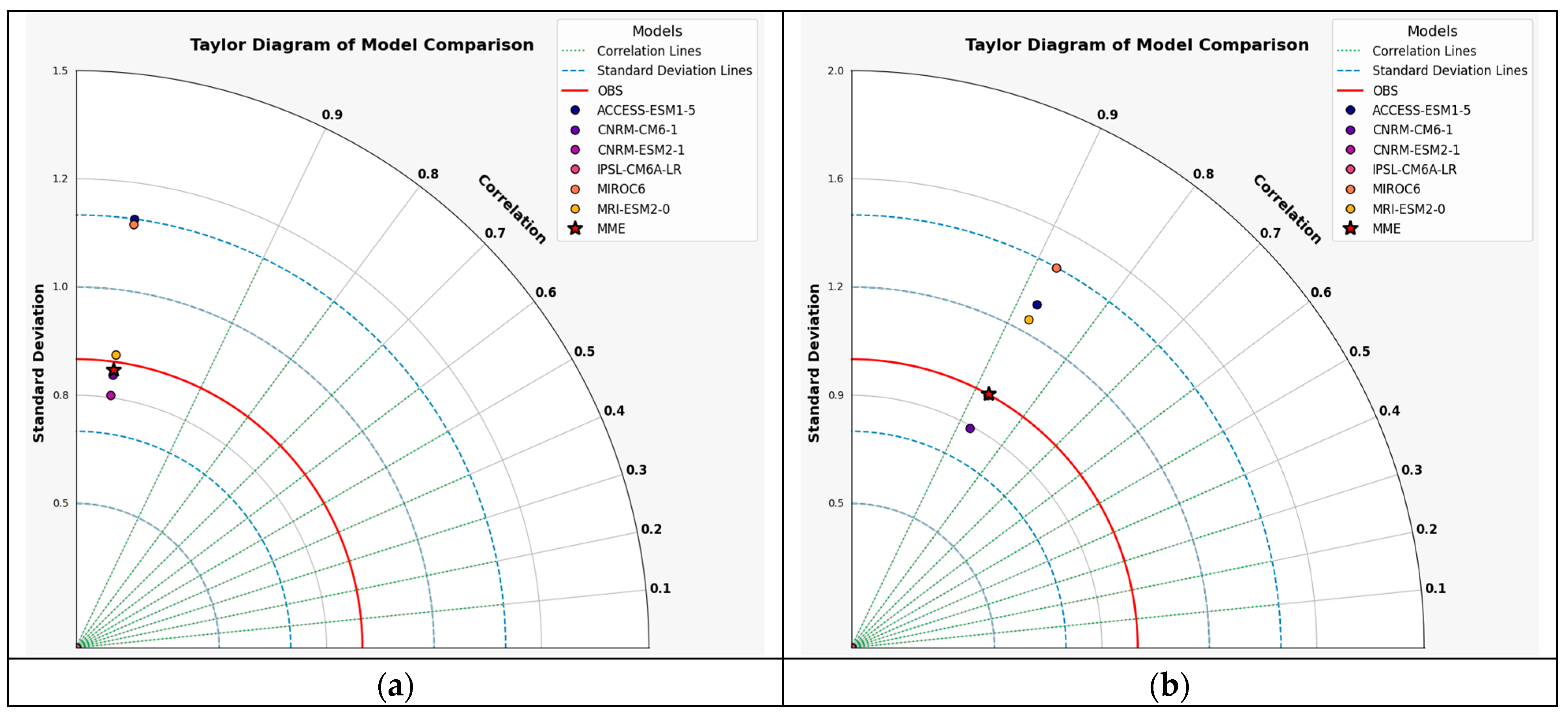
The optimal model was identified by comparing precipitation and temperature data from the historical period simulated by the models with the observed data from the baseline period (1985–2015). This comparison was conducted using correlation coefficients and standard deviations, with the data visualized through a Taylor diagram. Six individual models were evaluated alongside the ensemble model. The Taylor diagram effectively illustrated the proximity of the downscaled model’s data to the observed reference data by utilizing Pearson correlation and standard deviation. Models with smaller distances from the reference point demonstrated better alignment with the observed dataset regarding the standard deviation (SD). The performance of the models relative to each other is illustrated in Figure 3. Some model circles may not be visible as they overlap with others.
For temperature, all six individual GCMs and the multi-model ensemble (MME) exhibit highly similar performance metrics, with correlation coefficients consistently around 0.9907–0.9908. Such minimal variation in standard deviations and near-identical correlation values suggest a strong agreement between simulated temperature patterns and the observed historical dataset. The MME yields a correlation of 0.9908, indicating that the ensemble mean performs slightly better than the individual models.
In contrast, precipitation evaluation shows slightly more significant performance variability across the selected GCMs and the MME. Correlation coefficients hover around 0.8785–0.8787. Despite the relatively lower correlation compared to temperature, the consistency among models and the MME (e.g., correlation = 0.8786 for the MME) highlights the selected models’ reasonable capability to capture historical rainfall patterns.

3.1.2. Projected Temperature and Precipitation Trends (1985–2100)

Although the primary focus of this study centered on the 2030–2050 timeframe, an extended analysis from 1985 to 2100 was conducted to provide a comprehensive overview of the long-term trends and to better contextualize mid-century projections under various SSP scenarios.

Temperature Trends (1985–2100)

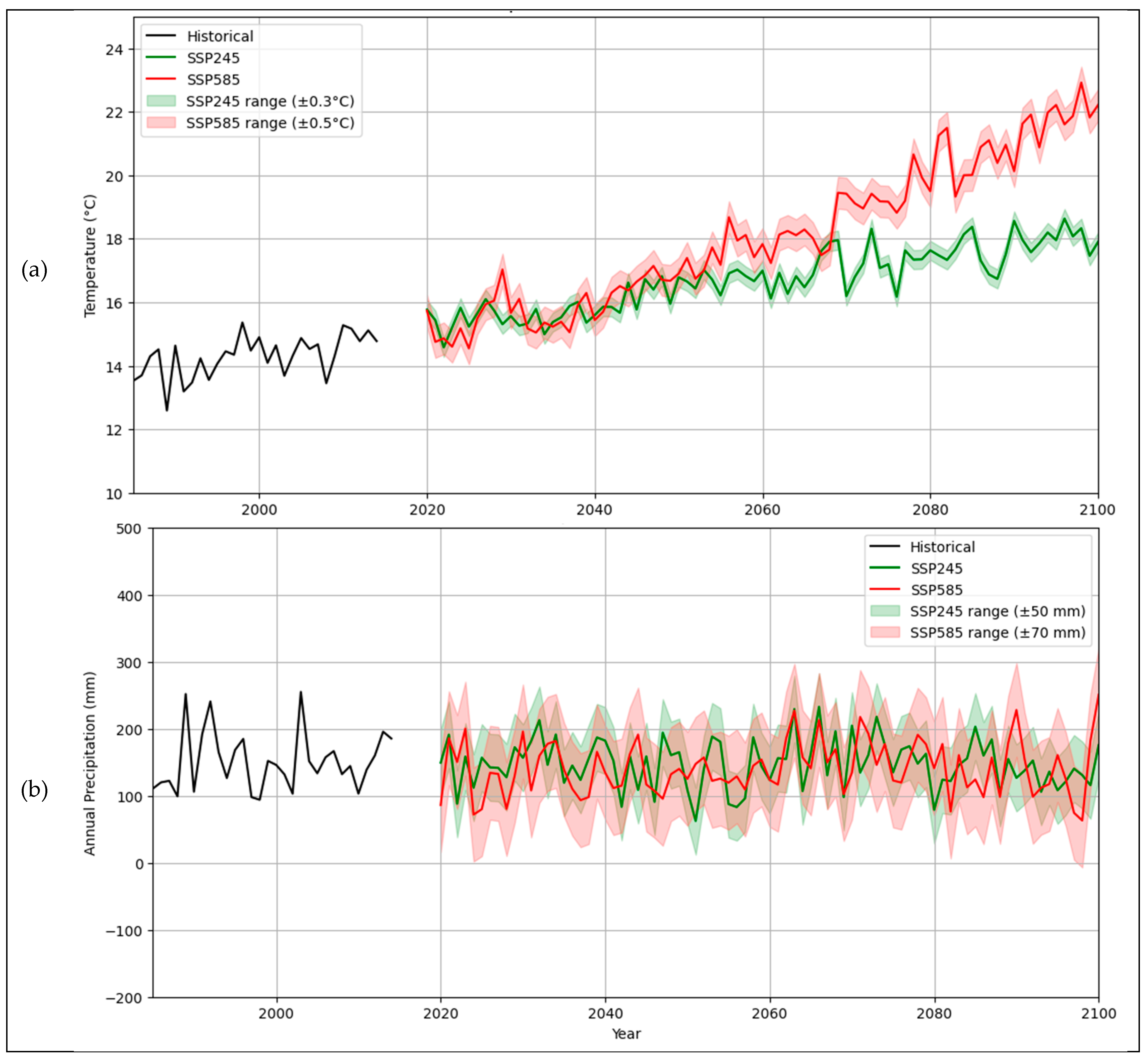
The analysis of temperature trends, as illustrated in Figure 4, reveals a marked divergence between the SSP2-4.5 and SSP5-8.5 scenarios, particularly in the latter half of the 21st century. Under the SSP245 scenario, average temperatures steadily increase, reaching approximately 22 °C by 2100, with an associated uncertainty range of ±0.3 °C. This scenario suggests a relatively moderate warming trajectory, reflecting partial mitigation efforts.
In contrast, the SSP585 scenario projects a substantially steeper temperature rise, culminating in an average temperature of approximately 24 °C by 2100 and a wider uncertainty range of ±0.5 °C. Notably, the divergence between the two scenarios becomes statistically significant around 2060, highlighting the critical impact of emission pathways on future temperature outcomes. The historical data (1985–2020) serves as a baseline, showing relatively stable trends with minor fluctuations, which are succeeded by a clear upward trajectory in both scenarios.

Precipitation Trends (1985–2100)

Figure 4 depicts the annual precipitation trends under the SSP245 and SSP585 scenarios. Both scenarios demonstrate substantial inter-annual variability, with precipitation levels oscillating within broad uncertainty ranges. Under the SSP245 scenario, the average annual precipitation stabilizes around 200 mm by the end of the century, with a range of ±50 mm. This suggests a relatively consistent precipitation pattern, albeit with occasional deviations.
Under the SSP585 scenario, precipitation exhibits greater variability and a marginal upward trend, reaching an average of approximately 220 mm by 2100, with a broader uncertainty range of ±70 mm. The overlapping uncertainty bands between the two scenarios throughout the 21st century indicate potential challenges in distinguishing the effects of different emission pathways on precipitation patterns. Nonetheless, the SSP585 scenario suggests a higher likelihood of extreme precipitation events due to the amplified variability.
The considerable spread among precipitation projections shown in Figure 4 primarily reflects the inherent difficulties in modeling regional rainfall patterns. Unlike temperature, which is often more uniformly simulated, precipitation exhibits a higher variability because it responds to various local atmospheric processes and terrain influences. Each General Circulation Model (GCM) employs distinct physical parameterizations and boundary conditions, resulting in divergent precipitation outputs even under the same emission scenario. This study presents the multi-model mean alongside the uncertainty ranges (e.g., ±50 mm under SSP2-4.5 and ±70 mm under SSP5-8.5) to capture this variability. Such an approach follows recognized practices in climate impact assessments and provides stakeholders with a more realistic window of future conditions. By recognizing these uncertainties, decision-makers can develop more robust adaptation and mitigation strategies, acknowledging that any single model may not fully capture the breadth of possible outcomes.

Sub-Region-Level Precipitation Changes (2030–2050)

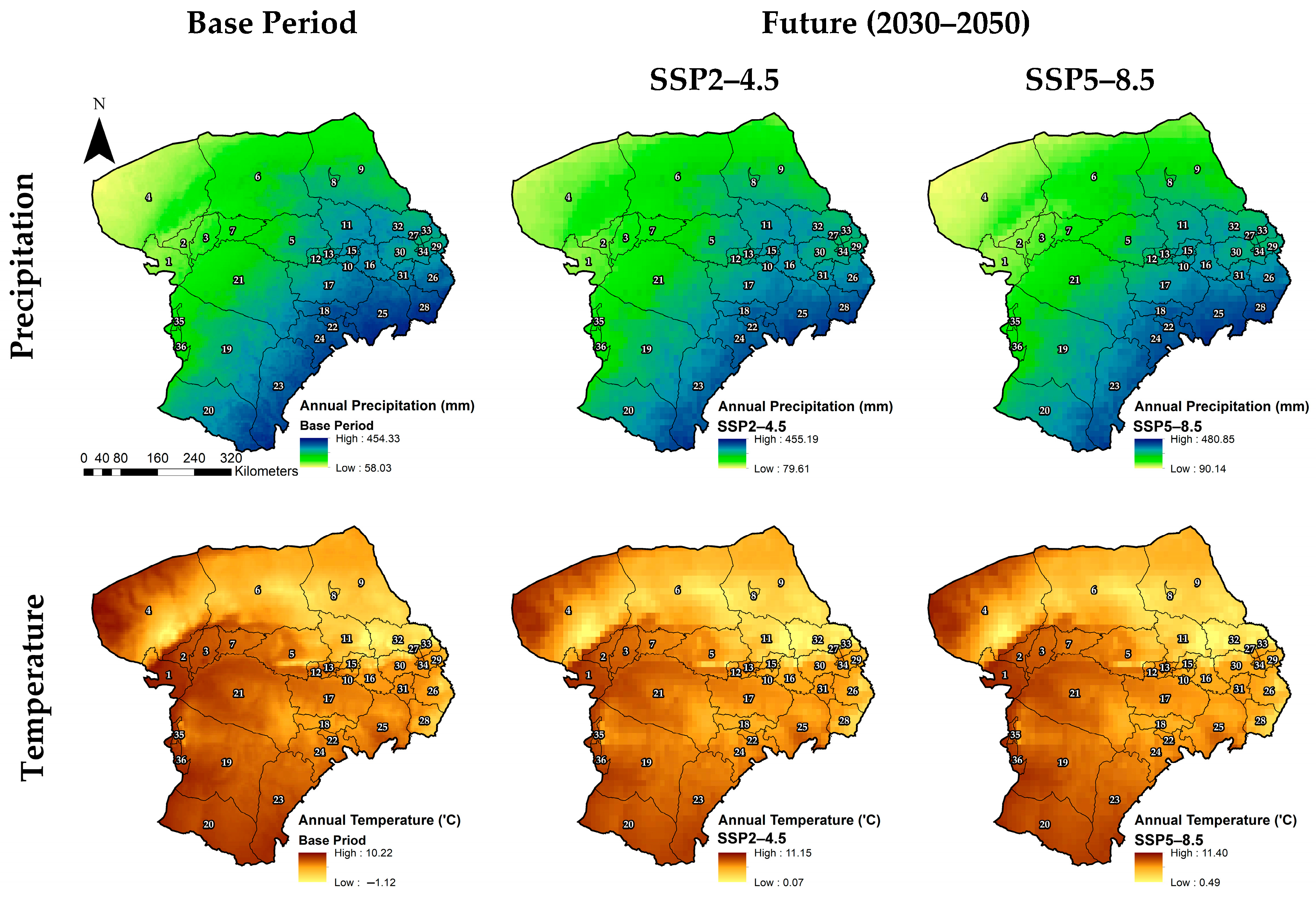
An examination of the baseline and projected precipitation values (2030–2050) under different climate scenarios (SSP2-4.5 and SSP5-8.5) demonstrates a consistent upward trend across most sub-regions (Figure 5). For instance, Linhe District shows a current precipitation of 142.27 mm, increasing to 163.33 mm under SSP2-4.5 and 162.51 mm under SSP5-8.5. A similar pattern emerges in Hanging Banner, where precipitation is projected to rise from 227.28 mm to 235.21 mm (SSP2-4.5) and 253.21 mm (SSP5-8.5). These findings suggest that many areas in the study region may experience moderate-to-substantial increases in precipitation over the coming decades.
Certain sub-regions exhibit particularly pronounced changes. For example, Qingshuihe County displays a baseline precipitation of 387.99 mm, rising to 385.33 mm under SSP2-4.5 and 414.54 mm under SSP5-8.5—indicating one of the most considerable scenario-based differences in the dataset. Likewise, Jungar Banner’s precipitation is expected to increase from 379.93 mm in the baseline period to 376.28 mm (SSP2-4.5) and 405.78 mm (SSP5-8.5), highlighting a marked rise under the high-emission scenario. Kangbashi District also shows a notable increase, transitioning from 362.37 mm to 358.93 mm (SSP2-4.5) and further to 390.82 mm (SSP5-8.5), suggesting heightened precipitation extremes in that locality.
By contrast, a few sub-regions, though still exhibiting growth, display more moderate changes. Wuyuan County, for instance, is projected to rise from 169.19 mm to 187.11 mm (SSP2-4.5) and 184.45 mm (SSP5-8.5). Urat Middle Banner shows an initial precipitation of 184.70 mm, expected to climb to 200.75 mm under SSP2-4.5 and 191.77 mm under SSP5-8.5, indicating a modest albeit consistent increase. Taken together, these results underscore a region-wide intensification of precipitation regimes shortly, with certain sub-regions likely to experience particularly robust gains in annual rainfall under higher emission scenarios (Figure 5).

Sub-Basin-Level Temperature Changes (2030–2050)

An examination of the baseline and projected temperature values (2030–2050) under different climate scenarios (SSP2-4.5 and SSP5-8.5) reveals a clear warming trend across the study area (Figure 5). For instance, Wuchuan County, which currently exhibits one of the lowest baseline temperatures (3.69 °C), is projected to increase to 4.71 °C under SSP2-4.5 and 4.69 °C under SSP5-8.5. Conversely, Wuda District displays among the highest baseline temperatures (9.08 °C), rising to 9.93 °C (SSP2-4.5) and 10.37 °C (SSP5-8.5). This notable contrast highlights the heterogeneity of thermal conditions within the region.
Several sub-regions demonstrate substantial increases under the high-emissions scenario (SSP5-8.5). Hainan District, for example, shows an upward shift from a current mean of 8.80 °C to 9.66 °C under SSP2-4.5 and 10.11 °C under SSP5-8.5—representing one of the largest overall changes in the dataset. A similarly pronounced pattern is observed in Uxin Banner, which moves from 8.14 °C at baseline to 9.07 °C (SSP2-4.5) and 9.29 °C (SSP5-8.5). In comparison, sub-regions such as Tumed Left Banner exhibit more moderate shifts, increasing from 5.97 °C to 7.03 °C (SSP2-4.5) and 6.98 °C (SSP5-8.5).
Notably, certain areas start with relatively cooler baseline temperatures yet still display robust warming trends. Baiyun Ebo Mining District, for instance, is projected to rise from 4.43 °C to around 5.39–5.42 °C under both future scenarios, while Shiguai District’s temperature climbs from 5.17 °C to approximately 6.22–6.26 °C. Overall, these results underscore a consistent regional temperature increase in the coming decades, with the SSP5-8.5 scenario generally inducing greater warming than SSP2-4.5. Such findings reinforce the importance of incorporating targeted climate adaptation strategies across diverse sub-regions within the study domain (Figure 5).

3.2. Land Cover Classes in the Study Area

A detailed assessment of the CGLS-LC100 product for the study area revealed the land cover categories summarized in Table 3. These classes served as the foundation for further land cover analysis and classification.

3.3. Land Cover Mapping for 2007 and 2023

Between 2007 and 2023, the study area experienced notable shifts across multiple land use categories (Figure 6). Herbaceous vegetation exhibited a slight increase from approximately 12.10 million ha to 12.14 million ha, while cultivated lands grew from 3.21 million ha to 3.41 million ha, suggesting a moderate agricultural expansion. Urban built-up areas rose particularly sharply, climbing from about 39.53 thousand ha to 218.88 thousand ha. Bare sparse vegetation decreased from 10.25 million ha to 9.94 million ha, pointing to ongoing land conversion processes. Notably, permanent water bodies almost doubled from approximately 89.07 thousand ha to 155.19 thousand ha, whereas herbaceous wetlands experienced a dramatic reduction, shrinking from 100.59 thousand ha to only 5.18 thousand ha. Forest cover also declined, dropping from 439.39 thousand ha to 357.38 thousand ha, indicating pressures on wetland and forested ecosystems.

Accuracy Assessment

Figure 6 presents the overall accuracy and Kappa coefficients for 2007 and 2023. Both metrics indicate a high classification performance in both years. The overall accuracy was 0.88 in 2007 and 0.94 in 2023, while the Kappa coefficient reached 0.86 and 0.93, respectively. These values highlight the classification methodologies’ robustness and the data processing reliability across both periods. The CA–Markov model was also evaluated by comparing its simulated 2023 map with the actual 2023 classification. This assessment yielded an overall accuracy of 0.83 and a Kappa coefficient 0.79, indicating a strong alignment between the model projections and the observed land cover. These updated accuracy metrics suggest an improved reliability of the model in capturing land cover transitions and spatial dynamics within the study area. Moreover, they are consistent with the findings reported in [67,71,72,73,74,75], where CA–Markov approaches likewise demonstrated high classification accuracy and robust predictive capabilities for land cover simulations in comparable settings.

3.4. Future Land Cover Projection in 2040

Projections for 2040 suggest the continuation of several existing trends, with herbaceous vegetation further increasing from 12.14 million ha to 12.72 million ha and cultivated lands expanding from 3.41 million ha to 3.56 million ha (Figure 7). Urban built-up areas are expected to rise more modestly, from 218.88 thousand ha to 251.00 thousand ha, yet still reflecting ongoing urbanization. Bare sparse vegetation is projected to decline further, decreasing from 9.94 million ha to 9.24 million ha. Permanent water bodies will see a minor gain, moving from 155.19 thousand ha to 161.73 thousand ha, whereas herbaceous wetlands will show a slight reduction, from 5.18 thousand ha to 5.00 thousand ha. A significant concern is the sharp decline in forest cover, projected to drop from 357.38 thousand ha to 173.08 thousand ha, underscoring the continued vulnerability of woody ecosystems and the critical need for targeted conservation measures (Figure 7).

3.5. Analysis of Land Cover Transition and Change

3.5.1. Change Analysis Between 2007 and 2023

Figure 8 presents three zoomed-in areas (labeled a, b, and c) that illustrate the localized wetland dynamics within the study region for 2007, 2023, and 2040. These panels highlight the spatial distribution of multiple land use/land cover classes (e.g., herbaceous vegetation, cultivated lands, bare/sparse vegetation, permanent water bodies, and herbaceous wetlands), enabling a closer examination of how wetland patches evolve in representative case studies.
In area (a), herbaceous wetlands and permanent water bodies along the river corridor are gradually converted to cultivated lands. Between 2007 and 2023, there is a marked reduction in wetlands, coinciding with an expansion of croplands. Projections for 2040 further suggest the continued encroachment of cultivated areas, underscoring the vulnerability of riparian wetlands to agricultural intensification.
Area (b) shows a similar trend, transitioning from wetlands to cultivated lands and urban/built-up areas. While some permanent water bodies persist, the overall extent of the wetland diminishes markedly from 2007 to 2040, parallel with the growing urban development (black) in the surrounding landscapes.
In area (c), the wetland zone flanking the main river system likewise undergoes conversion. Wetlands initially prominent in 2007 are gradually replaced by herbaceous vegetation and croplands. Although portions of the permanent water bodies remain, the overall pattern signals a net loss of herbaceous wetlands by 2040.

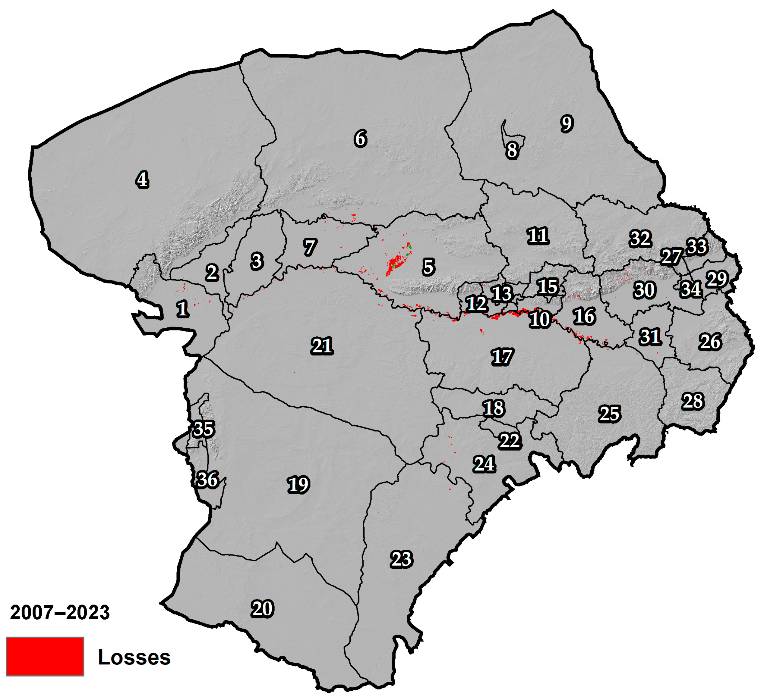
3.5.2. Gains and Losses Between 2007 and 2023

Figure 9a illustrates the gains and losses across various land cover types between 2007 and 2023. The most significant changes are observed in the herbaceous vegetation and cultivated areas, which experienced substantial gains, exceeding 200,000 hectares each. Conversely, bare, sparse vegetation showed significant losses, surpassing 200,000 hectares, indicating notable transitions between land cover types. Urban built-up areas also displayed moderate gains, reflecting increased anthropogenic activity, while smaller scale changes occurred in forests, herbaceous wetlands, and permanent water bodies. These results highlight the dynamic nature of land cover changes over the study period.
Figure 9b presents the net changes in land cover types from 2007 to 2023. Herbaceous vegetation exhibited the highest net increase, surpassing 300,000 hectares, followed by cultivated and urban built-up areas, which also recorded positive net changes. In contrast, bare sparse vegetation experienced the most substantial net decrease, followed by forests and herbaceous wetlands, with declines of approximately 200,000 hectares and 100,000 hectares, respectively. These net changes underline the significant transformation of land cover types, driven by natural and anthropogenic factors.
Figure 9c analyzes the contributions of various land cover types to the net change in herbaceous wetlands. The most prominent contributor to the decline in herbaceous wetlands was the conversion to cultivated land, which accounted for most of the observed decrease. Additionally, herbaceous vegetation and urban built-up areas contributed to this reduction, albeit to a lesser extent. Minor contributions to the decline were also noted from bare sparse vegetation. These findings emphasize the critical impact of land use changes on herbaceous wetland ecosystems.

3.5.3. Gains and Losses Between 2023 and 2040

The comparative bar charts (Figure 10a) illustrate the gains and losses in different land use categories between 2023 and 2040, along with the net changes and the specific contributions driving the shifts in herbaceous wetlands. The most substantial net gain is evident in herbaceous vegetation, followed by more moderate increases in cultivated land and urban built-up areas. In contrast, bare sparse vegetation and forests experience the largest net losses, suggesting continued pressures on woody ecosystems and sparsely vegetated landscapes (Figure 10a).
In particular, the first chart (gains and losses between 2023 and 2040) reveals that herbaceous vegetation shows the greatest positive change, whereas forests and bare sparse vegetation register pronounced declines. Urban built-up and cultivated areas increase modestly, reflecting ongoing agricultural expansion and urbanization. The second chart (net change between 2023 and 2040) confirms these overall trajectories, emphasizing the net expansion in herbaceous vegetation—surpassing 600,000 m2—and a significant contraction in forests (over 300,000 m2 lost). This highlights the extent of habitat conversion, potentially driven by anthropogenic and climatic factors (Figure 10b).
The third chart (contributions to net change in herbaceous wetland) underscores how multiple land use categories influence changes in herbaceous wetlands. Forests and bare sparse vegetation appear to be the primary sources of wetland conversion, while cultivated land and urban areas also contribute to the overall net loss. Although herbaceous wetland decline is less extensive than other categories, the data suggest that continuous encroachment and land use transformation remain key concerns for wetland sustainability. These findings point to ongoing regional land use reconfigurations, emphasizing the need for targeted management strategies to balance ecological integrity with developmental objectives (Figure 10c and Figure 11).

3.6. MaxEnt Modeling of Wetland Presence (2023 and 2030–2050)

3.6.1. Correlation Analysis of Environmental Variables

Table 4 presents the correlations among the environmental variables. Significant relationships are observed between several variables in Table 4, representing background correlations. For example, precipitation and humidity showed a strong positive correlation (r = 0.90), while temperature variables (mean, maximum, and minimum temperature) exhibited near-perfect correlations (r > 0.99), indicating potential redundancy. Elevation demonstrated moderate negative correlations with temperature variables (r ≈ −0.52), reflecting its indirect influence on climatic conditions.
To ensure the MaxEnt model’s robustness and interpretability, variables with high inter-correlations were excluded from further analysis. For instance, mean temperature was retained among the temperature metrics due to its representative nature, while maximum and minimum temperatures were excluded to avoid redundancy. Similarly, closely related variables such as precipitation and humidity were carefully evaluated to retain only the most relevant predictors (Figure 12).
This process of variable selection ensured that the final set of predictors was both independent and representative, minimizing the risk of multicollinearity while enhancing the model’s predictive performance.

3.6.2. Model Performance and Variable Importance in MaxEnt

The Jackknife test highlights temperature, precipitation, and land use as the most influential predictors for wetland occurrence, as each produces a high AUC when tested independently. The emission curve demonstrates low divergence between the predicted area and the observed omission rates, reflecting its overall robustness across various threshold values. Finally, the ROC curve achieves an AUC of 0.983, underscoring the high predictive power of the MaxEnt model in distinguishing wetland presence from absence. These findings collectively indicate that the model is accurate and reliable, with a few key environmental variables (notably temperature and precipitation) exerting dominant roles in determining wetland habitat suitability.

3.6.3. MaxEnt Modeling Results: Present and Future Wetland Suitability Across Administrative Subdivisions

The MaxEnt model outputs indicate varying probabilities of wetland presence across the 40 administrative sub-regions under current and future climate scenarios (Figure 1). Under present conditions, Haibowan District exhibits the highest probability of wetland presence (average = 0.2436), followed by Hainan District (0.0435) and Wuda District (0.0595). In contrast, Baiyun Ebo Mining District shows the lowest probability (3.99 × 10⁻⁵). Moving to the SSP2-4.5 scenario, most subdivisions experience a noticeable decline. For instance, the Urat Front Banner drops from 0.0454 to 0.0339, and Haibowan District decreases from 0.2436 to 0.1643. Exceptions include Shiguai District, which slightly increases from 0.00378 to 0.00387 (Figure 13).
Under the more extreme SSP5-8.5 scenario, this declining trend continues in many areas. Haibowan District falls further to 0.1513, and Wuda District decreases from 0.0595 to 0.0458. Nonetheless, a few locations, such as Shiguai District (increasing to 0.00414) and Wuchuan County (rising from 0.00167 to 0.00212), display marginal gains. These results suggest that future climate scenarios will likely reduce the wetland presence across the region, although the magnitude and direction of these changes will vary by subdivision. This spatial heterogeneity underscores the need for targeted conservation and management strategies, as certain districts may be more vulnerable to future climate shifts. In contrast, others could retain or slightly increase their wetland habitat suitability (Figure 13).

4. Discussion

The present study underscores the intricate interplay between climate change, land use dynamics, and wetland suitability in the Yellow River Watershed. By integrating advanced climate projections (NASA’s GDDP and IPCC AR6), CA–Markov simulations of land use transitions, and MaxEnt habitat suitability modeling, our findings converge on a critical insight: wetland ecosystems in this semi-arid region are under mounting pressure from both intensifying climatic stressors and rapid anthropogenic modifications. This section provides a holistic discussion of how these factors intersect, drawing comparisons with analogous research and articulating regional conservation and management implications.

4.1. Climate Change and Wetland Hydrology

Projections under moderate (SSP2-4.5) and high-emission (SSP5-8.5) pathways show warming trends consistent with IPCC (2021) and related large-scale studies [76], indicating that higher temperatures will increase evapotranspiration rates and potentially exacerbate water deficits in local wetlands. Although some sub-basins in our study (e.g., Qingshuihe County) are expected to receive slightly more annual precipitation, the anticipated shifts toward more erratic rainfall patterns raise concerns regarding the stability of wetland hydrological regimes. Such temporal variability—with occasional floods interspersed by prolonged dry spells—has also been documented in other semi-arid zones of northern China [77] and globally [78]. These studies consistently note that increases in precipitation are often counteracted by intensified evapotranspiration and land surface changes, underscoring that any net benefit of higher rainfall may be undermined by ongoing warming and greater vapor loss. Consequently, the overall trajectory points to a contraction of wetland areas, particularly herbaceous wetlands, and an increased susceptibility to hydrological extremes.

4.2. Land Use Transitions and Ecological Consequences

The CA–Markov analysis confirms that rapid agricultural expansion and urbanization remain key drivers of wetland loss—mirroring broader patterns of ecosystem transformation reported in other parts of China [79] and globally [80]. Our results reveal both “stable” land cover classes (e.g., large tracts of herbaceous vegetation and persistent water bodies) and areas undergoing significant shifts, especially in converting herbaceous wetlands to cropland and urban/built-up zones. This pattern resonates with [81] and [79], who emphasize how agriculture-driven land use changes can drastically reduce natural habitats and modify local microclimates, leading to cascading ecological effects such as biodiversity loss and soil degradation.
Another noteworthy transition is the conversion of “Permanent Water Bodies” to “Herbaceous Wetlands”, potentially reflecting sedimentation, nutrient loading, or declining water tables that encourage emergent vegetation. While this process can locally enhance habitat heterogeneity—offering niche conditions for certain wetland species—it may also reduce open-water habitats essential for waterfowl or fish [82]. Similarly, instances of “Bare Sparse Vegetation” transitioning to “Permanent Water Bodies” may arise from anthropogenic reservoir construction or extreme climate events, yielding outcomes that hinge on the surrounding socio-environmental context. These findings align with prior regional assessments [83] that highlight the multifaceted nature of land cover dynamics, wherein the same process (e.g., creation of water bodies) can prove beneficial for wetland species in some locations but detrimental elsewhere, by displacing farmland or terrestrial habitats.
Of particular concern is the simultaneous decline of forests alongside wetlands. Both ecosystems play fundamental roles in carbon sequestration, local climate regulation, and biodiversity conservation, and their dual degradation suggests a deeper trend of ecological stress in the region. Studies in other parts of northern China have recorded similar “co-decline” scenarios [84], often attributable to concurrent logging pressures, agricultural intensification, and urban expansion. This convergence of stressors underscores the urgency of integrated land use policies encompassing forests, wetlands, and agricultural zones rather than managing each land cover type in isolation.
Although this study primarily focuses on climate- and land-use-driven changes, socioeconomic factors also play a crucial role in shaping wetland dynamics. In semi-arid regions, irrigation intensity, dam and reservoir construction, and agricultural management policies can substantially alter hydrological regimes. For instance, heightened irrigation intensity can reduce water availability downstream. At the same time, dam and reservoir operations can stabilize or drastically modify flow patterns depending on seasonal water storage and release schedules. Similarly, agricultural subsidies or land use regulations may incentivize converting marginal wetlands into croplands or may encourage their preservation. Collectively, these factors form an intricate network of human–environment interactions that merits further exploration, especially in long-term wetland conservation frameworks.

4.3. MaxEnt Modeling and Spatial Heterogeneity

The MaxEnt results indicate that temperature, precipitation, and land use characteristics are pivotal to wetland suitability. High AUC values (exceeding 0.98) confirm the robust performance of this modeling approach, aligning with the conclusions of [85] and [86] regarding the suitability of MaxEnt for capturing complex non-linear habitat relationships. While the overall trend points to future declines in wetland suitability—particularly under the SSP5-8.5 pathway—our analysis reveals spatial heterogeneity. Districts such as Haibowan and Urat Front Banner, currently rich in wetland habitats, are projected to experience a significant deterioration of suitability if warming and land use intensification continue unabated. In contrast, Shiguai District may see minor improvements, suggesting that localized factors (e.g., topography, hydrogeology, or shifts in cropping patterns) can partially offset broader climatic stressors.
These nuances underscore the need for region-specific strategies. Local governance and resource management practices, including water allocation policies and conservation incentives, may ultimately determine whether a given sub-region can maintain some ecological resilience. Similar conclusions arise in international case studies of wetland conservation [87], demonstrating that while macro-scale climate forces set the overarching context, micro-scale interventions can shape the on-the-ground realities.

4.4. Implications for Conservation and Policy

The converging evidence of the warming climate, variation in precipitation, and aggressive land use expansion underscores an urgent need for integrated, science-based conservation policies. First, wetland protection laws should be strengthened to limit further encroachment by agriculture and urban development, particularly in ecologically sensitive districts. Second, adaptive land use planning—coordinated at multiple administrative levels—must address both hydrological extremes and incremental wetland loss, for instance, by incentivizing water-efficient cropping systems and enforcing zoning regulations in flood-prone or high-biodiversity zones. Third, restoration programs designed to re-establish degraded wetlands and forests can offer co-benefits for carbon storage, flood mitigation, and biodiversity. Such approaches are widely recommended in the literature [88], although their successful implementation depends on financing mechanisms, local stakeholder engagement, and long-term ecological monitoring.
Furthermore, the spatially explicit nature of MaxEnt outputs can inform the prioritization of conservation efforts, directing resources to high-probability wetland zones which are at the most significant risk under future scenarios. This approach aligns with recent practices in conservation planning, where fine-scale habitat suitability maps guide the allocation of management interventions [89]. Lastly, cross-sectoral collaboration is essential: aligning the interests of agriculture, urban development, and environmental agencies can foster policies that balance economic growth with ecological sustainability. Without such synergy, the continued decline of both wetlands and forests remains a likely outcome, compromising critical ecosystem services for future generations.

5. Conclusions

Overall, the findings of this study portray a region on the cusp of transformative change, with wetland ecosystems facing intersecting pressures from intensifying climate stressors and expanding land use demands. Although certain localities might experience transient gains or relatively stable wetland cover, the dominant trend is a gradual decline in habitat suitability, especially under high-emission scenarios. Comparisons with parallel research in northern China and worldwide confirm that these forces are far from unique; instead, they form part of a broader pattern of wetland vulnerability to global climatic shifts and localized land use transitions. Given the ecological importance of wetlands in regulating water flow, maintaining biodiversity, and supporting livelihoods, an integrated and adaptive management framework—backed by robust policy commitments—will be crucial for sustaining these fragile ecosystems in the decades ahead.

Author Contributions

Conceptualization, P.J. and R.S.; methodology, P.J.; software, R.S.; validation, P.J. and R.S.; formal analysis, P.J.; investigation, R.S.; resources, P.J.; data curation, P.J.; writing—original draft preparation, P.J. and R.S.; writing—review and editing, P.J., R.S., G.W., L.X., Z.Z., H.F., R.G., W.Z. and D.Z.; visualization, L.X.; supervision, R.G.; project administration, R.G.; funding acquisition, P.J. and H.F. All authors have read and agreed to the published version of the manuscript.

Funding

This research was jointly funded by National Natural Science Foundation of China (Grant No. 32360249), the Key research and development and results transformation plan (Grant No. 2023YFDZ0017), the Inner Mongolia Agricultural University young teachers research ability promotion project (Grant No. BR230161), the Baotou Wetland Resources Survey and Monitoring Project (Grant No. RH2200001332), Physical Inventory of Wetland Resource Assets in Hohhot and Ordos (Grant No. RH2400000841), and the University Scientific Research Project of Inner Mongolia Autonomous Region of China (No. NJZY22484).

Data Availability Statement

The data presented in this study are available on request from the corresponding author.

Conflicts of Interest

The authors declare no conflicts of interest.

References

  1. Mitsch, W.J.; Bernal, B.; Hernandez, M.E. Ecosystem Services of Wetlands. Int. J. Biodivers. Sci. Ecosyst. Serv. Manag. 2015, 11, 1–4. [Google Scholar] [CrossRef]
  2. Zedler, J.B.; Kercher, S. Wetland Resources: Status, Trends, Ecosystem Services, and Restorability. Annu. Rev. Environ. Resour. 2005, 30, 39–74. [Google Scholar] [CrossRef]
  3. Ge, G.; Zhang, J.; Chen, X.; Liu, X.; Hao, Y.; Yang, X.; Kwon, S. Effects of Land Use and Land Cover Change on Ecosystem Services in an Arid Desert-Oasis Ecotone along the Yellow River of China. Ecol. Eng. 2022, 176, 106512. [Google Scholar] [CrossRef]
  4. Dale, V.H.; Brown, S.; Haeuber, R.A.; Hobbs, N.T.; Huntly, N.; Naiman, R.J.; Riebsame, W.E.; Turner, M.G.; Valone, T.J. Ecological Principles and Guidelines for Managing the Use of Land Sup> 1. Ecol. Appl. 2000, 10, 639–670. [Google Scholar]
  5. Erwin, K.L. Wetlands and Global Climate Change: The Role of Wetland Restoration in a Changing World. Wetl. Ecol. Manag. 2009, 17, 71–84. [Google Scholar] [CrossRef]
  6. Grimm, N.B.; Chapin, F.S., III; Bierwagen, B.; Gonzalez, P.; Groffman, P.M.; Luo, Y.; Melton, F.; Nadelhoffer, K.; Pairis, A.; Raymond, P.A. The Impacts of Climate Change on Ecosystem Structure and Function. Front. Ecol. Environ. 2013, 11, 474–482. [Google Scholar] [CrossRef]
  7. Sarkar, D.; Maji, N. Status and Threats of Wetland Change in Land Use Pattern and Planning: Impact of Land Use Patterns and Urbanization. In Handbook of Research on Monitoring and Evaluating the Ecological Health of Wetlands; IGI Global: Hershey, PA, USA, 2022; pp. 106–127. [Google Scholar]
  8. Gavrilescu, M. Water, Soil, and Plants Interactions in a Threatened Environment. Water 2021, 13, 2746. [Google Scholar] [CrossRef]
  9. Admas, M.; Melesse, A.M.; Tegegne, G. Predicting the Impacts of Land Use/Cover and Climate Changes on Water and Sediment Flows in the Megech Watershed, Upper Blue Nile Basin. Remote Sens. 2024, 16, 2385. [Google Scholar] [CrossRef]
  10. Zhou, F.; Dong, X.; Li, J.; Zhou, W.; Zhao, C.; Gang, C. Quantitative Assessment of the Individual Contribution of Climate and Human Factors to Desertification in Northwest China Using Net Primary Productivity as an Indicator. Ecol. Indic. 2014, 48, 560–569. [Google Scholar] [CrossRef]
  11. Kong, X.; Han, M.; Li, Y.; Kong, F.; Sun, J.; Zhu, W.; Wei, F. Spatial Differentiation and Formation Mechanism of Ecological Sensitivity in Large River Basins: A Case Study of the Yellow River Basin, China. Ecol. Indic. 2024, 158, 111571. [Google Scholar] [CrossRef]
  12. Mukonza, S.S.; Chiang, J.-L. Meta-Analysis of Satellite Observations for United Nations Sustainable Development Goals: Exploring the Potential of Machine Learning for Water Quality Monitoring. Environments 2023, 10, 170. [Google Scholar] [CrossRef]
  13. Mohanty, S.; Pandey, P.C.; Srivastava, P.K.; Srivastava, S.K. Challenges and Future Implications in Monitoring and Assessment of Aquatic Ecosystems. In Aquatic Ecosystems Monitoring; CRC Press: Boca Raton, FL, USA, 2025; pp. 297–318. [Google Scholar]
  14. Ozesmi, S.L.; Bauer, M.E. Satellite Remote Sensing of Wetlands. Wetl. Ecol. Manag. 2002, 10, 381–402. [Google Scholar] [CrossRef]
  15. Guo, M.; Li, J.; Sheng, C.; Xu, J.; Wu, L. A Review of Wetland Remote Sensing. Sensors 2017, 17, 777. [Google Scholar] [CrossRef]
  16. Rawat, K.S.; Kumar, S.; Garg, N. Statistical Comparison of Simple and Machine Learning Based Land Use and Land Cover Classification Algorithms: A Case Study. J. Water Manag. Model. 2024, 32, H524. [Google Scholar] [CrossRef]
  17. Wang, J.; Bretz, M.; Dewan, M.A.A.; Delavar, M.A. Machine Learning in Modelling Land-Use and Land Cover-Change (LULCC): Current Status, Challenges and Prospects. Sci. Total Environ. 2022, 822, 153559. [Google Scholar] [CrossRef]
  18. Abatzoglou, J.T.; Dobrowski, S.Z.; Parks, S.A.; Hegewisch, K.C. TerraClimate, a High-Resolution Global Dataset of Monthly Climate and Climatic Water Balance from 1958–2015. Sci. Data 2018, 5, 1–12. [Google Scholar] [CrossRef]
  19. Thrasher, B.; Xiong, J.; Wang, W.; Melton, F.; Michaelis, A.; Nemani, R. Downscaled Climate Projections Suitable for Resource Management. Eos, Trans. Am. Geophys. Union 2013, 94, 321–323. [Google Scholar] [CrossRef]
  20. He, D.; Wang, Y.; Wang, D.; Yang, Y.; Fang, W.; Wang, Y. Analysis of Spatial and Temporal Changes in FVC and Their Driving Forces in the Inner Mongolia Section of the Yellow River Basin. Atmosphere 2024, 15, 736. [Google Scholar] [CrossRef]
  21. Tu, L.; Duan, L. Spatial Downscaling Analysis of GPM IMERG Precipitation Dataset Based on Multiscale Geographically Weighted Regression Model: A Case Study of the Inner Mongolia Reach of the Yellow River Basin. Front. Environ. Sci. 2024, 12, 1389587. [Google Scholar] [CrossRef]
  22. Farr, T.G.; Rosen, P.A.; Caro, E.; Crippen, R.; Duren, R.; Hensley, S.; Kobrick, M.; Paller, M.; Rodriguez, E.; Roth, L. The Shuttle Radar Topography Mission. Rev. Geophys. 2007, 45, RG2004. [Google Scholar] [CrossRef]
  23. Theobald, D.M.; Harrison-Atlas, D.; Monahan, W.B.; Albano, C.M. Ecologically-Relevant Maps of Landforms and Physiographic Diversity for Climate Adaptation Planning. PLoS ONE 2015, 10, e0143619. [Google Scholar] [CrossRef]
  24. Staszel, K.; Błońska, E.; Lasota, J. Slope Aspect and Altitude Effect on Selected Soil Organic Matter Characteristics in Beskid Mountains Forest Soils. Folia For. Pol. 2021, 63, 214–224. [Google Scholar] [CrossRef]
  25. Vereecken, H.; Amelung, W.; Bauke, S.L.; Bogena, H.; Brüggemann, N.; Montzka, C.; Vanderborght, J.; Bechtold, M.; Blöschl, G.; Carminati, A. Soil Hydrology in the Earth System. Nat. Rev. Earth Environ. 2022, 3, 573–587. [Google Scholar] [CrossRef]
  26. Hengl, T. Soil Texture Classes (USDA System) for 6 Soil Depths (0, 10, 30, 60, 100 and 200 cm) at 250 m. Zenodo 2018. [Google Scholar] [CrossRef]
  27. Merz, B.; Aerts, J.; Arnbjerg-Nielsen, K.; Baldi, M.; Becker, A.; Bichet, A.; Blöschl, G.; Bouwer, L.M.; Brauer, A.; Cioffi, F. Floods and Climate: Emerging Perspectives for Flood Risk Assessment and Management. Nat. Hazards Earth Syst. Sci. 2014, 14, 1921–1942. [Google Scholar] [CrossRef]
  28. Yasuhara, M.; Cronin, T.M.; Peter, B.; Okahashi, H.; Linsley, B.K.; Yang, H.; Wang, Y.; Liu, Z.; Work Group II; Weaver, A.J.; et al. IPCC 2014. Impacts, Adaptation and Vulnerability—Europe. Clim. Dyn. 2014, 26, 661–668. [Google Scholar] [CrossRef]
  29. Buchhorn, M.; Smets, B.; Bertels, L.; De Roo, B.; Lesiv, M.; Tsendbazar, N.-E.; Herold, M.; Fritz, S. Copernicus Global Land Service: Land Cover 100 M: Collection 3: Epoch 2019: Globe. 2020. Available online: https://zenodo.org/record/3939050 (accessed on 30 December 2021).
  30. Torres, R.; Snoeij, P.; Geudtner, D.; Bibby, D.; Davidson, M.; Attema, E.; Potin, P.; Rommen, B.; Floury, N.; Brown, M. GMES Sentinel-1 Mission. Remote Sens. Environ. 2012, 120, 9–24. [Google Scholar] [CrossRef]
  31. Markham, B.L.; Storey, J.C.; Irons, J.R. Landsat Data Continuity Mission, Now Landsat-8: Six Months on-Orbit. In Proceedings of the Earth Observing Systems XVIII, San Diego, CA, USA, 25–29 August 2013; SPIE: Bellingham, WA, USA, 2013; Volume 8866, pp. 398–406. [Google Scholar]
  32. Hammer, P.D.; Valero, F.P.J.; Kinne, S. Landsat 5 Thematic Mapper (TM-6). In Proceedings of the NASA Conference Publication; [for Sale by the National Technical Information Service]. NASA: Titusville, FL, USA, 1977; p. 423. [Google Scholar]
  33. Wang, L.; Zhang, J.; Shu, Z.; Wang, Y.; Bao, Z.; Liu, C.; Zhou, X.; Wang, G. Evaluation of the Ability of CMIP6 Global Climate Models to Simulate Precipitation in the Yellow River Basin, China. Front. Earth Sci. 2021, 9, 751974. [Google Scholar] [CrossRef]
  34. Jiang, F.; Wen, S.; Gao, M.; Zhu, A. Assessment of NEX-GDDP-CMIP6 Downscale Data in Simulating Extreme Precipitation over the Huai River Basin. Atmosphere 2023, 14, 1497. [Google Scholar] [CrossRef]
  35. Wu, F.; Jiao, D.; Yang, X.; Cui, Z.; Zhang, H.; Wang, Y. Evaluation of NEX-GDDP-CMIP6 in Simulation Performance and Drought Capture Utility over China–based on DISO. Hydrol. Res. 2023, 54, 703–721. [Google Scholar] [CrossRef]
  36. Li, H.; Mu, H.; Jian, S.; Li, X. Assessment of Rainfall and Temperature Trends in the Yellow River Basin, China from 2023 to 2100. Water 2024, 16, 1441. [Google Scholar] [CrossRef]
  37. Taylor, K.E. Summarizing Multiple Aspects of Model Performance in a Single Diagram. J. Geophys. Res. Atmos. 2001, 106, 7183–7192. [Google Scholar] [CrossRef]
  38. Althalaj, T.D.A.; Al-Shibli, F.M.; Alassaf, A.A. Assessment of Rainfed Wheat Productivity in a Changing Climate in Irbid, Jordan Using Statistical Downscaling and Random Forest Regression Prediction under RCP4. 5 & 8.5 Pathways. Environ. Sustain. Indic. 2025, 25, 100545. [Google Scholar]
  39. Cohen, I.; Huang, Y.; Chen, J.; Benesty, J.; Benesty, J.; Chen, J.; Huang, Y.; Cohen, I. Pearson Correlation Coefficient. In Noise Reduction in Speech Processing; Springer: Berlin/Heidelberg, Germany, 2009; pp. 1–4. [Google Scholar]
  40. Wilby, R.L.; Wigley, T.M.L. Downscaling General Circulation Model Output: A Review of Methods and Limitations. Prog. Phys. Geogr. 1997, 21, 530–548. [Google Scholar] [CrossRef]
  41. Harris, I.; Osborn, T.J.; Jones, P.; Lister, D. Version 4 of the CRU TS Monthly High-Resolution Gridded Multivariate Climate Dataset. Sci. Data 2020, 7, 109. [Google Scholar] [CrossRef]
  42. Fowler, H.J.; Blenkinsop, S.; Tebaldi, C. Linking Climate Change Modelling to Impacts Studies: Recent Advances in Downscaling Techniques for Hydrological Modelling. Int. J. Climatol. A J. R. Meteorol. Soc. 2007, 27, 1547–1578. [Google Scholar] [CrossRef]
  43. Duan, H.; Zhang, G.; Wang, S.; Fan, Y. Robust Climate Change Research: A Review on Multi-Model Analysis. Environ. Res. Lett. 2019, 14, 33001. [Google Scholar] [CrossRef]
  44. Murphy, J.M.; Sexton, D.M.H.; Barnett, D.N.; Jones, G.S.; Webb, M.J.; Collins, M.; Stainforth, D.A. Quantification of Modelling Uncertainties in a Large Ensemble of Climate Change Simulations. Nature 2004, 430, 768–772. [Google Scholar] [CrossRef]
  45. Glahn, H.R.; Lowry, D.A. The Use of Model Output Statistics (MOS) in Objective Weather Forecasting. J. Appl. Meteorol. 1972, 11, 1203–1211. [Google Scholar] [CrossRef]
  46. Klein, W.H.; Lewis, B.M.; Enger, I. Objective Prediction of Five-Day Mean Temperatures during Winter. J. Atmos. Sci. 1959, 16, 672–682. [Google Scholar] [CrossRef]
  47. Gutmann, E.; Pruitt, T.; Clark, M.P.; Brekke, L.; Arnold, J.R.; Raff, D.A.; Rasmussen, R.M. An Intercomparison of Statistical Downscaling Methods Used for Water Resource Assessments in the United States. Water Resour. Res. 2014, 50, 7167–7186. [Google Scholar] [CrossRef]
  48. Bi, D.; Dix, M.; Marsland, S.; O’farrell, S.; Sullivan, A.; Bodman, R.; Law, R.; Harman, I.; Srbinovsky, J.; Rashid, H.A. Configuration and Spin-up of ACCESS-CM2, the New Generation Australian Community Climate and Earth System Simulator Coupled Model. J. South. Hemisph. Earth Syst. Sci. 2020, 70, 225–251. [Google Scholar] [CrossRef]
  49. Voldoire, A. CNRM-CERFACS CNRM-ESM2-1 Model Output Prepared for CMIP6 ScenarioMIP ssp245. 2019. Available online: https://www.wdc-climate.de/ui/cmip6?input=CMIP6.ScenarioMIP.CNRM-CERFACS.CNRM-ESM2-1.ssp245 (accessed on 16 March 2025).
  50. Séférian, R.; Nabat, P.; Michou, M.; Saint-Martin, D.; Voldoire, A.; Colin, J.; Decharme, B.; Delire, C.; Berthet, S.; Chevallier, M. Evaluation of CNRM Earth System Model, CNRM-ESM2-1: Role of Earth System Processes in Present-day and Future Climate. J. Adv. Model. Earth Syst. 2019, 11, 4182–4227. [Google Scholar] [CrossRef]
  51. Jungclaus, J.; Mikolajewicz, U.; Kapsch, M.-L.; D’Agostino, R.; Wieners, K.-H.; Giorgetta, M.; Reick, C.; Esch, M.; Bittner, M.; Legutke, S. MPI-M MPIESM1. 2-LR Model Output Prepared for CMIP6 PMIP. 2019. Available online: https://www.wdc-climate.de/ui/entry?acronym=C6_5166396 (accessed on 16 March 2025).
  52. Yukimoto, S.; Koshiro, T.; Kawai, H.; Oshima, N.; Yoshida, K.; Urakawa, S.; Tsujino, H.; Deushi, M.; Tanaka, T.; Hosaka, M. MRI MRI-ESM2. 0 Model Output Prepared for CMIP6 ScenarioMIP. 2019. Available online: https://www.wdc-climate.de/ui/cmip6?input=CMIP6.PMIP.MPI-M.MPI-ESM1-2-LR.lgm (accessed on 16 March 2025).
  53. Sellar, A.A.; Jones, C.G.; Mulcahy, J.P.; Tang, Y.; Yool, A.; Wiltshire, A.; O’connor, F.M.; Stringer, M.; Hill, R.; Palmieri, J. UKESM1: Description and Evaluation of the UK Earth System Model. J. Adv. Model. Earth Syst. 2019, 11, 4513–4558. [Google Scholar] [CrossRef]
  54. Rouse, J.W.; Haas, R.H.; Schell, J.A.; Deering, D.W. Monitoring Vegetation Systems in the Great Plains with ERTS. NASA Spec. Publ. 1974, 351, 309. [Google Scholar]
  55. Gao, B.-C. NDWI—A Normalized Difference Water Index for Remote Sensing of Vegetation Liquid Water from Space. Remote Sens. Environ. 1996, 58, 257–266. [Google Scholar] [CrossRef]
  56. Van Deventer, A.P.; Ward, A.D.; Gowda, P.H.; Lyon, J.G. Using Thematic Mapper Data to Identify Contrasting Soil Plains and Tillage Practices. Photogramm. Eng. Remote Sens. 1997, 63, 87–93. [Google Scholar]
  57. Liu, Y.; Wang, Y.; Zhang, J. New Machine Learning Algorithm: Random Forest. In Proceedings of the Information Computing and Applications: Third International Conference, ICICA 2012, Chengde, China, 14–16 September 2012; Proceedings 3. Springer: Berlin/Heidelberg, Germany, 2012; pp. 246–252. [Google Scholar]
  58. Rodriguez-Galiano, V.F.; Ghimire, B.; Rogan, J.; Chica-Olmo, M.; Rigol-Sanchez, J.P. An Assessment of the Effectiveness of a Random Forest Classifier for Land-Cover Classification. ISPRS J. Photogramm. Remote Sens. 2012, 67, 93–104. [Google Scholar] [CrossRef]
  59. Story, M.; Congalton, R.G. Accuracy Assessment: A User’s Perspective. Photogramm. Eng. Remote Sens. 1986, 52, 397–399. [Google Scholar]
  60. Silakhori, E.; Maleki, S.; Pourghasemi, H.R. Spatiotemporal Variations in Land Use of Mahvelat Plain in Iran Using Google Earth Engine from 2011 to 2030. In Advanced Tools for Studying Soil Erosion Processes; Elsevier: Amsterdam, The Netherlands, 2024; pp. 413–433. [Google Scholar]
  61. Cohen, J. A Coefficient of Agreement for Nominal Scales. Educ. Psychol. Meas. 1960, 20, 37–46. [Google Scholar] [CrossRef]
  62. Calderón-Loor, M.; Hadjikakou, M.; Bryan, B.A. High-Resolution Wall-to-Wall Land-Cover Mapping and Land Change Assessment for Australia from 1985 to 2015. Remote Sens. Environ. 2021, 252, 112148. [Google Scholar] [CrossRef]
  63. Eastman, J.R. TerrSet. Geospatial Monitoring and Modelling System. Manual; Clark University: Worcester, MA, USA, 2016; 393p. [Google Scholar]
  64. Mansour, S.; Al-Belushi, M.; Al-Awadhi, T. Monitoring Land Use and Land Cover Changes in the Mountainous Cities of Oman Using GIS and CA-Markov Modelling Techniques. Land Use Policy 2020, 91, 104414. [Google Scholar] [CrossRef]
  65. Gidey, E.; Dikinya, O.; Sebego, R.; Segosebe, E.; Zenebe, A. Cellular Automata and Markov Chain (CA_Markov) Model-Based Predictions of Future Land Use and Land Cover Scenarios (2015–2033) in Raya, Northern Ethiopia. Model. Earth Syst. Environ. 2017, 3, 1245–1262. [Google Scholar] [CrossRef]
  66. Fu, X.; Wang, X.; Yang, Y.J. Deriving Suitability Factors for CA-Markov Land Use Simulation Model Based on Local Historical Data. J. Environ. Manage. 2018, 206, 10–19. [Google Scholar] [CrossRef]
  67. Song, J.; He, X.; Zhang, F.; Ma, X.; Jim, C.Y.; Johnson, B.A.; Chan, N.W. Analyzing and Predicting LUCC and Carbon Storage Changes in Xinjiang’s Arid Ecosystems Under the Carbon Neutrality Goal. Remote Sens. 2024, 16, 4439. [Google Scholar] [CrossRef]
  68. Soares-Filho, B.S.; Cerqueira, G.C.; Pennachin, C.L. DINAMICA—A Stochastic Cellular Automata Model Designed to Simulate the Landscape Dynamics in an Amazonian Colonization Frontier. Ecol. Modell. 2002, 154, 217–235. [Google Scholar] [CrossRef]
  69. Pontius, G.R.; Malanson, J. Comparison of the Structure and Accuracy of Two Land Change Models. Int. J. Geogr. Inf. Sci. 2005, 19, 243–265. [Google Scholar] [CrossRef]
  70. Phillips, S.J.; Dudík, M.; Schapire, R.E. A Maximum Entropy Approach to Species Distribution Modeling. In Proceedings of the Twenty-First International Conference on Machine Learning, Banff, AB, Canada, 4–8 July 2004; p. 83. [Google Scholar]
  71. Hao, L.; He, S.; Zhou, J.; Zhao, Q.; Lu, X. Prediction of the Landscape Pattern of the Yancheng Coastal Wetland, China, Based on XGBoost and the MCE-CA-Markov Model. Ecol. Indic. 2022, 145, 109735. [Google Scholar] [CrossRef]
  72. Yang, Z.; Dai, X.; Lu, H.; Liu, C.; Nie, R.; Zhang, M.; Ma, L.; Li, N.; Liu, T.; He, Y. Evaluation and Prediction of Water Conservation of the Yellow River Basin in Sichuan Province, China, Based on Google Earth Engine and CA-Markov. Heliyon 2023, 9, e17903. [Google Scholar] [CrossRef]
  73. Yang, C.; Zhai, H.; Fu, M.; Zheng, Q.; Fan, D. Multi-Scenario Simulation of Land System Change in the Guangdong–Hong Kong–Macao Greater Bay Area Based on a Cellular Automata–Markov Model. Remote Sens. 2024, 16, 1512. [Google Scholar] [CrossRef]
  74. Zhu, Y.; Ling, G.H.T. Driving Forces and Prediction of Urban Open Spaces Morphology: The Case of Shanghai, China Using Geodetector and CA-Markov Model. Ecol. Inform. 2024, 82, 102763. [Google Scholar] [CrossRef]
  75. Jawarneh, R.N.; Abulibdeh, A.; Hashem, N.; Awawdeh, M.; Al-Awadhi, T.; Abdullah, M.M.; El Kenawy, A.M. Assessing and Predicting Land Cover Dynamics for Environmental Sustainability in Jordan’s Arid Ecosystems Using CA-Markov Model. Remote Sens. Appl. Soc. Environ. 2024, 35, 101262. [Google Scholar] [CrossRef]
  76. Scafetta, N. Impacts and Risks of “realistic” Global Warming Projections for the 21st Century. Geosci. Front. 2024, 15, 101774. [Google Scholar] [CrossRef]
  77. Domrös, M.; Peng, G. The Climate of China; Springer Science & Business Media: Berlin/Heidelberg, Germany, 2012; ISBN 3642733336. [Google Scholar]
  78. Zhang, X.; Srinivasan, R.; Hao, F. Predicting Hydrologic Response to Climate Change in the Luohe River Basin Using the SWAT Model. Trans. ASABE 2013, 50, 901–910. [Google Scholar] [CrossRef]
  79. Zhang, L.; Zhen, Q.; Cheng, M.; Ouyang, Z. The Main Drivers of Wetland Changes in the Beijing-Tianjin-Hebei Region. Int. J. Environ. Res. Public Health 2019, 16, 2619. [Google Scholar] [CrossRef]
  80. Sachindra, D.A.; Huang, F.; Barton, A.; Perera, B.J.C. Statistical Downscaling of General Circulation Model Outputs to Precipitation-Part 2: Bias-Correction and Future Projections. Int. J. Climatol. 2014, 34, 3282–3303. [Google Scholar] [CrossRef]
  81. Sannigrahi, S.; Bhatt, S.; Rahmat, S.; Paul, S.K.; Sen, S. Estimating Global Ecosystem Service Values and Its Response to Land Surface Dynamics during 1995–2015. J. Environ. Manag. 2018, 223, 115–131. [Google Scholar] [CrossRef]
  82. Elafri, A.; Belhamra, M.; Houhamdi, M. Comparing Habitat Preferences of a Set of Waterbird Species Wintering in Coastal Wetlands of North Africa: Implication for Management. Ekológia (Bratislava) 2017, 36, 158–171. [Google Scholar] [CrossRef]
  83. Wu, Z.; Cheng, S.; Xu, K.; Qian, Y. Ecological Network Resilience Evaluation and Ecological Strategic Space Identification Based on Complex Network Theory: A Case Study of Nanjing City. Ecol. Indic. 2024, 158, 111604. [Google Scholar] [CrossRef]
  84. Li, Y.; Ma, Z.; Han, T.; Quan, W.; Wang, J.; Zhou, H.; He, D.; Dong, F. Long-Term Declining in Carbon Monoxide (CO) at a Rural Site of Beijing during 2006–2018 Implies the Improved Combustion Efficiency and Effective Emission Control. J. Environ. Sci. 2022, 115, 432–442. [Google Scholar] [CrossRef]
  85. Valavi, R.; Guillera-Arroita, G.; Lahoz-Monfort, J.J.; Elith, J. Predictive Performance of Presence-only Species Distribution Models: A Benchmark Study with Reproducible Code. Ecol. Monogr. 2022, 92, e01486. [Google Scholar] [CrossRef]
  86. Elith, J.; Phillips, S.J.; Hastie, T.; Dudík, M.; Chee, Y.E.; Yates, C.J. A Statistical Explanation of MaxEnt for Ecologists. Divers. Distrib. 2011, 17, 43–57. [Google Scholar] [CrossRef]
  87. Arnold, C.A. Social-Ecological Resilience of an Eastern Urban-Suburban Watershed: The Anacostia River Basin. Idaho L. Rev. 2014, 51, 29. [Google Scholar] [CrossRef]
  88. Conlisk, E.; Chamberlin, L.; Vernon, M.; Dybala, K.E. Evidence for the Multiple Benefits of Wetland Conservation in North America: Carbon, Biodiversity, and Beyond; Point Blue: Petaluma, CA, USA, 2023. [Google Scholar]
  89. Burgess, M.; Gregory, R.; Wilson, J.; Gillings, S.; Evans, A.; Chisholm, K.; Southern, A.; Eaton, M. A New Framework of Spatial Targeting for Single-Species Conservation Planning. Landsc. Ecol. 2019, 34, 2765–2778. [Google Scholar] [CrossRef]
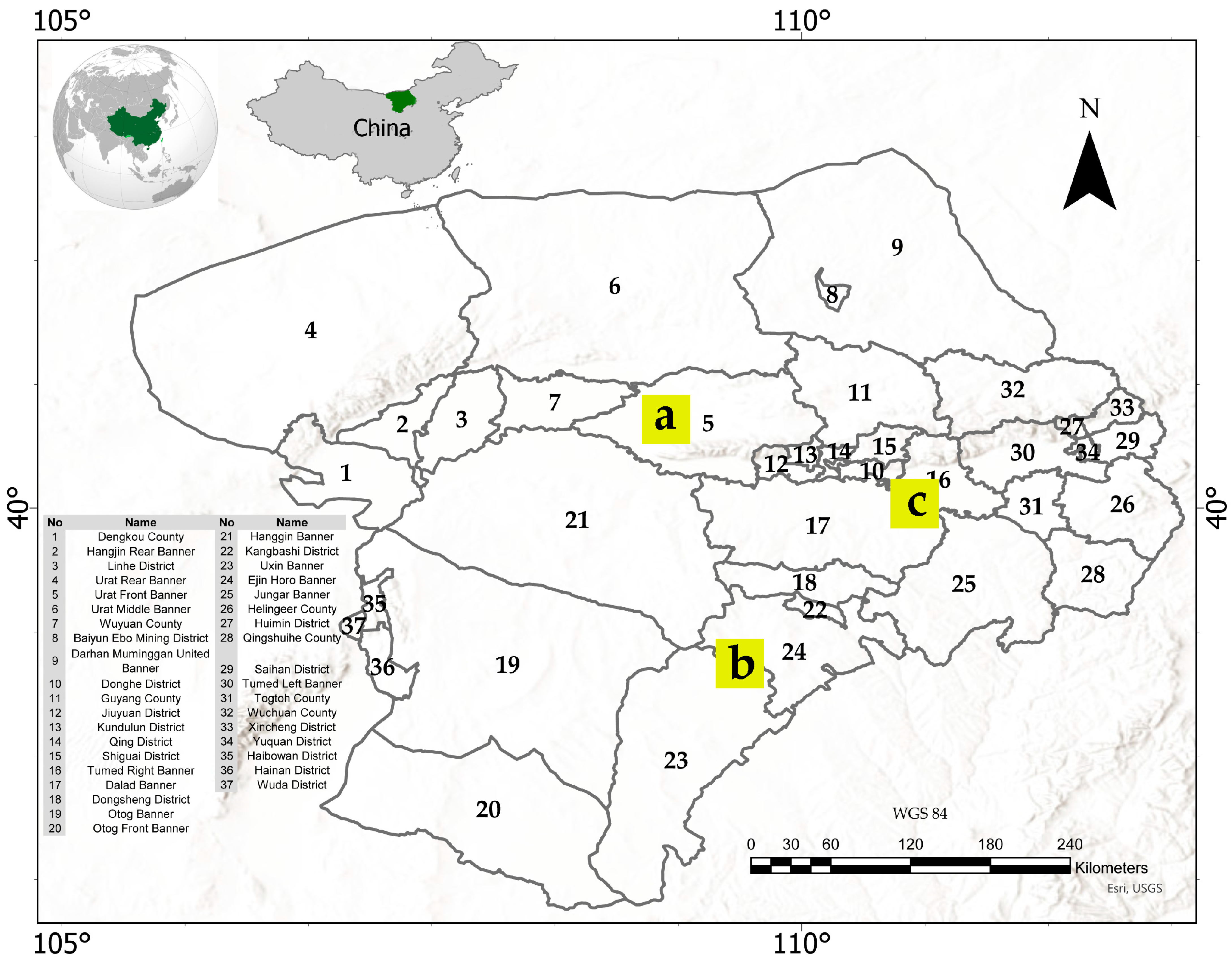
Figure 1. (a–c) Location of the study area, highlighting three representative regions analyzed in detail for land use/land cover changes.
Remotesensing 17 01089 g001
Figure 2. Flowchart of the research methodology.
Remotesensing 17 01089 g002
Figure 3. Taylor diagram for climate model comparison: (a) temperature and (b) precipitation in the study area.
Remotesensing 17 01089 g003
Figure 4. (a) Trends in annual temperature and (b) trends in annual precipitation from 1980 to 2100 in the study area.
Remotesensing 17 01089 g004
Figure 5. Spatial distribution of annual precipitation (top row) and temperature (bottom row) during the base period and under future scenarios (SSP2-4.5 and SSP5-8.5) for 2030–2050.
Remotesensing 17 01089 g005
Figure 6. Comparison of consumer and producer accuracy for land use classes, overall accuracy, and Kappa statistics.
Remotesensing 17 01089 g006
Figure 7. (ac) Land use maps of the study area for the years 2007, 2023, and 2040, illustrating spatial changes and transitions over time. The numbers represent sub-basins, as explained in Figure 1.
Remotesensing 17 01089 g007
Figure 8. Localized (ac) views of land use/land cover classifications in 2007, 2023, and 2040, illustrating wetland changes in three representative areas within the broader study region. The locations of these areas (ac) are indicated in Figure 1.
Remotesensing 17 01089 g008
Figure 9. (a) Gain and loss charts and (b) net changes in land use, including (c) net changes in herbaceous wetlands (2007–2023).
Remotesensing 17 01089 g009
Figure 10. (a) Gain and loss charts and (b) net changes in land use, including (c) net changes in herbaceous wetlands (2023–2040).
Remotesensing 17 01089 g010
Figure 11. Losses in herbaceous wetlands (2007–2023).
Remotesensing 17 01089 g011
Figure 12. Additional key environmental variables used in the MaxEnt model show the (a) elevation, (b) slope, (c) landforms, and (d) soil texture. The numbers represent sub-basins, as explained in Figure 1.
Remotesensing 17 01089 g012
Figure 13. Probability of wetland distribution under future conditions (scenarios SSP245 and SSP585). The numbers represent sub-basins, as explained in Figure 1.
Remotesensing 17 01089 g013
Table 2. Characteristics of selected GCMs.
ModelInstitutionNominal ResolutionPrimary Reference
ACCESS-CM2Commonwealth Scientific and Industrial Research Organisation (CSIRO), Australia~1.875° × 1.25°[48]
CNRM-CM6-1Centre National de Recherches Météorologiques (CNRM), France~1.4° × 1.4°[49]
CNRM-ESM2-1Centre National de Recherches Météorologiques (CNRM), France~1.4° × 1.4°[50]
MPI-ESM1-2-HRMax Planck Institute for Meteorology (MPI), Germany~0.9° × 0.9°[51]
MRI-ESM2-0Meteorological Research Institute (MRI), Japan~1.125° × 1.125°[52]
UKESM1-0-LLMet Office Hadley Centre, UK~1.25° × 1.875°[53]
Table 3. Identified land cover types in the study area [29].
ClassLand Use TypeDescription
1Herbaceous vegetationPlants without persistent stems or shoots above ground and lacking a definite firm structure. Tree and shrub cover is less than 10%.
2Cultivated and managed vegetation/agricultureLands covered with temporary crops followed by harvest and a bare soil period (e.g., single and multiple cropping systems).
3Urban/built-upLand covered by buildings and other man-made structures.
4Bare/sparse vegetationLands with exposed soil, sand, or rocks that never have a vegetated cover of more than 10% during any time of the year.
5Permanent water bodiesLakes, reservoirs, and rivers. Can be either fresh or salt water bodies.
6Herbaceous wetlandLands with a permanent mixture of water and herbaceous or woody vegetation. The vegetation can be present in either salt, brackish, or fresh water.
7ForestIncludes all forest types (evergreen and deciduous, needleleaf and broadleaf, open and closed). These areas have tree canopies ranging from 15% to >70%.
Table 4. Pearson’s correlation matrix (entire study area).
Land_CoverNDVILandformElevationHumidityPrecipitationRadiationSlopeMean_TempMax_TempMin_Temp
Land_Cover1−0.520.12−0.21−0.62−0.590.250.080.070.080.06
NDVI−0.521−0.130.110.630.72−0.30.10.05−0.030.13
Landform0.12−0.131−0.15−0.18−0.170.03−0.130−0.010.02
Elevation−0.210.11−0.1510.180.210.050.35−0.52−0.51−0.52
Humidity−0.620.63−0.180.1810.9−0.660.09−0.28−0.33−0.22
Precipitation−0.590.72−0.170.210.91−0.370.1−0.01−0.070.05
Radiation0.25−0.30.030.05−0.66−0.3710.010.550.60.49
Slope0.080.1−0.130.350.090.10.011−0.19−0.19−0.18
Mean_Temp0.070.050−0.52−0.28−0.010.55−0.1910.990.99
Max_Temp0.08−0.03−0.01−0.51−0.33−0.070.6−0.190.9910.96
Min_Temp0.060.130.02−0.52−0.220.050.49−0.180.990.961
Disclaimer/Publisher’s Note: The statements, opinions and data contained in all publications are solely those of the individual author(s) and contributor(s) and not of MDPI and/or the editor(s). MDPI and/or the editor(s) disclaim responsibility for any injury to people or property resulting from any ideas, methods, instructions or products referred to in the content.