Technical Note

Spatial Regionalization of the Arctic Ocean Based on Ocean Physical Property

Center of Remote Sensing & GIS, Korea Polar Research Institute, Incheon 21990, Republic of Korea
*
Author to whom correspondence should be addressed.
Remote Sens. 2025, 17(6), 1065; https://doi.org/10.3390/rs17061065
Submission received: 27 January 2025 / Revised: 10 March 2025 / Accepted: 14 March 2025 / Published: 18 March 2025
(This article belongs to the Section Ocean Remote Sensing)

Abstract

:
The Arctic Ocean has a uniquely complex system associated with tightly coupled ocean–ice–atmosphere–land interactions. The Arctic Ocean is considered to be highly susceptible to global climate change, with the potential for dramatic environmental impacts at both regional and global scales, and its spatial differences particularly have been exacerbated. A comprehensive understanding of Arctic Ocean environmental responses to climate change thus requires classifying the Arctic Ocean into subregions that describe spatial homogeneity of the clusters and heterogeneity between clusters based on ocean physical properties and implementing the regional-scale analysis. In this study, utilizing the long-term optimum interpolation sea surface temperature (SST) datasets for the period 1982–2023, which is one of the essential indicators of physical processes, we applied the K-means clustering algorithm to generate subregions of the Arctic Ocean, reflecting distinct physical characteristics. Using the variance ratio criterion, the optimal number of subregions for spatial clustering was 12. Employing methods such as information mapping and pairwise multi-comparison analysis, we found that the 12 subregions of the Arctic Ocean well represent spatial heterogeneity and homogeneity of physical properties, including sea ice concentration, surface ocean currents, SST, and sea surface salinity. Spatial patterns in SST changes also matched well with the boundaries of clustered subregions. The newly identified physical subregions of the Arctic Ocean will contribute to a more comprehensive understanding of the Arctic Ocean’s environmental response to accelerating climate change.

1. Introduction

The Arctic Ocean exhibits unique features and complex dynamics characterized by a confluence of various water masses, circulation dynamics, and seasonal ice cover (Figure 1) [1]. In recent decades, the Arctic has warmed almost four times faster than the rest of the globe, referred to as Arctic amplification [2,3,4]. It is believed that this amplification is caused by complex physical mechanisms, including local feedback (e.g., temperature and sea ice-related feedback) and changes in poleward energy transport (e.g., poleward ocean heat transport through the Atlantic and Pacific Ocean gateways) [5]. In particular, a reduction in sea ice has been shown to be a primary cause of spatial disparities in Arctic warming [6,7], with maximum warming in the Barents–Kara Seas where the sea ice loss was most pronounced [8,9]. Advection of anomalous Atlantic and Pacific waters into the Arctic Ocean (called atlantification and pacification, respectively) has also contributed to warming and contrasting regional differences in stratification, with the strengthening of stratification in the Amerasian Basin but weakening in the Eurasian Basin, potentially altering nutrient fluxes and primary production [1,10,11,12]. Therefore, a better understanding of the Arctic Ocean’s response to accelerating climate change requires regional-scale comprehensive analysis. Spatial clustering defining distinct ocean physical characteristics will provide a more accurate and environmentally consistent representation of important features over the Arctic Ocean compared to one unit (entire area) or uniform grids.
The subregions of the Arctic Ocean have been mainly classified according to the international standards described by the International Hydrographic Organization (IHO) [13] and National Snow and Ice Data Center (NSIDC), based on oceanic bathymetric features and geographic and sea ice characteristics, respectively [14,15]. While these definitions of delineating regions have been accepted to be useful for an application to hydrographic surveys and to sea-ice research [1,16,17], there may be limitations in separating the Arctic Ocean regions, where the complex processes that intertwine sea ice and ocean dynamics occur, based on these definitions [15]. Sea ice acts as a crucial mediator of atmosphere–ocean momentum transfer that drives surface ocean circulation, but the recent reduction in sea ice has led to ice-free areas in the Arctic Ocean, having a substantial impact on oceanic mixing [18,19]. Moreover, Arctic sea ice loss is projected to occur regardless of the region and season [20]. Besides the decrease in sea ice, the Arctic Ocean has been experiencing recent drastic changes that include increased intensity and frequency of extreme ocean events, such as marine heatwaves (MHWs), which have the potential for profound ecological impacts [21,22,23,24]. Spatial classification of the Arctic Ocean will thus require considering the temporal and spatial variability of oceanographic parameters that are inextricably linked to climate change rather than sea ice or geographic features.
Sea surface temperature (SST) is one of the key indicators for evaluating climate systems, regulating the interactions between the ocean and the atmosphere, and exchanging heat, gases, and moisture [25]. The SST data have been frequently used as a significant physical quantity to study and understand both ocean physical and biogeochemical processes. They also reveal climate change as an essential climate variable [26,27]. Understanding the variability of SST in the Arctic Ocean is particularly necessary for understanding changes in water column stratification, nutrient flux, and primary production [28]. The fluctuations in SST provide valuable insights into regional and long-term shifts in Arctic Ocean conditions, making it a crucial parameter for identifying dynamic subregions of the Arctic [29,30]. In addition, the gap-filled SST datasets, combining in situ and satellite data, offer a more precise and comprehensive approach to studying ocean physical processes that require high temporal and spatial resolution [31,32].
Therefore, specifically, this study aimed to generate a robust regionalization of the Arctic Ocean (north of the Arctic Circle; >66.6°N) that describes distinct characteristics of ocean physical properties based on a gap-filled SST dataset produced using an optimum interpolation (OI) technique [31]. The OISST-derived subregions were mapped over the Arctic Ocean. Furthermore, spatial overlap with a regionalization was used to validate that clustered subregions are internally homogeneous and heterogeneous between subregions based on ocean physical variables, and mean comparison analysis was applied to evaluate clustering performance in terms of heterogeneity between clusters.

2. Data and Methods

2.1. Datasets

For clustering analysis, this study used the National Oceanic and Atmospheric Administration (NOAA) long-term OISST daily dataset for the period 1982–2023, version 2.1, which is a blend of in situ and satellite SSTs derived from the Advanced Very High Resolution Radiometer (AVHRR) [31,32]. AVHRR SSTs were bias corrected by adjusting them relative to in situ buoy observations at 0.2 m nominal depth from the International Comprehensive Ocean–Atmosphere Data Set (ICOADS) near-real-time (NRT) release (R3.0.2) [33]. In the ice-covered regions (ice concentration >35%), OISST v2.1 data have significant quality improvements by applying a freezing point based on climatological sea surface salinity (SSS) instead of regressed ice–SST proxy, which results in a warm bias, used in OISST v2.0 [34]. Daily SST values on a 25 km rectangular grid were re-gridded onto a 25 km polar stereographic grid using the nearest interpolation method. We have computed the annual mean of SST for the same period. The data are available at https://www.ncei.noaa.gov/products/optimum-interpolation-sst (accessed on 17 March 2025).
The classification performance of subregions defined in this study was evaluated based on ocean physical parameters, including sea ice concentration (SIC), surface current, SST, and SSS datasets, which are essential variables to understand the physical properties of the Arctic Ocean. The separated datasets, distinct from the clustering dataset, were needed to measure the performance of clustering results accurately. The monthly SIC data were derived from the NSIDC dataset, which is generated from the Nimbus-7 Scanning Multichannel Microwave Radiometer (SMMR), Defence Meteorological Satellite Program (DMSP)-F8, -F11, and -F13 Special Sensor Microwave/Imagers (SSM/Is), and the DMSP-F17 Special Sensor Microwave Imager/Sounder (SSMIS) (NSIDC-0051, https://nsidc.org/data/NSIDC-0051, accessed on 17 March 2025) [35]. These datasets have a spatial resolution of 25 km × 25 km with the polar-stereographic grid. Climatological monthly SIC data were calculated by averaging the monthly maps for 1982–2023. For the performance evaluation on clustered subregions, we also used climatological monthly mean fields of SST, SSS, and surface currents data (1993–2023) derived from the Copernicus Marine Environment Monitoring Service (CMEMS)-Global Ocean Ensemble Reanalysis product, which is available at https://data.marine.copernicus.eu/product/GLOBAL_MULTIYEAR_PHY_ENS_001_031/description (accessed on 17 March 2025) [36]. These data were obtained through an oceanic numerical model constrained by assimilating satellites and in situ observations. These products were on a 0.25° Earth grid and re-gridded onto a 25 km polar stereographic grid.

2.2. Methods

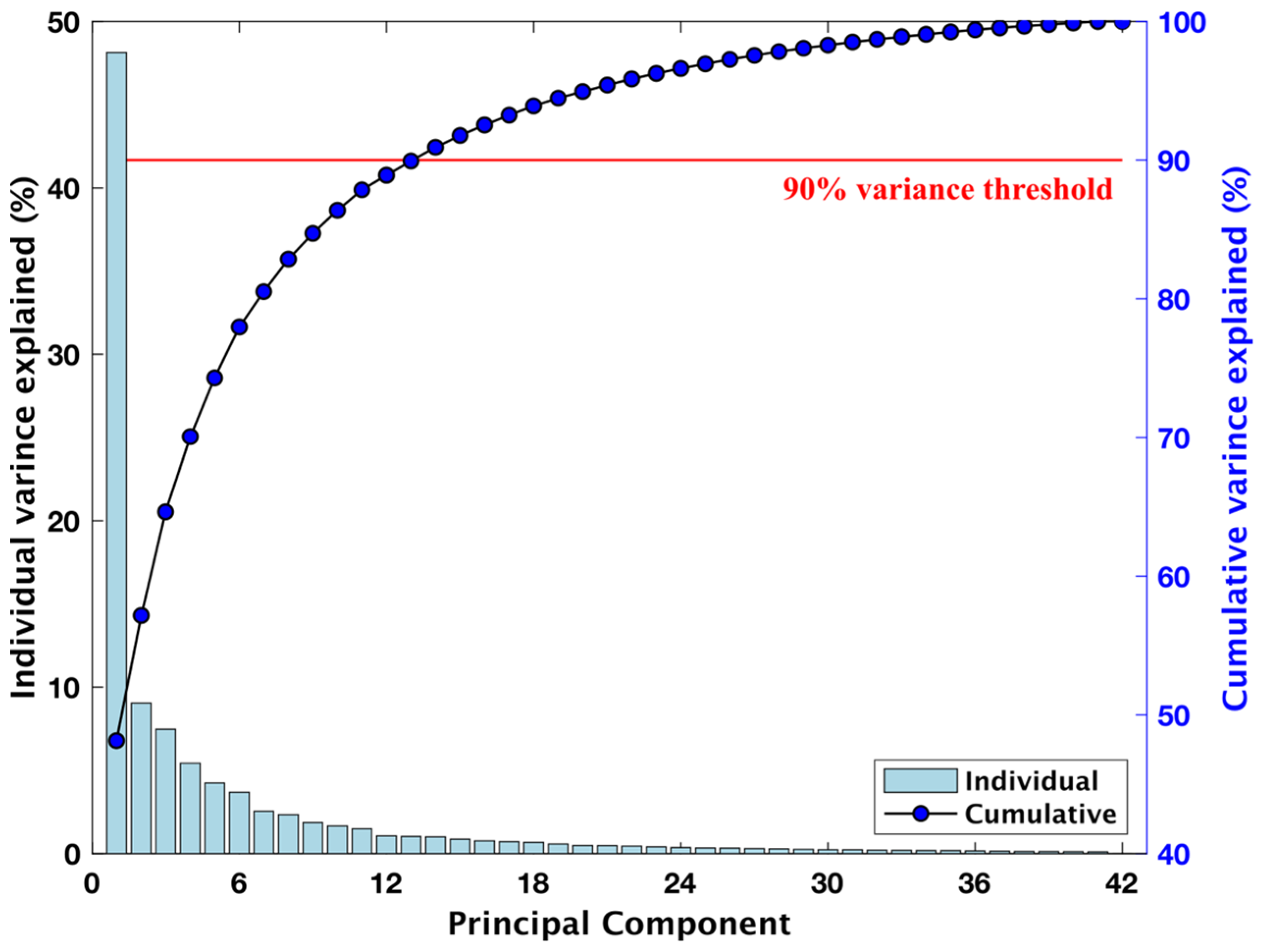
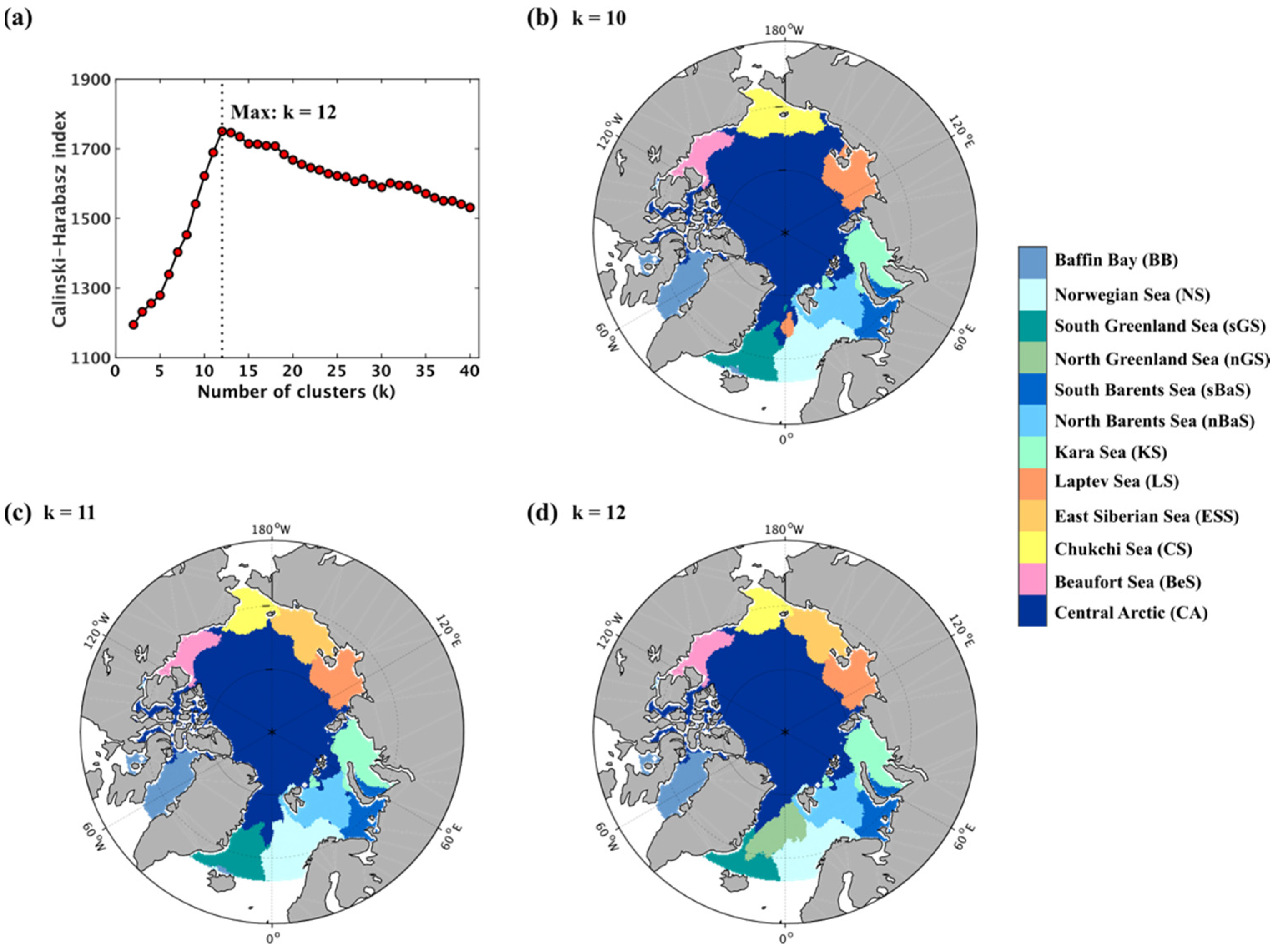
2.2.1. Subregion Clustering Methods

Figure 2 presents a schematic diagram of the clustering analysis procedure used to classify the Arctic Ocean into subregions, each distinguished by distinctive physical characteristics, based on the OISST dataset. The procedure consisted of two steps: data pre-processing and regional clustering.
To avoid incorrect identification in cluster analysis, a surface-type flag from NOAA NSIDC was first applied [15]. We masked out invalid pixels on all collected data corresponding to non-ocean regions, including land, freshwater, land ice, ice shelf, and disconnected ocean. We removed the land-contaminated pixels around the shorelines (up to 25 km from the coast).
In order to extract the dominant pattern of SST variability in the Arctic Ocean, we also performed principal component analysis (PCA) as a data pre-processing step before the clustering analysis. PCA is a statistical method that allows a reduction in data complexity and enhances interpretability by focusing on the most significant features and eliminating redundancy and error [37,38]. This study applied PCA to determine the dominant patterns of residual variance in the SST dataset. The spatiotemporal SST dataset, S S T   x ,   t can be decomposed into two matrices, as shown in Equation (1) [39]:
S S T   x ,   t = j = 1 N E O F j x   P C j t
where E O F j x represents eigen functions and   P C j t are their temporal amplitudes, with N being the number of modes.
The number of significant features in a dataset was determined by considering “rules of thumb”, retaining the components that capture 90% of the cumulative explained variance [40]. Significant SST features extracted from PCA analysis were used as input variables for clustering analysis.
The second step was to perform a clustering technique for regionalization. We employed the K-means clustering algorithm, one of the most popular and straightforward unsupervised learning algorithms [41]. The K-means algorithm aims to partition unlabeled data points into k clusters by minimizing the sum of squared distances between each data point and the corresponding cluster centroid [42]. This method starts by randomly selecting k data points as the initial set of centroids, and the performance quality depends primarily on the initialization technique. To minimize clustering errors made by K-means, we applied an improved cluster initialization method called K-means++ [43]. Instead of choosing a centroid randomly, the K-means++ algorithm selects the initial centroids using distance calculations based on their proximity to each point. The K-means algorithm has also been reported to work well with a repeat strategy, showing a substantial reduction in clustering errors by repeating the algorithm 100 times [44]. We performed K-means 100 times, starting with different initializations (Figure 2).
The optimal k number of clusters was evaluated based on the clustering validity index, Calinski–Harabasz (CH) index, also known as the variance ratio criterion, the most commonly used evaluation metric for clustering solution [45,46,47]. This index measures the ratio of the sum of inter-cluster dispersion and the sum of intra-cluster dispersion for all clusters. The CH index for k different clusters is defined as follows [45]:
C H = k = 1 K n k C k C 2 K 1   /   k = 1 K i = 1 n k X i k C k 2 N K
where N is the total number of data points, K is the number of clusters, n k and C k are the number of points and centroid of the cluster k, respectively, C is the centroid of the dataset, and X i k is the i-th data point belonging to the cluster k.
The CH index is higher when the clusters are dense and well-separated, and the highest CH index was selected as the optimal number of clusters for a K-means clustering algorithm.
Lastly, using the traditional cutoff probability of 0.05, we removed the outliers, i.e., cluster points beyond the threshold corresponding to the 95th percentile of the square root of the sum of the squared distances from the data point to the centroid of their assigned cluster. After removing outliers, missing values were interpolated using the nearest-neighbor method.

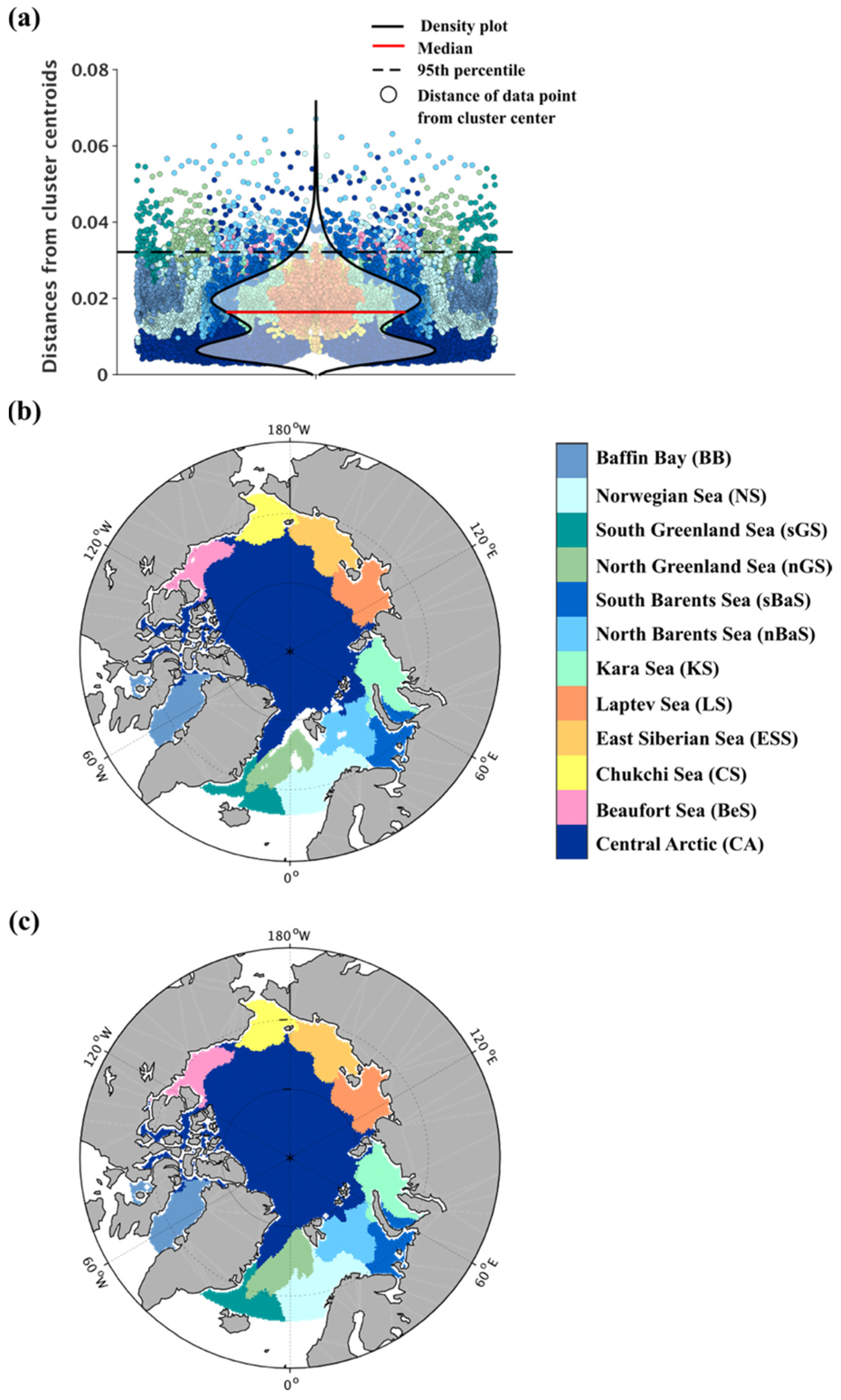
2.2.2. Evaluation of the Performance of the Classified Subregions

The one-way analysis of variance (one-way ANOVA) is a statistical method to aggregate differences among the k group means (k > 2) [48]. In ANOVA, the null hypothesis is that there is no difference among group means. We conducted a one-way ANOVA to test a statistically significant difference between the mean values of ocean physical variables from subregions identified in this study. The ANOVA table captures an F-statistic, the ratio of the mean square between groups (between-group variance) divided by the mean square within groups (within-group variance). The mean squares are derived from the mean of the sum of squares. To further explore which group mean or means are statistically different in physical variables, we performed the Tukey test for multiple comparisons, comparing all possible pairwise combinations of each group mean [49]. Tukey’s honest significance test is accomplished by presenting 95% confidence intervals for all pairwise differences between group means.

3. Results and Discussion

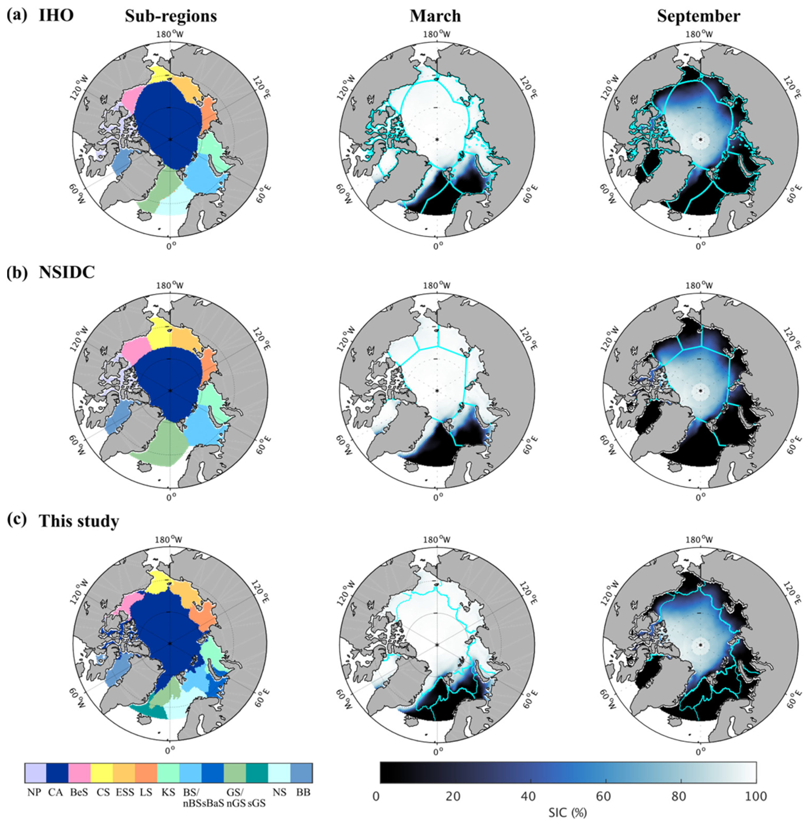
3.1. K-Means Based Regionalization of the Arctic Ocean Using the SST Dataset

The regionalization of the Arctic Ocean was conducted based on the significant variances in the annual SST dataset (Figure 2). The high and variable noise levels in the datasets may confound the image analysis unless properly handled [50]. Thus, as the data pre-processing step before cluster analysis, the significant temporal–spatial signals in the annual SST datasets were extracted based on the PCA analysis, which separates the signal information from noise [37,38]. PCA transforms the original variables into a new set of variables called principal components (PCs), which are ordered in decreasing order of importance. We considered a 90% level of the cumulative percent of variance as a rule-of-thumb cutoff for determining how many PCs are significant, which is a common threshold to retain components [40]. Figure 3 depicts the individual and cumulative variances explained by the PCs. The black line with the blue circle represents the cumulative variance explained, while the red line represents the 90% threshold for selecting the number of PCs to retain. A cutoff criterion of 90% resulted in the first 14 PCs, indicating 14 PCs will cumulatively account for more than 90% of the total variance of the SST dataset.
Next, using the subset of 14 PCs produced from the 42-year annual SST dataset, we performed the regional clusters of the Arctic Ocean based on the K-means++ algorithm, one of the most widely used and simple clustering algorithms in the regionalization analysis [51,52]. The performance of K-means clustering was evaluated by comparing the number of clusters, ranging from k = 2 to k = 40 (Figure 4). According to the quantitative CH criterion, the optimal number of clusters for the Arctic Ocean subregions occurred at 12 clusters, which correspond to the greatest CH value, reflecting the maximum separability, i.e., within-cluster similarity and between-clusters difference (Figure 4a). The 12 Arctic subregions classified through K-means clustering were defined as follows (Figure 4d): Central Arctic (CA), Beaufort Sea (BeS), Chukchi Sea (CS), East Siberian Sea (ESS), Laptev Sea (LS), Kara Sea (KS), north Barents Sea (nBaS), south Barents Sea (sBaS), north Greenland Sea (nGS), south Greenland Sea (sGS), Norwegian Sea (NS), and Baffin Bay (BB). The spatial displays of subregions clustered into ten to eleven are shown in Figure 4b,c. Regardless of the number of clusterings, the subregions clustered through K-means identified BeS, LS, KS, nBaS, sBaS, NS, and BB regions as separate groups, indicating that these regions are more coherent and homogenous than other regions. The difference between 10 subregions and 11 to 12 subregions was CS and ESS, which were grouped together in 10 subregions. The 12 subregions showed higher classification in the areas influenced by Atlantic waters than the 10 to 11 subregions. In particular, the CA defined by 12 subregions included the areas along the coast of Northeast Greenland, which is characterized by year-round sea ice [53].
As previous studies showed that K-means++ algorithm captures spatial coherence, avoiding spatially disconnected clusters [54,55,56], most pixels were clustered into distinct regional labels, showing clear-cut boundaries, but there were mixed labels in the areas, mainly around Svalbard, indicating incorrect classification (Figure 4d). The Fram Strait and around north of Svalbard have been characterized by spatially inhomogeneous surface conditions, resulting from highly dynamic sea-ice conditions and complex bathymetry [57,58,59]. To identify and remove these mislabeled data points, we applied the outliers adopting the 95th percentile thresholds of distances (>0.0322) (Figure 5a). All outliers, including mixed labels around Svalbard, were treated as mislabeled data samples and removed from the classification (Figure 5b). Finally, to deal with the uncertainty of removed attributes in clusters, each extracted point was replaced by the nearest neighboring data point according to the nearest-neighborhood interpolation method (Figure 5c). This procedure allowed for aggregating similar spatial entities together into regions.

3.2. Evaluation of Subregional Classification Results for the Arctic Ocean
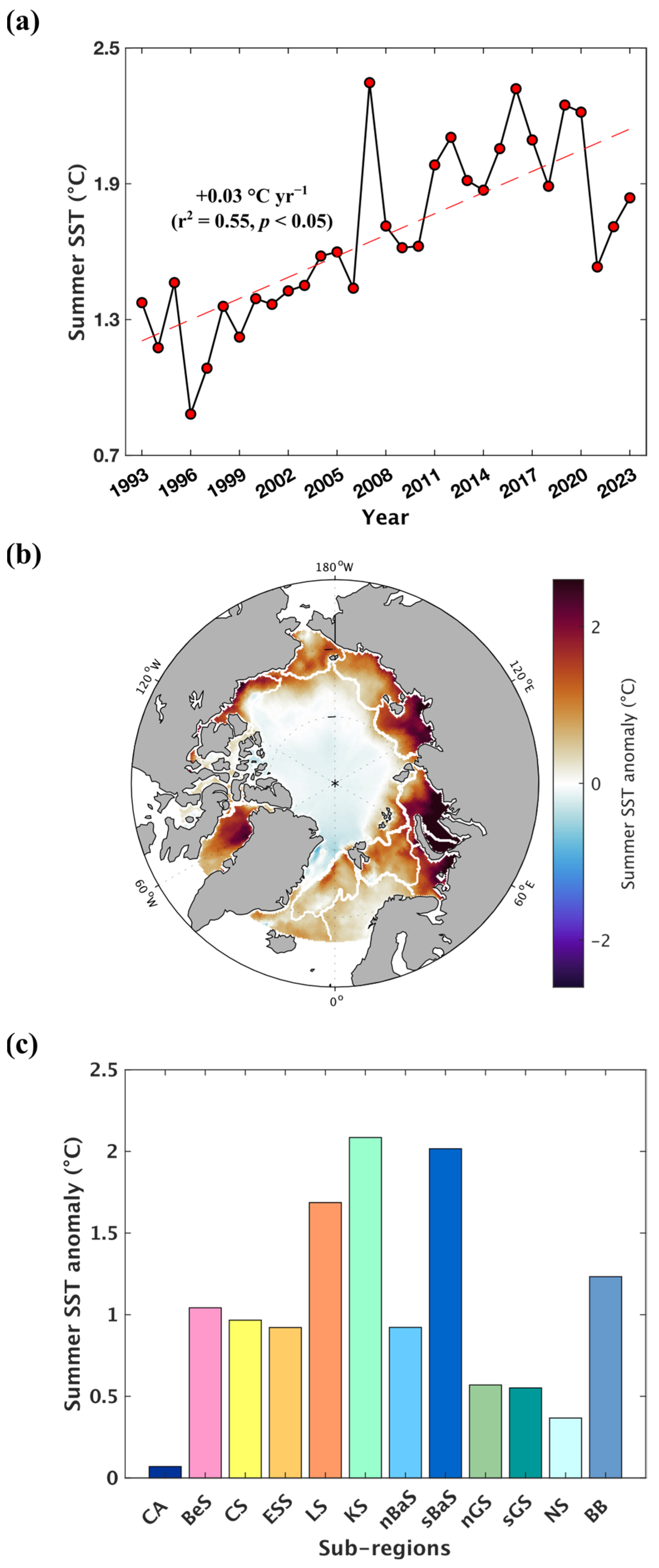
In this section, we evaluated the performance of 12 subregions (Figure 5c) in the intra-cluster homogeneity and inter-cluster heterogeneity based on the physical characteristics of the Arctic Ocean: SIC, surface currents, SST, and SSS. In particular, the sea ice almost entirely covers the Arctic Ocean during winter, and during summer it retreats off the shallow water [60]. The presence and variation in sea ice significantly influence the ocean circulation pattern and physical and biogeochemical parameters in the Arctic Ocean. Therefore, the spatial heterogeneity was first examined by overlaying classified subregions, given each definition (IHO, NSIDC, and this study), on the spatial maps of climatological mean SIC in March and September (Figure 6). The spatial map of climatological mean SIC showed maximum sea ice extent in March, while minimum sea ice extent in September. For the northern limit of the Pacific sector (BeS, CS, ESS, and LS), NSIDC definition was northward of boundaries in IHO and this study, as NSIDC boundaries were set as lines of constant latitude and longitude for simplicity (Figure 6a,b) [15]. The Pacific sector boundaries of this study followed the distribution of nearly ice-free open water in September, displaying a similar extent with IHO defined from bathymetry (Figure 6a,c) [13]. It supports that ocean seafloor features control warm and cold surface waters, dictating the sea ice dynamics [61]. On the other hand, IHO and NSIDC definitions separated the CA cluster from the Northwest Passage (NP) cluster, and the Atlantic sector limit of the CA cluster was defined by the northernmost point of Greenland and Svalbard Island (GS and BaS) (Figure 6a,b) [13,14,15]. However, in both months, high SIC values (>~60%) were distributed over the central parts of the Arctic Ocean to the northeastern coast of Greenland and the NP, indicating that IHO and NSIDC have limitations in drawing these covers of sea ice, but consistent with the boundary of CA cluster specified in this study (Figure 6c). The CA cluster in this study also corresponds to perennial (two or more years old) ice-covered areas where sea ice exists for 95% or more of the year [53].
Secondly, we investigated the performance of classified subregions based on the spatial maps of winter (December to February) and summer (July to September) mean averages of reanalysis-based surface currents, SST, and SSS, which represent the physical features of the Arctic Ocean, between 1993 and 2023 (Figure 7). The circulation in the Arctic Ocean is dynamically driven by the wind and by thermohaline caused by cooling/heating and freshening/salinification [62]. Both seasons captured two dominant wind-driven circulation features: Beaufort gyre and Transpolar drift (Figure 1 and Figure 7a). The anticyclonic high-pressure system over the Canada Basin, called Beaufort High, forces the Beaufort gyre circulation [63]. The extent of Beaufort gyre circulation corresponded to BeS and CS margins specified in this study (Figure 7a). The Transpolar Drift current is driven by the pressure gradients near the surface between the Canada and Eurasian basins and transports ice and fresh water from both the eastern Siberian shelves and the Beaufort Gyre across the central Arctic toward Greenland [64,65]. The extent of areas with high SIC around Greenland (Figure 6c) followed the patterns of Transpolar Drift, bounding the CA region, which is homogeneously cold and fresh (Figure 7a–c). In the winter season, ice-covered areas, besides CA, were physically distinguished from ice-free areas, showing relatively cold (SST: −1.7––1.5 °C) and fresh conditions (SSS: 27.2–31.9) (Figure 6c and Figure 7b,c).
Climatological ocean physical features also described well the inflows from the Pacific and Atlantic waters, representing visually distinct clusters. Inflow current (northward flow) from the warm and saline Pacific Ocean through the Bering Strait was distributed over the CS region, bounded on the north by the Beaufort gyre and Chukchi Sea Slope Current (Figure 7a). During the ice-free summer season, the CS region was visually separated from BeS, ESS, and CA regions (i.e., the areas surrounding CS) by a relatively high temperature (3.5 °C) and high salinity upper layer (30) (Figure 7b,c). The Norwegian Atlantic Current mainly carried the inflow of warm and saline Atlantic water to the Arctic Ocean through the NS, as defined in this study (Figure 1 and Figure 7a). The dominant northward flow was observed in the NS, distinguished from nGS and sGS regions, with the warmest and saltiest water in both seasons, and this flow was advected via the two branches in the northern part of NS: the eastern branch through the sBaS and western branch through Fram Strait. The sBaS region was characterized by ~1.5 times higher SST values in response to relatively stronger northeastward advection of Atlantic water compared to the nBaS region. It is consistent with the findings of previous studies that the warm inflows keep sBaS ice-free throughout the year and increase air–sea interactions [66]. These physical differences between north and south in the BaS led to the distribution of fish communities dominated by Arctic species in nBaS but boreal species in sBaS [67]. Accordingly, this regionalization is more suitable for depicting Arctic Ocean surface conditions than IHO and NSIDC classifications that defined BaS as one group (Figure 6a,b). The waters advected from Atlantic water moved farther east along the Eurasian Coast, reaching the KS and LS [62].
The Arctic Ocean is a strongly river-influenced ocean, catching greater than 10% of global river discharge [68]. The BeS, ESS, LS, and KS predominantly receive a large amount of relatively warm freshwater from five major rivers (Mackenzie, Kolyma, Yenisey, Lena, and Ob rivers), forming a plume of low salinity warm waters (Figure 1 and Figure 7c). Over these areas, there were relatively lower salinity waters in the summer than in the winter, with peak river discharge in summer [69]. In particular, the KS (Yenisey and Ob Rivers) and LS (Lena River) receive about one-half of the total river runoff during the ice-free periods, and the Lena River plume from the LS is constantly spreading to ESS region [70].
On the other hand, the ESS region showed distinct characteristics with slow surface currents and low SST patterns, distinguished from surrounding areas (CS and LS). The relatively slow current was also distributed over the nGS bounded by the cold East Greenland Current and warm West Spitsbergen Current, which are southward-flowing and northward-flowing, respectively (Figure 7a). This region formed mixed physical properties. In particular, the Svalbard Archipelago has captured the signature of Atlantification, a process associated with anomalous Atlantic Water inflows over the last two decades, inducing uncertainties in physical and ecological changes [11,71]. Along Greenland’s east coast, there was a meridional gradient in climatological SIC values, decreasing to the south, as divided along the coast of GS, separating sGS (Figure 6c). The sGS was characterized by southward flowing cold East Greenland Current and East Icelandic Current (Figure 7a).
These results indicated that the OISST-derived subregions identified in this study were well classified, reflecting the surface circulation pattern, which determines the spatial patterns of temperature and salinity.
Further, using the climatological mean values of reanalysis-derived SST and SSS for the winter and summer seasons, the difference between the 12 subregional groups was statistically compared. To assess variations in SST and SSS among the subregions, we first applied one-way ANOVA (Table 1). The null hypothesis was that there was no difference in the averages across the 12 subregions based on each set of climatological mean SST or SSS values averaged for winter and summer seasons. The ANOVA results rejected the null hypothesis in all variables, with a p-value (Prob > F) of 0.00 (p < 0.05) (Table 1). It concludes that there is a statistical difference across the subregional SST and SSS averages for winter and summer, providing a validity of dividing 12 subregions.
As the ANOVA test is limited to understanding which group or groups differ from the others, we also carried out the multiple pairwise comparison test, commonly used to test significant differences in all possible pairs of each group mean [72]. Figure 8 and Tables S1–S4 show the results of the pairwise comparison test based on the Tukey pairwise mean with 95% confidence intervals that assess the significance of differences among 12 subregions, indicating that the group means are significantly different if their shaded areas (95% confidence intervals of the mean) are disjointed (p < 0.05). In winter, due to the influence of the ice cover (Figure 6c), the confidence intervals of climatological winter mean SST values were overlapped for the entire Arctic Ocean except for the areas influenced by Atlantic water (Figure 8a and Table S1), suggesting SST values in the ice-covered regions are not statistically different at the 5% level. However, even in winter, there were significant differences in means between nBaS and sBaS and between nGS and sGS, supporting the physical suitability of this classification compared to IHO and NSIDC. Furthermore, during the summer, climatological mean SST values represented statistically distinct regional differences in all possible pairs between 12 subregions (Figure 8a and Table S2). These results support that clustered groups in this study were well determined to depict the spatial heterogeneity of SST values. The climatological winter and summer mean SSS values also varied between 12 subregions (Figure 8b and Tables S3 and S4). The SSS values in 12 subregions indicated the spatial patterns, being grouped mainly into three zones: strong salinity zone influenced by Atlantic water (nBaS, sBaS, nGS, sGS, and NS), low salinity zone strongly influenced by river discharge (BeS, ESS, and LS), and saline-fresh water mixed zone (CA, CS, KS, and BB). In both seasons, differences in mean SSS values between adjacent regions were also significant, with disjoint confidence intervals for the mean values, but during summer, there was no significant difference between ESS and LS and between nGS and sGS, as shown in Figure 7c. Overall, the results demonstrated that 12 subregions statistically differ significantly in physical variables, indicating a robust regionalization.

3.3. Implications

During ice-free periods, the Arctic Ocean SST has increased at a rate of 0.03 °C yr−1 since the 1993 year (r2 = 0.55, p < 0.05) (Figure 9a). As shown in the Arctic sea ice [73], there was a clear shift in summer Arctic SST in the 2007 year. The spatial difference in summer SST anomalies of 2007 to 2023 relative to 1993 to 2006 was quite substantial among the 12 subregions, with relatively higher SST values in BeS, LS, KS, sBaS, and BB (Figure 9b,c). These spatial patterns matched well with the boundaries of subregions clustered in this study, indicating accelerated regional-scale warming. A recent study has reported that a dramatic increase in Pacific waters has a strong connection with wind-driven processes, while ocean heat transport through the Atlantic gate strongly affected the BaS and KS [74]. Furthermore, the Arctic Ocean amplification under global warming has also been found with a substantial regional difference, showing prominent warming in the BaS and KS [74,75]. Several studies revealed that the occurrence of MHWs in the Arctic Ocean has markedly increased over the past 40 years, comparable with the global average [21,23], and in a future warming climate, the occurrence of MHWs and its impact are anticipated to be much more potent compared to others [76]. As the localized extreme events could potentially exert an even more substantial impact on the Arctic Ocean ecosystem, future studies are needed to understand not only the spatial–temporal pattern dynamics of the extreme events in the Arctic Ocean (e.g., MHW) but also their influencing factors and driving mechanisms based on the physically well-defined subregions. Thus, these results will contribute to a better understanding of the Arctic Ocean’s changing dynamics induced by extreme climate events, capturing subregional representative changes characterized by distinct regional dynamics.

4. Conclusions

Because of the complex environmental system over the Arctic Ocean, a robust regionalization based on the physical characteristics of the ocean is an essential step in understanding and predicting the response of the Arctic Ocean environment to accelerated warming. SST is a fundamental physical property that can directly or indirectly affect the climate and marine ecosystems. Based on the long-term annual mean NOAA OISST data for 1982–2023, we aimed to address a spatial regionalization of the Arctic Ocean that describes physical characteristics using the unsupervised K-means++ clustering algorithm. The 12 spatial subregions have been identified by different SST regimes based on the CH index. Using minimum and maximum SIC distribution, we showed that OISST-derived regionalization captured more of the physical characteristics on a regional scale compared to IHO and NSIDC. Using the climatological values of reanalysis-derived ocean surface current, SST, and SSS that represent significant physical properties for winter and summer seasons, we also presented that the subregions defined with OISST changes were effective at a clear and distinct suite of physical conditions over the Arctic Ocean, indicating distinct regional dynamics in surface current, SST, and SSS by each region. Additionally, this regionalization captured unique spatial differences in the summer SST changes, matching well with the boundaries of subregions clustered in this study. Further investigation is needed for the detailed integration of the physical and biological characteristics and their underlying mechanisms in each region of the Arctic Ocean. The application of this regionalization will also aid in achieving a more comprehensive understanding of the spatial and temporal heterogeneity in climate change effects on the Arctic Ocean environments.

Supplementary Materials

The following supporting information can be downloaded at https://www.mdpi.com/article/10.3390/rs17061065/s1, Tables S1–S4: Multiple comparison results of the climatological mean SST and SSS during winter and summer seasons.

Author Contributions

Conceptualization, J.-E.Y. and H.-C.K.; Data curation, J.-E.Y.; Funding acquisition, H.-C.K.; Investigation, J.-E.Y.; Methodology, J.-E.Y., J.P. and H.-C.K.; Visualization: J.-E.Y.; Supervision, H.-C.K.; Writing—Original draft, J.-E.Y.; Writing—review and editing, J.-E.Y., J.P. and H.-C.K. All authors have read and agreed to the published version of the manuscript.

Funding

This research was funded by the Korea Polar Research Institute, grant number PE25040.

Data Availability Statement

All data used in this study can be obtained by contacting the corresponding author via email.

Acknowledgments

We thank the editor and reviewers for their comments on this paper.

Conflicts of Interest

The authors declare no conflicts of interest.

References

  1. Timmermans, M.-L.; Marshall, J. Understanding Arctic Ocean Circulation: A Review of Ocean Dynamics in a Changing Climate. J. Geophys. Res. Ocean. 2020, 125, e2018JC014378. [Google Scholar] [CrossRef]
  2. Rantanen, M.; Karpechko, A.Y.; Lipponen, A.; Nordling, K.; Hyvärinen, O.; Ruosteenoja, K.; Vihma, T.; Laaksonen, A. The Arctic has warmed nearly four times faster than the globe since 1979. Commun. Earth Environ. 2022, 3, 168. [Google Scholar] [CrossRef]
  3. England, M.R.; Eisenman, I.; Lutsko, N.J.; Wagner, T.J.W. The Recent Emergence of Arctic Amplification. Geophys. Res. Lett. 2021, 48, e2021GL094086. [Google Scholar] [CrossRef]
  4. Jansen, E.; Christensen, J.H.; Dokken, T.; Nisancioglu, K.H.; Vinther, B.M.; Capron, E.; Guo, C.; Jensen, M.F.; Langen, P.L.; Pedersen, R.A.; et al. Past perspectives on the present era of abrupt Arctic climate change. Nat. Clim. Chang. 2020, 10, 714–721. [Google Scholar] [CrossRef]
  5. Previdi, M.; Smith, K.L.; Polvani, L.M. Arctic amplification of climate change: A review of underlying mechanisms. Environ. Res. Lett. 2021, 16, 093003. [Google Scholar] [CrossRef]
  6. Dai, A.; Luo, D.; Song, M.; Liu, J. Arctic amplification is caused by sea-ice loss under increasing CO2. Nat. Commun. 2019, 10, 121. [Google Scholar] [CrossRef]
  7. Screen, J.A.; Simmonds, I. The central role of diminishing sea ice in recent Arctic temperature amplification. Nature 2010, 464, 1334–1337. [Google Scholar] [CrossRef]
  8. Isaksen, K.; Nordli, Ø.; Ivanov, B.; Køltzow, M.A.Ø.; Aaboe, S.; Gjelten, H.M.; Mezghani, A.; Eastwood, S.; Førland, E.; Benestad, R.E.; et al. Exceptional warming over the Barents area. Sci. Rep. 2022, 12, 9371. [Google Scholar] [CrossRef]
  9. Lind, S.; Ingvaldsen, R.B.; Furevik, T. Arctic warming hotspot in the northern Barents Sea linked to declining sea-ice import. Nat. Clim. Change 2018, 8, 634–639. [Google Scholar] [CrossRef]
  10. Polyakov, I.V.; Alkire, M.B.; Bluhm, B.A.; Brown, K.A.; Carmack, E.C.; Chierici, M.; Danielson, S.L.; Ellingsen, I.; Ershova, E.A.; Gårdfeldt, K.; et al. Borealization of the Arctic Ocean in Response to Anomalous Advection From Sub-Arctic Seas. Front. Mar. Sci. 2020, 7, 491. [Google Scholar] [CrossRef]
  11. Polyakov, I.V.; Pnyushkov, A.V.; Alkire, M.B.; Ashik, I.M.; Baumann, T.M.; Carmack, E.C.; Goszczko, I.; Guthrie, J.; Ivanov, V.V.; Kanzow, T.; et al. Greater role for Atlantic inflows on sea-ice loss in the Eurasian Basin of the Arctic Ocean. Science 2017, 356, 285–291. [Google Scholar] [CrossRef] [PubMed]
  12. Woodgate, R.A. Increases in the Pacific inflow to the Arctic from 1990 to 2015, and insights into seasonal trends and driving mechanisms from year-round Bering Strait mooring data. Prog. Oceanogr. 2018, 160, 124–154. [Google Scholar] [CrossRef]
  13. International Hydrographic Organization. Limits of Oceans and Seas; International Hydrographic Organization: Monaco, 1953. [Google Scholar]
  14. Parkinson, C.L.; Cavalieri, D.J.; Gloersen, P.; Zwally, H.J.; Comiso, J.C. Arctic sea ice extents, areas, and trends, 1978–1996. J. Geophys. Res. Ocean. 1999, 104, 20837–20856. [Google Scholar] [CrossRef]
  15. Meier, W.; Stewart, J. Arctic and Antarctic Regional Masks for Sea Ice and Related Data Products; version 1; NASA National Snow and Ice Data Center Distributed Active Archive Center: Boulder, CO, USA, 2023.
  16. Peng, G.; Meier, W.N. Temporal and regional variability of Arctic sea-ice coverage from satellite data. Ann. Glaciol. 2018, 59, 191–200. [Google Scholar] [CrossRef]
  17. Wang, Z.; Li, Z.; Zeng, J.; Liang, S.; Zhang, P.; Tang, F.; Chen, S.; Ma, X. Spatial and temporal variations of Arctic Sea Ice from 2002–2017. Earth Space Sci. 2020, 7, e2020EA001278. [Google Scholar] [CrossRef]
  18. Kikuchi, T.; Nishino, S.; Fujiwara, A.; Onodera, J.; Yamamoto-Kawai, M.; Mizobata, K.; Fukamachi, Y.; Watanabe, E. Status and trends of Arctic Ocean environmental change and its impacts on marine biogeochemistry: Findings from the ArCS project. Polar Sci. 2021, 27, 100639. [Google Scholar] [CrossRef]
  19. Rainville, L.; Lee, C.M.; Woodgate, R.A. Impact of wind-driven mixing in the Arctic Ocean. Oceanography 2011, 24, 136–145. [Google Scholar] [CrossRef]
  20. Årthun, M.; Onarheim, I.H.; Dörr, J.; Eldevik, T. The Seasonal and Regional Transition to an Ice-Free Arctic. Geophys. Res. Lett. 2021, 48, e2020GL090825. [Google Scholar] [CrossRef]
  21. Huang, B.; Wang, Z.; Yin, X.; Arguez, A.; Graham, G.; Liu, C.; Smith, T.; Zhang, H.-M. Prolonged Marine Heatwaves in the Arctic: 1982−2020. Geophys. Res. Lett. 2021, 48, e2021GL095590. [Google Scholar] [CrossRef]
  22. Carmack, E.; Polyakov, I.; Padman, L.; Fer, I.; Hunke, E.; Hutchings, J.; Jackson, J.; Kelley, D.; Kwok, R.; Layton, C.; et al. Toward Quantifying the Increasing Role of Oceanic Heat in Sea Ice Loss in the New Arctic. Bull. Am. Meteorol. Soc. 2015, 96, 2079–2105. [Google Scholar] [CrossRef]
  23. Barkhordarian, A.; Nielsen, D.M.; Olonscheck, D.; Baehr, J. Arctic marine heatwaves forced by greenhouse gases and triggered by abrupt sea-ice melt. Commun. Earth Environ. 2024, 5, 57. [Google Scholar] [CrossRef]
  24. Smale, D.A.; Wernberg, T.; Oliver, E.C.J.; Thomsen, M.; Harvey, B.P.; Straub, S.C.; Burrows, M.T.; Alexander, L.V.; Benthuysen, J.A.; Donat, M.G.; et al. Marine heatwaves threaten global biodiversity and the provision of ecosystem services. Nat. Clim. Change 2019, 9, 306–312. [Google Scholar] [CrossRef]
  25. Emery, W.J. AIR–SEA INTERACTION|Sea Surface Temperature. In Encyclopedia of Atmospheric Sciences; Holton, J.R., Ed.; Academic Press: Amsterdam, The Netherlands, 2003; pp. 100–109. [Google Scholar]
  26. Stocker, T. Climate Change 2013: The Physical Science Basis: Working Group I Contribution to the Fifth Assessment Report of the Intergovernmental Panel on Climate Change; Cambridge University Press: Cambridge, UK, 2014. [Google Scholar]
  27. Merchant, C.J.; Embury, O.; Bulgin, C.E.; Block, T.; Corlett, G.K.; Fiedler, E.; Good, S.A.; Mittaz, J.; Rayner, N.A.; Berry, D.; et al. Satellite-based time-series of sea-surface temperature since 1981 for climate applications. Sci. Data 2019, 6, 223. [Google Scholar] [CrossRef]
  28. Lenn, Y.-D.; Fer, I.; Timmermans, M.-L.; MacKinnon, J.A. Chapter 11—Mixing in the Arctic Ocean. In Ocean Mixing; Meredith, M., Naveira Garabato, A., Eds.; Elsevier: Amsterdam, The Netherlands, 2022; pp. 275–299. [Google Scholar]
  29. Carvalho, K.; Wang, S. Sea surface temperature variability in the Arctic Ocean and its marginal seas in a changing climate: Patterns and mechanisms. Glob. Planet. Change 2020, 193, 103265. [Google Scholar] [CrossRef]
  30. Behera, P.; Tiwari, M.; Knies, J. Enhanced Arctic Stratification in a Warming Scenario: Evidence From the Mid Pliocene Warm Period. Paleoceanogr. Paleoclimatol. 2021, 36, e2020PA004182. [Google Scholar] [CrossRef]
  31. Reynolds, R.W.; Smith, T.M.; Liu, C.; Chelton, D.B.; Casey, K.S.; Schlax, M.G. Daily High-Resolution-Blended Analyses for Sea Surface Temperature. J. Clim. 2007, 20, 5473–5496. [Google Scholar] [CrossRef]
  32. Huang, B.; Liu, C.; Banzon, V.; Freeman, E.; Graham, G.; Hankins, B.; Smith, T.; Zhang, H.-M. Improvements of the Daily Optimum Interpolation Sea Surface Temperature (DOISST), Version 2.1. J. Clim. 2021, 34, 2923–2939. [Google Scholar] [CrossRef]
  33. Liu, C.; Freeman, E.; Kent, E.C.; Berry, D.I.; Worley, S.J.; Smith, S.R.; Huang, B.; Zhang, H.-M.; Cram, T.; Ji, Z.; et al. Blending TAC and BUFR Marine In Situ Data for ICOADS Near-Real-Time Release 3.0.2. J. Atmos. Ocean. Technol. 2022, 39, 1943–1959. [Google Scholar] [CrossRef]
  34. Banzon, V.; Smith, T.M.; Steele, M.; Huang, B.; Zhang, H.-M. Improved Estimation of Proxy Sea Surface Temperature in the Arctic. J. Atmos. Ocean. Technol. 2020, 37, 341–349. [Google Scholar] [CrossRef]
  35. DiGirolamo, N.; Parkinson, C.; Cavalieri, D.; Gloersen, P.; Zwally, H. Sea Ice Concentrations from Nimbus-7 SMMR and DMSP SSM/I-SSMIS Passive Microwave Data, version 2; NASA National Snow and Ice Data Center Distributed Active Archive Center: Boulder, CO, USA, 2022. [Google Scholar]
  36. Copernicus Marine Service. Global Ocean Ensemble Physics Reanalysis, Marine Data Store (MDS) [Data Set]. 2023. Available online: https://doi.org/10.48670/moi-00024 (accessed on 17 March 2025).
  37. Jackson, J.E. A User’s Guide to Principal Components; John Wiley & Sons: Hoboken, NJ, USA, 2005. [Google Scholar]
  38. Jolliffe, I.T.; Cadima, J. Principal component analysis: A review and recent developments. Philos. Trans. A Math. Phys. Eng. Sci. 2016, 374, 20150202. [Google Scholar] [CrossRef]
  39. Lorenz, E.N. Empirical Orthogonal Functions and Statistical Weather Prediction; Massachusetts Institute of Technology, Department of Meteorology: Cambridge, MA, USA, 1956; Volume 1. [Google Scholar]
  40. Jolliffe, I.T. Principal Component Analysis; Springer: Berlin/Heidelberg, Germany, 2002. [Google Scholar]
  41. MacQueen, J. Some methods for classification and analysis of multivariate observations. In Proceedings of the 5th Berkeley Symposium on Mathematical Statistics and Probability; University of California Press: Berkeley, CA, USA, 1967. [Google Scholar]
  42. Lloyd, S. Least squares quantization in PCM. IEEE Trans. Inf. Theory 1982, 28, 129–137. [Google Scholar] [CrossRef]
  43. Arthur, D.; Vassilvitskii, S. K-Means++: The Advantages of Careful Seeding. In Proceedings of the Eighteenth Annual ACM-SIAM Symposium on Discrete Algorithms, New Orleans, LA, USA, 7–9 January 2007; Volume 8, pp. 1027–1035. [Google Scholar]
  44. Fränti, P.; Sieranoja, S. How much can k-means be improved by using better initialization and repeats? Pattern Recognit. 2019, 93, 95–112. [Google Scholar] [CrossRef]
  45. Caliński, T.; Ja, H. A Dendrite Method for Cluster Analysis. Commun. Stat. Theory Methods 1974, 3, 1–27. [Google Scholar] [CrossRef]
  46. Milligan, G.W.; Cooper, M.C. An examination of procedures for determining the number of clusters in a data set. Psychometrika 1985, 50, 159–179. [Google Scholar] [CrossRef]
  47. Patil, C.; Baidari, I. Estimating the Optimal Number of Clusters k in a Dataset Using Data Depth. Data Sci. Eng. 2019, 4, 132–140. [Google Scholar] [CrossRef]
  48. Hogg, R.V.; Ledolter, J. Engineering Statistics; Macmillan: New York, NY, USA, 1987. [Google Scholar]
  49. Hochberg, Y.; Tamhane, A.C. Multiple Comparison Procedures; Wiley: Hoboken, NJ, USA, 1987. [Google Scholar]
  50. Razifar, P.; Muhammed, H.H.; Engbrant, F.; Svensson, P.E.; Olsson, J.; Bengtsson, E.; Långström, B.; Bergström, M. Performance of principal component analysis and independent component analysis with respect to signal extraction from noisy positron emission tomography data—A study on computer simulated images. Open Neuroimag. J. 2009, 3, 1–16. [Google Scholar] [CrossRef]
  51. Jain, A.K. Data clustering: 50 years beyond K-means. Pattern Recognit. Lett. 2010, 31, 651–666. [Google Scholar] [CrossRef]
  52. Hartigan, J.A.; Wong, M.A. Algorithm AS 136: A K-Means Clustering Algorithm. J. R. Stat. Soc. Ser. C Appl. Stat. 1979, 28, 100–108. [Google Scholar] [CrossRef]
  53. Wang, X.; Liu, Y.; Key, J.R.; Dworak, R. A New Perspective on Four Decades of Changes in Arctic Sea Ice from Satellite Observations. Remote Sens. 2022, 14, 1846. [Google Scholar] [CrossRef]
  54. Aguilar Colmenero, J.L.; Portela Garcia-Miguel, J. A Regionalization Approach Based on the Comparison of Different Clustering Techniques. Appl. Sci. 2024, 14, 10563. [Google Scholar] [CrossRef]
  55. Mendler, F.; Koch, B.; Meißner, B.; Voglstätter, C.; Smolinka, T. Evaluation of spatial clustering methods for regionalisation of hydrogen ecosystems. Energy Strategy Rev. 2025, 57, 101627. [Google Scholar] [CrossRef]
  56. Anselin, L. An Introduction to Spatial Data Science with GeoDa; Taylor & Francis: Abingdon, UK, 2024; Volume 1: Exploring Spatial Data. [Google Scholar]
  57. Dahlke, S. Rapid Climate Changes in the Arctic Region of Svalbard Aktuelle Klimaänderungen in der Svalbard-Region. Ph.D. Thesis, University of Potsdam, Potsdam, Germany, 2020. [Google Scholar]
  58. Watkins, D.M.; Bliss, A.C.; Hutchings, J.K.; Wilhelmus, M.M. Evidence of Abrupt Transitions Between Sea Ice Dynamical Regimes in the East Greenland Marginal Ice Zone. Geophys. Res. Lett. 2023, 50, e2023GL103558. [Google Scholar] [CrossRef]
  59. Kozlov, I.E.; Atadzhanova, O.A. Eddies in the Marginal Ice Zone of Fram Strait and Svalbard from Spaceborne SAR Observations in Winter. Remote Sens. 2022, 14, 134. [Google Scholar] [CrossRef]
  60. Ravindran, S.; Pant, V.; Mitra, A.K.; Kumar, A. Spatio-temporal variability of sea-ice and ocean parameters over the Arctic Ocean in response to a warming climate. Polar Sci. 2021, 30, 100721. [Google Scholar] [CrossRef]
  61. Nghiem, S.V.; Clemente-Colón, P.; Rigor, I.G.; Hall, D.K.; Neumann, G. Seafloor control on sea ice. Deep. Sea Res. Part. II Top. Stud. Oceanogr. 2012, 77–80, 52–61. [Google Scholar] [CrossRef]
  62. Rudels, B.; Carmack, E. Arctic Ocean Water Mass Structure and Circulation. Oceanography 2022, 35, 52–65. [Google Scholar] [CrossRef]
  63. Serreze, M.C.; Barrett, A.P. Characteristics of the Beaufort Sea High. J. Clim. 2011, 24, 159–182. [Google Scholar] [CrossRef]
  64. Thorndike, A.S.; Colony, R. Sea ice motion in response to geostrophic winds. J. Geophys. Res. Ocean. 1982, 87, 5845–5852. [Google Scholar] [CrossRef]
  65. Colony, R.; Thorndike, A. An estimate of the mean field of Arctic sea ice motion. J. Geophys. Res. Ocean. 1984, 89, 10623–10629. [Google Scholar] [CrossRef]
  66. Long, Z.; Perrie, W. Changes in Ocean Temperature in the Barents Sea in the Twenty-First Century. J. Clim. 2017, 30, 5901–5921. [Google Scholar] [CrossRef]
  67. Ingvaldsen, R.; Assmann, K.; Primicerio, R.; Fossheim, M.; Polyakov, I.; Dolgov, A. Physical manifestations and ecological implications of Arctic Atlantification. Nat. Rev. Earth Environ. 2021, 2, 874–889. [Google Scholar] [CrossRef]
  68. McClelland, J.W.; Holmes, R.M.; Dunton, K.H.; Macdonald, R.W. The Arctic Ocean Estuary. Estuaries Coasts 2012, 35, 353–368. [Google Scholar] [CrossRef]
  69. Gibson, G.A.; Elliot, S.; Clement Kinney, J.; Piliouras, A.; Jeffery, N. Assessing the Potential Impact of River Chemistry on Arctic Coastal Production. Front. Mar. Sci. 2022, 9, 738363. [Google Scholar] [CrossRef]
  70. Osadchiev, A.A.; Pisareva, M.N.; Spivak, E.A.; Shchuka, S.A.; Semiletov, I.P. Freshwater transport between the Kara, Laptev, and East-Siberian seas. Sci. Rep. 2020, 10, 13041. [Google Scholar] [CrossRef]
  71. Bensi, M.; Nilsen, F.; Ferre, B.; Skogseth, R.; Moskalik, M.; Korhonen, M.; Vogedes, D.; Kovacevic, V.; Paladini, F.; Ingrosso, G.; et al. The Atlantification process in Svalbard: A broad view from the SIOS Marine Infrastructure network. In SESS Report 2024: Svalbard Integrated Arctic Earth Observing System; Runge, E., Neuber, R., Łupikasza, E., Hübner, C., Holmén, K., Eds.; Svalbard Integrated Arctic Earth Observing System (SIOS): Longyearbyen, Norway, 2025; pp. 138–151. [Google Scholar]
  72. Jaccard, J.; Becker, M.; Wood, G. Pairwise multiple comparison procedures: A review. Psychol. Bull. 1984, 96, 589–596. [Google Scholar] [CrossRef]
  73. Sumata, H.; de Steur, L.; Divine, D.V.; Granskog, M.A.; Gerland, S. Regime shift in Arctic Ocean sea ice thickness. Nature 2023, 615, 443–449. [Google Scholar] [CrossRef]
  74. Li, Z.; Ding, Q.; Steele, M.; Schweiger, A. Recent upper Arctic Ocean warming expedited by summertime atmospheric processes. Nat. Commun. 2022, 13, 362. [Google Scholar] [CrossRef]
  75. Kumar, A.; Yadav, J.; Mohan, R. Spatio-temporal change and variability of Barents-Kara sea ice, in the Arctic: Ocean and atmospheric implications. Sci. Total Environ. 2021, 753, 142046. [Google Scholar] [CrossRef]
  76. He, Q.; Zhu, Z.; Zhao, D.; Song, W.; Huang, D. An Interpretable Deep Learning Approach for Detecting Marine Heatwaves Patterns. Appl. Sci. 2024, 14, 601. [Google Scholar] [CrossRef]
Figure 1. Schematic circulation of Arctic Ocean. The bathymetric contours are shown, and the arrows refer to Pacific currents (green), Atlantic currents (red), other currents (blue), and river outflow (cyan).
Remotesensing 17 01065 g001
Figure 2. Flow chart working on the spatial regionalization of the Arctic Ocean.
Remotesensing 17 01065 g002
Figure 3. Individual (sky-blue bar) and cumulative (black line with blue circle) explained variances for determining how many principal components to retain. The red line indicates the 90% variance threshold.
Remotesensing 17 01065 g003
Figure 4. Subregional classification of the Arctic Ocean based on K-means clustering analysis: (a) CH index plot for two up to 40 groups. The highest CH index value (dotted black line) corresponds to the optimal number of clusters; (bd) Maps of the 10–12 subregions obtained through K-means clustering. The 12 subregions are as follows: Central Arctic (CA), Beaufort Sea (BeS), Chukchi Sea (CS), East Siberian Sea (ESS), Laptev Sea (LS), Kara Sea (KS), north Barents Sea (nBaS), south Barents Sea (sBaS), north Greenland Sea (nGS), south Greenland Sea (sGS), Norwegian Sea (NS), and Baffin Bay (BB).
Remotesensing 17 01065 g004
Figure 5. Classification of the Arctic Ocean with outlier removal: (a) a violin plot overlaid the swarm plot for distributions of cluster distances. The dotted line indicates the 95th percentile threshold of the distances. The color indicates subregions; the violin plot depicts the kernel density estimate of the data, and the swarm plot displays individual data points in a way that no points are overlapping; (b) Map of 12 clustered subregions that outliers were excluded (>95th percentile of the distances); (c) Final map of 12 clustered subregions after nearest-neighbor interpolation.
Remotesensing 17 01065 g005
Figure 6. The climatological map of SIC for March (center) and September (right) overlaid with subregions clustered (left) from (a) IHO, (b) NSIDC, and (c) this study. The subregions are as follows: Northwest Passage (NP), Central Arctic (CA), Beaufort Sea (BeS), Chukchi Sea (CS), East Siberian Sea (ESS), Laptev Sea (LS), Kara Sea (KS), Barents Sea (BaS)/north Barents Sea (nBaS), south Barents Sea (sBaS), Greenland Sea (GS)/north Greenland Sea (nGS), south Greenland Sea (sGS), Norwegian Sea (NS), and Baffin Bay (BB).
Remotesensing 17 01065 g006
Figure 7. The climatological maps of (a) surface current, (b) SST, and (c) SSS averaged for winter (left) and summer season (right) overlaid with subregions clustered in this study.
Remotesensing 17 01065 g007
Figure 8. Pairwise comparison of the confidence intervals of the climatological mean (a) SST and (b) SSS during the winter (left) and summer seasons (right) by subregions defined in this study. The circle marker indicates the mean value. Each shaded area with a vertical black line represents a 95% confidence interval of the mean value, indicating that the group means are significantly different if their confidence intervals (shaded area with a vertical black line) are disjointed. Color indicates subregions (as shown in Figure 5c).
Remotesensing 17 01065 g008
Figure 9. The temporal variation in Summer SST in the Arctic Ocean. (a) Time series of summer SST values averaged for the entire Arctic Ocean. The red dashed line indicates a fitted linear regression line with a slope of 0.03 °C yr−1 (r2 = 0.55, p < 0.05). (b) Spatial distribution of the difference in summer mean SST between the period of 2007 to 2023 and the period of 1993 to 2006. The white segments correspond to 12 subregions. (c) Subregional summer mean SST anomalies during the periods of 2007 to 2023 relative to the periods of 1993 to 2006. Color indicates subregions (as shown in Figure 5c).
Remotesensing 17 01065 g009
Table 1. One-way ANOVA statistical analysis for climatological mean SST and SSS in winter and summer for the 12 subregions.
VariableSource of
Variation
Sum of SquaresDegree of FreedomMean SquaresF-Ratiop-Value
(Prob > F)
Winter
SST
Between groups64,186.9115835.29599.10.00
Within groups10,914.717,9550.61
Total75,101.517,966
Summer
SST
Between groups181,942.51116,540.210,530.50.00
Within groups28,201.817,9551.6
Total210,144.217,966
Winter
SSS
Between groups80,615.5117328.73329.50.00
Within groups39,521.417,9552.2
Total120,136.917,966
Summer
SSS
Between groups165,154.41115,014.03532.30.00
Within groups76,316.817,9554.25
Total241,471.217,966
Disclaimer/Publisher’s Note: The statements, opinions and data contained in all publications are solely those of the individual author(s) and contributor(s) and not of MDPI and/or the editor(s). MDPI and/or the editor(s) disclaim responsibility for any injury to people or property resulting from any ideas, methods, instructions or products referred to in the content.

