Synthetic Aperture Radar Processing Using Flexible and Seamless Factorized Back-Projection

Abstract

This paper describes a flexible and seamless processor for Unmanned Aerial Vehicle (UAV)-borne Synthetic Aperture Radar (SAR) imagery. When designing a focusing algorithm for large-scale and high-resolution SAR images, efficiency and accuracy are two mandatory aspects to consider. The proposed processing scheme is based on a modified version of Fast Factorized Back-Projection (FFBP), in which the factorization procedure is interrupted on the basis of a computational cost analysis to reduce the number of complex operations at its minimum. The algorithm gains efficiency in the case of low-altitude platforms, where there are significant variations in azimuth resolution, but not in the case of conventional airborne missions, where the azimuth resolution can be considered constant in the swath. The algorithm’s performance is derived by assessing the number of complex operations required to focus an SAR image. Two scenarios are tackled in a numerical simulation: a UAV-borne SAR with a short synthetic aperture and a wide field of view, referred to as the ground-based-like (GBL) scenario, and a classical stripmap scenario. In both cases, we consider mono-static and bi-static radar configurations. The results of the numerical simulations show that the proposed algorithm outperforms FFBP in the stripmap scenario while achieving the same performance as FFBP in the GBL scenario. In addition, the algorithm is validated thanks to an experimental UAV-borne SAR campaign in the X-band.

1. Introduction

Synthetic Aperture Radar (SAR) is a well-known high-resolution electromagnetic imagery technique. It allows flexible observation of an area of interest due to its ability to produce all-weather day-and-night imagery. In recent years, Unmanned Aerial Vehicle (UAV) technology has gained interest from the scientific community. For example, significant technological advances [1] have opened up the potential of Unmanned Aerial Vehicles (UAVs) for a wide range of applications. For example, in [2], the UAV is addressed as an aerial wireless platform to provide better coverage and enhanced sensing and communication services. Additionally, drones have moved into the mass market, which has decreased costs and made drone network deployment much more cost effective [3]. UAVs can be a valuable asset for SAR due to their easy deployment, agile trajectory planning, and high maneuverability. Some interesting applications are mine detection and clearance [4,5], Earth observation [6,7,8], and search-and-rescue applications [9,10,11]. Some drawbacks of this technology are the low battery capacity and payload restriction regarding size, weight, and power consumption. In addition, the highly non-linear trajectories typically traveled by UAVs are generally complex to handle during SAR focusing. Thus, focusing schemes relying on straight trajectory assumptions are not possible, for instance, the $\omega -k$ [12] or a Range-Doppler algorithm [13]. In fact, the UAV-SAR system requires a time-domain focusing scheme, as described in [14,15,16,17,18,19]. Typically, a time-domain focusing technique comes with a downside: its computational complexity scales linearly with the data size. Thus, it is slower compared to frequency-domain focusing techniques.

However, some techniques that tackle the computational burden have been developed in the literature, such as Fast Factorized Back-Projection (FFBP) [20]. The main idea behind FFBP is that the entire aperture is divided into sub-apertures that are focused separately, leading to several low-resolution images. These images are then merged coherently step by step until the entire trajectory is processed and one full-resolution image is produced. The FFBP algorithm has been exploited in the literature due to its low computational burden [21,22,23]. In our work, we define two scenarios as the two extreme cases of our application. The first is ground-based-like (GBL) UAV SAR with a trajectory in the order of tens of meters and a wide antenna aperture to enlighten a wide area. The second is a classical stripmap scenario with a wide trajectory that covers the area of interest.

We aim to define a flexible and versatile processor operating in both scenarios with minimal computational cost. This algorithm is meant to gain computational speed using a low-altitude platform with a wide swath, where the azimuth resolution varies significantly in a single swath. In contrast, the computational advantage is not significant compared to airborne missions using high-altitude platforms, as, for instance, in [24]. Moreover, our algorithm has been compared to FFBP in such a wide scenario that an overlap-and-add technique is required. The entire processing chain is described in detail, including the ad hoc reference system developed to increase the efficiency of the back-projection. Performances regarding the rough number of operations required to focus an SAR image are derived. Some guidelines are derived from these performances for efficiently implementing the entire workflow. Then, a numerical analysis to quantify the computational burden is proposed. Afterward, a numerical simulation is provided to the reader in order to evaluate the algorithm’s accuracy. Ultimately, the algorithm is validated using an off-the-shelf UAV and customized radar equipment operating in the X-band. Section 2 encompasses the signal model and describes Time-Domain Back-Projection (TDBP) and Fast Factorized Back-Projection. Section 3 is the core of our work and describes the proposed focusing scheme with a complete computational cost analysis. Section 4 describes the two scenarios of our application, and Section 5 draws a numerical comparison between FFBP and our algorithm. Finally, Section 6 shows real data results from an X-band experimental campaign, and, in Section 7, the conclusions are drawn.

2. Signal Model and Conventional Time-Domain Focusing Schemes

In this section, we will describe the signal model and the two focusing techniques: Time-Domain Back-Projection (TDBP) and Fast Factorized Back-Projection (FFBP).

2.1. Time-Domain Back-Projection

After the range compression, the signal model for a bi-static radar is no different from the mono-static one, as described in [25]:

$$\begin{array}{c}\hfill s(t;{\mathbf{p}}_0,{\tau }_n)\propto \sin \mathrm{c}\left[{\displaystyle \frac{t-\overline{t}({\mathbf{p}}_0,{\tau }_n)}{{\rho }_t}}\right]\times \exp \left\{-j2\pi f_0\overline{t}({\mathbf{p}}_0,{\tau }_n)\right\}\end{array}$$

(1)

where t is the fast-time variable, ${\tau }_n$ is the slow-time variable associated with the platform movement, and ${\rho }_t$ is the time resolution defined as ${\rho }_t=1/B$, where B is the signal bandwidth. ${\mathbf{p}}_0={[x_0,y_0,z_0]}^{\mathrm{T}}$ is a generic target position vector, $f_0$ is the transmitter central frequency, and $\overline{t}({\mathbf{p}}_0,{\tau }_n)$ is the two-way travel time, intended as the delay between the transmitter to the target and back to the receiver. Time-Domain Back-Projection (TDBP) is assumed to carry out signal focusing to cope with non-linear trajectories. It consists of a mathematical operator that performs the coherent sum of the phase-shifted acquired data:

$$\begin{array}{c}\hfill I\left(\mathbf{p}\right)=\sum _{n=1}^{N_{\tau }}w({\rho }_{az},\mathbf{p},{\tau }_n)s(t=\overline{t}(\mathbf{p},{\tau }_n))\exp \left\{j2\pi f_0\overline{t}\left(\mathbf{p}\right)\right\}\end{array}$$

(2)

where $\overline{t}(\mathbf{p},{\tau }_n)$ is the delay taken by the signal to travel from the Tx antenna to a generic pixel in $\mathbf{p}$, and from $\mathbf{p}$ to the Rx antenna. Finally, $N_{\tau }$ is the number of slow-time samples to be back-projected to obtain the desired resolution. In Equation (2), some spectral weights $w({\rho }_{az},\mathbf{p},{\tau }_n)$ are used to tune the azimuth resolution ${\rho }_{az}$, depending on the relative position between the platforms and the scene. This algorithm is extensively exploited in the literature, as in [16,17]. Still, TDBP has a very high computational cost proportional to the number of processed slow-time positions $N_{\tau }$ and to the grid size $\left[N,M\right]$, leading to a computational cost of

$$O\left(N_{\tau }MN\right)$$

(3)

2.2. Fast Factorized Back-Projection

An alternative version of TDBP is Fast Factorized Back-Projection (FFBP), developed in [20]. This algorithm is widely exploited in the literature, and many variations have also been proposed for the bi-static case [22,26,27,28,29]. The main advantage is its high computational efficiency, and, if correctly implemented, it provides several orders of magnitude of gain in terms of computational burden. The idea behind this algorithm is to split the aperture into shorter segments called sub-apertures and focus them on coarse grids. After that, the algorithm proceeds with a recursive interpolation and sum of all the images generated on the sub-apertures, finally reaching the full-resolution image. The implementation of the algorithm is usually performed in polar coordinates [23], i.e., the back-projection grids are defined in range-angle coordinates and not in the typical Cartesian coordinates. The polar coordinates reference system makes the recursive nature of the algorithm easier to implement since the angular resolution scales directly with the processed aperture. In the mono-static case, the origin of the reference system in which the sub-images are focused is the midpoint of the considered sub-aperture. Similarly, in the bi-static case, the center of the reference system is placed in the virtual antenna phase center (VPC) [26,27,29]. Indeed, for each couple $[{\mathbf{d}}_{rx}\left({\tau }_n\right),{\mathbf{d}}_{tx}\left({\tau }_n\right)]$, namely, the position of the receiver and the transmitter at the slow time ${\tau }_n$ with the position of the VPC ${\mathbf{d}}_V\left({\tau }_n\right)$, can be found as the middle point between the two. The projection grid reference system is referred to the central point of the VPC sub-apertures, as the origin. On the other hand, when focusing using TDBP, the distances in Equation (2) are calculated using the true transmitting and receiving phase center locations. We remark that, in the mono-static scenario, the VPC positions coincide with the transmitter and receiver positions. Then, after the sub-aperture focusing, the hierarchical merging is performed based on the geometrical relations between ${\mathbf{d}}_V\left({\tau }_n\right)$ and the scene until the full-resolution image is reached.

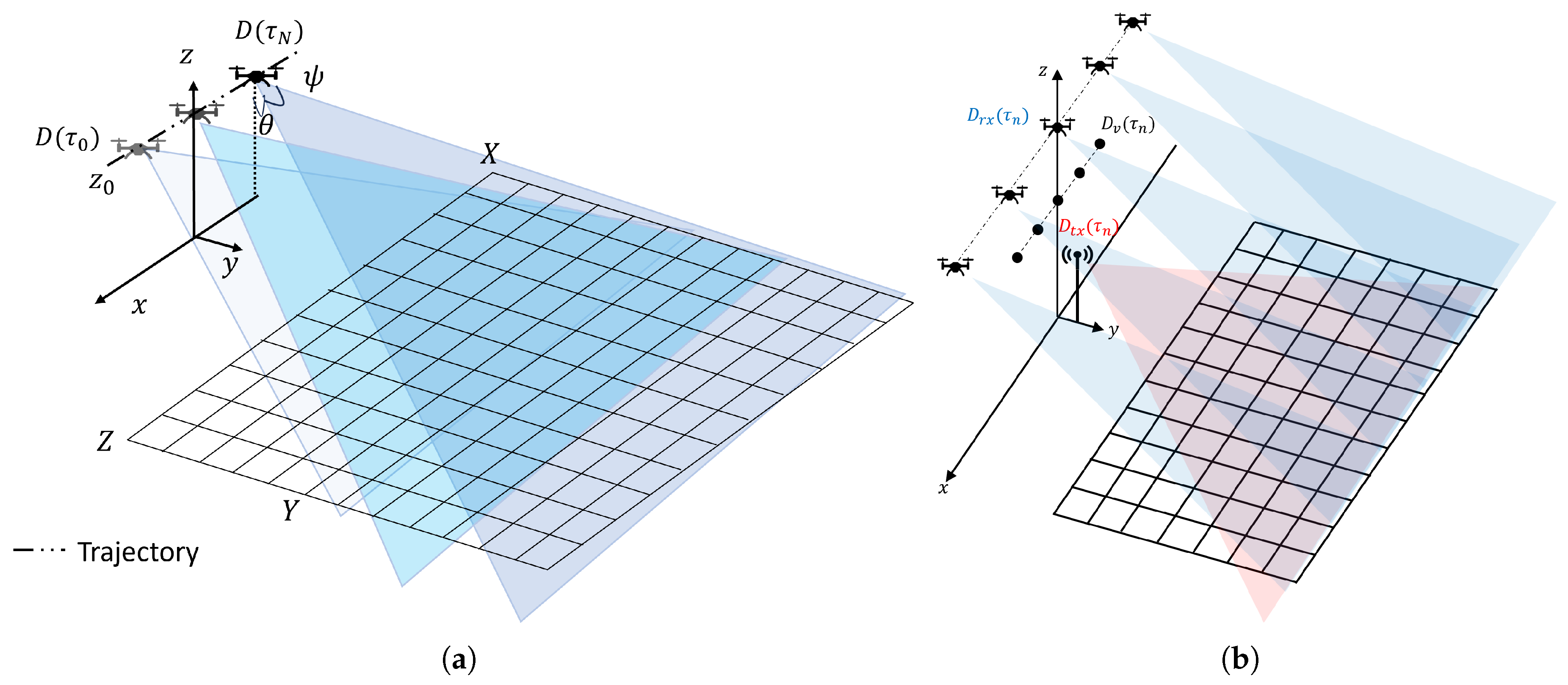
3. Flexible and Seamless Factorized Back-Projection

In this section, we will delineate the limitations of the polar reference system, and we will then formally derive a reference system with constant azimuth resolution. Next, we will explain the rationale of our focusing scheme and present the computational cost analysis upon which our work is based. Here, we will compare two focusing approaches:

• Fast Factorized Back-Projection: First, the sub-apertures are focused on a coarse grid, then the low-resolution images are merged hierarchically until the full-resolution image is obtained. This is the well-known approach developed in [20].
• Flexible & Seamless: The coarse-resolution images are merged l-wise (e.g., couple-wise) recursively until a criterion based on the computational cost is met. More precisely, at the end of each iteration step, this algorithm chooses to proceed further into the hierarchical merging or to merge all the images left into the Cartesian reference system. This approach represents our contribution described in this article.

Finally, some technical details regarding the algorithm implementation are provided.

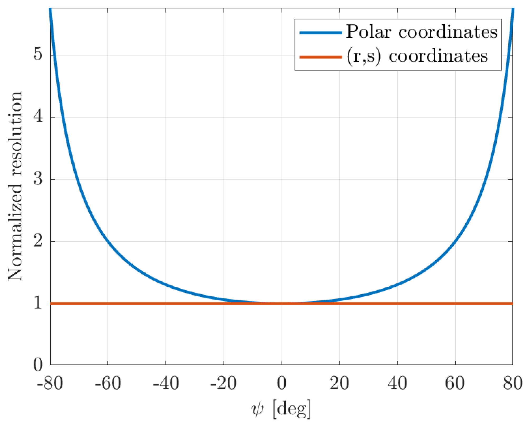
3.1. The (r,s) Reference System

In this subsection, we will analyze the Cartesian and polar reference system spectral descriptors. At the same time, we will derive a reference system with constant azimuth resolution. The Cartesian reference system resolution is expected to vary with the distance. That means, the closer the target, the finer the resolution, and the further the target, the coarser the resolution. In polar coordinates, the resolution is expected to be angular varying. Indeed, given the squint angle $\psi$, the resolution varies according to [25] as follows:

$${\rho }_{\psi }={\displaystyle \frac{\lambda }{2Acos\left(\psi \right)}}$$

(4)

In Equation (4), the angular resolution for the mono-static case is reported, where $\lambda$ is the transmitted signal wavelength, A is the considered synthetic aperture, and $\psi$ is the squint angle. Figure 1 shows how the angular resolution is not constant for varying squint angles. For example, the resolution broadens by a factor of 2 at 60 degrees. This implies that, for highly squinted targets, a less fine sampling in the angular domain is sufficient to avoid aliasing. In other words, for a high squint angle, we can allow the sampling of the polar grid to be coarser, thus reaching a lower number of samples in the back-projection grid.

A slight modification of the polar reference system, previously proposed in [30] for the forward-looking configuration (i.e., with the radar pointing in the direction of motion), is now proposed for the mono-static scenario in a side-looking configuration. Starting from the phase of the received and range-compressed signal in Equation (1),

$$\psi =-2\pi f_0\overline{t}(\mathbf{p},{\tau }_n)=-{\displaystyle \frac{4\pi }{\lambda }}R(\mathbf{p},{\tau }_n)$$

(5)

where $R(\mathbf{p},{\tau }_n)$ is the distance between the radar and the target. For the sake of simplicity, we consider a 2D distance equation. In Equation (5), the $R(\mathbf{p},{\tau }_n)$ term can be written as follows:

$$R(\mathbf{p},{\tau }_n)=\sqrt{{(x_p-x\left({\tau }_n\right))}^2+{(y_p-y\left({\tau }_n\right))}^2}$$

(6)

where

• $\mathbf{D}\left({\tau }_n\right)={[x\left({\tau }_n\right),y\left({\tau }_n\right)]}^T$ represents the position of the radar along the $(x,y)$ axis at time ${\tau }_n$;
• $\mathbf{p}={[x_p,y_p]}^T$ represents the coordinates of the target.

According to the Fundamental Diffraction Tomography Theorem [31], the spectral contributes $(k_x,k_y)$ have the form of

$$\left\{\begin{array}{c}{k}_x\left({\tau }_n\right)={\displaystyle \frac{4\pi }{\lambda }}{\displaystyle \frac{\partial R(\mathbf{p},{\tau }_n)}{\partial x}}={\displaystyle \frac{4\pi }{\lambda }}cos\psi \left({\tau }_n\right)\hfill \\ k_y\left({\tau }_n\right)={\displaystyle \frac{4\pi }{\lambda }}{\displaystyle \frac{\partial R(\mathbf{p},{\tau }_n)}{\partial y}}={\displaystyle \frac{4\pi }{\lambda }}sin\psi \left({\tau }_n\right)\hfill \end{array}\right.$$

(7)

where $\psi \left({\tau }_n\right)$ is the squint angle at the slow-time position ${\tau }_n$. It becomes straightforward that this spectral representation is space variant, i.e., it depends on both the position of the radar and on the position of the target. As detailed in [32,33], wavenumbers and resolution are linked. Their relation is expressed as follows:

$${\rho }_x={\displaystyle \frac{2\pi }{\Delta k_x}}$$

(8)

where ${\rho }_x$ is the resolution along the x-direction and $\Delta k_x$ is the width of the spectral support in the wavenumber domain covered thanks to a variation of the angle along the synthetic aperture. It is trivial to see that the resolution obtained in Equation (8) is clearly space dependent, i.e., it depends both on the target and the radar positions.

The polar reference system can be derived from the Cartesian one with the following relation:

$$\left\{\begin{array}{c}x=rsin\psi \hfill \\ y=rcos\psi \hfill \end{array}\right.$$

(9)

where r is the radius and $\psi$ is the angle. Thanks to the derivative chain rule, it is possible to compute the wavenumbers $k_{\psi }$ as follows:

$$\begin{array}{c}\hfill k_{\psi }\left({\tau }_n\right)={\displaystyle \frac{4\pi }{\lambda }}\left[{\displaystyle \frac{\partial R(\mathbf{p},{\tau }_n)}{\partial x}}{\displaystyle \frac{\partial x}{\partial \psi }}+{\displaystyle \frac{\partial R(\mathbf{p},{\tau }_n)}{\partial y}}{\displaystyle \frac{\partial y}{\partial \psi }}\right]=-{\displaystyle \frac{4\pi }{\lambda }}x\left({\tau }_n\right){\displaystyle \frac{r}{R(\mathbf{p},{\tau }_n)}}cos\psi \left({\tau }_n\right)\end{array}$$

(10)

where $\psi \left({\tau }_n\right)$ is the angle between the sensor and the target at slow time ${\tau }_n$, r is the range variable, and $R({\tau }_n,\mathbf{p})$ is the distance from the platform to the point scatter $\mathbf{p}$ at slow time ${\tau }_n$. To compute Equation (10), the platform motion along the y-direction is neglected. In Equation (10), the wavenumber with respect to the range has been neglected since we are interested in the azimuth spectral contribution. Equation (10) depends on the location of both the target and the radar; therefore, this reference system spectral estimator is space variant as well. Note that, if the squint angle $\psi$ tends to be 90 degrees, the spectral contribute $k_{\psi }\left({\tau }_n\right)$ goes to zero. This phenomenon is a dual effect with the one described for the resolution since the azimuth resolution can be computed as the inverse of the wavenumber bandwidth. Equation (10) shows a space-variant spectral descriptor unsuitable for our purpose.

Now, we will define the desired reference system as an $(r,s)$ reference system. Since one variable is the range, and the other is s, a transformation of $\psi$ is defined in the polar coordinates such that its spectral descriptor is space invariant. First, we will consider Equation (10), neglecting the y-direction contribute, and we will introduce a transformation of the polar coordinates as follows:

$$\begin{array}{c}\hfill k_s\left({\tau }_n\right)={\displaystyle \frac{4\pi }{\lambda }}\left[{\displaystyle \frac{\partial R(\mathbf{p},{\tau }_n)}{\partial x}}{\displaystyle \frac{\partial x}{\partial \psi }}{\displaystyle \frac{\partial \psi }{\partial \mathrm{s}}}\right]=-{\displaystyle \frac{4\pi }{\lambda }}x\left({\tau }_n\right){\displaystyle \frac{r}{R(\mathbf{p},{\tau }_n)}}cos\left(\psi \left({\tau }_n\right)\right){\displaystyle \frac{\partial \psi }{\partial \mathrm{s}}}\end{array}$$

(11)

The transformation introduced in Equation (11), ${\displaystyle \frac{\partial \psi }{\partial \mathrm{s}}}$, should compensate for the term $cos\left(\psi \right)$. Namely,

$${\displaystyle \frac{ds}{d\psi }}=cos\left(\psi \right)$$

(12)

By solving the differential equation in Equation (12), we can find the variable change we are looking for:

$$s\left(\psi \right)=sin\left(\psi \right)$$

(13)

Equation (13) states that, if we focus the SAR images in a reference system based on the sine of the squint angle, then it is possible to compute the spectral descriptor as

$$k_s\left({\tau }_n\right)={\displaystyle \frac{4\pi }{\lambda }}{\displaystyle \frac{rx\left({\tau }_n\right)}{R(\mathbf{p},{\tau }_n)}}$$

(14)

Another consideration is necessary in order to proceed further. We would like to apply one last approximation to achieve a complete space-invariant property. We will consider a validity region for our spectral estimator in order to remove the ratio $r/R$ in Equation (14). The validity region holds when the range variable r exceeds the synthetic aperture length [30,34]. Under this reference system, the spatial bandwidth can be computed by considering just the displacement of the platform, namely,

$$B={\displaystyle \frac{4\pi }{\lambda }}\Delta x={\displaystyle \frac{4\pi }{\lambda }}A$$

(15)

where $\Delta x$ is the displacement of the platform along the x-direction, and A is the total synthetic aperture length. Likewise, it is possible to compute the central wavenumber by using the midpoint of the aperture $x_0$ as follows:

$$k_{s_0}={\displaystyle \frac{4\pi }{\lambda }}{x}_0$$

(16)

The above equations can be referred to as Constant Spectrum Approximation (CSA). Moreover, by considering the spatial bandwidth (Equation (15)), we obtain the resolution in the s (i.e., the sine of the squint angle)-direction as follows:

$${\rho }_s={\displaystyle \frac{2\pi }{B}}={\displaystyle \frac{\lambda }{2A}}$$

(17)

As was to be expected, in the reference system described so far, the spatial resolution is revealed to depend only on the platform motion and not on the position of the target.

3.2. Flexible and Seamless Factorized Back-Projection

The procedure for our processor operates as follows: Initially, a focus area in Cartesian coordinates is selected. Once the desired azimuth resolution is established, the sampling requirements of the grid are determined. Next, a trajectory to be focused is chosen and divided into sub-apertures. These sub-apertures are then processed at an s-coarse resolution in the $(r,s)$ reference system. For the mono-static case, the resulting images are associated with the central position of each sub-aperture phase center, whereas, for the bi-static case, they are associated with the central position of the VPC sub-apertures.

Subsequently, two strategies are evaluated. The first approach involves merging all coarse-resolution images into a Cartesian reference system centered at the trajectory midpoint, implementing the fast back-projection method [35]. The alternative approach involves conducting a single step of hierarchical merging. After each step of hierarchical merging, the same choice arises: either to proceed with a global merge or to continue with an additional hierarchical merging step. This process is repeated for every feasible hierarchical step until a full-resolution SAR image is generated. The decision to proceed further into hierarchical merging at each iteration is guided by computational cost considerations. At the conclusion of each step, the algorithm evaluates whether to continue hierarchical merging or terminate based on the anticipated computational effort. A visual representation of the decision tree is given in Figure 2.

3.3. Computational Cost Analysis

In this subsection, we will perform a detailed analysis of the computational cost for Flexible & Seamless. Here, the computational costs are considered as the number of complex operations required to perform imaging, the net of the interpolation kernel. First, we will tackle the sub-aperture focusing, and second, the fast back-projection implementation. Later, the hierarchical merging phase is analyzed, and, finally, the global Cartesian merging step.

First of all, the sub-apertures are focused in an s-coarse-resolution reference system, depending on the sub-aperture length. Let us define the initial size of the s-coarse axis as $N_t^{\left(0\right)}$, and the number of samples in a sub-aperture and in the trajectory as $N_s$ and $N_{\tau }$, respectively. The computational cost required to focus all the sub-apertures with TDBP is given by the following:

$$O\left({\displaystyle \frac{N_{\tau }}{N_s}}{N}_t^{\left(0\right)}{M}_r{N}_s\right)$$

(18)

where $\left[M,N_t^{\left(0\right)}\right]$ is the dimension of the coarse-resolution grid. The cost to focus a single sub-aperture is proportional to the number of slow-time samples used to focus it and the number of pixels of the grid, leading to a cost for a single aperture of $N_t^{\left(0\right)}{M}_r{N}_s$. Moreover, this cost must be multiplied by the number of sub-apertures contained in the trajectory to be processed, i.e., by $N_{\tau }/N_s$. Note that the interpolation kernel has been neglected. Equation (19) can be further simplified as follows:

$$O\left(N_{\tau }{N}_t^{\left(0\right)}{M}_r{N}_s\right)$$

(19)

Now, two paths are ahead. Merging all the sub-apertures in a single step will lead to a computational cost of

$$O\left({\displaystyle \frac{N_{\tau }}{N_s}}{N}_x{N}_y\right)$$

(20)

where $\left[N_x,N_y\right]$ is the size of the Cartesian image size. A single interpolation costs roughly $N_x{N}_y$ and must be performed once for every sub-aperture; thus, the cost scales by $N_{\tau }/N_s$. Moving further into the hierarchical merging section of the computational cost diagram in Figure 2, the size of the s-axis becomes l times wider at each iteration step since the processed aperture enlarges by a factor l. On the contrary, the number of images to be merged is reduced by a factor l for each step. The computational costs related to this implementation are as follows:

$$O\left(\sum _{k=0}^K{l}^{K-k}{N}_t^{(k+1)}{M}_r\right)$$

(21)

where k is the hierarchical step of the procedure, $K=lo{g}_l(N_{\tau }/N_s)$ is the maximum number of hierarchical steps performable, the factor $l^{K-k}$ represents the number of images left at the iteration step k, and $\left[N_t^{\left(k\right)},M_r\right]$ is the image size at step k. By using Equations (19) and (21), it is possible to compute the computational burden for Fast Factorized Back-Projection as follows:

$$O\left(N_{\tau }{N}_t^{\left(0\right)}{M}_r{N}_s+\sum _{k=0}^K{l}^{K-k}{N}_t^{(k+1)}{M}_r\right)$$

(22)

Equation (22) is the computed net of the interpolation kernel. The cost to merge all the $(r,s)$ images left at step k into the Cartesian domain is provided by the following:

$$O\left(l^{K-k}{N}_x{N}_y\right)$$

(23)

where the couple $\left[N_x,N_y\right]$ is the $(x,y)$ image size. The advantage of this algorithm lies in the hierarchical merging phase structure. Since the number of images shrinks by a factor l at each iteration step, merging the images in a global Cartesian reference system becomes less and less expensive. On the contrary, the hierarchical merging cost remains almost constant since the number of images shrinks by a factor l, but the number of samples in the s-axis scales linearly with l. Thus, at some point in the iteration phase, the number of complex operations required for the global Cartesian merging will be less computationally expensive than performing a factorization step. Therefore, Flexible & Seamless is granted to reach a full-resolution SAR image with the lowest operational cost possible. In light of the above analysis, the entire computational cost for the Flexible & Seamless implementation is given by Equations (19), (21) and (23) as follows:

$$O\left(N_{\tau }{N}_t^{\left(0\right)}{M}_r+\sum _{k=0}^{\tilde{k}}{l}^{K-k}{N}_t^{(k+1)}{M}_r+l^{K-\tilde{k}}{N}_x{N}_y\right)$$

(24)

where the index $\tilde{k}$ is the hierarchical step providing the minimum computational cost.

3.4. Algorithm Implementation

Some technicalities in the implementation are covered in this section. To reduce the computational costs, during the sub-aperture focusing procedure, the s-variable axis has been limited to a value $s_{max}$, depending on the resolution achievable:

$$s_{max}=sin\left({\displaystyle \frac{\lambda }{2{\rho }_x}}\right)$$

(25)

where ${\rho }_x$ is the desired resolution. Then, during the hierarchical merging, the $s_{max}$ value is stretched linearly at each step up to its maximum ($s_{max}=1$) to preserve the information about the scene. Another detail regards the sampling in the s-variable domain. While focusing the sub-apertures, the s-variable sampling is related to the sub-aperture length. In the second phase of the algorithm, the sampling bottleneck is given by the minimum between the available aperture length and the aperture required to obtain ${\rho }_x$. These two passages reduce the computational costs and must be accounted for in the computation of $N_t^{\left(k\right)}$. Moreover, a problem with the sub-aperture merging arises. Two successive apertures can be at different altitudes, using different off-nadir angles. This must be accounted for in the merging procedure as well. The set of equations we are proposing is the following:

$$\left\{\begin{array}{c}s={\displaystyle \frac{x-D_x}{r}}=sin\left(\psi \right)\hfill \\ y-D_y=rcos\left(\psi \right)sin\left(\theta \right)\hfill \\ z-D_z=r\sqrt{1-s^2}cos\left(\theta \right)\hfill \end{array}\right.$$

(26)

where the couple $(r,s)$ represents the $(r,s)$ reference system, the triple $(x,y,z)$ represents the Cartesian reference system, $\mathbf{D}=(D_x,D_y,D_z)$ represents the UAV space coordinates, $\theta$ is the off-nadir, and $\psi$ is the squint angle. The equations in Equation (26) allow us to include the elevation angle $\theta$ in the definition of the reference system $(r,s)$. The above-defined equations allow us to map the Cartesian reference system in the $(r,s)$ reference system, namely, to go from $(x,y,z)$ to $(r,s)$ and back. Moreover, given two different $(r,s)$ images, $I(r,s,{\tau }_j)$ and $I(r,s,{\tau }_k)$, focused from two different sub-aperture centers of the UAV trajectory, $\mathbf{D}\left({\tau }_j\right)$ and $\mathbf{D}\left({\tau }_k\right)$, it is possible to map them as if they where focused from a third phase center position $\mathbf{D}\left({\tau }_t\right)$. First, $I(r,s,{\tau }_j)$ and $I(r,s,{\tau }_k)$ are mapped into the common $(x,y,z)$ reference system. Then, from $(x,y,z)$, the two are mapped back into the $(r,s)$ by pouring the phase center position $\mathbf{D}\left({\tau }_t\right)$ into Equation (26). This procedure is handy in the hierarchical implementation of the Flexible & Seamless algorithm.

4. Numerical Analysis

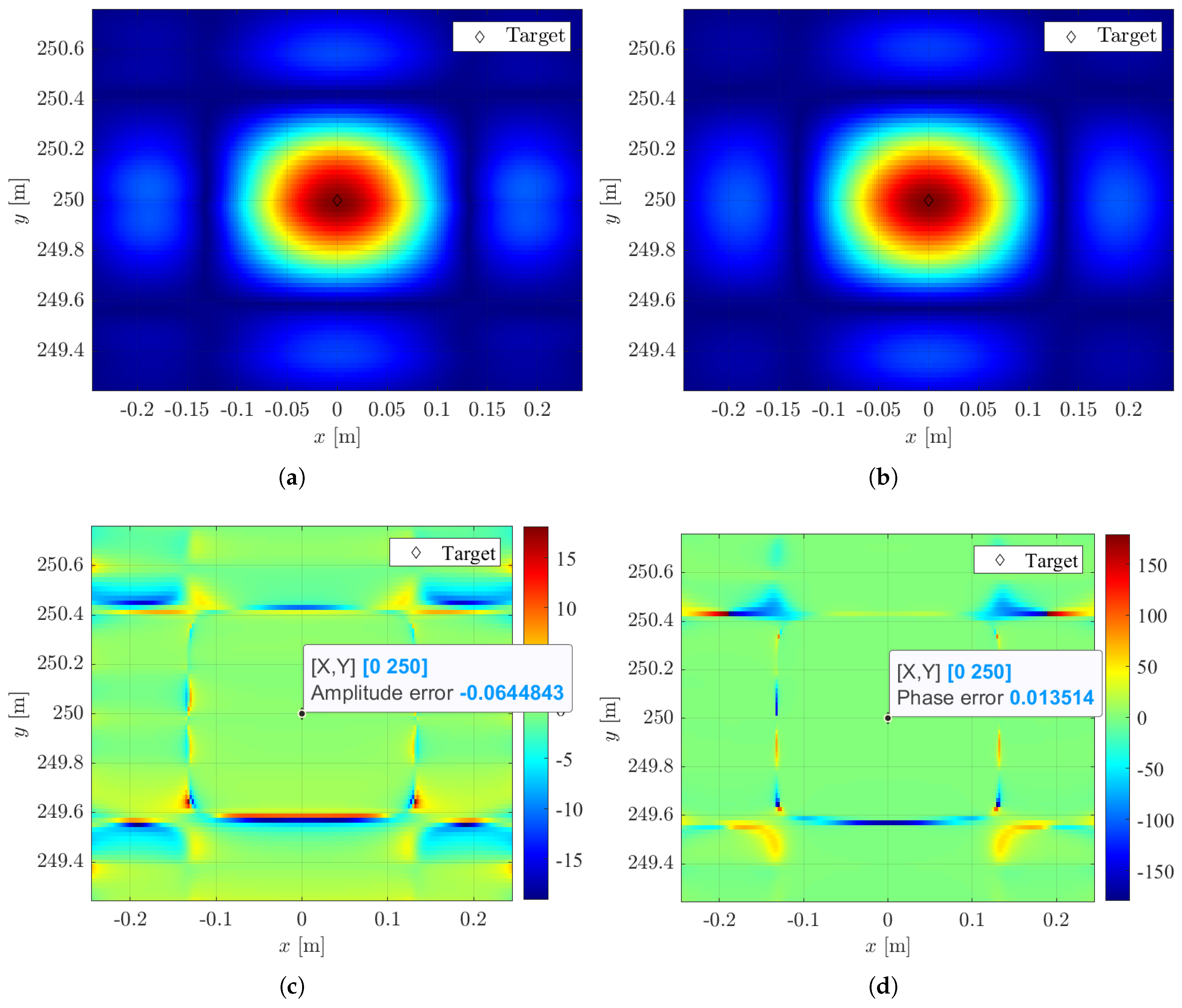
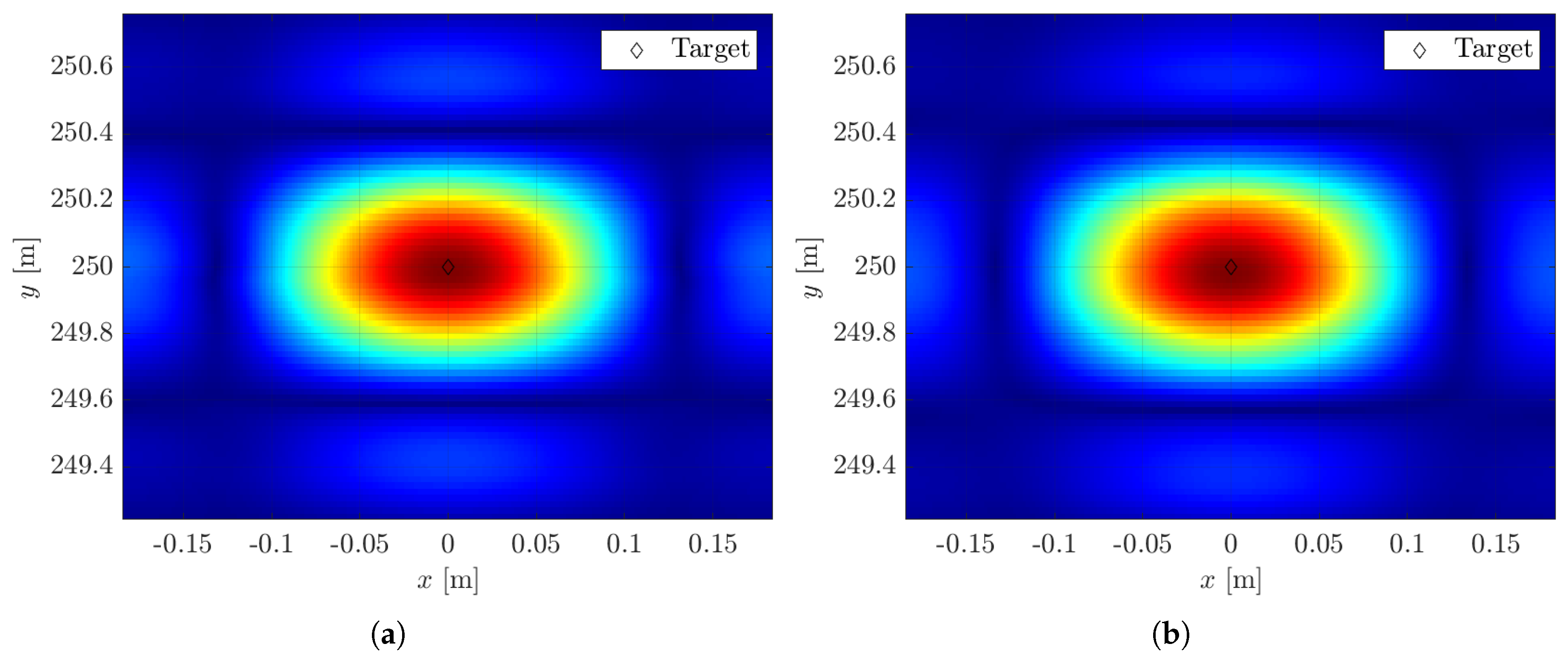
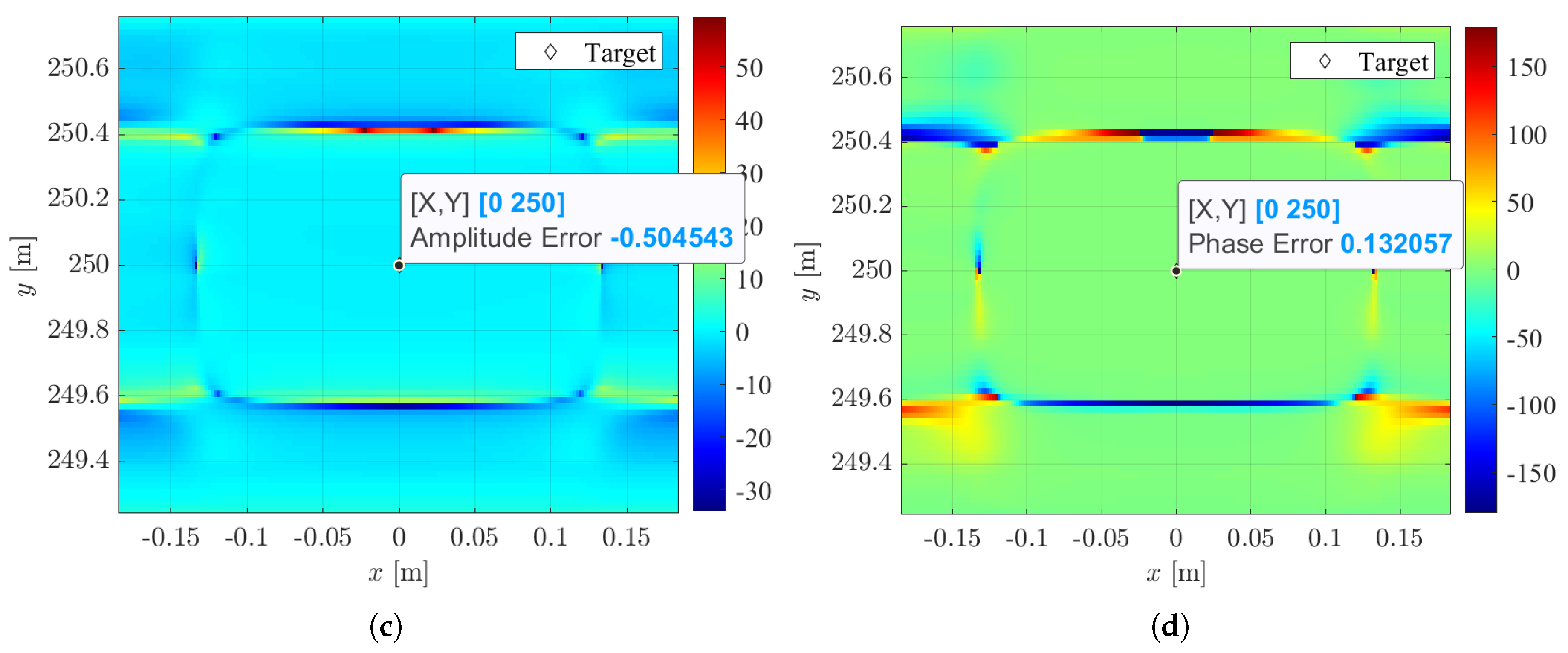
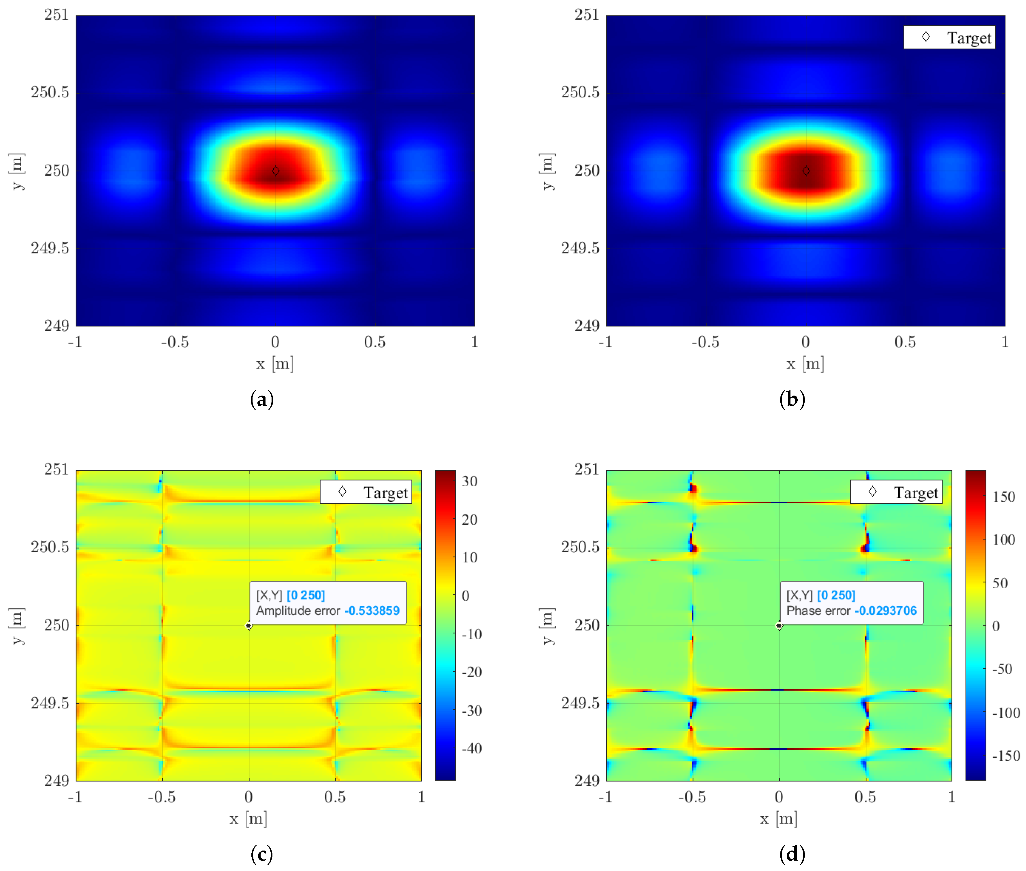
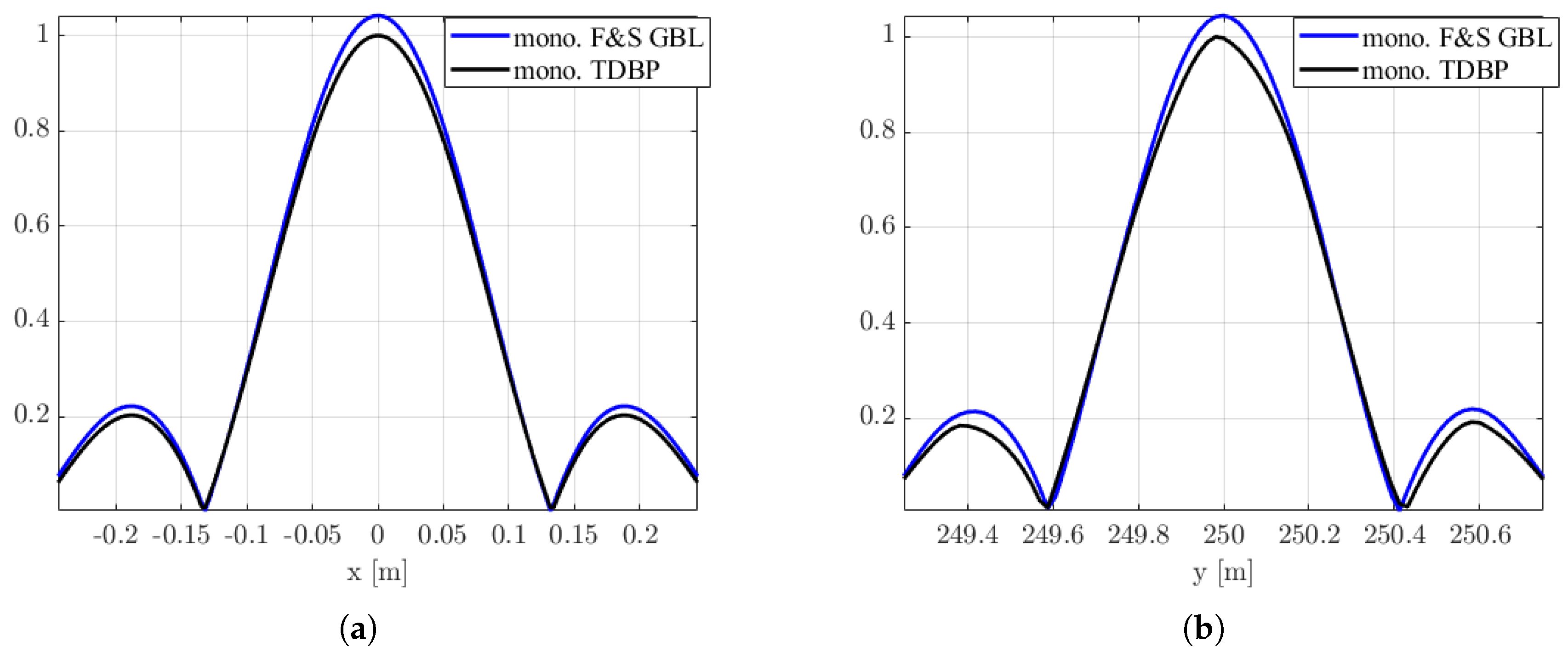
In this section, we propose a comparative analysis of the two algorithms. Here, two operative scenarios are defined for both mono- and bi-static implementation. Then, the computational costs for both configurations are proposed for each scenario. Finally, a comparison between the two algorithms is presented, considering a large-scale scenario. We simulated an SAR system operating in the X-band at $9.45$ GHz with a transmitted signal bandwidth of 400 MHz for both mono-static and bi-static cases. The area under consideration for the focusing algorithm spans 120 m in azimuth and 500 m in slant range. The simulated parameters are summed up in

Table 1. UAV-SAR system parameters.

Parameter	Symbol	Value
Central frequency	$f_0$	9.45 GHz
Bandwidth	B	400 MHz
Lambda	$\lambda$	0.0317 m
Range resolution	${\rho }_r$	0.4 m
Area dimensions	$(x,y)$	(120 m, 500 m)

.

4.1. UAV Scenarios

The scenarios under consideration consider both mono-static and bi-static SAR systems. The former scenario is referred to as a ground-based-like (GBL) UAV-borne SAR scenario. The GBL scenario consists of a short trajectory and a wide area to be illuminated by the SAR experiment. In the mono-static case, it consists of a single-channel radar mounted on a UAV, traveling for a short trajectory with respect to the enlightened area. The bi-static case uses a still transmitter and a moving receiver. The two configurations of this scenario are shown in Figure 3. In this case, the azimuth resolution is space varying, which means that it is finer for the near range and wider in the far range, following the azimuth resolution law [36]

$${\rho }_{az}={\displaystyle \frac{\lambda }{cos(\beta /2)}}{(A_{tx}/R_{tx}+A_{rx}/R_{rx})}^{-1}$$

(27)

where $\lambda$ is the transmitted signal wavelength, and $\beta$ is the bi-static angle, namely, the angle subtended between the transmitter, target, and receiver. $A_{tx}$ and $A_{rx}$ are the apertures spanned by the transmitter and the receiver, respectively, while $R_{tx}$ and $R_{rx}$ are the one-way distances between the target and the tx antenna and the rx antenna, respectively. Equation (27) is proposed for the bi-static radar configuration. Note that, when the transmitter and the receiver positions coincide, the bi-static angle $\beta$ is 0, and the resolution ${\rho }_{az}$ converges to the well-known mono-static azimuth resolution formula $\lambda /\left(2A\right)R$ [25], where R is the one-way distance from the platform to the scene.

The second scenario is a proper stripmap scenario. The mono-static case is deployed similarly to the GBL UAV-borne SAR scenario but with a longer trajectory covering the entire scene, to obtain a constant azimuth resolution. The bi-static case comprises two UAVs flying along the same direction with a fixed bi-static baseline, i.e., the distance between the transmitter and the receiver. The proposed stripmap scenario is shown in Figure 4.

4.2. Ground-Based-like Scenario

The GBL scenario is characterized by a short trajectory with respect to the enlightened area. In the mono-static case, the radar’s aperture spans the entire trajectory of about 15 m, flying at an altitude of 30 m. In the bi-static case, only the receiver is moving, while the transmitter is still. In the latter case, the trajectory traveled by the platform is about 15 m. The receiver is flying at 30 m, while the transmitter is at a fixed height of 10 m. The two geometries are reported in

Table 2. GBL scenario geometry.

Parameter	Mono-Static	Bi-Static
Tx trajectory	15 m	0 m
Rx trajectory	15 m	15 m
Tx altitude	30 m	30 m
Rx altitude	30 m	30 m

. Note that, in Table 2, the positions of the transmitter and the receiver in the mono-static case coincide.

In this scenario, we settle for a space-varying resolution according to Equation (27). Due to this, the Cartesian images are highly sampled in order to meet the Nyquist criteria in near range. Here, Flexible & Seamless achieves the same performances as the Fast Factorized Back-Projection. This is due to the almost polar geometry of the scenario. The computational cost curves are reported in Figure 5. Figure 5a reports the computational curves for the mono-static case, while Figure 5b reports the curves for the bi-static case.

4.3. Stripmap Scenario

The proposed scenario is a stripmap scenario with a constant azimuth resolution to be tuned as a system parameter. For the mono-static case, the considered aperture is about 250 m. In the bistatic case, the two UAVs are considered to fly with a fixed bi-static baseline of about 40 m for a 250 m trajectory. In both the mono-static and bi-static cases, the UAVs are supposed to fly at an altitude of 30 m. These scenario parameters are summarized in

Table 3. Stripmap scenario geometry.

Parameter	Mono-Static	Bi-Static
Tx trajectory	250 m	250 m
Rx trajectory	250 m	250 m
Tx altitude	30 m	30 m
Rx altitude	30 m	30 m
Bi-static baseline	˜	40 m
Azimuth resolution	0.25 m	0.5 m

. Note that, in Table 3, the positions of the transmitter and the receiver in the mono-static case coincide. In this case, since the resolution is fixed for the entire scene, both in the near range and in the far range, the Cartesian grid has a lower number of samples than the full $(r,s)$ image. Flexible & Seamless is expected to interrupt the hierarchical merging in the factorization and to merge all the images remaining at that moment in a single common Cartesian reference system. During the hierarchical merging operation, the hierarchical merging will be more computationally demanding than merging all the images into a common reference system. Thus, in this way, our algorithm will be faster than standard FFBP.

The computational cost curves are reported in Figure 6. Figure 6a reports the computational curves for the mono-static case, while Figure 6b reports the curves for the bi-static case. In both the cases, our algorithm gains a computational cost advantage of about $43\%$ compared with the FFBP implementation.

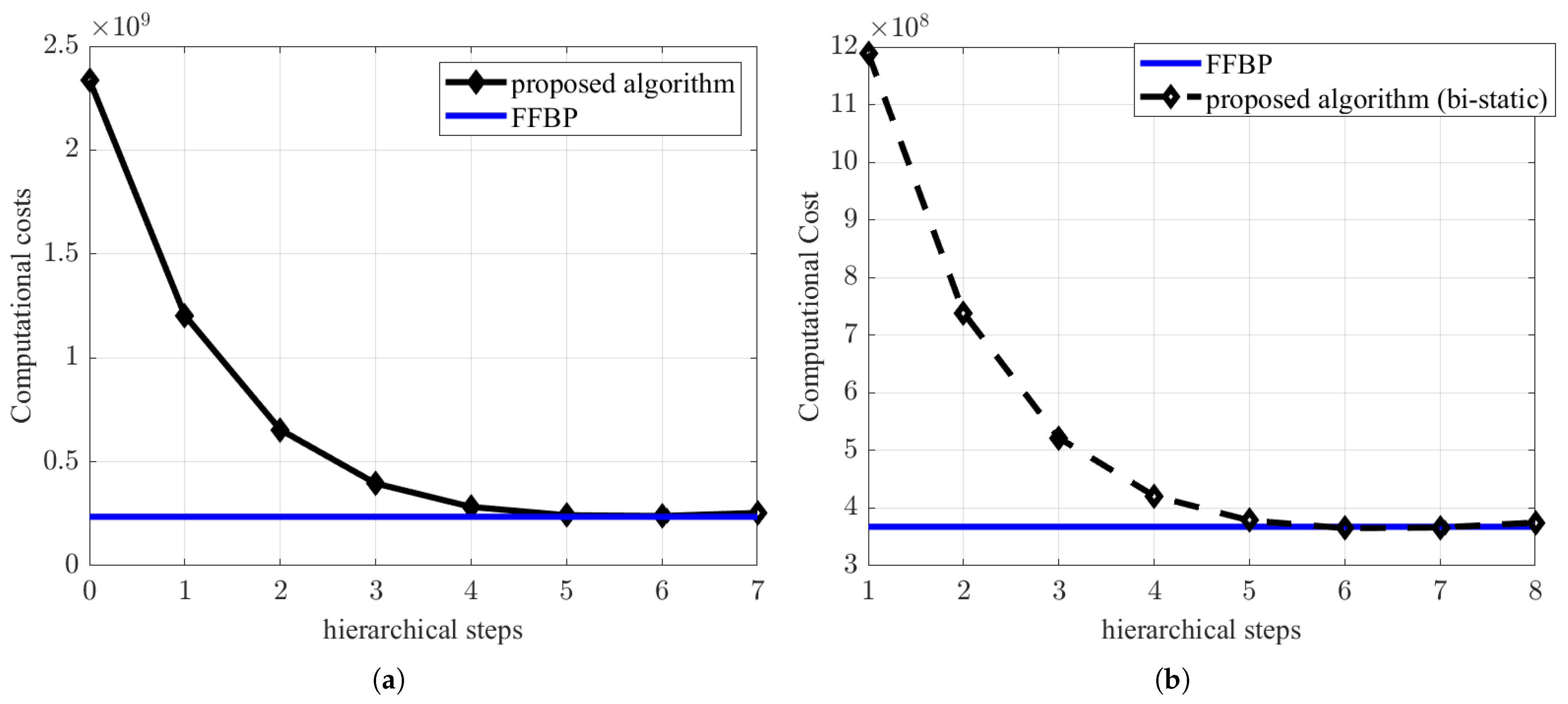
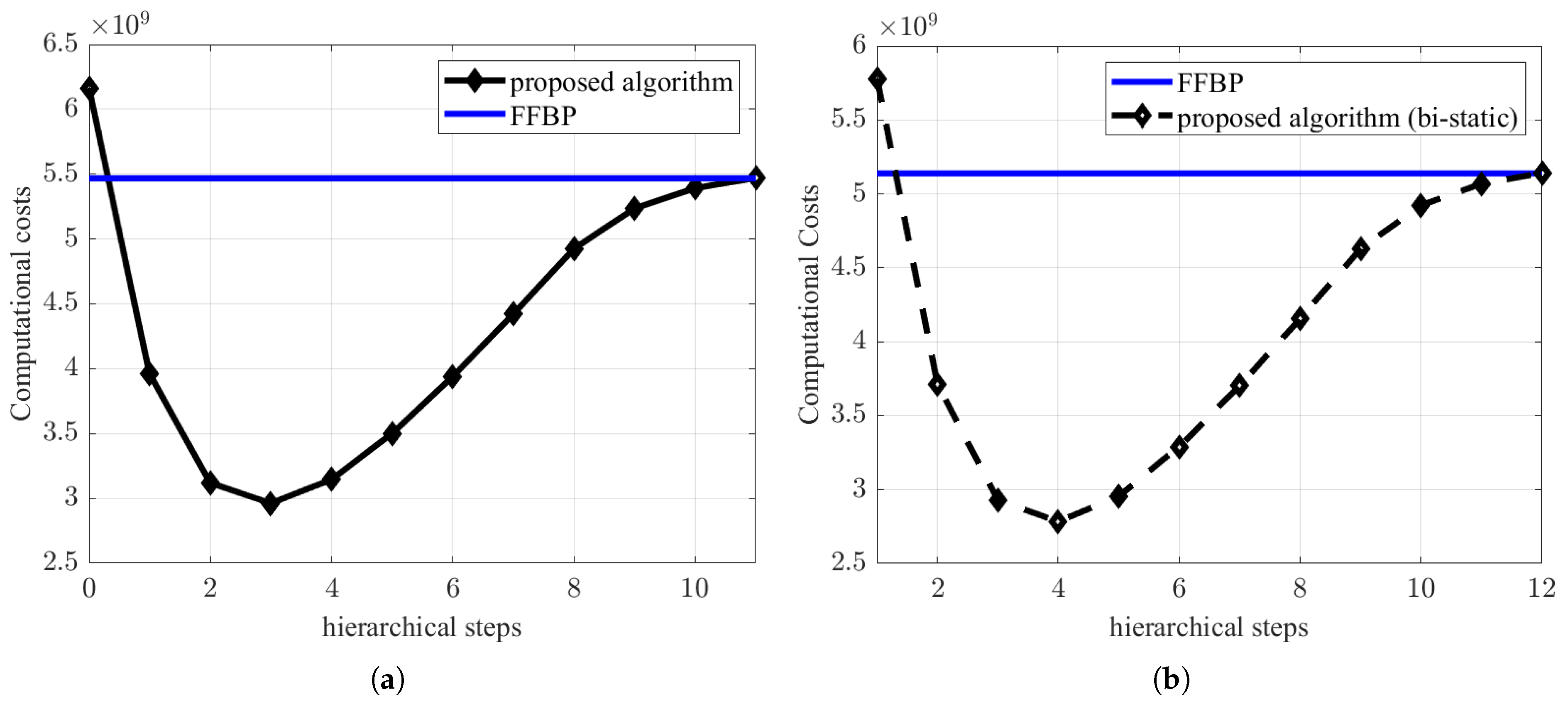
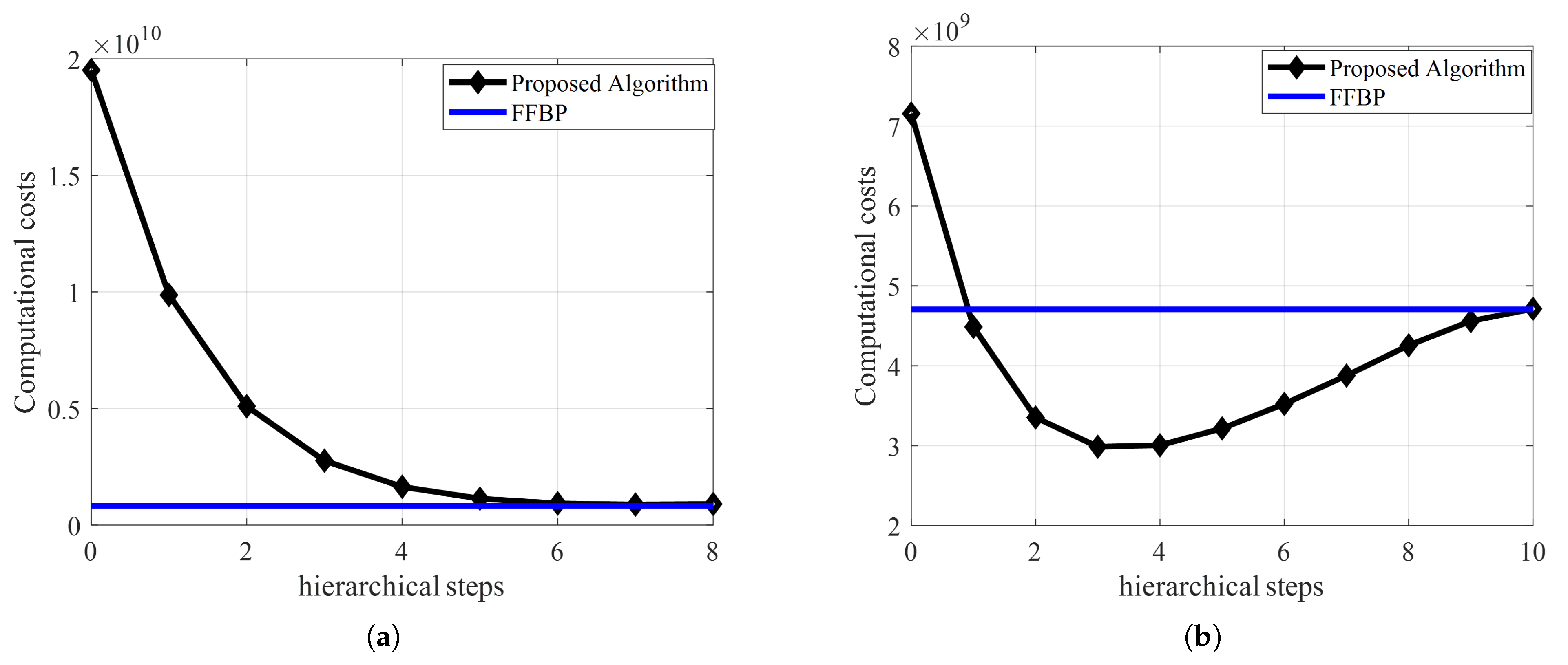
4.4. A Computational Cost Comparison Between Large-Scale FFBP and Flexible & Seamless

In this subsection, we propose a comparison between a large-scale implementation of FFBP and of our algorithm. The point of this is to show that, even in a large-scale scenario, with a highly variational incident angle in the SAR swath, Flexible & Seamless is a better-performing algorithm. Let us define a scenario belonging to the stripmap scenario. We will consider a scenario with an azimuth width of 4 km and a range length of 2 km, a desired azimuth resolution of $0.2$ m, a trajectory length of about 4 km, and a flying height of 30 m. These comparison parameters are summarized in

Table 4. Computational cost comparison parameters.

Parameter	Symbol	Value
Area dimensions	$(x,y)$	(4 km, 2 km)
Range resolution	${\rho }_r$	0.4 m
Azimuth resolution	${\rho }_x$	0.2 m
Trajectory length	˜	4 km
Flying height	$z_h$	30 m

.

Focusing such a scenario using TDBP will take a number of complex operations of about $2.2\times {10}^{14}$. Now, we will compare the computational costs to focus such a scenario using an overlap-and-add (OaA) approach. The OaA approach consists of cropping the trajectory into segments that are used to focus a slice of the scenario. The obtained image overlaps the two adjacent images. We have considered a $25\%$ overlap between adjacent segments. Then, the obtained images are summed together to achieve a constant-resolution image of the scenario. Here, the trajectory is divided into segments of about 150 m each. Each segment is used to focus a slice of the scenario of approximately 370 m. The comparison is proposed in terms of complex operations to be performed to focus the image. FFBP and our algorithms have been used as focusing kernels to focus the segments of the trajectory. FFBP takes $4\times {10}^{11}$ complex operations to focus the scenario, while our algorithm needs $2.5\times {10}^{11}$ complex operations. Thus, the Flexible & Seamless implementation is more efficient also in a large-scale scenario.

5. Numerical Simulation

In this section, we propose a numerical evaluation of our algorithm. We will consider the algorithm’s accuracy in both phase and amplitude using Time-Domain Back-Projection as a benchmark for our evaluation. All the scenarios in Section 4 are proposed. We want to remark that, for these point target simulations, perfectly straight trajectories sampled at $\lambda /4$ are used, for the mono-static cases and for the bi-static stripmap scenario. In the bi-static GBL scenario, the transmitter is still and the receiver is moving on a straight line sampled at $\lambda /4$ as well. The phase error has been computed by performing the pointwise conjugate product between the Flexible & Seamless image and the complex conjugate of the benchmark image. This results in a phase difference between the Flexible & Seamless image and the TDBP one. The amplitude error is computed by evaluating in dB the ratio between the Flexible & Seamless image and the benchmark one. Additionally, a comparison between the Flexible & Seamless impulse responses in range and in azimuth is presented. These are normalized with respect to the peak of the TDBP image for both the Flexible & Seamless image and the TDBP image. The system impulse responses for the mono-static GBL case are reported in Figure 7a,b for the benchmark and our algorithm, respectively. Also, the amplitude error and the phase error are reported, respectively, in Figure 7c,d for the mono-static GBL case. In Figure 7c, the error expressed in dB in the point scatter location is about $0.06$ dB. In Figure 7d, the phase error between the benchmark and our algorithm result is about $0.01$ degrees. The system impulse responses for the bi-static GBL case are reported in Figure 8a,b, for the benchmark and our algorithm, respectively.

Also, the amplitude error and the phase error are reported, respectively, in Figure 8c,d for the bi-static case. In Figure 8c, the error expressed in dB, in the point scatter location is about $0.5$ dB, while, in Figure 8d the phase error between the benchmark and our algorithm result is about $0.1$ degrees.

The system impulse responses for the mono-static stripmap case are reported in Figure 9a,b for the benchmark and our algorithm, respectively. Also, the amplitude error and the phase error are reported, respectively, in Figure 9c,d. In Figure 9c, the error expressed in dB in the point scatter location is about $0.2$ dB. In Figure 9d, the phase error between the benchmark and our algorithm result is about $0.003$ degrees.

The system impulse responses for the bi-static stripmap case are reported in Figure 10a,b for the benchmark and our algorithm, respectively. Also, the amplitude error and the phase error are reported, respectively, in Figure 10c,d for the bi-static case. In Figure 10c, the error expressed in dB in the point scatter location is about $-0.5$ dB, while, in Figure 8d, the phase error between the benchmark and our algorithm result is about $-0.02$ degrees. The azimuth and range profiles of the point scatterer in the GBL scenario simulation are reported in Figure 11. Figure 11a,b are relative to the mono-static azimuth and range profile, respectively, and Figure 11c,d to the bi-static GBL scenario. In Figure 11, the profiles have been normalized with respect to the TDBP image peak.

The azimuth and range profiles of the point scatterer in the stripmap scenario simulation are reported in Figure 12. Figure 12a,b are relative to the mono-static azimuth and range profile, respectively, and Figure 12c,d to the bi-static GBL scenario. In Figure 12, the profiles have been normalized with respect to the TDBP image peak.

6. Real Data

The algorithm has been validated through some real data acquired with an X-band radar in a mono-static configuration. The experiment took place in a dedicated area next to Milan. Our UAV setup can be found in Figure 13a. It consisted of an off-the-shelf UAV using as a payload a radar developed by Aresys.sr^®. The illuminated area was about $(120,500)$ m, with a trajectory of 120 m, at an altitude of 30 m. The optical image of interest can be found in Figure 13b. The transmitted signal carrier frequency was $9.45$ GHz using a bandwidth of 400 MHz, thus giving a range resolution of about $0.4$ m. Both the mono-static GBL and the mono-static stripmap scenarios were considered. The experimental parameters are reported in

Table 5. Real data experiment parameters.

Parameters	GBL	Stripmap
Carrier frequency	$9.4$5 GHz	$9.45$ GHz
Bandwidth	400 MHz	400 MHz
Aperture	32 m	120 m
Altitude	30 m	30 m
Area	$(120,500)$ m	$(120,500)$ m
Azimuth resolution	˜	$0.08$ m
Range resolution	$0.4$ m	$0.4$ m

. The data were autofocused using the procedure outlined in [37,38].

The experiment focused both in stripmap and in GBL configuration. While the GBL configuration used a portion of the trajectory of about 32 m, the stripmap configuration considered the entire trajectory. In the GBL scenario, the azimuth resolution was space variant, while, in the stripmap scenario, the resolution was constant at a fixed value of $0.08$ m. Fist, we propose the GBL UAV-borne SAR scenario. In Figure 14a, the computational costs are proposed. Figure 14a shows that the GBL scenario has the same performances as the FFBP, as expected.

The focused image in the mono-static GBL configuration is proposed in Figure 15a. Then, the stripmap scenario is proposed. In Figure 14b, the computational cost curves are proposed. Here, due to the long trajectory considered and the constant resolution in azimuth, Flexible & Seamless outperforms the FFBP algorithm. In Figure 14b, it is shown that the optimal hierarchical steps required for the minimum computational cost are 3. In this case, the computational cost advantage is $37.5\%$. The focused image for our scenario is reported in Figure 15b. Both the GBL scenario and the stripmap scenario show consistency with the optical image of the proposed scene.

7. Conclusions

This paper introduces a novel factorized processor termed Flexible & Seamless Factorized Back-Projection, designed to focus UAV-borne SAR images in both mono-static and bi-static configurations. Two operational scenarios for UAV-borne SAR experiments are defined: the ground-based-like (GBL) scenario and the stripmap scenario. The GBL scenario features a short platform trajectory, resulting in space-varying azimuth resolution, while the stripmap scenario involves a longer trajectory with constant azimuth resolution, characteristic of conventional stripmap SAR. A customized reference system was analyzed to optimize the implementation of Time-Domain Back-Projection (TDBP). A computational cost analysis was conducted, providing an assessment of the algorithm’s computational complexity. This analysis serves as a metric for selecting the most efficient algorithm for SAR imaging in specific scenarios. In the stripmap scenario, Flexible & Seamless surpassed FFBP in computational efficiency, while, in the GBL scenario, it matched the performance of FFBP. Numerical simulations demonstrated the proposed algorithm’s accuracy in both amplitude and phase, using TDBP as the benchmark for evaluation. Furthermore, the algorithm was validated through a real data experiment conducted in the X-band near Milan, confirming its consistency with the corresponding optical scenario.

References

1. Petritoli, E.; Leccese, F.; Ciani, L. Reliability assessment of UAV systems. In Proceedings of the 2017 IEEE International Workshop on Metrology for AeroSpace (MetroAeroSpace), Padua, Italy, 21–23 June 2017; pp. 266–270. [Google Scholar]
2. Meng, K.; Wu, Q.; Xu, J.; Chen, W.; Feng, Z.; Schober, R.; Swindlehurst, A.L. UAV-enabled integrated sensing and communication: Opportunities and challenges. IEEE Wirel. Commun. 2023, 31, 97–104. [Google Scholar] [CrossRef]
3. Zeng, Y.; Zhang, R.; Lim, T.J. Wireless communications with unmanned aerial vehicles: Opportunities and challenges. IEEE Commun. Mag. 2016, 54, 36–42. [Google Scholar] [CrossRef]
4. Schreiber, E.; Heinzel, A.; Peichl, M.; Engel, M.; Wiesbeck, W. Advanced buried object detection by multichannel, UAV/drone carried synthetic aperture radar. In Proceedings of the 2019 13th European Conference on Antennas and Propagation (EuCAP), Krakow, Poland, 31 March–5 April 2019; pp. 1–5. [Google Scholar]
5. Romero, I.; Walter, T.; Mariager, S. Performance Analysis and Simulation of a Continious Wave Metal Detector for UAV Applications. In Proceedings of the IGARSS 2022—2022 IEEE International Geoscience and Remote Sensing Symposium, Kuala Lumpur, Malaysia, 17–22 July 2022; pp. 7222–7225. [Google Scholar]
6. Angelliaume, S.; Castet, N.; Dupuis, X. SAR-Light: The new ONERA SAR sensor on-board UAV. IET Conf. Proc. 2022, 17, 66–70. [Google Scholar] [CrossRef]
7. Lort, M.; Aguasca, A.; Lopez-Martinez, C.; Marín, T.M. Initial evaluation of SAR capabilities in UAV multicopter platforms. IEEE J. Sel. Top. Appl. Earth Obs. Remote Sens. 2017, 11, 127–140. [Google Scholar] [CrossRef]
8. Brigui, F.; Angelliaume, S.; Castet, N.; Dupuis, X.; Martineau, P. Sar-light-first sar images from the new onera sar sensor on uav platform. In Proceedings of the IGARSS 2022—2022 IEEE International Geoscience and Remote Sensing Symposium, Kuala Lumpur, Malaysia, 17–22 July 2022; pp. 7721–7724. [Google Scholar]
9. Linsalata, F.; Albanese, A.; Sciancalepore, V.; Roveda, F.; Magarini, M.; Costa-Perez, X. OTFS-superimposed PRACH-aided localization for UAV safety applications. In Proceedings of the 2021 IEEE Global Communications Conference (GLOBECOM), Madrid, Spain, 7–11 December 2021; pp. 1–6. [Google Scholar]
10. Manzoni, M.; Moro, S.; Linsalata, F.; Polisano, M.G.; Monti-Guarnieri, A.V.; Tebaldini, S. Evaluation of UAV-Based ISAC SAR Imaging: Methods and Performances. In Proceedings of the 2024 IEEE Radar Conference (RadarConf24), Denver, CO, USA, 6–10 May 2024; pp. 1–6. [Google Scholar] [CrossRef]
11. Denbina, M.; Towfic, Z.J.; Thill, M.; Bue, B.; Kasraee, N.; Peacock, A.; Lou, Y. Flood mapping using UAVSAR and convolutional neural networks. In Proceedings of the IGARSS 2020—2020 IEEE International Geoscience and Remote Sensing Symposium, Waikoloa, HI, USA, 26 September–2 October 2020; pp. 3247–3250. [Google Scholar]
12. Cafforio, C.; Prati, C.; Rocca, F. SAR data focusing using seismic migration techniques. IEEE Trans. Aerosp. Electron. Syst. 1991, 27, 194–207. [Google Scholar] [CrossRef]
13. Bamler, R. A comparison of range-Doppler and wavenumber domain SAR focusing algorithms. IEEE Trans. Geosci. Remote Sens. 1992, 30, 706–713. [Google Scholar] [CrossRef]
14. Frey, O.; Meier, E.H.; Nüesch, D.R. Processing SAR data of rugged terrain by time-domain back-projection. In Proceedings of the SAR Image Analysis, Modeling, and Techniques VII, Bruges, Belgium, 19–22 September 2005; Volume 5980, pp. 71–79. [Google Scholar]
15. Frey, O.; Magnard, C.; Rüegg, M.; Meier, E. Non-linear SAR data processing by time-domain back-projection. In Proceedings of the 7th European Conference on Synthetic Aperture Radar, Friedrichshafen, Germany, 2–5 June 2008; pp. 1–4. [Google Scholar]
16. Frey, O.; Magnard, C.; Ruegg, M.; Meier, E. Focusing of airborne synthetic aperture radar data from highly nonlinear flight tracks. IEEE Trans. Geosci. Remote Sens. 2009, 47, 1844–1858. [Google Scholar] [CrossRef]
17. Frey, O.; Werner, C.L.; Wegmuller, U. GPU-based parallelized time-domain back-projection processing for agile SAR platforms. In Proceedings of the 2014 IEEE Geoscience and Remote Sensing Symposium, Quebec City, QC, Canada, 13–18 July 2014; pp. 1132–1135. [Google Scholar]
18. Frey, O.; Werner, C.L.; Coscione, R. Car-borne and UAV-borne mobile mapping of surface displacements with a compact repeat-pass interferometric SAR system at L-band. In Proceedings of the IGARSS 2019-2019 IEEE International Geoscience and Remote Sensing Symposium, Yokohama, Japan, 8 July–2 August 2019; pp. 274–277. [Google Scholar]
19. Bonfert, C.; Ruopp, E.; Waldschmidt, C. Improving SAR Imaging by Superpixel-Based Compressed Sensing and Backprojection Processing. IEEE Trans. Geosci. Remote Sens. 2024, 62, 5209212. [Google Scholar] [CrossRef]
20. Ulander, L.M.; Hellsten, H.; Stenstrom, G. Synthetic-aperture radar processing using fast factorized back-projection. IEEE Trans. Aerosp. Electron. Syst. 2003, 39, 760–776. [Google Scholar] [CrossRef]
21. Ponce, O.; Prats, P.; Rodriguez-Cassola, M.; Scheiber, R.; Reigber, A. Processing of circular SAR trajectories with fast factorized back-projection. In Proceedings of the 2011 IEEE international geoscience and remote sensing symposium, Vancouver, BC, Canada, 24–29 July 2011; pp. 3692–3695. [Google Scholar]
22. Ulander, L.M.; Froelind, P.O.; Gustavsson, A.; Murdin, D.; Stenstroem, G. Fast factorized back-projection for bistatic SAR processing. In Proceedings of the 8th European Conference on Synthetic Aperture Radar, Aachen, Germany, 7–10 June 2010; pp. 1–4. [Google Scholar]
23. Manzoni, M.; Tebaldini, S.; Monti-Guarnieri, A.V.; Prati, C.M.; Russo, I. A comparison of processing schemes for automotive MIMO SAR imaging. Remote Sens. 2022, 14, 4696. [Google Scholar] [CrossRef]
24. Rodriguez-Cassola, M.; Prats, P.; Krieger, G.; Moreira, A. Efficient time-domain image formation with precise topography accommodation for general bistatic SAR configurations. IEEE Trans. Aerosp. Electron. Syst. 2011, 47, 2949–2966. [Google Scholar] [CrossRef]
25. Cumming, I.G.; Wong, F.H. Digital processing of synthetic aperture radar data. Artech House 2005, 1, 108–110. [Google Scholar]
26. Vu, V.T.; Sjögren, T.K.; Pettersson, M.I. SAR imaging in ground plane using fast backprojection for mono-and bistatic cases. In Proceedings of the 2012 IEEE Radar Conference, Atlanta, GA, USA, 7–11 May 2012; pp. 184–189. [Google Scholar]
27. Vu, V.T.; Sjogren, T.K.; Pettersson, M.I. Fast time-domain algorithms for UWB bistatic SAR processing. IEEE Trans. Aerosp. Electron. Syst. 2013, 49, 1982–1994. [Google Scholar] [CrossRef]
28. Wang, F.; Zhang, L.; Cao, Y.; Yeo, T.S.; Lu, J.; Han, J.; Peng, Z. High-resolution Bistatic Spotlight SAR Imagery with General Configuration and Accelerated Track. IEEE Trans. Geosci. Remote Sens. 2023, 61, 5213218. [Google Scholar] [CrossRef]
29. Vu, V.T.; Pettersson, M.I. Fast backprojection algorithms based on subapertures and local polar coordinates for general bistatic airborne SAR systems. IEEE Trans. Geosci. Remote Sens. 2015, 54, 2706–2712. [Google Scholar] [CrossRef]
30. Polisano, M.G.; Manzoni, M.; Tebaldini, S.; Monti-Guarnieri, A.; Prati, C.M.; Russo, I. Very high resolution automotive SAR imaging from burst data. Remote Sens. 2023, 15, 845. [Google Scholar] [CrossRef]
31. Wu, R.S.; Toksöz, M.N. Diffraction tomography and multisource holography applied to seismic imaging. Geophysics 1987, 52, 11–25. [Google Scholar] [CrossRef]
32. Tebaldini, S. Single and multipolarimetric SAR tomography of forested areas: A parametric approach. IEEE Trans. Geosci. Remote Sens. 2010, 48, 2375–2387. [Google Scholar] [CrossRef]
33. Tebaldini, S.; Rocca, F. Multistatic wavenumber tessellation: Ideas for high resolution P-band SAR missions. In Proceedings of the 2017 IEEE International Geoscience and Remote Sensing Symposium (IGARSS), Fort Worth, TX, USA, 23–28 July 2017; pp. 2412–2415. [Google Scholar]
34. Polisano, M.G.; Manzoni, M.; Tebaldin, S.; Monti-Guarnieri, A.V.; Prati, C.M.; Russo, I. Automotive MIMO-SAR Imaging from Non-continuous Radar Acquisitions. In Proceedings of the 2023 Photonics & Electromagnetics Research Symposium (PIERS), Prague, Czech Republic, 3–6 July 2023; pp. 578–587. [Google Scholar] [CrossRef]
35. Ding, Y.; Munson, D.J. A fast back-projection algorithm for bistatic SAR imaging. In Proceedings of the International Conference on Image Processing, Rochester, NY, USA, 22–25 September 2002; Volume 2. [Google Scholar]
36. Willis, N.J. Bistatic Radar; SciTech Publishing: Raleigh, NC, USA, 2005; Volume 2. [Google Scholar]
37. Polisano, M.G.; Grassi, P.; Manzoni, M.; Tebaldini, S. Signal Processing Methods for Long-Range UAV-SAR Focusing with Partially Unknown Trajectory. In Proceedings of the IGARSS 2024—2024 IEEE International Geoscience and Remote Sensing Symposium, Athens, Greece, 7–12 July 2024; pp. 1959–1963. [Google Scholar]
38. Grassi, P.; Manzoni, M.; Tebaldini, S. Low Complexity Geometrical Autofocusing Based on Subsequent Sub-Apertures Calibration. In Proceedings of the 2024 IEEE Radar Conference (RadarConf24), Denver, CO, USA, 6–10 May 2024; pp. 1–6. [Google Scholar]
Figure 1. In this figure, the two reference system resolutions are compared. To produce the figure, the wavelength used is λ = 3 cm and the trajectory length of the transmitter and the receiver is A = 8 m.
Remotesensing 17 01046 g001
Figure 2. Operational costs. At each hierarchical step, the algorithm selects one branch of the three to proceed in. The algorithm stops once the Cartesian image is reached.
Remotesensing 17 01046 g002
Figure 3. GBL scenarios for mono-static (a) and bi-static (b) SAR configurations. The UAV moves mainly along the x-axis direction, flying at an altitude of z 0 . The angle θ is the off-nadir angle, while ψ is the squint angle. The position of the UAV at discrete time τ n is defined as D ( τ n ) .
Remotesensing 17 01046 g003
Figure 4. Stripmap scenarios for mono-static (a) and bi-static (b) SAR configurations. The UAV moves mainly along the x-axis direction. In the bi-static case, the bi-static baseline is fixed.
Remotesensing 17 01046 g004
Figure 5. GBL UAV-borne SAR computational cost curves. In (a), the mono-static configuration is reported, and in (b) the bi-static one. The blue line represents the FFBP computational cost, considering that it performs all the possible hierarchical steps. The black line represents the associated passing to the Cartesian coordinate at each step of the x-axis. Here, Flexible & Seamless achieves the same performances as the FFBP.
Remotesensing 17 01046 g005
Figure 6. Stripmap UAV-borne SAR computational cost curves. In (a), the mono-static configuration is reported, and in (b) the bi-static one. The blue line represents the FFBP computational cost, considering that it performs all the possible hierarchical steps. The black line represents the associated passing to the Cartesian coordinate at each step of the x-axis. Here, Flexible & Seamless outperforms the FFBP algorithm.
Remotesensing 17 01046 g006
Figure 7. Impulse responses and amplitude and phase errors for the mono-static GBL implementation. (a) represents the benchmark computed using TDBP, while (b) is computed with the Flexible & Seamless algorithm. The error in amplitude is expressed in dB in (c), while the phase error is expressed in degrees in (d). Here, TDBP was used as a benchmark to evaluate the performances of Flexible & Seamless.
Remotesensing 17 01046 g007
Figure 8. Impulse responses and amplitude and phase errors for the bi-static GBL implementation. (a) represents the benchmark computed using TDBP, while (b) is computed with the Flexible & Seamless algorithm. The error in amplitude is expressed in dB in (c), while the phase error is expressed in degrees in (d). Here, TDBP was used as a benchmark to evaluate the performances of Flexible & Seamless.
Remotesensing 17 01046 g008aRemotesensing 17 01046 g008b
Figure 9. Impulse responses and amplitude and phase errors for the mono-static stripmap implementation. (a) represents the benchmark computed using the TDBP, while (b) is computed with the Flexible & Seamless algorithm. The error in amplitude is expressed in dB in (c), while the phase error is expressed in degrees in (d). Here, TDBP was used as a benchmark to evaluate the performances of Flexible & Seamless.
Remotesensing 17 01046 g009
Figure 10. Impulse responses and amplitude and phase errors for the bi-static stripmap implementation. (a) represents the benchmark computed using the TDBP, while (b) is computed with the Flexible & Seamless algorithm. The error in amplitude is expressed in dB in (c), while the phase error is expressed in degrees in (d). Here, TDBP was used as a benchmark to evaluate the performances of Flexible & Seamless.
Remotesensing 17 01046 g010
Figure 11. Azimuth and range profiles are reported here. (a) reports the azimuth profile for the mono-static GBL scenario. (b) reports the range profile for the mono-static GBL scenario. (c) reports the azimuth profile for the bi-static GBL scenario. (d) reports the azimuth profile for the bi-static GBL scenario. In Figure 11, the profiles have been normalized with respect to the TDBP image peak.
Remotesensing 17 01046 g011aRemotesensing 17 01046 g011b
Figure 12. Azimuth and range profiles are reported here. (a) reports the azimuth profile for the mono-static stripmap scenario. (b) reports the range profile for the mono-static stripmap scenario. (c) reports the azimuth profile for the bi-static stripmap scenario. (d) reports the azimuth profile for the bi-static stripmap scenario. In Figure 12, the profiles have been normalized with respect to the TDBP image peak.
Remotesensing 17 01046 g012
Figure 13. Optical references. (a) UAV and radar payload. (b) Optical reference of the real data test site.
Remotesensing 17 01046 g013
Figure 14. Computational cost curves for a real data scenario in mono-static configuration. In (a), the GBL scenario is reported, while in (b), the stripmap scenario is reported.
Remotesensing 17 01046 g014
Figure 15. UAV-borne SAR images. (a) Focused image in mono-static GBL configuration. (b) Focused image in mono-static stripmap configuration.
Remotesensing 17 01046 g015